Compact Cloud Detection with Bidirectional Self-Attention Knowledge Distillation
by
Yajie Chai
1,2,3,4, 
Kun Fu
1,2,3,4,*,
Xian Sun
1,2,3,4,
Wenhui Diao
1,2,
Zhiyuan Yan
1,2,
Yingchao Feng
1,2,3,4 and
Lei Wang
1,2 1
Aerospace Information Research Institute, Chinese Academy of Sciences, Beijing 100190, China
2
Key Laboratory of Network Information System Technology (NIST), Aerospace Information Research Institute, Chinese Academy of Sciences, Beijing 100190, China
3
University of Chinese Academy of Sciences, Beijing 100190, China
4
School of Electronic, Electrical and Communication Engineering, University of Chinese Academy of Sciences, Beijing 100190, China
*
Author to whom correspondence should be addressed.
Remote Sens. 2020, 12(17), 2770; https://0-doi-org.brum.beds.ac.uk/10.3390/rs12172770
Submission received: 24 July 2020
/
Revised: 18 August 2020
/
Accepted: 22 August 2020
/
Published: 26 August 2020
(This article belongs to the Special Issue GeoAI: Integration of Artificial Intelligence, Machine Learning and Deep Learning with Remote Sensing)
Abstract
:The deep convolutional neural network has made significant progress in cloud detection. However, the compromise between having a compact model and high accuracy has always been a challenging task in cloud detection for large-scale remote sensing imagery. A promising method to tackle this problem is knowledge distillation, which usually lets the compact model mimic the cumbersome model’s output to get better generalization. However, vanilla knowledge distillation methods cannot properly distill the characteristics of clouds in remote sensing images. In this paper, we propose a novel self-attention knowledge distillation approach for compact and accurate cloud detection, named Bidirectional Self-Attention Distillation (Bi-SAD). Bi-SAD lets a model learn from itself without adding additional parameters or supervision. With bidirectional layer-wise features learning, the model can get a better representation of the cloud’s textural information and semantic information, so that the cloud’s boundaries become more detailed and the predictions become more reliable. Experiments on a dataset acquired by GaoFen-1 satellite show that our Bi-SAD has a great balance between compactness and accuracy, and outperforms vanilla distillation methods. Compared with state-of-the-art cloud detection models, the parameter size and FLOPs are reduced by 100 times and 400 times, respectively, with a small drop in accuracy.
1. Introduction
With the rapid development of remote sensing technology, many remote sensing images (RSIs) with high resolution can be obtained easily, and have been widely used in the fields of resource survey, disaster prevention, environmental pollution monitoring, urbanization studies, etc. [1,2]. However, as nearly 66% of the Earth’s surface is covered with cloud [3], most RSIs encounter different levels of cloud contamination, which not only degrades the quality of RSIs, but also results a waste of storage and downlink bandwidth in satellite. With the on-board cloud detection, the cloud fraction in the image can be calculated, so that the cloudy image is removed before transmission, and the image with no cloud or less cloud fraction is transmitted, improving transmission efficiency and data utilization. As a result, it is important to develop compact and accurate cloud detection for practical applications.
Traditionally, thresholding based methods [4,5,6,7,8,9,10] and machine learning based methods [11,12,13,14,15,16,17,18] are widely used in cloud detection, because they are simple, effective, and fast in calculation. Thresholding methods select proper thresholds of physical characteristics (e.g., radiances, reflectances, or brightness temperatures) or other derived values (e.g., normalized difference vegetation index (NDVI)) over several spectral bands to detect cloud regions. Typical methods include AVHRR Processing scheme Over Land, Cloud and Ocean (APOLLO) algorithm [5], automatic cloud cover assessment (ACCA) algorithm [9], Function of Mask (FMask) algorigthm [7]. However, some high-resolution remote sensing imageries, e.g., GaoFen-1 imageries and ZY-3 imageries, have only three visible bands and one near-infrared band, which makes it difficult for thresholding methods to separate cloud from some non-cloud bright objects, especially snow and ice. In recent years, many machine learning methods, such as K-nearest neighbor (K-NN) [11], Markov random field [12], neural network [16], and support vector machine [15] (SVM), are used in cloud detection. Compared with thresholding methods, machine learning-based methods have distinct advantages in extracting more robust high-level features from images and improving the detection performance. However, they heavily rely on the manually designed features, which requires sufficient prior knowledge and makes it difficult to accurately capture the cloud features in the complex environment.
Benefiting from the development of deep convolutional neural network (DCNN), many high accuracy methods have been proposed in semantic segmentation, such as Deeplab [19,20,21,22] and PSPNet [23]. Cloud detection aims to label the cloud region at the pixel level, which is an essentially semantic segmentation task. Inspired by the success of DCNN in semantic segmentation, deep learning-based cloud detection methods [24,25,26,27,28,29,30,31,32] have been proposed, and have also achieved significant performance. Deep learning-based cloud detection methods [24,25,26,27,28,29,30,31,32] can automatically discover the proper representations of clouds and effectively combine semantic information and spatial information to achieve high accuracy and detailed boundaries. For example, the authors of [33] take into account both the spectral and the spatial context of the concurrent four-channel imagery and shows great performance. The authors of [34] proposed a method of optimizing sample patches selection of network to improve the performance of cloud detection network. Besides, they can be trained end-to-end without manual intervention. However, existing deep learning-based methods usually utilize complex network structure to obtain high accuracy, which is too cumbersome and resource-consuming in realistic application scenarios. To simplify the cumbersome structure of DCNN, some lightweight models have been proposed in computer vision, such as ResNet-18 [35], ENet [36], and MobileNet [37]. They are compact and resource-saving. However, directly applying them to cloud detection task tends to get low accuracy and produce coarse results. In recent years, there is a way to combine the advantages of cumbersome and compact model to effectively make a compromise between lightweight and high accuracy, which is called knowledge distillation [38,39,40,41,42,43,44,45,46].
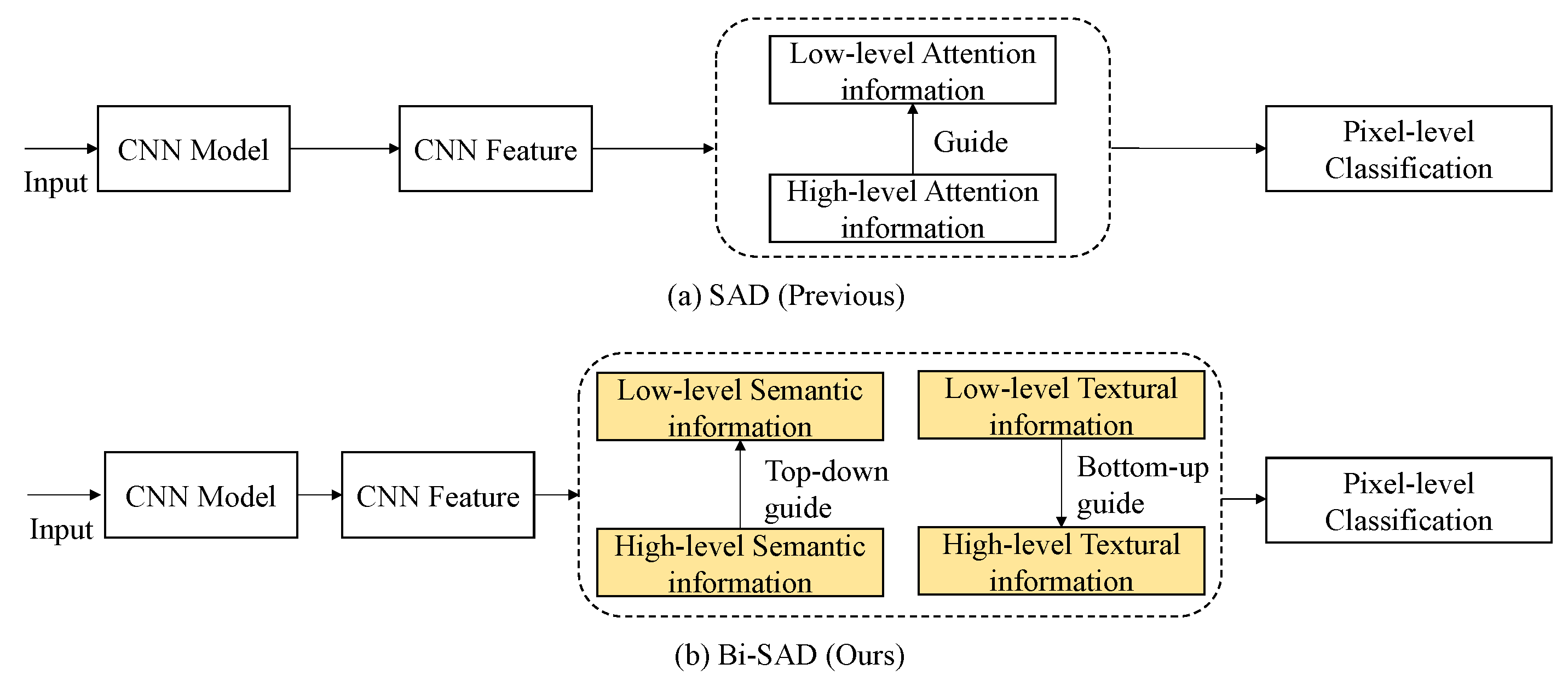
Knowledge distillation is a method to improve the performance of a compact model by transferring knowledge from the cumbersome model, where a compact model is defined as student model and a well-trained cumbersome model is defined as the teacher model [38]. In general, knowledge distillation can be divided into two categories: teacher–student (T–S) methods [38,39,40,41,42] and self-distillation methods [43,44,45,46]. For T–S methods, a compact student model learns the behavior of a cumbersome teacher model to acquire better generalization. For self-distillation methods, the network learns from itself to enhance the performance. In cloud detection task, as there are only two categories, i.e., cloud and background; T–S methods [38,39,40,41,42] tend to make the student model only distill little knowledge from inter-class similarity of teacher’s softened outputs. On the contrary, the self-distillation method [43] performs better in this case. Besides, as no teacher model is required, the training efficiency of self distillation method is higher. However, in the current self-distillation method, SAD [43], as shown in Figure 1a, the entire attention maps of lower layer mimic that of higher layer. This loses the attention information of the lower layer and degrades the representation of textural information of the clouds, causing coarse boundaries of clouds.
In this work, we propose a novel bidirectional self-attention distillation (Bi-SAD) method for compact and accurate cloud detection. It can get more reliable cloud detection results by reinforcing representation learning from itself without additional external supervision. As illustrated in Figure 1b, Bi-SAD presents a bidirectional attention maps learning, which contains two mimicking flows—forward semantic information learning and backward textural information learning. To get more reliable predictions, the semantic information of lower block mimics the semantic information of deeper block during the forward procedure. Meanwhile, to get more detailed boundaries, the textural information of deeper block learns the textural information of preceding feature block in the backward procedure. By introducing Bi-SAD, the network can strengthen its representations and acquire a significant performance gain.
Above all, the main contributions of this paper can be summarized as follows.
- We present a novel self-attention knowledge distillation framework, which is called Bi-SAD, for compact and accurate cloud detection in remote sensing imagery. Compared with other deep learning-based cloud detection methods, our method greatly reduces the parameter size and FLOPs, making it more suitable for practical applications.
- To enhance the feature learning of the cloud detection framework, we design a bidirectional distillation way, which is composed of backward boundaries distillation and forward inner distillation, to get detailed boundaries and reliable cloud detection results. Moreover, we systematically investigate the inner mechanism of Bi-SAD and analyze its complexity carefully.
- We conduct sufficient experiments on Gaofen-1 cloud detection dataset and achieve a great balance between compact model and good accuracy. Besides, the time point of introducing Bi-SAD and the optimization of parameters are carefully studied in the distillation process, which further improves the performance on cloud detection.
The reminder of this paper is organized as follows. In Section 2, we introduce the Bi-SAD framework in details. In Section 3, we describe the dataset and present experiments results to validate the effectiveness of our proposed method. In Section 4, we discuss the results of proposed method. Finally, Section 5 gives a summary of our work.
2. Materials and Methods
In this section, we describe our method in detail. The framework of Bi-SAD is presented in Section 2.1. The detailed generation of semantic attention map and textural attention map is discussed in Section 2.2. Section 2.3 presents the specific implementation process of Bi-SAD. Section 2.4 gives the complexity analysis of Bi-SAD.
2.1. Overview
The overall framework of our proposed Bi-SAD is shown in Figure 2a. It is a general distillation method and has no strict requirements on backbone. In this paper, we use ResNet-18 [35] as the backbone to illustrate our method. We denote the conv2_x, conv3_x, conv4_x, and conv5_x of ResNet [35] as block1, block2, block3, and block4, respectively.
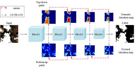
The attention map in Figure 2b,c shows where the network focuses and is based on the attention transfer operation [42]. Considering that the boundaries area of the attention map contains more textural information and the inner area contains more semantic information, we define the boundaries area of attention map as textural attention map, and the inner area of attention map as semantic attention map, respectively. We define Mask B and Mask I as the binary mask of the boundary area and the inner area of the prediction, respectively. The top row of Figure 2a represents the layer-wise top-down attention distillation, where the semantic attention map of preceding block to mimic that of a deeper block, e.g., block3 block4 and block2 block3, and the bottom row of Figure 2a represents the layer-wise bottom-up attention distillation, where the textural attention map of higher block to mimic that of a lower block, e.g., block2 block1 and block3 block2.
We get our ideas from the following facts. First, when a cloud detection network is trained properly, attention maps of different layers would capture rich and diverse information. Second, directly conducting full feature attention map mimicking would unavoidably introduce some noise from background areas where there are snow, buildings, coast lines, roads, etc. Finally, the deeper layer has more powerful semantic information, which is of vital importance to classify the clouds, and the lower layer has more detailed textural information, which is helpful to get accurately localization and detailed boundaries. Considering that it is better to mimic a region-based attention map and integrate the semantic information and textural information in the network learning, we design a bidirectional self-attention distillation.
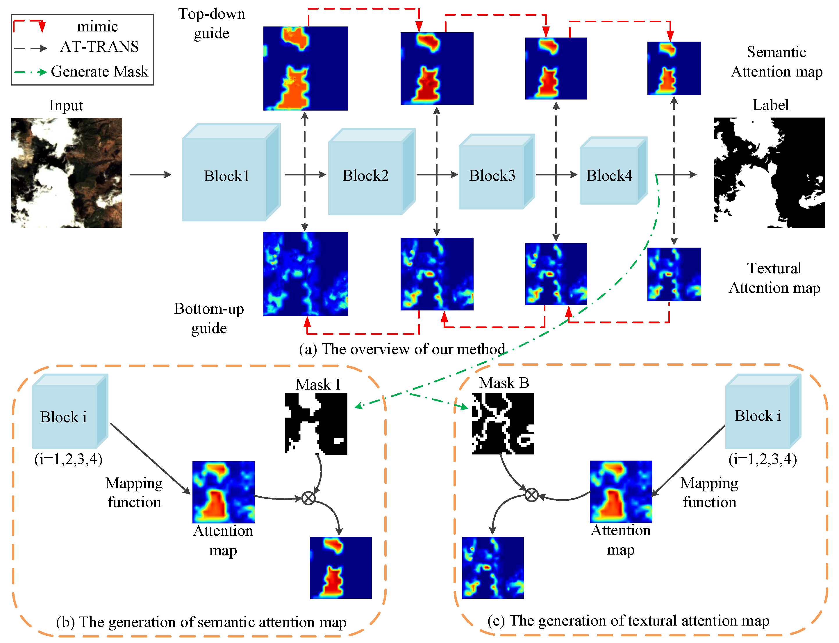
2.2. Generation of Attention Map
As depicted in Figure 2a, for the boundaries of the clouds and the inner area of the clouds, we design a backward learning flow and forward learning flow, respectively. First, we need to get the attention maps through the attention mapping function. Let us denote the activation output of the n-th layer of the network as , where , , and represent the channel, width, and height, respectively. The attention map is generated by mapping function
The absolute value of each element in attention map indicates the importance of the element on the output. As a result, we can design a mapping function via computing statistics of these values along the channel dimension. More specifically, we design a mapping function by summing the squared activations along the channel dimension. We denote
as the mapping function.
The framework of the generation of textural and semantic attention map can be seen in Algorithm 1. In the following, we demonstrate the generation of textural attention map and semantic attention map in detail.
| Algorithm 1 Generation of textural and semantic attention map. |
| Input: The feature maps of Block1, Block2, Block3, Block4, ; The prediction result R; Output: The textural attention maps ; The semantic attention maps ; 1: Step1: Generate Masks 2: Extracting the boundaries of R; 3: Get Mask by expanding the boundaries of R; 4: Get Mask ; 5: Step2: Get Textural and Semantic Attention Maps 6: for Block do 7: Downsaple Mask to match the spatial size of ; 8: Downsaple Mask to match the spatial size of ; 9: ; 10: ; 11: end for 12: return ; |
2.2.1. Textural Attention Map
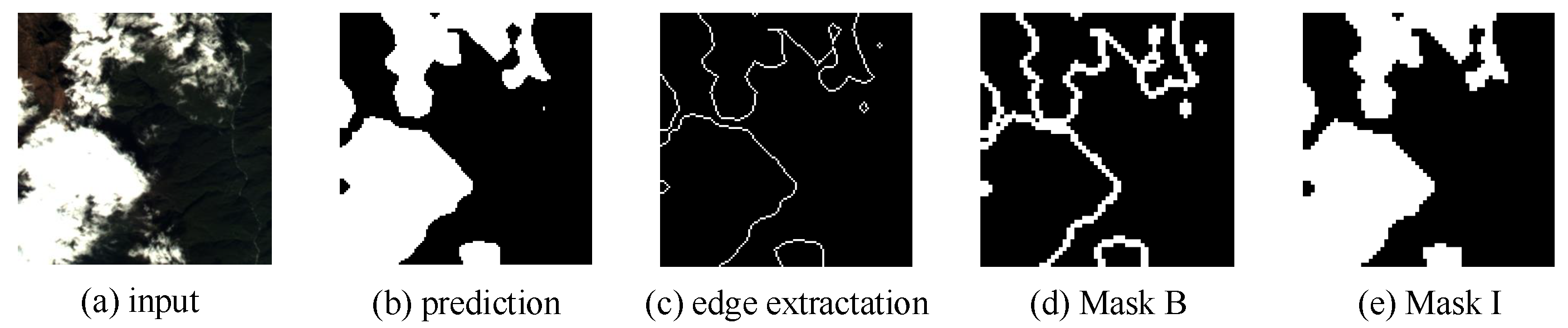
We use Mask B and the attention map to generate the textural attention map. For each individual image, as shown in Figure 3a, first, we use Laplace Operator to extract the boundaries of the prediction as shown in Figure 3c. Then, we use morphological expansion method to expand the boundaries and term it as Mask , as shown in Figure 3d.
Figure 2c shows the generation of textural attention map: for Block i, it first generates attention map by mapping function, and then generates textural attention map by using attention map to multiply the downsampled Mask (the downsampled Mask refers to downsampling Mask to match the spatial size of feature map ). We can see from Figure 2c that the textural attention map contains not only the boundaries of the big clouds, but also some small pieces of the clouds, and in these areas, the network needs refined textural information to capture detailed boundaries of clouds.
2.2.2. Semantic Attention Map
We use Mask I and the attention map to generate a semantic attention map. For each single image, as shown in Figure 3a, we use the prediction subtracting Mask to generate Mask , as shown in Figure 3e.
Figure 2b shows the generation of semantic attention map: for Block i, similar to the generation of textural attention map, it generates semantic attention map by using attention map to multiply the downsampled Mask (the downsampled Mask refers to downsampling Mask to match the spatial size of feature map ). As shown in Figure 2b, semantic attention map contains the inner area of the big clouds, and in these areas, the network needs strong semantic information to make a reliable prediction of clouds.
2.3. Bidirectional Self-Attention Knowledge Distillation
The whole training procedure can be divided into two stages, i.e., the network training itself and adding Bi-SAD to training. In the former stage, the network does not capture useful information very well, and therefore these layers that previous layer want to mimic, i.e., the distillation targets are of low quality. Therefore, the network needs to learn by itself. When the detection network is trained to a reasonable level so that the distillation targets capture useful information, we add Bi-SAD to training. Here, we assume the network half-trained to 5000 epochs.
We term the forward semantic information learning as Inner-SAD, and the backward textural information learning as Boundary-SAD. The framework of the training procedure of Bi-SAD can be seen in Algorithm 2. In the following, we discuss the training procedure of Bi-SAD in details.
In order to obtain the semantic information and textural information acquired in Inner-SAD and Boundary-SAD, we set an attention transformer after each of block1, block2, block3, and block4 of the backbone, which is termed as AT-TRANS. As shown in Figure 2a, we use the black dotted line to represent the procedure of attention transformer. There are several operations in the attention transformer: First, we use to get the 2D attention map from 3D tensor . Second, as the size of original attention maps is different from that of targets, we utilize bilinear upsampling to match the spatial dimensions. Then, we acquire area-of-interest by multiplying downsampled Mask B or downsampled Mask I. In Inner-SAD, we use the downsampled Mask (Mask represents the Mask I of Block n), denoted as to generate the semantic attention map, and in Boundary-SAD, we use the downsampled Mask (Mask represents the Mask B of Block n), denoted as , to produce the textural attention map. Finally, we use the normalization function to normalize the vector above. AT-TRANS is represented by a function:
where represents or .
| Algorithm 2 Bidirectional self-attention knowledge distillation. |
| Input: The semantic attention maps ; The textural attention maps ; Output: Forward distillation loss ; Backward distillation loss ; 1: Step1: Inner-SAD 2: Initialize ; 3: for do 4: Upsample to match the spatial size of ; 5: Normalize and ; 6: ; 7: end for 8: Step2: Boundary-SAD 9: Initialize ; 10: for do 11: Upsample to match the spatial size of ; 12: Normalize and ; 13: ; 14: end for 15: return |
2.3.1. Inner-SAD
As shown in Figure 2a, the red dotted line at the top represents the flow of forward semantic information learning. During the forward mimicking procedure, the semantic attention map of lower block mimics the semantic attention map of higher block, e.g., block3 block4 and block 2 block3. A successive top-down layer-wise distillation loss, whose direction is forward, is formulated as follows,
where is usually defined as an loss, and is the target of the top-down layer-wise distillation loss.
2.3.2. Boundary-SAD
Meanwhile, as shown in Figure 2a, the red dotted line at the bottom represents the flow of backward detailed boundaries information learning. During the backward learning procedure, the boundaries attention map of deeper block learns the boundaries attention map of preceding feature block, e.g., block2 block1 and block3 block2. A successive bottom-up layer-wise distillation loss, whose direction is backward, is formulated as follows,
where is usually defined as an loss, and is the target of the bottom-up layer-wise distillation loss. Besides, as blocks represent conv2_x, conv3_x, conv4_x, and conv5_x of ResNet [35], . We do not assign different weights to different Bi-SAD paths, although it is possible. Besides, considering that the attention maps of adjacent layers are semantically closer than those of non-neighboring layers, we perform mimicking the attention maps of the adjacent layers successively instead of any other paths (e.g., block 2 block4, block3 block1).
The overall training loss of the detection model is
where is the standard entropy loss, and and are the distillation loss weight balancing factors.
2.4. Complexity Analysis of Bi-SAD
In order to evaluate the efficiency of our Bi-SAD, we analyze its complexity for the distillation operation. The computational cost of Bi-SAD mainly includes the generation of attention maps and the learning process. The cost of the former and the latter are and , respectively,
where and , and , and , and and are , , , and of width and height of the original input image, respectively, and .
By analysis, we can get the calculation complexity of Bi-SAD:
In addition, compared with T–S methods, our Bi-SAD has a lower calculation complexity of the distillation operation, which can significantly reduce storage space and increase computing speed. Specifically, the method in [40] reaches , the method in [41] reaches , and our Bi-SAD only reaches , where C represents the number of channels in feature map; N represents the number of classes; and W and H represent the width and height dimensions of feature map, respectively.
3. Experiments
In this section, we comprehensively evaluate the proposed Bi-SAD on GaoFen-1 satellite images. Specifically, we first present description of experimental details. Then, we discuss the performance of Bi-SAD qualitatively and quantitatively. Finally, we also conduct a comparative experiment with the state-of-the-art distillation models and deep learning-based cloud detection models.
3.1. Experiments Settings
3.1.1. Dataset
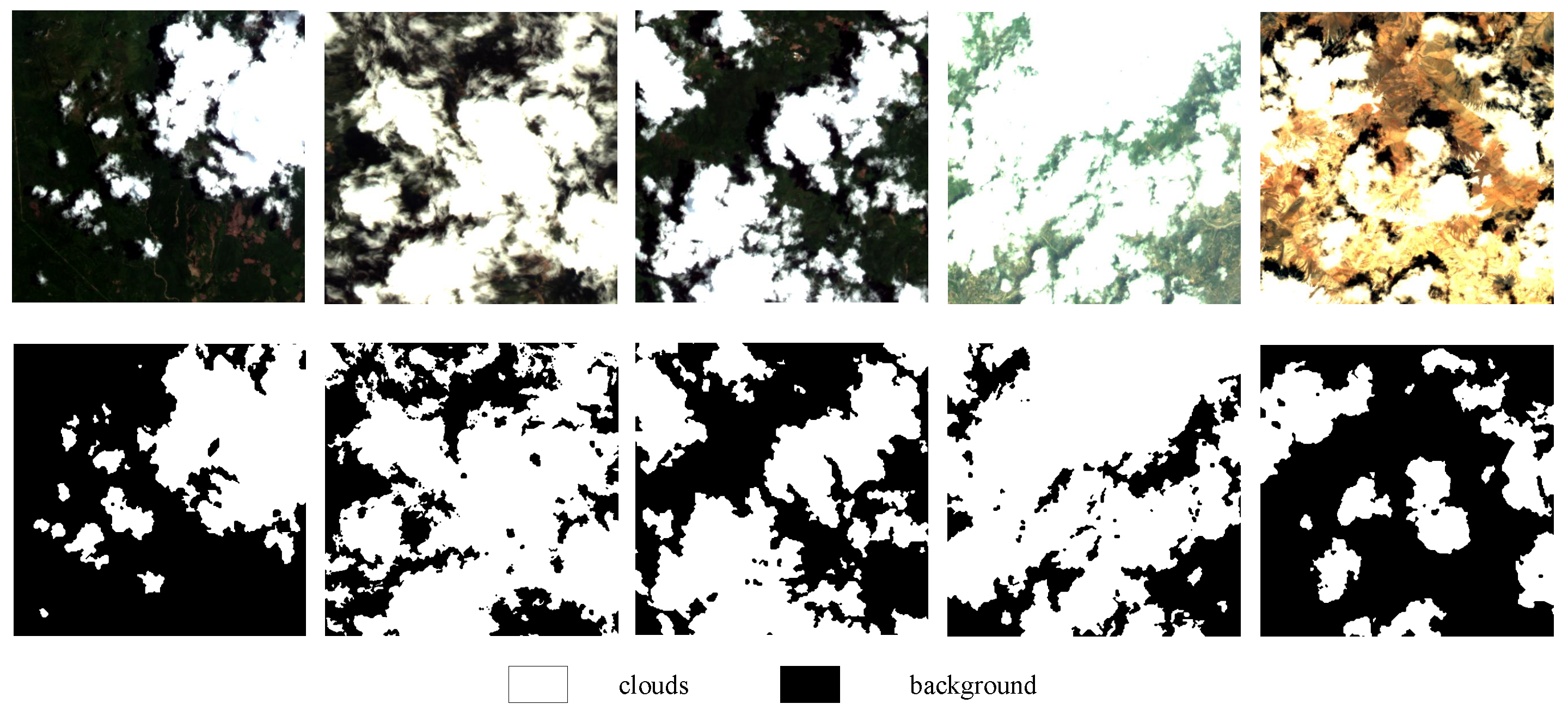
In order to quantitatively evaluate the performance of our method, we use the public accessible GaoFen-1 dataset released by Li et al. [8] in the experiments, where there are three visible bands and a near-infrared band. The images were acquired from May 2013 to August 2016 in different global regions [8]. The resolution of the image is 16 m. The whole dataset contains 108 globally distributed scenes and covers different clouds types and land cover types, including water, urban areas, forest, barren, and ice/snow. Thus, we can have a comprehensive test of our method under different conditions. There are only clouds and background in our experiments, where small clouds, broken clouds, thick clouds and thin clouds are all marked as clouds, and background, clear-sky, cloud shadow, and other non-cloud bright objects are marked as background, as shown in Figure 4. The whole 108 scenes whose sizes are 10,000 × 9000 pixels are divided into training set (87 scenes) and testing set (21 scenes), according to the proportion of 8:2. Both the training set and test set contain the clouds of different sizes, shapes, and levels of cloud coverage and background of various scenes. The training set and testing set are cropped into 41,434 slices and 10,359 slices, and the size of each slice is 513 × 513 pixels.
3.1.2. Network Design
In the experiment, we evaluate the performance enhancement of our proposed method on a popular compact model, i.e., ResNet18 [35]. More specifically, to further increase the speed and reduce the amount of parameters, we denote the vanilla ResNet18 as 1× model, and directly halve channels of each layer to obtain the 0.5× model. Then halve again to obtain the 0.25× model, and the 0.25× model has a smaller model size than the vanilla ResNet18 by 41.75 MB.
Baseline Setup. We utilize the 0.25× ResNet18 as the backbone, and we employ 32× bilinear upsampling to predict, which is a very simple FCN [47] alike semantic segmentation model. We use the simple yet general model to verify the wide universality and the great generalization of our proposed method.
3.1.3. Evaluation Metrics
We evaluate the model in terms of accuracy and efficiency.
For quantitative evaluation of the detection accuracy, we use mean intersection over union (), score, overall accuracy () [47] as the measurement. Notably, a large score suggests a better result. Besides, and that indicates overall pixel accuracy, are also calculated for a comprehensive comparison with different models. Let be the number of pixels of class i predicted to belong to class j, and k be the number of classes. We calculate , , and with the following formula,
where is the number of pixels correctly detected as cloud, is the total number of pixels detected as cloud, and is the number of cloud pixels in ground truth.
For quantitative evaluation of the model efficiency, we use execution time [48], the model size and the calculation complexity [41] to measure. The execution time is represented by the inference time of the network. We input the slice with 513 × 513 pixels resolution of the whole testing sets, and calculate the average time of each image as the inference time. The model size is expressed in terms of the number of network parameters. And the calculation complexity is represented by the sum of the floating-point operations (FLOPs) in once forward on a fixed input size.
3.2. Training and Testing Details
Our experiments are performed on one RTX-2080Ti GPU with PyToch 1.1.
During the training procedure, the input image is the slice with 513 × 513 pixels. In order to prevent overfitting, some data augmentation methods are applied, such as random scale, random horizontal, and vertical flipping. The stochastic gradient is selected as the optimizer for our experiments with a momentum of 0.9. We use a “poly” learning rate policy [20] in training with a base learning rate of 0.002 and a power of 0.9. Loss weight balancing factors and are empirically set as 0.5 and 0.5, respectively. We train our network from scratch for 30,000 iterations with a batch size of 40. For the method of without knowledge distillation approach, the total loss is cross-entropy loss between prediction and ground truth. For the methods based on T–S knowledge distillation and SAD, the total loss is cross-entropy loss [47] plus distillation loss.
During the stage of test, we keep the original resolution of image instead of resizing it to a fixed size, and all of our test results are keeping the same scale. In our experiments, we use the method of sliding window detection to implement the inference for the every whole image. In details, the size of the sliding window is the same as the input size in the training stage, i.e., 513 × 513 pixels.
3.3. Ablation Studies
In this section, we investigate the effects of Boundary-SAD and Inner-SAD. Besides, we also show the experiments of parameter optimization.
3.3.1. The Effect of Boundary-SAD
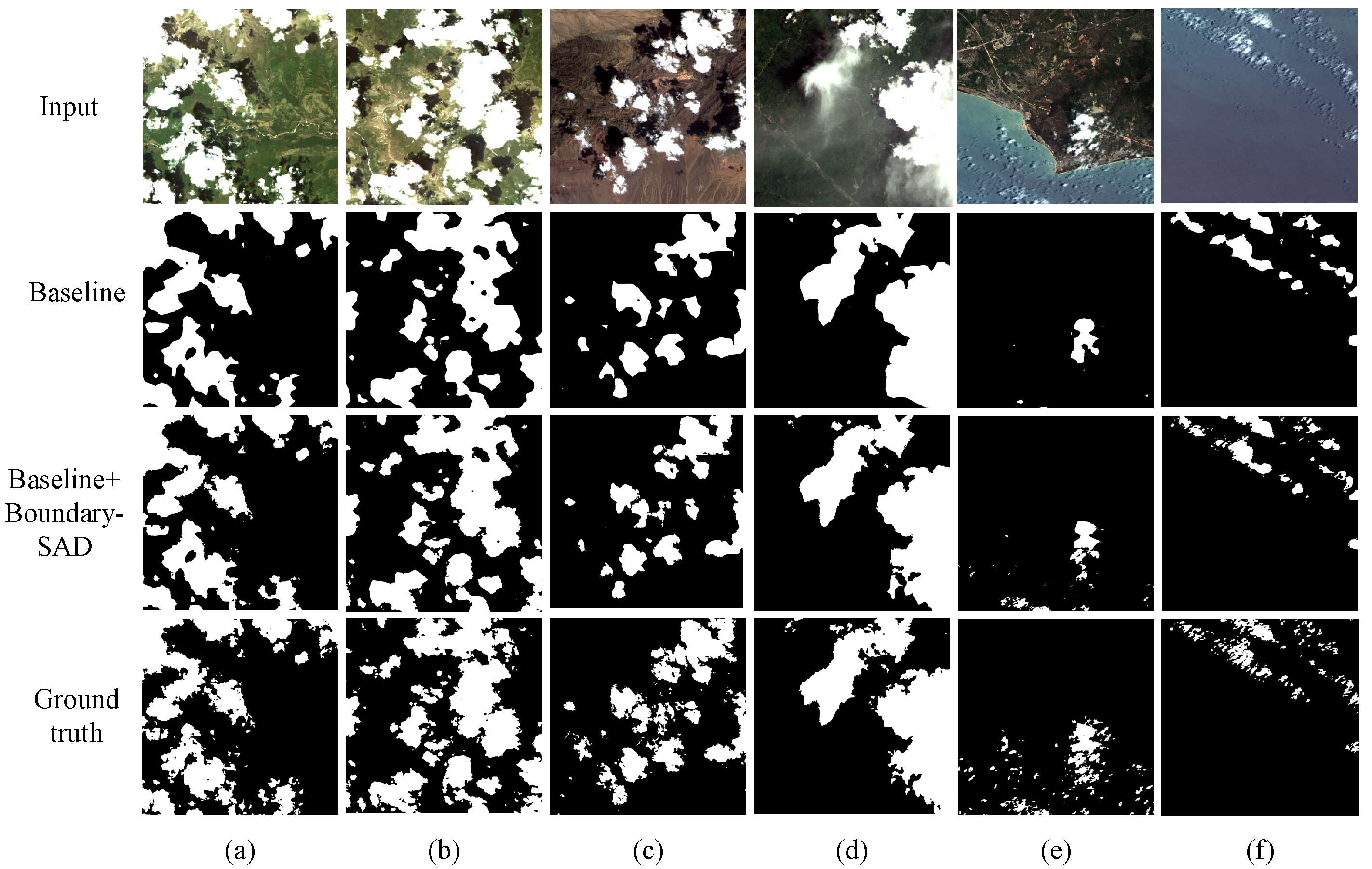
In order to capture cloud details more accurately, we add Boundary-SAD to the baseline model. Table 1 shows that there is a 1.28% enhancement in mIoU. As shown in Figure 5, after adding Boundary-SAD, the predictions of boundaries of clouds and small piece of clouds are more accurate. Boundary-SAD gives the model a better ability to capture details in clouds.
3.3.2. The Effect of Inner-SAD
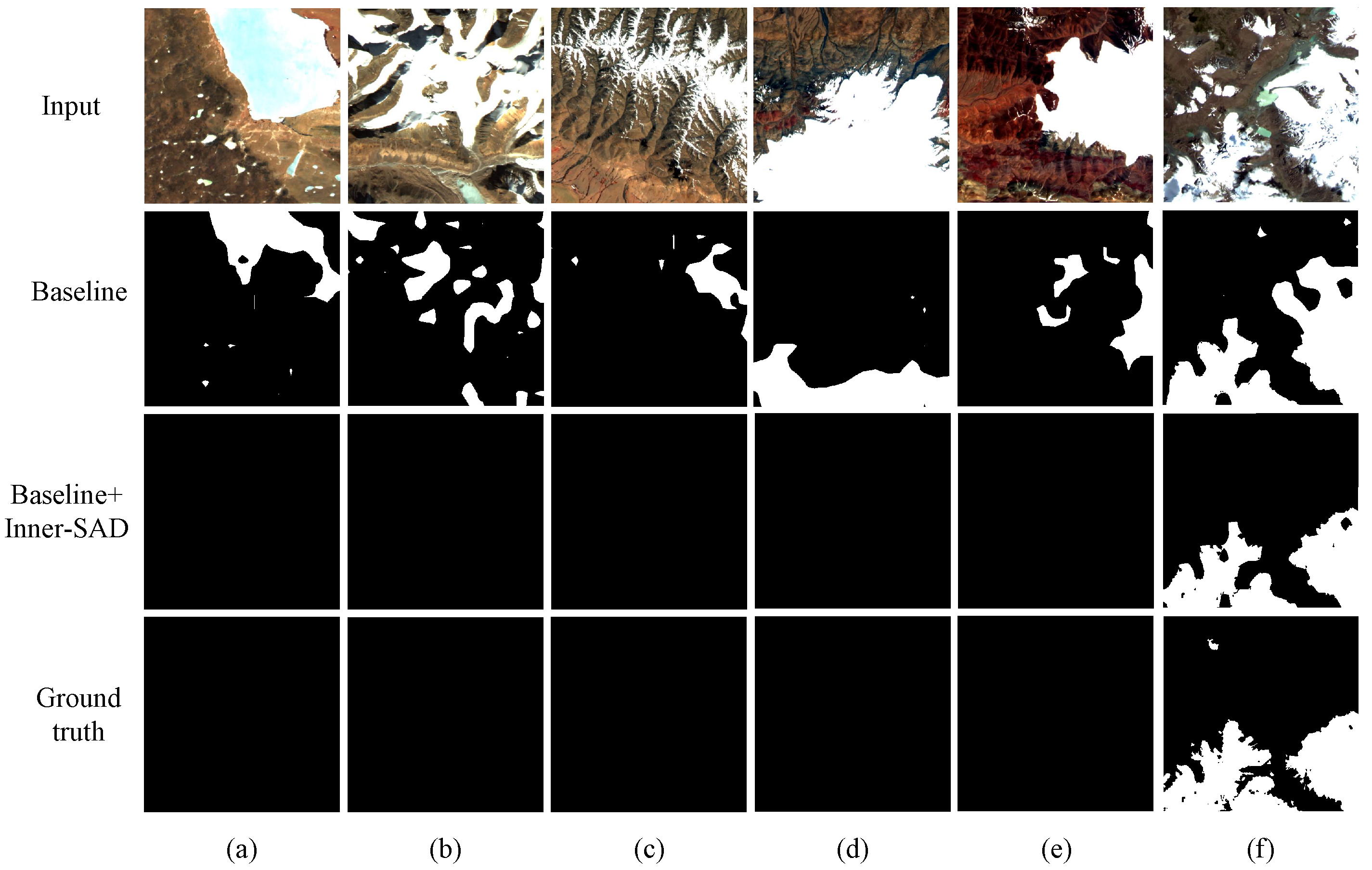
To make more reliable predictions, we add Inner-SAD to the baseline model. Table 1 shows that the improvement of mIoU is 2.01%. As shown in Figure 6, after introducing Inner-SAD to the network, the results present less misclassified pixels than baseline model. Inner-SAD gives the model a better ability to distinguish between snow/ice and clouds.
Besides, as shown in Table 1, our method achieves a high accuracy of 96.72%, with small model size, low calculation complexity, and fast inference time. When Bi-SAD is added to baseline, the network performance has been further improved, i.e., a 2.63% gain in mIoU, without increasing the amount of parameters, computational complexity and inference time. It proves that our method of combining forward semantic information learning and backward textural information learning is effective.
3.3.3. The Effect of Mimicking Direction
To investigate the effect of mimicking direction on performance, we reverse the direction: for the boundaries region of the cloud, the lower layers mimic higher layers, and for the inner region of the cloud, the higher layers mimic lower layers. It decreases the performance of the baseline model from 84.40% to 83.52%. This is because low-level attention maps contain more textural information, i.e., details and high-level attention maps contain more high-level semantic information. Reversing the mimicking direction will inevitably hamper the learning of the crucial clues for the cloud detection.
3.3.4. Parameter Optimization
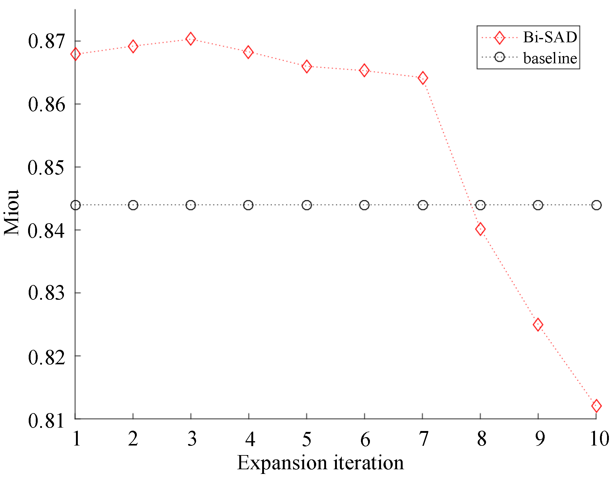
During the generation of the masks, we use Laplace Operator to extract the boundaries, and use morphological expansion method to expand the boundaries to acquire the Mask B (Section 2.2), where there is a hyperparameter, i.e., the expansion iteration. Besides, we assume a half-trained model before we introduce Bi-SAD to the training. In this study, we did the experiments to find the fitting hyperparameter.
The hyperparameter of the masks. Figure 7 shows the resulting mIoU of the varying expansion iteration, and we can see that when the iteration is larger than 7 (iteration > 7), the performance of the Bi-SAD is lower than baseline. This is because as the expansion iteration grows, the boundaries of clouds will grow in Mask B and the center region of clouds will decrease in Mask I, which may cause Mask B contains more center region of clouds. If the boundaries and inner area represented by Mask B and Mask I are not accurate, the textural information and semantic information will not be learned very well. As a result, when the iteration is larger than 7, the performance will drop a lot. As shown in Figure 7, the results show that the value of 3 turns out to be optimal, and in the experiment, we use 3 as the expansion iteration to generate Mask B.
The time point to add Bi-SAD. Here, we research the time points to add Bi-SAD. As shown in Table 2, we can see that different time points of adding Bi-SAD almost converge to the same point, and 5000 is relatively better. We think that this it caused by the quality of the distillation targets produced by later layers and the optimization speed. In the earlier training stage, as the distillation targets produced by later layers are of low quality, this may introduce some noise to training. In the later training stage, the quality of the distillation targets is well, but as the learning rate drops, the optimization speed is slow. Besides, we find that after introducing Bi-SAD to network, the network has a more rapid speed of convergence. In the experiments, we add Bi-SAD to training when the network trained to 5000.
3.4. Comparison with The State-of-the-Art Distillation Methods
In this section, we make a comparison between our Bi-SAD with state-of-the-art self distillation method and T–S distillation methods.
For T–S distillation methods, we denote the 1.0× ResNet18 with 32× upsamping as the teacher model and denote the baseline model as the student model. Two state-of-the-art T-S distillation methods are selected in this experiment, named zero+first [40] and pixel+pair [41]. For self distillation method, we make a comparison between our Bi-SAD and SAD [43].
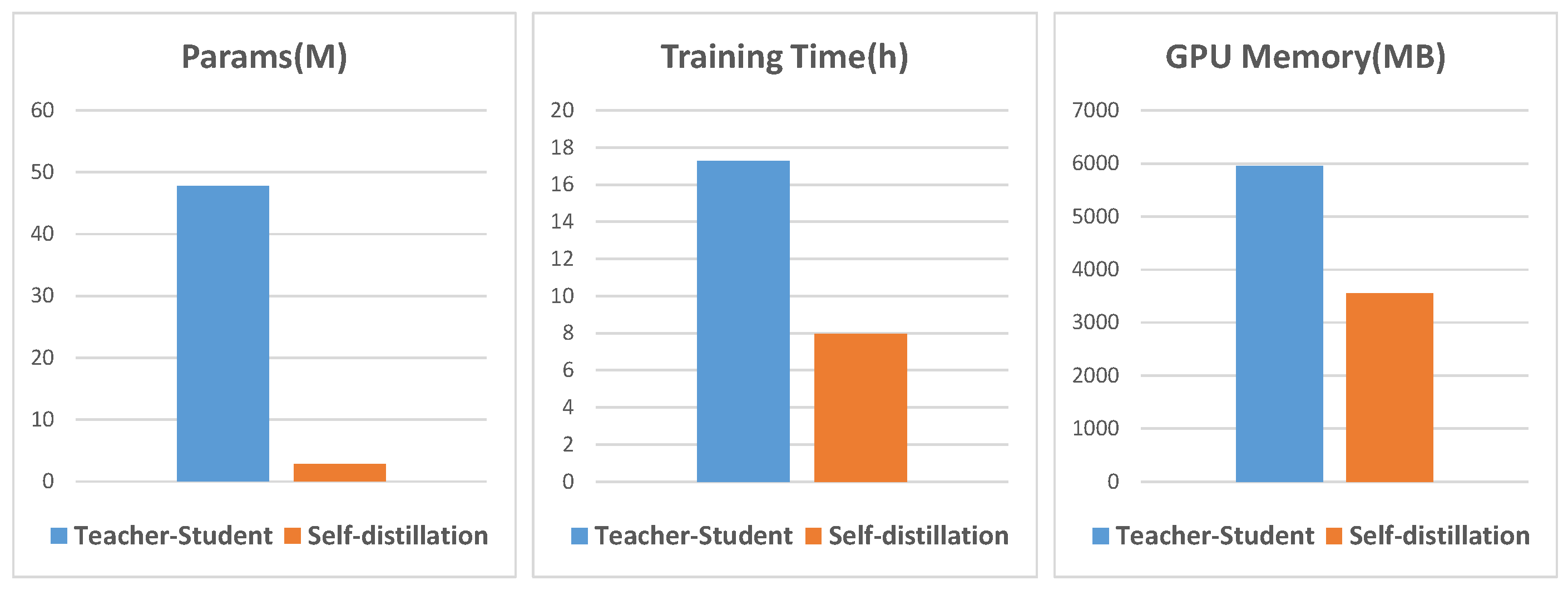
The results are shown in the Table 3. We find that after training with our Bi-SAD, the student model almost reaches the same performance as the teacher model and even better on mIoU and , and our Bi-SAD also outperforms the state-of-the-art distillation methods, which proves that our Bi-SAD is more powerful in cloud detection. Besides, as shown in Figure 8, as the teacher model is required to be trained well in advance in T–S methods, comparing with T–S methods in terms of the training time, the amount of parameters, and GPU memory usage, our Bi-SAD is more efficient in the training phase.
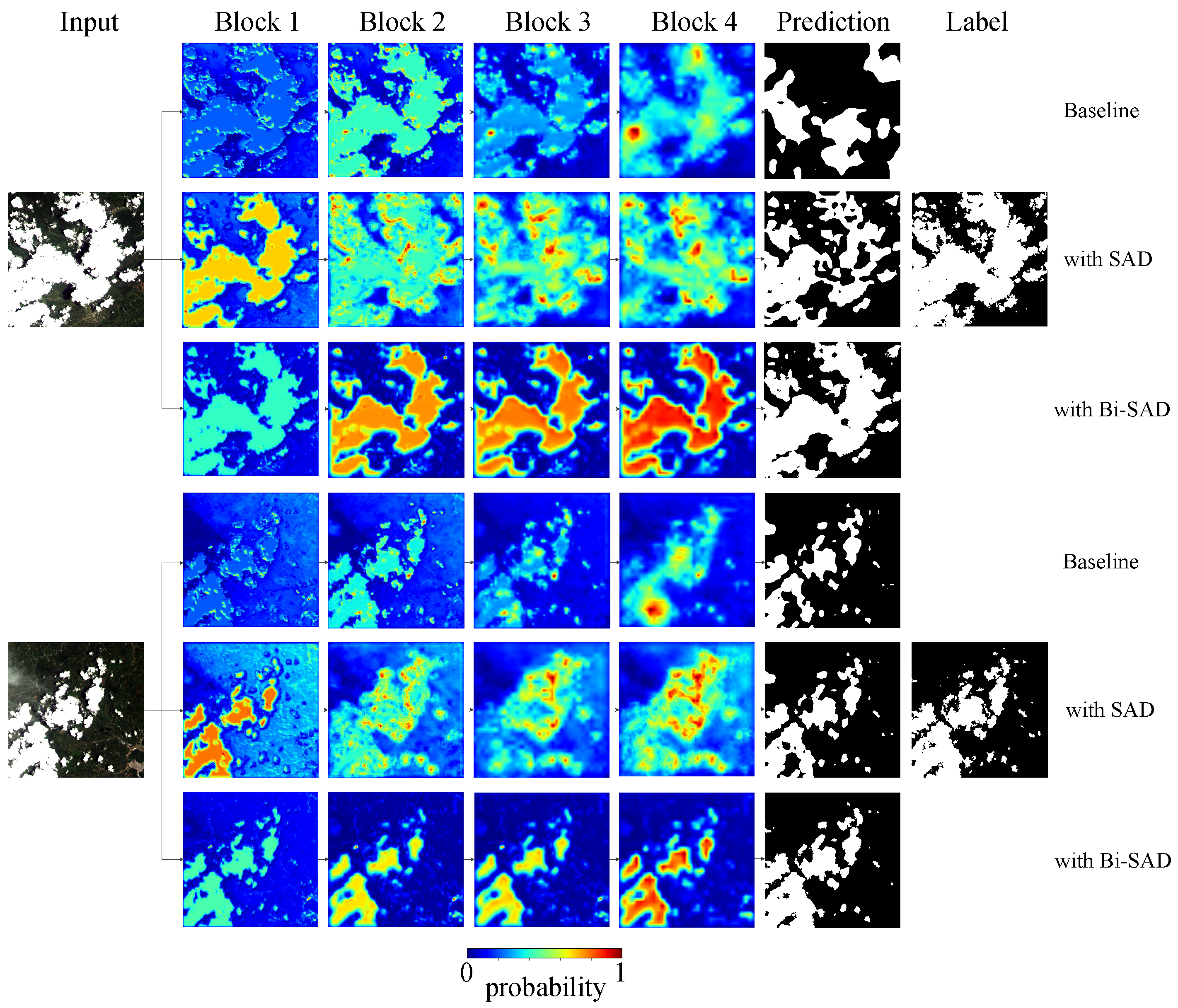
Further, as shown in Figure 9, we can see that (1) with the forward mimicking and the backward mimicking in Bi-SAD, the high-level attention map not only contains rich semantic information, but also incorporates textural information, which is vital to make a precise prediction. (2) After adding self-attention distillation, attention maps of the network become more explainable. Because the shape of attention maps are getting closer to the shape of the cloud, this also shows that the network focuses on the clouds, so the performance is better. And this phenomenon is more obvious in Bi-SAD than SAD.
3.5. Comparison with The State-of-the-Art Deep Learning-Based Cloud Detection Approaches
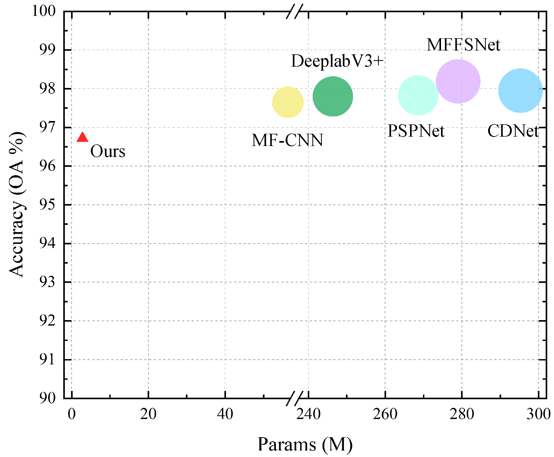
To comprehensively evaluate the proposed method from the model parameter amount, speed, and accuracy, we make a comparison with the state-of-the-art deep learning-based cloud detection models including MFFSNet [24], CDNet [27], PSPNet [23], DeeplabV3+ [22], and MF-CNN [25], as shown in Table 4. Figure 10 quantitatively shows the accuracy, parameters, and FLOPs of these methods; we can see that although there exists as small difference in performance, our method has fewer parameters, lower calculation complexity, and faster inference speed. Specifically, by comparing our method with the current highest precision MFFSNet, the parameter size and FLOPs are reduced by 100 times and 400 times, respectively, with a small drop in accuracy, and the speed is increased by ~7 times. It also shows that our method is more conducive to practical application.
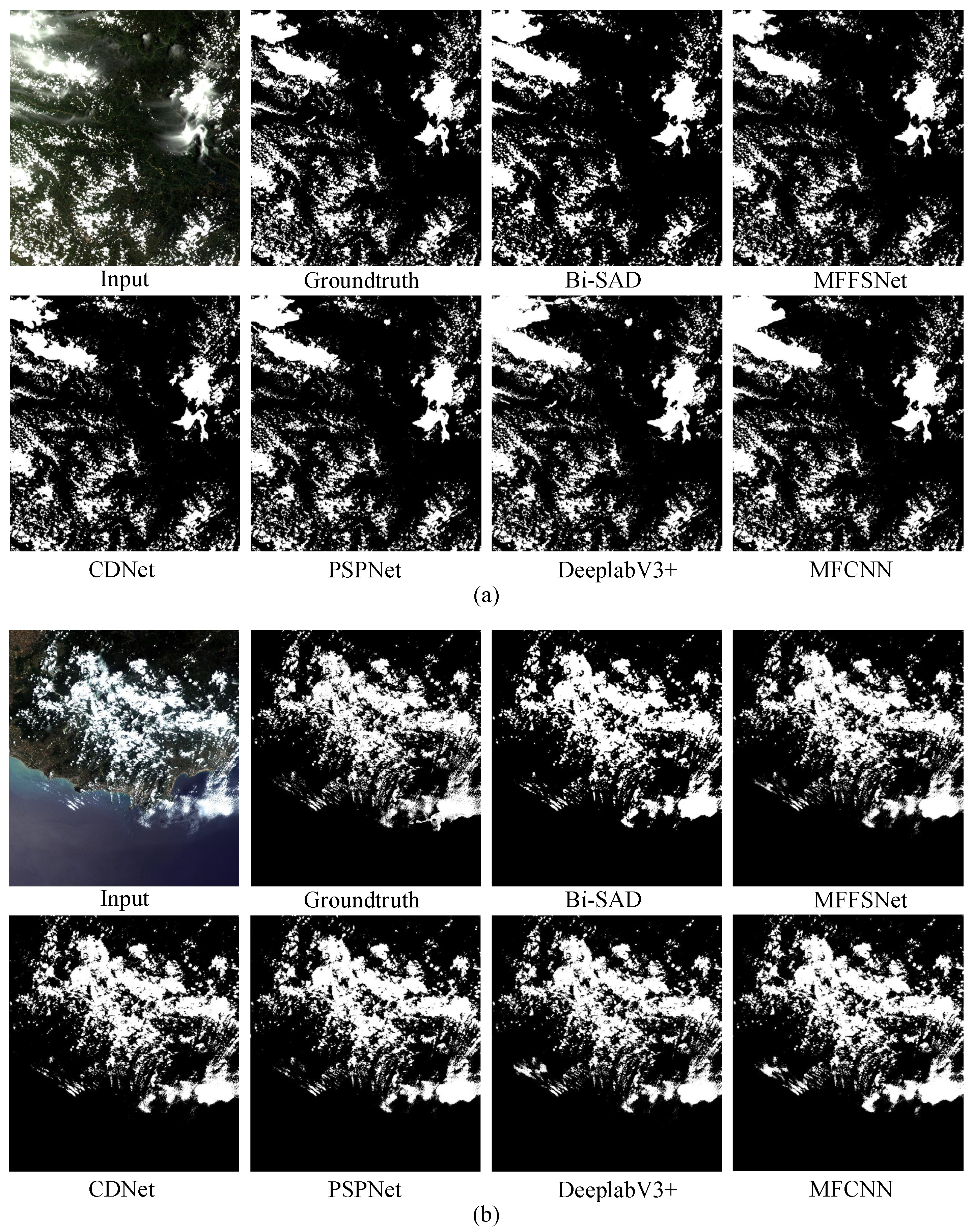
Besides, Figure 11 qualitatively shows that our method performs well in the scene of forest, roads, water, and coastline, and can accurately capture thin clouds, small piece of clouds, and boundaries of clouds. Moreover, as shown in Figure 11, we can see that in big clouds, thin clouds, small pieces of clouds, and broken clouds our network has a competitive performance with the state-of-the-art cloud detection models.
4. Discussion
The experimental results in Section 3.3 and Section 3.4 prove that the proposed method can effectively improve the performance of cloud detection network, our method has a performance enhancement over other distillation methods and the training efficiency of our method is higher. There are several reasons: First, through our proposed two mimicking flows—forward semantic information learning and backward detailed textural information learning—the model indeed enhances its representation of clouds, so the performance is improved. Second, in terms of cloud detection, compared with existing T–S distillation methods, the self-distillation method can more effectively capture useful information through self-attention mechanism. Third, as the distillation information of our proposed method comes from different layers of the network, no teacher model is required, so the training efficiency of our proposed method is higher.
Although our method achieves a good balance between accuracy and speed, the accuracy of the model needs to be further improved. We think the reason may be that the limited parameter amount limits the feature learning ability of the model to some extent.
We will investigate how to design a network structure with a small amount of parameters and low computational complexity, but with strong feature extraction capabilities to further improve the performance and speed in our future work.
5. Conclusions
In this work, we propose a novel bidirectional self-attention distillation method for compact and accurate cloud detection. Our method takes full use of the information of low-level and high-level attention map to improve the representation learning of DCNN-based cloud detection models. Experiments based on the GaoFen-1 cloud dataset demonstrate that our method outperforms other state-of-the-art distillation methods and achieves a great trade-off between accuracy and speed. Extensive experiments and analysis demonstrate the effectiveness of our approach. In future work, we will pay more attention to further improving the accuracy of the cloud detection model with limited parameters.
Author Contributions
Formal analysis, Y.C.; Funding acquisition, K.F., X.S., W.D., Z.Y., and L.W.; Investigation, Y.C.; Methodology, Y.C.; Supervision, K.F., X.S., W.D., Z.Y., and L.W.; Visualization, Y.C.; Writing—original draft, Y.C.; Writing—review and editing, Y.C., K.F., X.S., W.D., Z.Y., Y.F., and L.W. All authors have read and agreed to the published version of the manuscript.
Funding
This work is supported by the National Natural Science Foundation of China under Grants 41701508 and 61725105.
Acknowledgments
The authors would like to thank all their colleagues in the lab, who generously provided their original images and helped to annotate the images. The authors are very grateful to the anonymous reviewers for their helpful suggestions.
Conflicts of Interest
The authors declare no conflict of interest.
References
- Fu, K.; Chang, Z.; Zhang, Y.; Xu, G.; Zhang, K.; Sun, X. Rotation-aware and multi-scale convolutional neural network for object detection in remote sensing images. ISPRS J. Photogramm. Remote Sens. 2020, 161, 294–308. [Google Scholar] [CrossRef]
- Wang, P.; Sun, X.; Diao, W.; Fu, K. FMSSD: Feature-Merged Single-Shot Detection for Multiscale Objects in Large-Scale Remote Sensing Imagery. IEEE Trans. Geosci. Remote Sens. 2019, 58, 3377–3390. [Google Scholar] [CrossRef]
- Zhang, Y.; Rossow, W.B.; Lacis, A.A.; Oinas, V.; Mishchenko, M.I. Calculation of radiative fluxes from the surface to top of atmosphere based on ISCCP and other global data sets: Refinements of the radiative transfer model and the input data. J. Geophys. Res. Atmos. 2004, 109. [Google Scholar] [CrossRef] [Green Version]
- Shin, D.; Pollard, J.; Muller, J.P. Cloud detection from thermal infrared images using a segmentation technique. Int. J. Remote Sens. 1996, 17, 2845–2856. [Google Scholar] [CrossRef]
- Gesell, G. An algorithm for snow and ice detection using AVHRR data An extension to the APOLLO software package. Int. J. Remote Sens. 1989, 10, 897–905. [Google Scholar] [CrossRef]
- Jedlovec, G.J.; Haines, S.L.; LaFontaine, F.J. Spatial and temporal varying thresholds for cloud detection in GOES imagery. IEEE Trans. Geosci. Remote Sens. 2008, 46, 1705–1717. [Google Scholar] [CrossRef]
- Zhu, Z.; Woodcock, C.E. Object-based cloud and cloud shadow detection in Landsat imagery. Remote Sens. Environ. 2012, 118, 83–94. [Google Scholar] [CrossRef]
- Li, Z.; Shen, H.; Li, H.; Xia, G.; Gamba, P.; Zhang, L. Multi-feature combined cloud and cloud shadow detection in GaoFen-1 wide field of view imagery. Remote Sens. Environ. 2017, 191, 342–358. [Google Scholar] [CrossRef] [Green Version]
- Irish, R.R. Landsat 7 automatic cloud cover assessment. In Algorithms for Multispectral, Hyperspectral, and Ultraspectral Imagery VI; International Society for Optics and Photonics: Bellingham, WA, USA, 2000; Volume 4049, pp. 348–355. [Google Scholar]
- Fisher, A. Cloud and cloud-shadow detection in SPOT5 HRG imagery with automated morphological feature extraction. Remote Sens. 2014, 6, 776–800. [Google Scholar] [CrossRef] [Green Version]
- Christodoulou, C.I.; Michaelides, S.C.; Pattichis, C.S. Multifeature texture analysis for the classification of clouds in satellite imagery. IEEE Trans. Geosci. Remote Sens. 2003, 41, 2662–2668. [Google Scholar] [CrossRef]
- Vivone, G.; Addesso, P.; Conte, R.; Longo, M.; Restaino, R. A class of cloud detection algorithms based on a MAP-MRF approach in space and time. IEEE Trans. Geosci. Remote Sens. 2013, 52, 5100–5115. [Google Scholar] [CrossRef]
- Xu, L.; Wong, A.; Clausi, D.A. A Novel Bayesian Spatial–Temporal Random Field Model Applied to Cloud Detection From Remotely Sensed Imagery. IEEE Trans. Geosci. Remote Sens. 2017, 55, 4913–4924. [Google Scholar] [CrossRef]
- Barnes, B.B.; Hu, C. A hybrid cloud detection algorithm to improve MODIS sea surface temperature data quality and coverage over the Eastern Gulf of Mexico. IEEE Trans. Geosci. Remote Sens. 2012, 51, 3273–3285. [Google Scholar] [CrossRef]
- Li, P.; Dong, L.; Xiao, H.; Xu, M. A cloud image detection method based on SVM vector machine. Neurocomputing 2015, 169, 34–42. [Google Scholar] [CrossRef]
- Hughes, M.J.; Hayes, D.J. Automated detection of cloud and cloud shadow in single-date Landsat imagery using neural networks and spatial post-processing. Remote Sens. 2014, 6, 4907–4926. [Google Scholar] [CrossRef] [Green Version]
- Bai, T.; Li, D.; Sun, K.; Chen, Y.; Li, W. Cloud detection for high-resolution satellite imagery using machine learning and multi-feature fusion. Remote Sens. 2016, 8, 715. [Google Scholar] [CrossRef] [Green Version]
- Tan, K.; Zhang, Y.; Tong, X. Cloud extraction from chinese high resolution satellite imagery by probabilistic latent semantic analysis and object-based machine learning. Remote Sens. 2016, 8, 963. [Google Scholar] [CrossRef] [Green Version]
- Chen, L.C.; Papandreou, G.; Kokkinos, I.; Murphy, K.; Yuille, A.L. Semantic image segmentation with deep convolutional nets and fully connected crfs. arXiv 2014, arXiv:1412.7062. [Google Scholar]
- Chen, L.C.; Papandreou, G.; Kokkinos, I.; Murphy, K.; Yuille, A.L. Deeplab: Semantic image segmentation with deep convolutional nets, atrous convolution, and fully connected crfs. IEEE Trans. Pattern Anal. Mach. Intell. 2017, 40, 834–848. [Google Scholar] [CrossRef]
- Chen, L.C.; Papandreou, G.; Schroff, F.; Adam, H. Rethinking atrous convolution for semantic image segmentation. arXiv 2017, arXiv:1706.05587. [Google Scholar]
- Chen, L.C.; Zhu, Y.; Papandreou, G.; Schroff, F.; Adam, H. Encoder-decoder with atrous separable convolution for semantic image segmentation. In Proceedings of the European Conference on Computer Vision (ECCV), Munich, Germany, 8–14 September 2018; pp. 801–818. [Google Scholar]
- Zhao, H.; Shi, J.; Qi, X.; Wang, X.; Jia, J. Pyramid scene parsing network. In Proceedings of the IEEE Conference on Computer Vision and Pattern Recognition, Honolulu, HI, USA, 21–26 July 2017; pp. 2881–2890. [Google Scholar]
- Yan, Z.; Yan, M.; Sun, H.; Fu, K.; Hong, J.; Sun, J.; Zhang, Y.; Sun, X. Cloud and cloud shadow detection using multilevel feature fused segmentation network. IEEE Geosci. Remote Sens. Lett. 2018, 15, 1600–1604. [Google Scholar] [CrossRef]
- Shao, Z.; Pan, Y.; Diao, C.; Cai, J. Cloud Detection in Remote Sensing Images Based on Multiscale Features-Convolutional Neural Network. IEEE Trans. Geosci. Remote Sens. 2019, 57, 4062–4076. [Google Scholar] [CrossRef]
- Xie, F.; Shi, M.; Shi, Z.; Yin, J.; Zhao, D. Multilevel cloud detection in remote sensing images based on deep learning. IEEE J. Sel. Top. Appl. Earth Obs. Remote Sens. 2017, 10, 3631–3640. [Google Scholar] [CrossRef]
- Yang, J.; Guo, J.; Yue, H.; Liu, Z.; Hu, H.; Li, K. CDnet: CNN-Based Cloud Detection for Remote Sensing Imagery. IEEE Trans. Geosci. Remote Sens. 2019, 57, 6195–6211. [Google Scholar] [CrossRef]
- Chai, D.; Newsam, S.; Zhang, H.K.; Qiu, Y.; Huang, J. Cloud and cloud shadow detection in Landsat imagery based on deep convolutional neural networks. Remote Sens. Environ. 2019, 225, 307–316. [Google Scholar] [CrossRef]
- Shao, Z.; Deng, J.; Wang, L.; Fan, Y.; Sumari, N.S.; Cheng, Q. Fuzzy autoencode based cloud detection for remote sensing imagery. Remote Sens. 2017, 9, 311. [Google Scholar] [CrossRef] [Green Version]
- Jiang, H.; Lu, N. Multi-scale residual convolutional neural network for haze removal of remote sensing images. Remote Sens. 2018, 10, 945. [Google Scholar] [CrossRef] [Green Version]
- Zhou, K.; Ming, D.; Lv, X.; Fang, J.; Wang, M. CNN-Based Land Cover Classification Combining Stratified Segmentation and Fusion of Point Cloud and Very High-Spatial Resolution Remote Sensing Image Data. Remote Sens. 2019, 11, 2065. [Google Scholar] [CrossRef] [Green Version]
- Francis, A.; Sidiropoulos, P.; Muller, J.P. CloudFCN: Accurate and robust cloud detection for satellite imagery with deep learning. Remote Sens. 2019, 11, 2312. [Google Scholar] [CrossRef] [Green Version]
- Segal-Rozenhaimer, M.; Li, A.; Das, K.; Chirayath, V. Cloud detection algorithm for multi-modal satellite imagery using convolutional neural-networks (CNN). Remote Sens. Environ. 2020, 237, 111446. [Google Scholar] [CrossRef]
- Ghorbanzadeh, O.; Blaschke, T. Optimizing Sample Patches Selection of CNN to Improve the mIOU on Landslide Detection. In Proceedings of the International Conference on Geographical Information Systems Theory, Applications and Management, Heraklion, Crete, Greece, 3–5 May 2019; pp. 33–40. [Google Scholar]
- He, K.; Zhang, X.; Ren, S.; Sun, J. Deep residual learning for image recognition. In Proceedings of the IEEE Conference on Computer Vision and Pattern Recognition, Las Vegas, NV, USA, 27–30 June 2016; pp. 770–778. [Google Scholar]
- Paszke, A.; Chaurasia, A.; Kim, S.; Culurciello, E. Enet: A deep neural network architecture for real-time semantic segmentation. arXiv 2016, arXiv:1606.02147. [Google Scholar]
- Howard, A.G.; Zhu, M.; Chen, B.; Kalenichenko, D.; Wang, W.; Weyand, T.; Andreetto, M.; Adam, H. MobileNets: Efficient Convolutional Neural Networks for Mobile Vision Applications. arXiv 2017, arXiv:1704.04861. [Google Scholar]
- Hinton, G.; Vinyals, O.; Dean, J. Distilling the knowledge in a neural network. arXiv 2015, arXiv:1503.02531. [Google Scholar]
- Romero, A.; Ballas, N.; Kahou, S.E.; Chassang, A.; Gatta, C.; Bengio, Y. Fitnets: Hints for thin deep nets. arXiv 2014, arXiv:1412.6550. [Google Scholar]
- Xie, J.; Shuai, B.; Hu, J.F.; Lin, J.; Zheng, W.S. Improving fast segmentation with teacher-student learning. arXiv 2018, arXiv:1810.08476. [Google Scholar]
- Liu, Y.; Chen, K.; Liu, C.; Qin, Z.; Luo, Z.; Wang, J. Structured Knowledge Distillation for Semantic Segmentation. In Proceedings of the IEEE Conference on Computer Vision and Pattern Recognition, Long Beach, CA, USA, 16–20 June 2019; pp. 2604–2613. [Google Scholar]
- Zagoruyko, S.; Komodakis, N. Paying more attention to attention: Improving the performance of convolutional neural networks via attention transfer. arXiv 2016, arXiv:1612.03928. [Google Scholar]
- Hou, Y.; Ma, Z.; Liu, C.; Loy, C.C. Learning lightweight lane detection cnns by self attention distillation. In Proceedings of the IEEE International Conference on Computer Vision, Jeju Island, Korea, 15–18 June 2019; pp. 1013–1021. [Google Scholar]
- Furlanello, T.; Lipton, Z.C.; Tschannen, M.; Itti, L.; Anandkumar, A. Born again neural networks. arXiv 2018, arXiv:1805.04770. [Google Scholar]
- Yim, J.; Joo, D.; Bae, J.; Kim, J. A gift from knowledge distillation: Fast optimization, network minimization and transfer learning. In Proceedings of the IEEE Conference on Computer Vision and Pattern Recognition, Honolulu, HI, USA, 21–26 July 2017; pp. 4133–4141. [Google Scholar]
- Bagherinezhad, H.; Horton, M.; Rastegari, M.; Farhadi, A. Label refinery: Improving imagenet classification through label progression. arXiv 2018, arXiv:1805.02641. [Google Scholar]
- Long, J.; Shelhamer, E.; Darrell, T. Fully convolutional networks for semantic segmentation. In Proceedings of the IEEE Conference on Computer Vision and Pattern Recognition, Boston, MA, USA, 7–12 June 2015; pp. 3431–3440. [Google Scholar]
- Garcia-Garcia, A.; Orts-Escolano, S.; Oprea, S.; Villena-Martinez, V.; Garcia-Rodriguez, J. A review on deep learning techniques applied to semantic segmentation. arXiv 2017, arXiv:1704.06857. [Google Scholar]
Figure 1.
The illustration of the detection pipeline. (a) Self-Attention Distillation (SAD) is a self-attention distillation method. It introduces a layer-wise attention distillation within the network itself to improve the performance the model. (b) Bidirectional Self-Attention Distillation (Bi-SAD) is our bi-directional attention distillation method. It uses the bottom-up textural information distillation to get more detailed cloud boundaries and the top-down semantic information distillation to get more reliable predictions.

Figure 2.
The pipeline of our proposed approach. (a) The overview of our Bi-SAD. (b,c) The details of the generation of semantic attention map and textural attention map. In panel (a), the black dotted line represents the generation of semantic attention map and textural attention map, the red dotted line represents the mimicking direction of Bi-SAD, and the green dotted line represents the generation of Mask B and Mask I.

Figure 3.
The generation of Masks. (a) Input image. (b) Prediction result. (c) Edge of the prediction result. (d) Boundaries area of attention map. (e) Inner area of attention map.
Figure 3.
The generation of Masks. (a) Input image. (b) Prediction result. (c) Edge of the prediction result. (d) Boundaries area of attention map. (e) Inner area of attention map.

Figure 4.
Example annotations of slices in GaoFen-1 dataset.

Figure 5.
Visual comparison of the results for details in clouds. Training with Boundary-SAD, the network can capture details more accurately. (a–c) Mix of small cloud and big cloud. (d) Mix of big cloud and thin cloud. (e,f) Small piece of clouds.
Figure 5.
Visual comparison of the results for details in clouds. Training with Boundary-SAD, the network can capture details more accurately. (a–c) Mix of small cloud and big cloud. (d) Mix of big cloud and thin cloud. (e,f) Small piece of clouds.

Figure 6.
Visual comparison of the results for tough cases with snow/ice. Training with Inner-SAD, the network can better separate cloud from non-cloud bright objects, such as snow and ice. (a) Wide range of ice. (b,c) Snow. (d,e) Wide range of snow. (f) Mix of ice, snow, and clouds.
Figure 6.
Visual comparison of the results for tough cases with snow/ice. Training with Inner-SAD, the network can better separate cloud from non-cloud bright objects, such as snow and ice. (a) Wide range of ice. (b,c) Snow. (d,e) Wide range of snow. (f) Mix of ice, snow, and clouds.

Figure 7.
The resulting mIoU of the varying expansion iteration. The expansion iteration is the hyperparameter in Mask B and Mask I.
Figure 7.
The resulting mIoU of the varying expansion iteration. The expansion iteration is the hyperparameter in Mask B and Mask I.

Figure 8.
Comparison of self-distillation method (our Bi-SAD) and Teacher–Student distillation method [41] in terms of parameters (measured by M), training time (measured by h), and GPU memory (measured by MB). It can be seen that SAD [43] requires 17× less parameters, 2× less training time, and reduces GPU memory usage by 40%.

Figure 9.
Predictions and attention maps of baseline model with and without self-attention distillation. When Bi-SAD is added to baseline model, the shape of attention maps and clouds are more similar, and the predictions are more precise.
Figure 9.
Predictions and attention maps of baseline model with and without self-attention distillation. When Bi-SAD is added to baseline model, the shape of attention maps and clouds are more similar, and the predictions are more precise.

Figure 10.
The accuracy, parameters, and floating-point operations (FLOPs) of different deep convolutional neural networks (DCNNs) on the GaoFen-1 cloud detection dataset, including our method, MFFSNet [24], CDNet [27], PSPNet [23], DeeplabV3+ [22], and MFCNN [25]. The FLOPs are represented by the size of corresponding labels (circle or triangle in the picture), which means the bigger the label, the larger the FLOPs. Compared with with the state-of-the-art deep learning based cloud detection models, our method uses fewer parameters and FLOPs to achieve comparable performance.

Figure 11.
Visual comparisons of cloud detection results of GaoFen-1 image with our method, MFFSNet [24], CDNet [27], PSPNet [23], DeeplabV3+ [22], and MFCNN [25]. (a) Spliced visual cloud detection results of GF-1 image(GF1_WFV2_E105.8_ N24.3_ 20140723_L2A0000305784). (b) Spliced visual cloud detection results of GaoFen-1 image(GF1_WFV4_E109.6_N18.5_20140510_L2A0000286067).


Table 1.
The results of training baseline model with our proposed distillation methods. +Boundary-SAD denotes training the baseline model with Boundary-SAD. +Inner-SAD denotes training the baseline model with Inner-SAD. +Bi-SAD denotes training the baseline model with Boundary-SAD and Inner-SAD.
Table 1.
The results of training baseline model with our proposed distillation methods. +Boundary-SAD denotes training the baseline model with Boundary-SAD. +Inner-SAD denotes training the baseline model with Inner-SAD. +Bi-SAD denotes training the baseline model with Boundary-SAD and Inner-SAD.
| Method | IoU | mIoU | OA | Params(MB) | FLOPs(G) | Execution Time(ms) | ||
|---|---|---|---|---|---|---|---|---|
| Background | Cloud | |||||||
| Our baseline | 0.9547 | 0.7333 | 0.8440 | 0.9597 | 0.9115 | 2.85 | 0.7238 | 3.42 |
| +Boundary-SAD | 0.9573 | 0.7563 | 0.8568 | 0.9623 | 0.9197 | 2.85 | 0.7238 | 3.42 |
| +Inner-SAD | 0.9615 | 0.7666 | 0.8641 | 0.9658 | 0.9241 | 2.85 | 0.7238 | 3.42 |
| +Bi-SAD | 0.9628 | 0.7779 | 0.8703 | 0.9672 | 0.9281 | 2.85 | 0.7238 | 3.42 |
Table 2.
Performance of adding Bi-SAD on the baseline model at different training epoch. The epoch of 5000 is the optimal, the others almost convergence to a same point.
Table 2.
Performance of adding Bi-SAD on the baseline model at different training epoch. The epoch of 5000 is the optimal, the others almost convergence to a same point.
| Epoch | mIoU | OA | |
|---|---|---|---|
| baseline | 0.8440 | 0.9597 | 0.9115 |
| 1000 | 0.8649 | 0.9654 | 0.9242 |
| 2000 | 0.8653 | 0.9656 | 0.9257 |
| 3000 | 0.8675 | 0.9658 | 0.9263 |
| 4000 | 0.8688 | 0.9660 | 0.9267 |
| 5000 | 0.8703 | 0.9672 | 0.9281 |
| 6000 | 0.8695 | 0.9664 | 0.9272 |
| 7000 | 0.8681 | 0.9659 | 0.9266 |
| 8000 | 0.8663 | 0.9660 | 0.9259 |
| 9000 | 0.8651 | 0.9652 | 0.9256 |
| 10,000 | 0.8637 | 0.9650 | 0.9239 |
Table 3.
Comparison of the state-of-the-art distillation methods in [40,41,43] with ours. The segmentation is evaluated by mIoU. “Zero” in the third row of the table represents the pixel-wise norm distillation method in [40]. “first” in the third row represents the local similarity distillation method in [40]. “Pixel” in the fourth row represents the pixel-wise probability mimicking method in [41]. “pair” in the fourth row represents the global pair-wise distillation in [41]. “SAD” in the fifth row represents the self-attention distillation method in [43]. “Bi-SAD” in the last row represents our self-attention learning method.
| Method | mIoU | OA | Params (MB) | Training Time (h) | Execution Time (ms) | ||
|---|---|---|---|---|---|---|---|
| T-S method | Teacher | 0.8675 | 0.9674 | 0.9263 | 44.89 | 9.09 | 6.76 |
| Student | 0.8440 | 0.9597 | 0.9115 | 2.85 | 7.68 | 3.42 | |
| Zero+first [40] | 0.8460 | 0.9591 | 0.9129 | 47.74 | 18.57 | 3.42 | |
| Pixel+pair [41] | 0.8606 | 0.9650 | 0.9229 | 47.74 | 17.27 | 3.42 | |
| Self-distillation | Baseline+SAD [43] | 0.8624 | 0.9653 | 0.9231 | 2.85 | 7.85 | 3.42 |
| Baseline+Bi-SAD | 0.8703 | 0.9672 | 0.9281 | 2.85 | 7.96 | 3.42 | |
Table 4.
The comparison of state-of-the-art cloud detection methods with ours.
| Method | OA | Params (MB) | FLOPs (G) | Execution Time (ms) | |
|---|---|---|---|---|---|
| MFFSNet [24] | 0.9819 | 0.9601 | 279.04 | 286.079 | 22.6 |
| CDNet [27] | 0.9795 | 0.9567 | 295.26 | 387.392 | 21.1 |
| PSPNet [23] | 0.9783 | 0.9526 | 268.63 | 290.190 | 20.8 |
| DeeplabV3+ [22] | 0.9780 | 0.9543 | 246.38 | 268.454 | 20.3 |
| MF-CNN [25] | 0.9765 | 0.9507 | 56.39 | 126.112 | 8.64 |
| Baseline+Bi-SAD | 0.9672 | 0.9281 | 2.85 | 0.7238 | 3.42 |
© 2020 by the authors. Licensee MDPI, Basel, Switzerland. This article is an open access article distributed under the terms and conditions of the Creative Commons Attribution (CC BY) license (http://creativecommons.org/licenses/by/4.0/).
Share and Cite
MDPI and ACS Style
Chai, Y.; Fu, K.; Sun, X.; Diao, W.; Yan, Z.; Feng, Y.; Wang, L. Compact Cloud Detection with Bidirectional Self-Attention Knowledge Distillation. Remote Sens. 2020, 12, 2770. https://0-doi-org.brum.beds.ac.uk/10.3390/rs12172770
AMA Style
Chai Y, Fu K, Sun X, Diao W, Yan Z, Feng Y, Wang L. Compact Cloud Detection with Bidirectional Self-Attention Knowledge Distillation. Remote Sensing. 2020; 12(17):2770. https://0-doi-org.brum.beds.ac.uk/10.3390/rs12172770
Chicago/Turabian StyleChai, Yajie, Kun Fu, Xian Sun, Wenhui Diao, Zhiyuan Yan, Yingchao Feng, and Lei Wang. 2020. "Compact Cloud Detection with Bidirectional Self-Attention Knowledge Distillation" Remote Sensing 12, no. 17: 2770. https://0-doi-org.brum.beds.ac.uk/10.3390/rs12172770
Note that from the first issue of 2016, this journal uses article numbers instead of page numbers. See further details here.