Combined Migrations and Time-Depth Conversions in GPR Prospecting: Application to Reinforced Concrete

Abstract

In this paper, we propose the combination of different migration results achieved on the same data in order to account for different values of the propagation velocities of the electromagnetic waves within the considered Ground Penetrating Radar (GPR) profile. These different values can be the result of a variable lithological composition or (more probably for short Bscans) the results of different moisture levels, or both. Here, we separately consider the two cases of horizontal or vertical variability of the propagation velocity with a transition zone between two zones with constant propagation velocity. Moreover, we also propose a time-depth conversion accounting for these different values of the propagation velocity along the considered GPR Bscan. The method is applied to real data gathered in the field with regard to a concrete coverage containing liner layers.

1. Introduction

The analysis of concrete layers is a classical GPR application where, in particular, reinforcement rebars are looked for and the status of the concrete (moisture, moisture gradient, fractures, salt content) is of interest for maintenance purposes and analyses of possible damages or even possible dangerous situations [1,2,3]. In many cases, the presence of reinforcing bars embedded in the concrete can provide meaningful help in inferring the status and the “health” of the embedding material by means of their diffraction hyperbolas [4,5,6,7]. The diffraction hyperbolas can provide direct information about the dielectric permittivity of the propagation medium crossed by the electromagnetic waves; they can also provide qualitative information about the losses in the concrete if some hyperbolas appear weaker than the others at parity of time depth. However, these information elements have to be managed carefully, because there are several causes that might generate weaker or stronger reflections from the bars, including their own state and possibly some processing step, e.g., the background removal [8]. Moreover, the different time depths of some diffraction hyperbolas could give the first impression of different propagation velocity of the wave point by point, but indeed this can be established only on the basis of the shape of the diffraction hyperbola. In this context, let us outline that in a real case of study, even if the targets are nominally at the same depth (e.g., because they are reinforcing bars in concrete), discrepancies of some centimeters in their actual depth are fully possible. However, when visualizing the data in abscissa and return time, especially for an inexpert user, these discrepancies might provide a first impression stronger than in reality. We will show this in relationship in the analysis of some GPR profiles gathered in a square with a reinforced concrete pavement (also presenting liner-separated layers at some points), prospected by the company Geostudi Astier Ltd. with a 3 GHz antenna. Many GPR profiles were gathered, but we will focus on two of them here for the sake of brevity.

In this paper, we will propose the combination of different migration results and the consequent application of a coherent time-depth conversion in order to account for the variations of the propagation velocity throughout our dataset. The issue of the variability of the propagation velocity has been mainly addressed in the literature by exploiting some average velocity representing a good compromise between the values recorded along the GPR profile at hand. For example, this is the case of [9], and some references therein, dedicated to the most correct focusing of buried horizons while possibly accounting for the topography of the interface between the air and the propagation medium. To the best of our knowledge, the combination of different migrated images together has not been proposed before. In addition, no time-depth conversion has accounted for the variation of propagation velocity from point to point. Moreover, to our knowledge, the most popular commercial processing software (in particular, the Reflexw (https://www.sandmeier-geo.de/reflexw.html) and the GPRSlice (https://www.gpr-survey.com/)) do not have these options. In particular, it is possible to migrate different parts of the data with different propagation velocities, but this causes some seam at the boundaries between different areas, and no specific time-depth conversion is commercially available.

In the next section, we will propose a combination algorithm for joining, without visible seams, different migration results obtained from the same data. The system and the measurement setup will be described in Section 3. In Section 4, some results will be shown with regard to cases with horizontal or vertical variation of the propagation velocity of the electromagnetic waves. Conclusions will follow.

2. Combination of Migrations and Joined Time-Depth Conversion

Migration is the most known and used algorithm for the focusing of GPR data. It has been imported historically from seismics [10,11] but can also be mathematically derived from Maxwell’s equations [12] and in particular from the theory of diffraction tomography [13,14,15]. It has been exploited for and/or adapted to many specific applications [16,17,18,19], and any meaningful list of case histories would be beyond our purposes.

Therefore, any mathematical or practical detail regarding the migration (including its related limits and involved approximations) will be taken for granted here. It should be mentioned that, in order to perform a migration algorithm, we have to estimate the propagation velocity of the electromagnetic waves in the medium and the number of traces to exploit for the migration. This can be done with some caution by means of a graphical matching of the diffraction hyperbolas (possibly improved by some migration trials implemented with different trial values of the involved parameters) performed with a data processing code (in this paper we have made use of the Reflexw). In general, the values suggested by the graphical matching are local and might not remain constant at other points of the Bscan. In particular, we will consider two cases here, namely the case of a horizontal variation of the propagation velocity (v=v(x)) of the electromagnetic waves in the medium and the case of a vertical variation (v=v(t)). These cases do not represent the generality of the situations but can be relevant in practical situations. For example, we might encounter a localized infiltration point producing an essentially horizontal moisture gradient in the depth range of interest, or alternatively we might meet a locally vertical moisture gradient due to the absorption of the rain water or the evaporation, or simply a layered structure of the underground scenario.

In particular, we will consider the cases of a spatial transition between two propagation velocity values v₁ and v₂ along the abscissa or (alternatively) along the depth. In such cases, we can combine two different migrated GPR images Im₁ and Im₂, achieved with v=v₁ and v=v₂, respectively. It is possible that the numbers of traces exploited for the migration process relative to the two images Im₁ and Im₂ are not the same, according to the length of the visible diffraction hyperbolas. The combination of the two migrated results is achieved by means of a linear transition. In particular, in the case of a horizontal transition, suppose that, on the basis of the diffraction hyperbolas, we have recognized an abscissa x=x₁, before which v=v₁, and an abscissa x₂>x₁, after which v=v₂. We can easily compose a combined migration Im where

$$Im\left(x,t\right)=I{m}_1\left(x,t\right) for x<x_1$$

(1)

$$Im\left(x,t\right)=\frac{\left(x_2-x\right)}{\left(x_2-x_1\right)}I{m}_1\left(x,t\right)+\frac{\left(x-x_1\right)}{\left(x_2-x_1\right)}I{m}_2\left(x,t\right) for x_1<x<x_2$$

(2)

$$Im\left(x,t\right)=I{m}_2\left(x,t\right) for x>x_2$$

(3)

The construction of Equation (1) guarantees a smooth transition between the two starting images and produces an image probably closer to the real ground truth. In the same way, in the case of a vertical transition of the propagation velocity, we have two initial migrated images Im₁ and Im₂ achieved for v=v₁ and v=v₂, respectively, and in this case we suppose that the evaluation v=v₁ holds in a time-depth range t<t₁, whereas the evaluation v=v₂ holds for t>t₂, as t₂>t₁. In this case, we can compose a final image from the two initial ones as follows:

$$Im\left(x,t\right)=I{m}_1\left(x,t\right) for t<t_1$$

(4)

$$Im\left(x,t\right)=\frac{\left(t_2-t\right)}{\left(t_2-t_1\right)}I{m}_1\left(x,t\right)+\frac{\left(t-t_1\right)}{\left(t_2-t_1\right)}I{m}_2\left(x,t\right) for t_1<t<t_2$$

(5)

$$Im\left(x,t\right)=I{m}_2\left(x,z\right) for t>t_2$$

(6)

Operatively, in the case of a horizontal change of velocity, the combination of the images is done by imposing a linear transition on the columns of matrixes representing the two migrated images, whereas, in the case of a vertical change of velocity, the transition is imposed on the rows of the matrixes. The procedure is less rigorous when applied to vertical variation of the propagation velocity v with respect to the case of horizontal variation, because the migration algorithm should account for the occurring refraction of the waves [20]. However, this is a complex phenomenon and customarily is not accounted for by commercial codes. In particular, even the evaluation of the propagation velocity in the deeper layers should account for the modification of the diffraction hyperbolas due to the refraction of the waves [5], which customarily is not possible with a commercial processing software. We will neglect these effects, as often done in the praxis.

In the following, we will consider cases where only one transition (horizontal or vertical) is needed. After combining the migration results, we have to consider the problem of a correct time-depth conversion of the merged result. To this end, it is more comfortable to deal separately with the cases of horizontal and vertical variations of the propagation velocity.

2.1. Time-depth Conversion for Horizontal Variations of v

In this case, we have a left-hand part of the migrated image for x<x₁ where v=v₁ and a right-hand part for x>x₂>x₁ where v=v₂, plus a transition area between them. Suppose from now on that v₁>v₂ (the treatment is straightforwardly analogous in the case of v₂>v₁). In this case, the bottom scale in the spatial domain for x<x₁ is given by z_max1=0.5v₁T_max, with T_max being the bottom scale in the time domain. This value is of course deeper than the spatial bottom scale achieved for x>x₂, which is given by z_max2=0.5v₂T_max. Therefore, the part of the image (in the (x,z) domain) after the abscissa x₂ has to be zero-padded at the end in order to reach the same bottom scale depth reached for x<x₁. The number N of null rows to add to the second part of the image is easily calculated as follows:

$$\Delta N=round\left(\frac{z_{max1}-z_{max2}}{d{z}_2}\right)=round\left[\frac{\left(v_1-v_2\right)T_{max}}{v_{2}dt}\right]$$

(7)

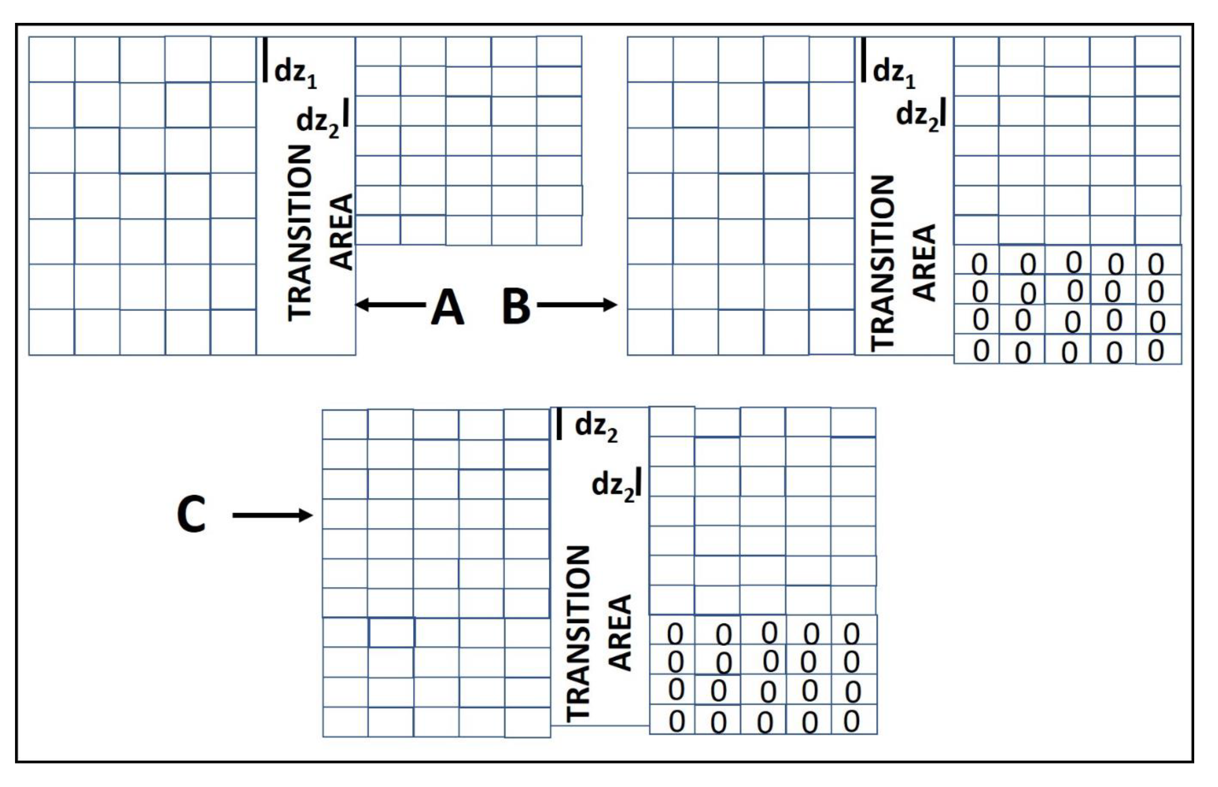
where dz₂ is the depth step for x>x₂ and is given by dz₂=0.5v₂dt, with dt being the time step of the data in the (x,t) domain. Eq. 3 involves of course an approximation intrinsic in the discretization (or sampling) of a continuous function of two variables represented by means of a matrix. At this point, we consider that the first (x<x₁) and second (x>x₂) part of the image represent the same spatial range, but of course the second part of the image (x>x₂) is represented by means a number of rows larger than the first part (x<x₁). This reflects the fact that the spatial step in the first part of the Bscan is given by dz₁=0.5v₁dt, which of course is larger than dz₂. The problem is solved by simply resampling the columns of the first part of the image. In particular, if N is the original number of rows of the Bscan, then each column of the first part of the migrated image has to be resampled from N to N+ΔN elements, with ΔN being given in Equation (3), which corresponds to resampling the first part of the migrated image with a depth step dz₂ instead of its original depth step dz₁. The passages are synoptically described in Figure 1.

At this point, we have to consider the transition area between the abscissas x₁ and x₂. We can deal with this zone in the same way that the two areas with a fixed value of velocity were treated, but acting column by column. In fact, from the transition of images that has generated the combined migration (Equation (1)), it is implicit that we have considered at any abscissa x in the transition zone a propagation velocity equal to

$$v\left(x\right)=\frac{\left(x_2-x\right)}{\left(x_2-x_1\right)}{v}_1+\frac{\left(x-x_1\right)}{\left(x_2-x_1\right)}{v}_2$$

(8)

Consequently, in the migrated image, the column corresponding to the abscissa x, after time-depth conversion according to the propagation velocity v=v(x), reaches a maximum depth equal to z_maxx=0.5v(x)T_max and therefore has to be zero-padded up to the depth level z_max1=0.5v₁T_max accounting for its own depth step dz_x=0.5v(x)dt. This amounts to adding to the current column in the transition area a number of null elements equal to

$$\Delta N_x=round\left(\frac{z_{max1}-z_{maxx}}{d{z}_x}\right)=round\left[\frac{\left(v_1-v\left(x\right)\right)T_{max}}{v\left(x\right)dt}\right]$$

(9)

Afterwards, the column has to resampled from N+ΔN_x to N+ΔN elements to report its original depth step dz_x to dz₂. The comprehensive result will be a zero-padding progressively more intense from x₁ to x₂ and a resampling progressively less intense from x₁ to x₂. After the combined time-depth conversion, the bottom of the resulting matrix has some null parts. This is natural, because the depth reached by the signal is not the same from point to point. However, if one does not want to see such an effect, it is sufficient to take the time bottom scale beyond the time depth of interest, so that the bottom of the resulting matrix can be cut away because it does not contain relevant information.

2.2. Vertical Variations of v

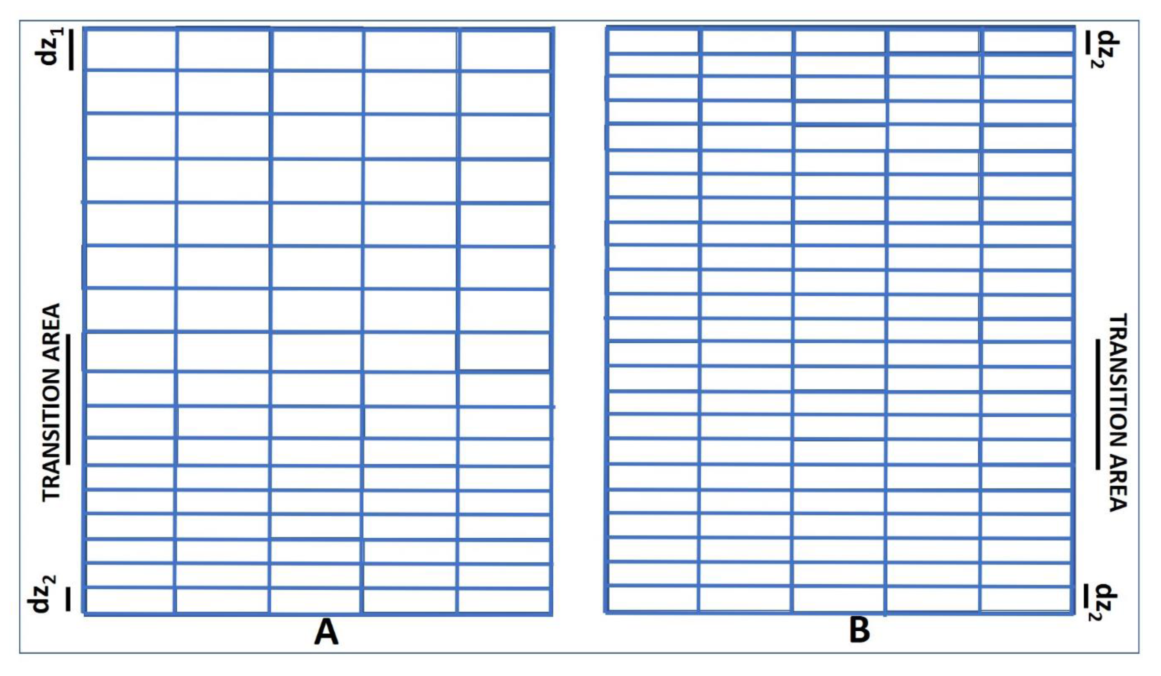
A synopsis of the time-depth conversion in the case of vertical variations of the propagation velocity is provided in Figure 2. In the case of vertical variations of the propagation velocity, no zero-padding is needed because the relevant pieces of matrixes are piled on each other and the comprehensive spatial bottom scale is just the sum of the partial spatial bottom scales relative to the three matrixes given by Im₁, Im₂ and the vertical transition area.

As can be appreciated in Figure 2, in the case of vertical variations of the propagation velocity, the combined time-depth conversion is slightly more complicated. In fact, the depth step dz along each column of the time-depth-converted migrated image is no longer constant. In fact, the propagation velocity of the electromagnetic waves in the vertical transition zone is now evaluated as

$$v\left(t\right)=\frac{\left(t_2-t\right)}{\left(t_2-t_1\right)}{v}_1+\frac{\left(t-t_1\right)}{\left(t_2-t_1\right)}{v}_2$$

(10)

and consequently we have dz=dz_t=0.5v(t)dt in the transition zone. This poses two problems. The first problem is related to the optimal choice of the position of the transition zone. In fact, this influences the resulting depth conversion of all the deeper levels. In the case of horizontal variations of v, this did not happen, and this was because the effects of the positioning of the horizontal transition area remained local. On the other hand, the case with vertical variation of v is often ascribable to a layered medium, with interfaces between the strata identifiable by eye from the data.

A second issue to account for is the variable depth step in the transition zone. To show this, suppose again v₁>v₂ (again, the treatment in the case v₂>v₁ is straightforwardly deduced). In the upper part of the matrix, corresponding to t<t₁, the resulting vertical step is dz₁=0.5v₁dt, and the corresponding spatial thickness of this piece of Bscan is given by Δz₁=0.5v₁t₁. In the lower part of the Bscan, corresponding to t>t₂, the resulting depth step is given by dz₂=0.5v₂dt, and the comprehensive thickness of this piece of image is given by Δz₂=0.5v₂(T_max-t₂). We have to resample the upper part of the Bscan so that its initial depth step dz₁ is reduced to dz₂. Labeling the initial number of rows of this upper part of the Bscan as M (resulting in M=1+round(Δz₁/dz₁)), we easily work out that we have to resample these M values into M+ΔM, where

$$\Delta M=round\left(\frac{\Delta z_1}{d{z}_2}\right)-round\left(\frac{\Delta z_1}{d{z}_1}\right)$$

(11)

With regard to the time-depth conversion in the vertical transition zone, it should be done with a progressively more intense resampling because the depth step decreases linearly from dz₁ to dz₂ when t ranges from t₁ to t₂. The computation of the resampling needed in order to have an optimal time-depth conversion is not a straightforward operation, but we can reasonably assume that the transition zone is not much extended in terms of internal wavelength, so that any deformation of the targets deriving from a non-optimal time domain conversion in this vertical belt is negligible. Under this hypothesis, we can adopt an approximated algorithm, wherein first the comprehensive thickness Δz_tr of the vertical transition area is evaluated. Then, the depth range Δz_tr is divided into K parts so that the length of each depth interval is (within the available precision due to the quantization) about equal to dz₂. The theoretical comprehensive depth range relative to the transition area is given in the following formula:

$$\Delta z_{tr}=0.5{{\displaystyle \int }}_{t_1}^{t_2}v\left(t\right)dt$$

(12)

From a practical point of view, Δz_tr is the sum of the thicknesses relative to each row in the transition zone. The number of rows K into which the transition zone has to be resampled is given by

$$K=round\left(\frac{\Delta z_{tr}}{d{z}_2}\right)$$

(13)

The lower part of the image remains as it is. Suppose now that it is composed of M₁ rows. After implementing the described resampling, the comprehensive number of rows of the resulting image in the (x,z) domain is given by M+ΔM+K+M₁, and the spatial bottom scale to impose to the image is given by z_max=Δz₁+ Δz_tr+Δz₂.

In the case (indeed quite rare) that a more refined time-depth conversion in the vertical transition area is needed, it is possible to adopt a procedure in two or more steps. Limiting to the case of two steps, we can consider a time range from t₁ up to 0.5(t₁+t₂) and another one starting from 0.5(t₁+t₂) and extending up to t₂. The vertical extensions in the (x,z) domain of the upper and lower transient zones Δz_tru and Δz_trl are respectively given by

$$\left\{\begin{array}{c}\Delta z_{tru}=0.5\underset{t_1}{\overset{\frac{t_1+t_2}{2}}{{\displaystyle \int }}}v\left(t\right)dt\\ \Delta z_{trl}=0.5\underset{\frac{t_1+t_2}{2}}{\overset{t_2}{{\displaystyle \int }}}v\left(t\right)dt\end{array}\right.$$

(14)

Then, the upper and lower transition zones can be separately resampled so that the medium depth step becomes about equal to dz₂ for both of them. Of course, this reduces the distortion within transition zone. For the calculation of the maximum depth range, now we can consider Δz_tru+ Δz_trl= Δz_tr and achieve, similarly to before, z_max=Δz₁+Δz_tr+Δz₂. Of course, Δz_tru and Δz_trl are not equal to each other.

3. Measurement Setup

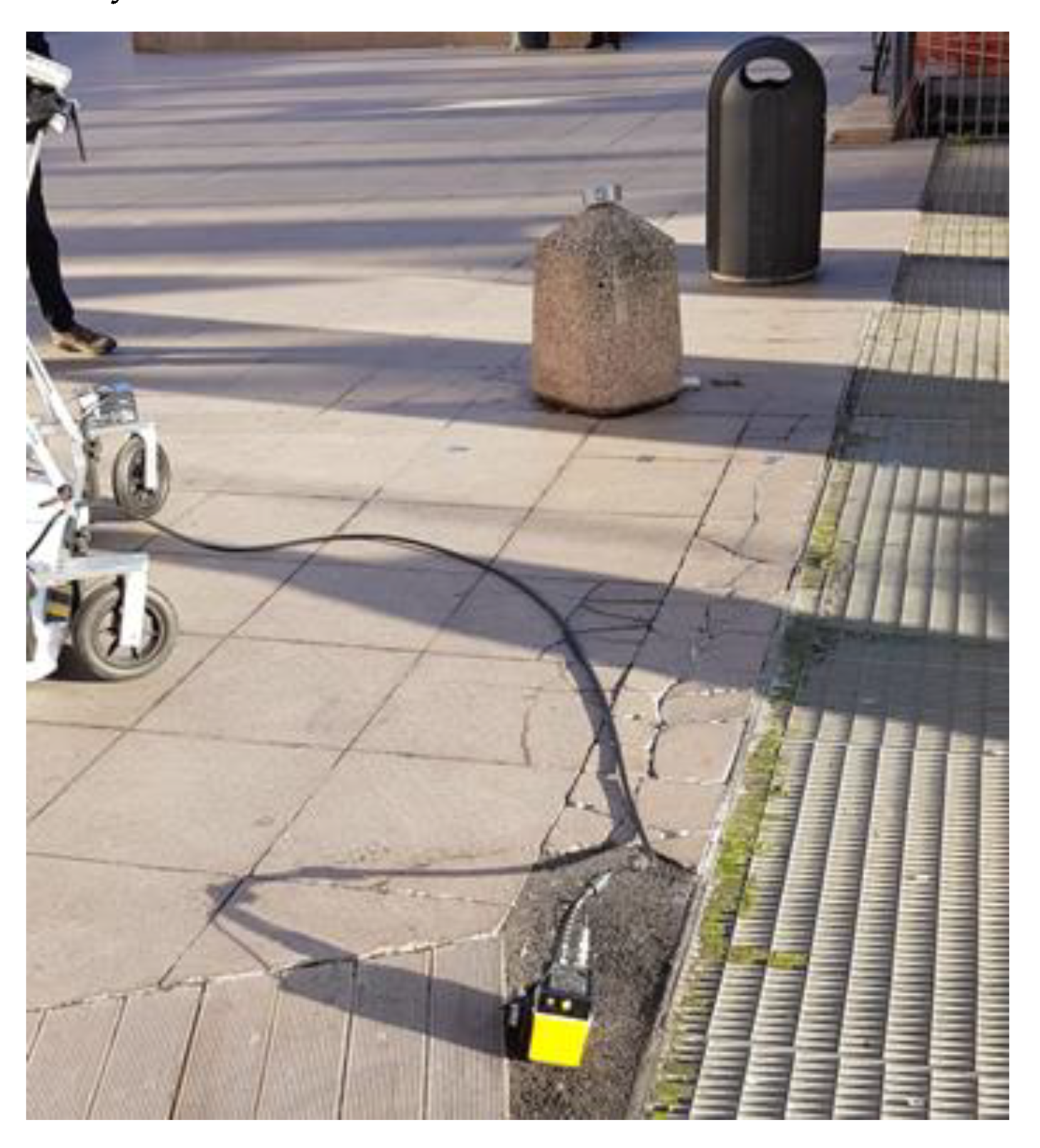
We will present here two Bscans extracted from a large GPR measurement campaign performed by Geostudi Astier Ltd. The measurements were taken in a square covered with concrete, where some water infiltrations were supposed. The square is for pedestrians, so no asphalted zone is present. A large part was prospected with a system equipped with an array of antennas that also allowed the retrieval of time slices, but they are not considered here. Several isolated Bscans (more than 30) close to particular points, particularly suspected of water infiltrations, were prospected with a single antenna system, namely a RIS Hi-mode GPR equipped with an antenna at 3 GHz. In Figure 3, a photo of the equipment is shown. The applied bottom scale was 15 ns, and the number of time samples was 256, so that the time step was 0.0547 ns. The spatial step (imposed with an odometer) was 6 mm, so that the number of traces per meter was 167. The processing was essentially constituted by zero timing, possible background removal, gain vs. depth and 1D filtering, plus the migrations and the combination of the migrations. However, the chosen processing parameters were case-dependent and will be described case by case in the next section.

4. Results

4.1. Horizontal Variations of the Propagation Velocity

Let us now show a case with horizontal variations of the propagation velocity of the waves.

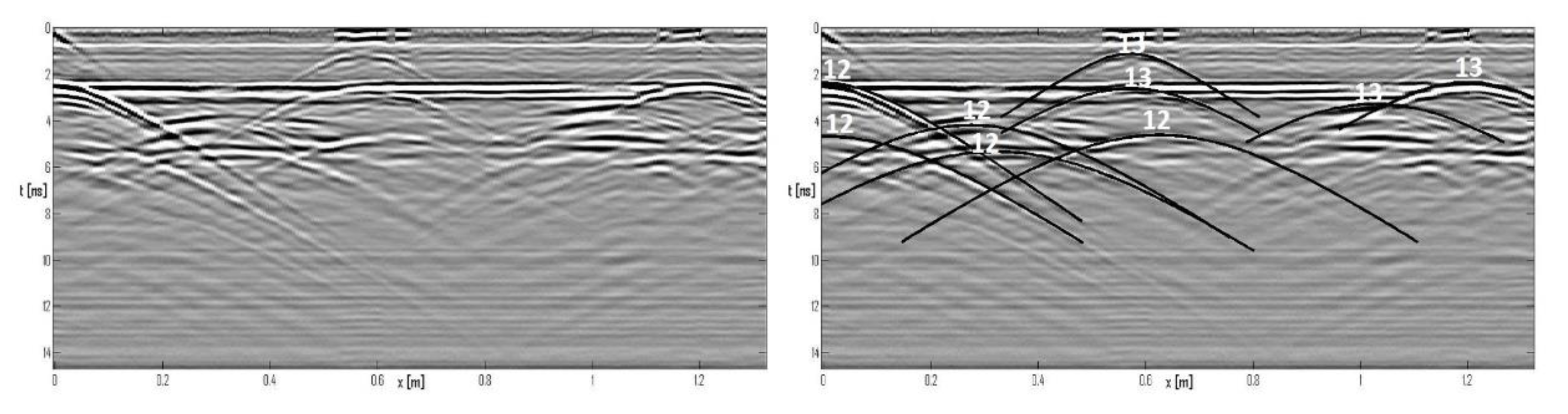
In Figure 4, data that were preprocessed but not migrated are shown. The data were processed by means of the Reflexw commercial code, and the processing steps were a time zero at 1.29 ns and a background removal limited to the two time intervals 0–0.5 ns and 2–2.8 ns in order to clean some disturbances due to the air–concrete interface and to a layer visible around the time level of 2.5 ns, respectively. Limiting the background removal to these intervals, moreover, prevented spurious anomalies from arising due to this processing step when strong concentrated reflectors are present. Afterwards, linear and exponential gain were applied (the gain parameters were set to 1 and 2, respectively). Then, a Butterworth filtering with lower and upper cut frequencies of 500 and 6000 MHz, respectively, was applied.

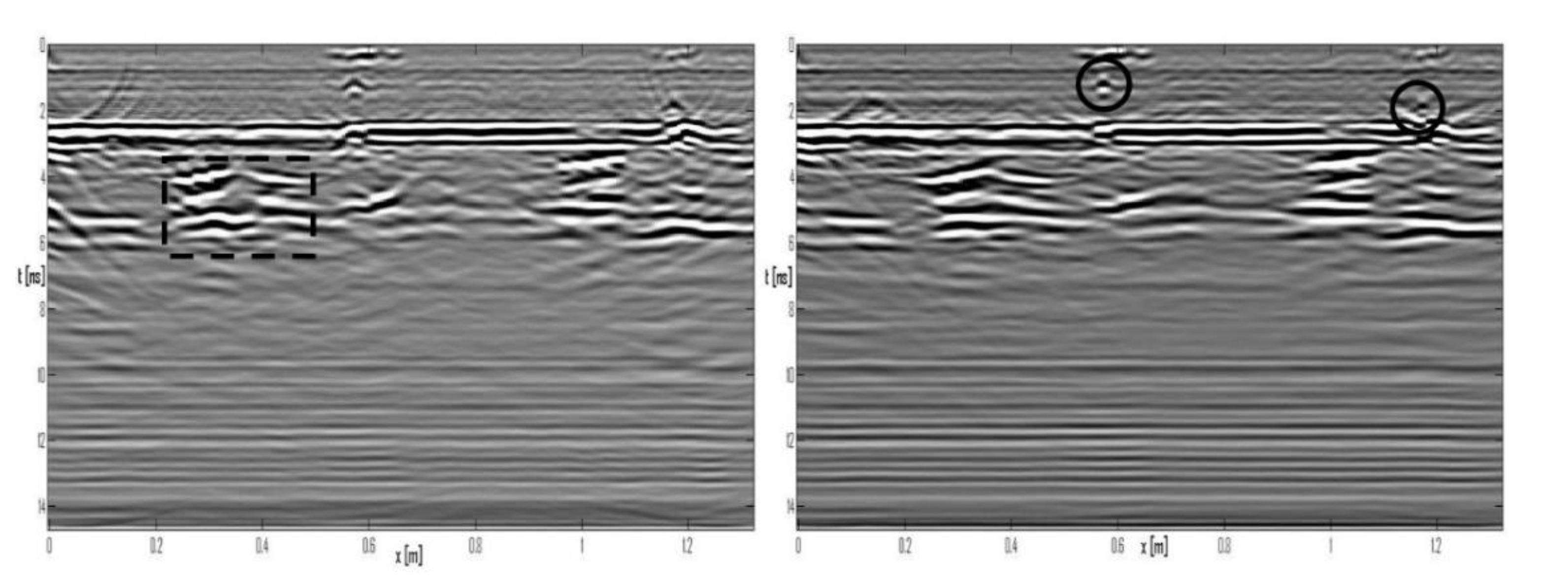
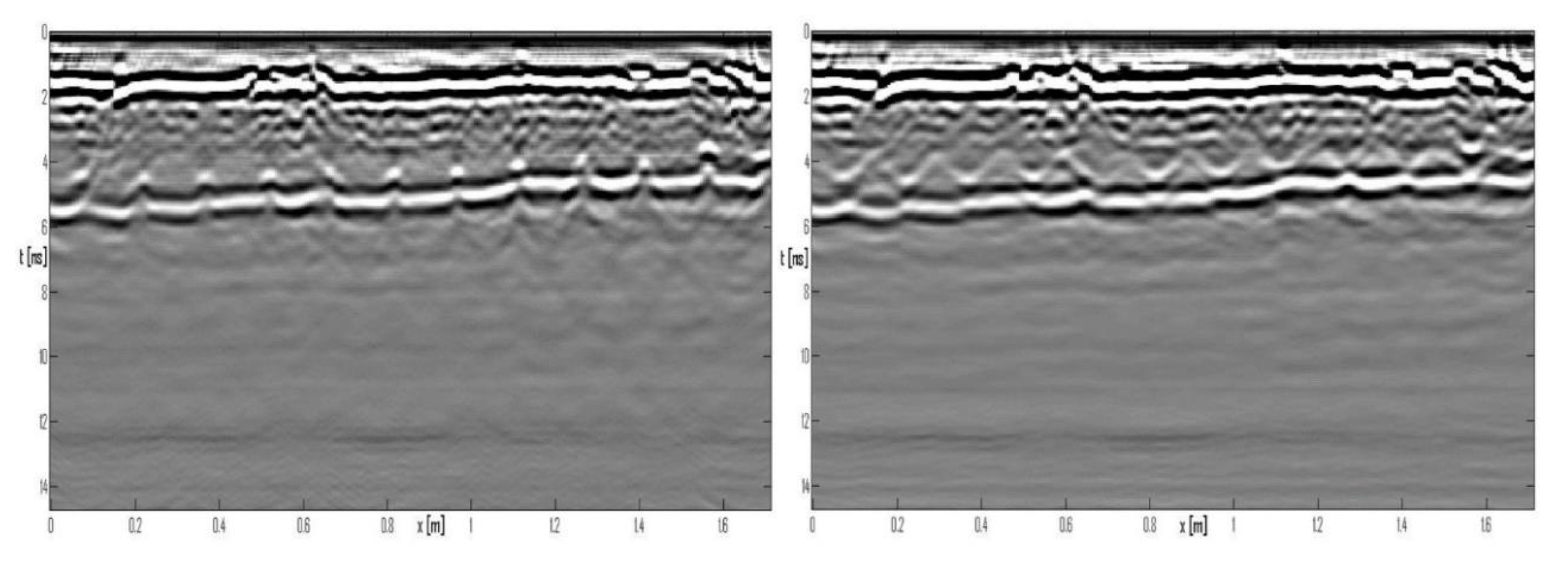
As can be seen from Figure 5, the migrated data show a substantial difference in the propagation velocity before and after the abscissa x=45 cm. The initial part of the image probably shows the effect of a higher percentage of moisture. The data were migrated twice, applying the Kirchhoff migration algorithm in time domain [11]. Two propagation velocity values equal to v₁=12 cm/ns and v₂=13 cm/ns were exploited for migrating the data. On the basis of the shape and length of the different diffraction hyperbolas, 81 traces were exploited for the migration with v=v₁=12 cm/ns, and 41 traces were exploited for the migration performed with v=v₂=13 cm/ns.

In Figure 5, the migration results are shown. As can be seen, the targets placed before the abscissa at 0.4 m appear more focused making use of the value v=v₁ (see the rectangle in the left-hand panel), and the targets displaced after the abscissa at 0.4 m appear more focused making use of the value v=v₂ (see the circles in the right-hand panel). In particular, in the left-hand panel, the two small targets at about 0.58 and 1.18 m appear as two frowns [19], which is the typical effect of an underestimation of the propagation velocity.

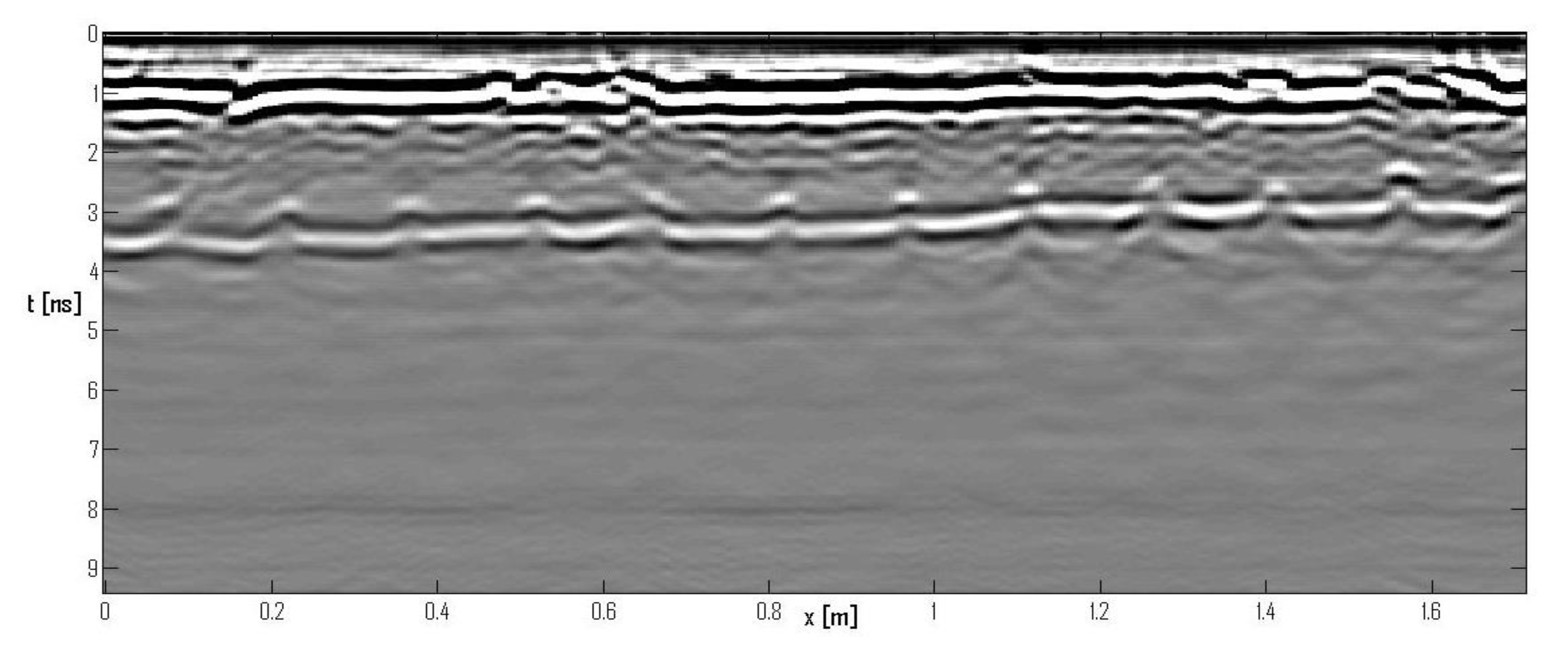
The two results of Figure 5 have been combined in Figure 6, with a linear transition between the left-hand and the right-hand images imposed in the abscissa range 40-54 cm. The data were also cut at the depth level 9.4 ns, beyond which, as it is quite clear from Figure 6, we essentially see the amplified ringing [21] of the antennas. The joining was implemented with a homemade code written in MATLAB environment. In particular, the data were exported to MATLAB in ASCII format.

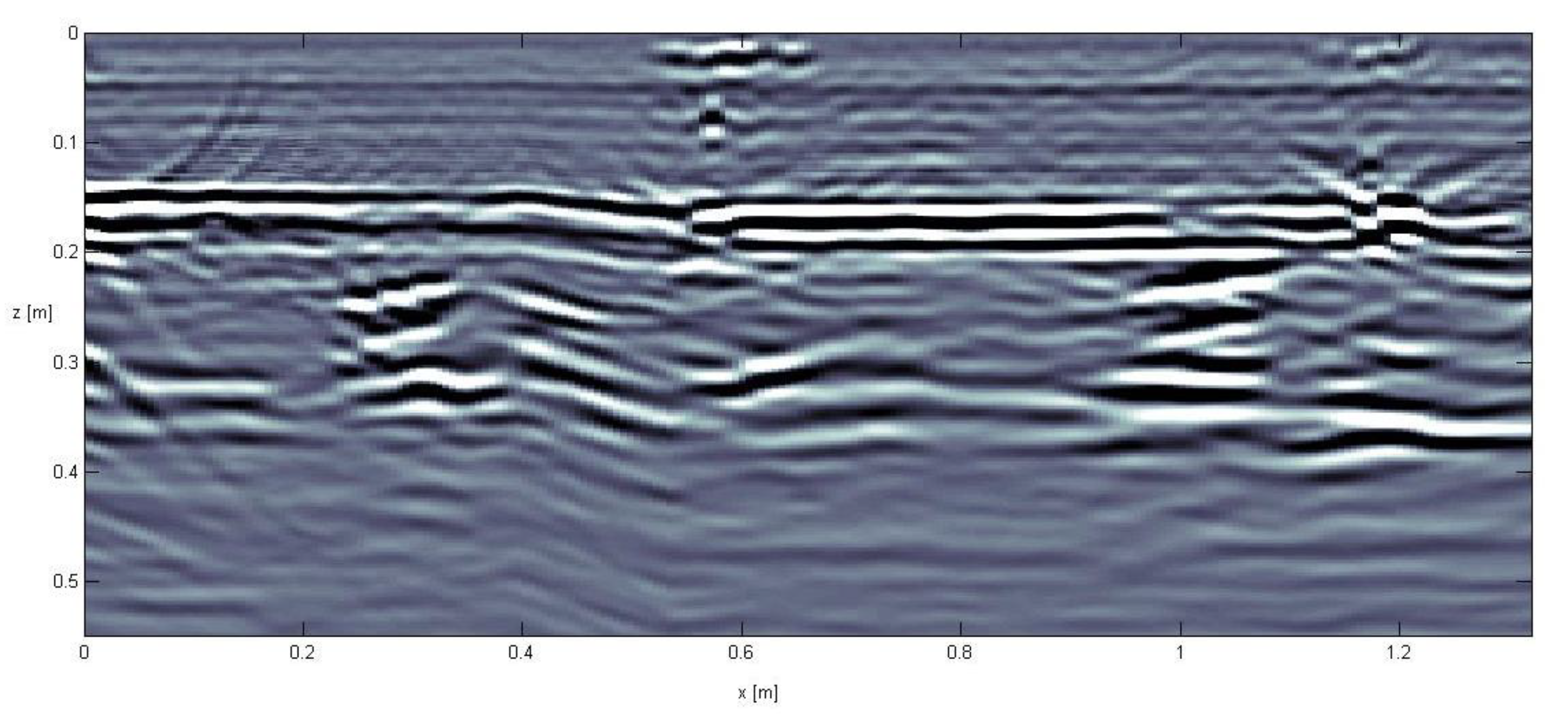
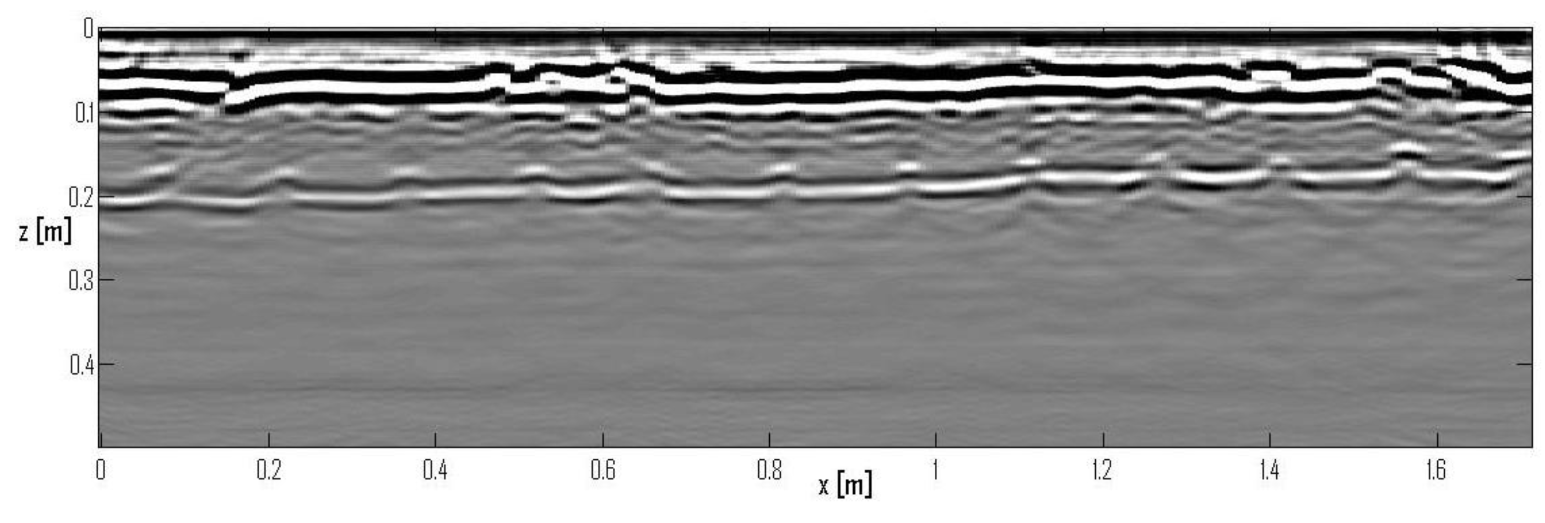
In Figure 7, the joined time-depth conversion relative to the combined migration of Figure 6 is shown. In Figure 7, the spatial proportions between abscissa and depth are respected. The zero-padding needed to construct Figure 7 does not appear, because it happens beyond the represented maximum depth level, which is 61 cm and corresponds (in relationship with v=v₂) to 9.4 ns. The anomaly at the depth of about 17 cm is probably a plastic liner.

4.2. Vertical Variations of the Propagation Velocity

Let us now show a case with a vertical transition of the propagation velocity. The data were gathered within the same measurement campaign from which we have extracted the previous image.

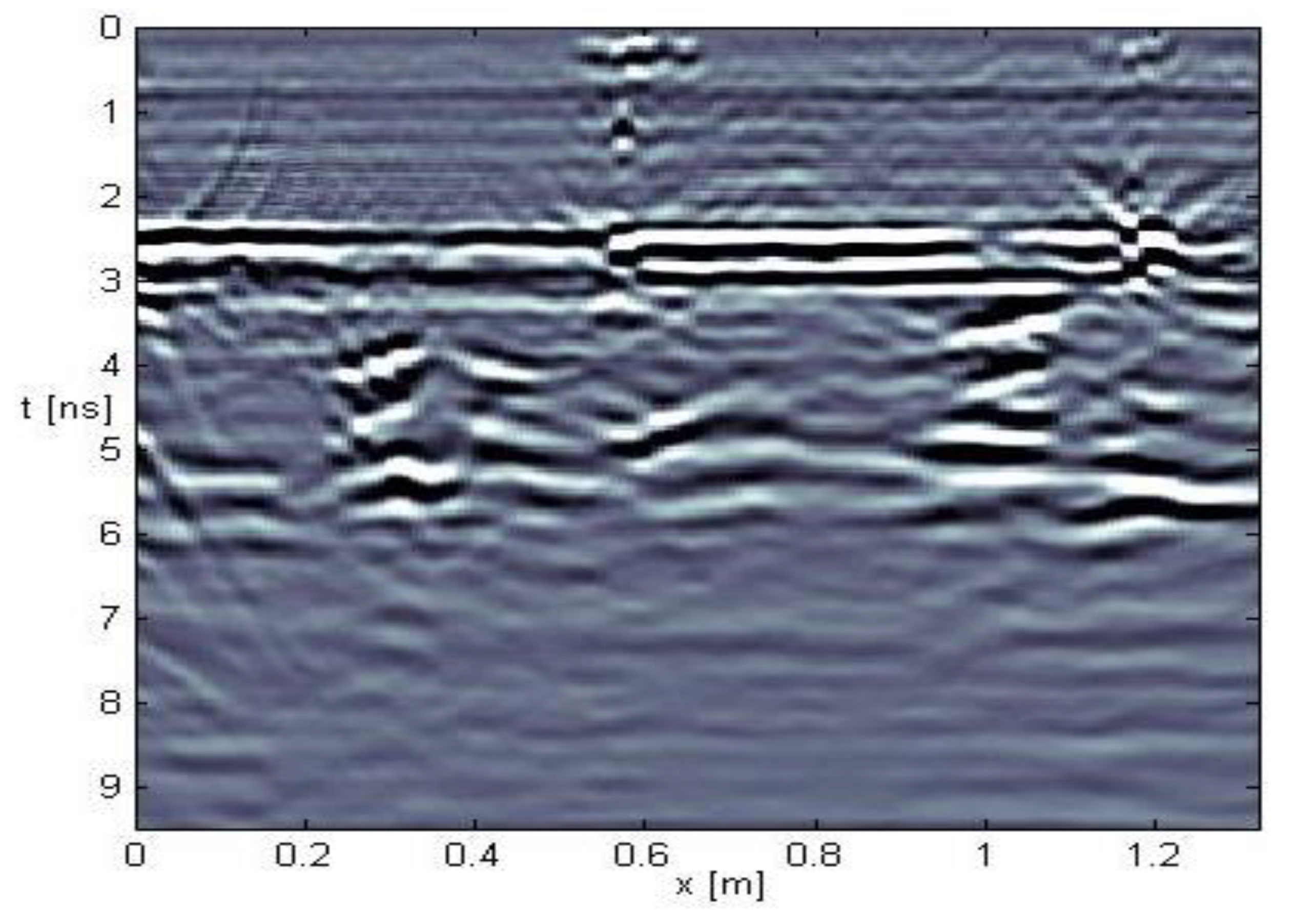
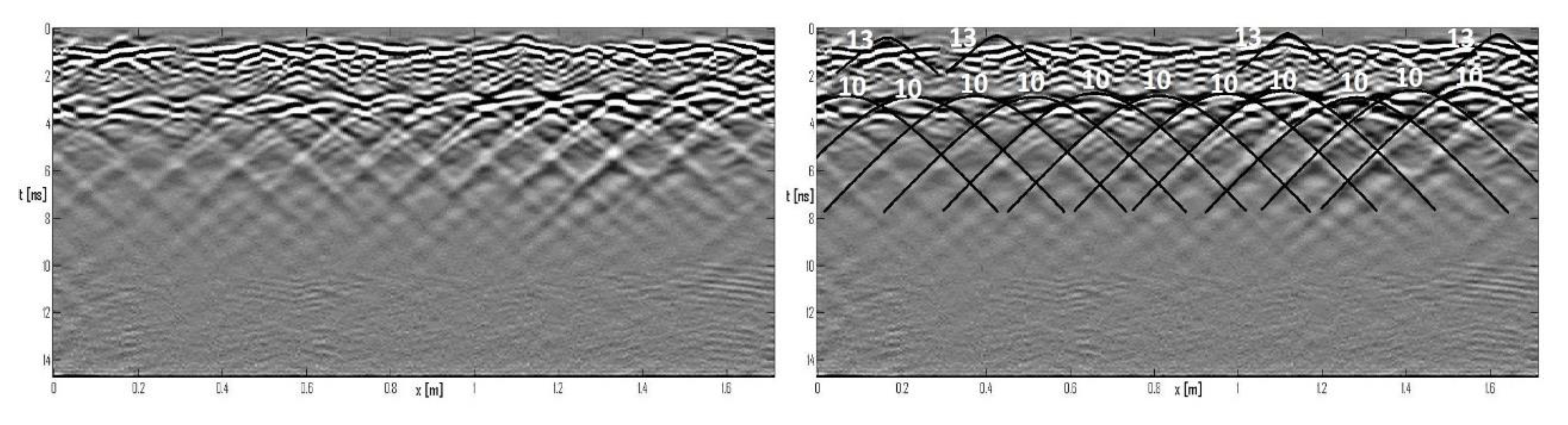
In this case, there is a sequence of bars (the material under consideration is reinforced concrete) and there are two alleged plastic liners. We implemented a preliminary preprocessing aimed to better identify the diffraction hyperbolas in order to better estimate the propagation velocity and the number of traces best advised for the migration processing. In order to do this, we applied time zero at 1.3 ns and subtracting average (bkg removal on a shifting interval) for 25 traces. Then, linear and exponential gain (with the chosen parameters of 2 and 3) and a Butterworth filtering between 500 and 6000 MHz were applied. We achieved the result shown in Figure 8, which makes the diffraction hyperbolas relative to reinforcing bars quite clear but partially obliterates the liners, especially the lower one. On the basis of the result of Figure 8, we identify a higher value of the propagation velocity for the shallower depth levels (about 13 cm/ns) and a lower value of the propagation velocity of the lower layers (about 10 cm/ns). This evaluation is not rigorous because, as said, the refraction of the waves between the superposed layers is neglected, but in the case at hand this is not a severe approximation because the upper layer is quite shallow. The upper (very shallow) hyperbolas are extended for about 21 traces, whereas the lower hyperbolas are extended for about 61 traces.

In Figure 9, the two migrated data sets are shown. For achieving this result, we restarted from the raw data and applied time zero at 1.3 ns, automatic gain control (AGC) with a factor 5 and Butterworth filtering with cut frequencies 500 and 6000 MHz. No kind of background removal was applied, in order to keep the liners, i.e., the anomalies of interest, visible. Following this, Kirchhoff migration was first applied with v=v₁=10 cm/ns and the use of 61 traces and then applied with v=v₂=13 cm/ns and the use of 41 traces.

From Figure 9, we can appreciate that by setting v=v₁=10 cm/ns, the sequence of bars at the time level of about 3 ns is better focused, whereas some shallow anomalies at about 1 ns are better focused by setting v=v₂=13 cm/ns (see in particular in abscissa range 0.4-0.8 m).

In Figure 10, a joined migration merging the two panels of Figure 9 is shown. A vertical transition area in the time range 1.6-2 ns has been adopted for this.

In Figure 11, the time-depth conversion is shown. Figure 11 shows the correct proportions between abscissa and depth.

5. Conclusions

In this paper, we have presented the possibility to combine migration results achieved with different values of the propagation velocity of the electromagnetic waves in the medium at hand, in the case of a horizontally variable medium and the case of a vertically variable medium. The approach is intended for practical purposes; it is a simple way to improve achieved results while using commercial processing codes for focusing. However, the approach has also its own limits. While, in particular, it can present more delicate aspects in the case of a vertically layered medium, it can make it possible to achieve a better focusing and a better time-depth conversion with respect to the choice of a unique “average” propagation velocity of the electromagnetic waves. The adoption of a transition zone between the areas with different propagation velocities instead of imposing an abrupt change allows avoiding seams in the final image.

A question about the optimal positioning of the transition zone arises. The answer to this question can be simple or more complex depending on the case. Indeed there are two possibilities: the case when a sharp discontinuity is visible in the data (e.g., the case of a layered medium) and the case when we only see different values of velocity associated to different diffraction hyperbolas. In the first case, the answer is immediate (and the extent of the transition zone reduces to zero). In the second case, there is indeed some degree of arbitrariness in placing the transition zone (or zones). However, it is clear that a reasonable criterion is to displace it in a spatial range where no relevant target is visible. In this case, the effect of the precise position of the transition zone will be unimportant in the case of horizontal variations of the propagation velocity, whereas it shall be heuristically chosen in the case of vertical variations, being aware that its position will influence the estimation of the depth of all the deeper targets.

The scope of this study was limited to considering the diffraction hyperbolas as the way to measure the propagation velocity. Of course, there are further evaluation methods, e.g., common midpoint data [22], TDR measurements [23,24], localised excavation tests [25] or, if available, the use of some cooperative target at known depth [26]. These methods, especially with regard to the deeper strata of a layered medium, can provide a more reliable measurement of the propagation velocity. If this is the case, even if the exploited migration procedure is not optimal, the presented combined time-depth conversion algorithm is certainly more reliable than any “average” value of the propagation velocity.

It is possible that the Bscan requires two or more transitions (either horizontal or vertical). These can be implemented in a relatively straightforward way and will be the object of future study.

Further future developments will regard the possible application of both horizontal and vertical transitions in the same image, as well as the application of the combined migrations to several adjacent images, in order to have the possibility to achieve more significant depth slices [27,28] constructed directly in the spatial domain after a sequence of combined time-depth conversions.

References

- Greaves, R.J.; Lesmes, D.P.; Lee, J.M.; Toksoz, M.N. Velocity variations and water content estimated from multi-offset, ground-penetrating radar. Geophysics 1996, 61, 683–695. [Google Scholar] [CrossRef]
- Hugenschmidt, J.; Loser, R. Detection of Chlorides and Moisture in Concrete Structures with GPR. Mater. Struct. Mater. Constr. 2008, 41, 785–792. [Google Scholar] [CrossRef] [Green Version]
- Chang, W.C.; Lin, C.H.; Lien, H.S. Measurement radius of reinforcing steel bar in concrete using digital image GPR. Constr. Build. Mater. 2009, 23, 1057–1063. [Google Scholar] [CrossRef]
- Jol, H. Ground Penetrating Radar: Theory and Applications; Elsevier: Amsterdam, The Netherlands, 2009. [Google Scholar]
- Persico, R.; Leucci, G.; Matera, L.; De Giorgi, L.; Soldovieri, F.; Cataldo, A.; Cannazza, G.; De Benedetto, E. Effect of the height of the observation line on the diffraction curve in GPR prospecting. Near Surface Geophys. 2015, 13, 243–252. [Google Scholar] [CrossRef]
- Mertens, L.; Persico, R.; Matera, L.; Lambot, S. Smart automated detection of reflection hyperbolas in complex GPR images With No A Priori Knowledge on the Medium. IEEE Trans. Geos. Rem. Sens. 2016, 54, 580–596. [Google Scholar] [CrossRef]
- Yuan, H.; Montazeri, M.; Looms, M.C.; Nielsen, L. Diffraction imaging of ground-penetrating radar data. Geophysics 2019, 84, H1–H12. [Google Scholar] [CrossRef]
- Persico, R.; Soldovieri, F. Effects of the Background Removal in Linear Inverse Scattering. IEEE Trans. Geosci. Remote Sens. 2008, 46, 1104–1114. [Google Scholar] [CrossRef]
- Allroggen, N.; Tronicke, J.; Boniger, D.U. Topographic migration of 2D and 3D ground-penetrating radar data considering variable velocities. Near Surf. Geophys. 2015, 8, 253–259. [Google Scholar] [CrossRef]
- Stolt, R.H. Migration by Fourier Transform. Geophysics 1978, 43, 23–48. [Google Scholar] [CrossRef]
- Schneider, W.A. Integral formulation for migration in two and three dimensions. Geophysics 1978, 43, 49–76. [Google Scholar] [CrossRef]
- Persico, R. Introduction to Ground Penetrating Radar: Inverse Scattering and Data Processing; Wiley-IEEE Press: Hoboken, NJ, USA, 2014. [Google Scholar]
- Lesselier, D.; Duchene, B. Wavefield inversion of objects in stratified environments: From back-propagation schemes to full solutions. In Review of Radio Science 1993–1996; Stone, R., Ed.; Oxford University Press: Oxford, UK, 1996. [Google Scholar]
- Meincke, P.; Hansen, T.B. Plane wave characterization of antennas close to a plane interface. IEEE Trans. Geos. Rem. Sens. 2004, 42, 1222–1232. [Google Scholar] [CrossRef]
- Muller, P.; Schurmann, M.; Guck, J. The Theory of Diffraction Tomography; Cornell University: Ithaca, NY, USA, 2016. [Google Scholar]
- Schofield, J.; Danield, D.; Hammerton, P. A multiple migration and stacking algorithms designed for land mine detection. IEEE Trans. Geosci. Remote Sens. 2014, 52, 6983–6988. [Google Scholar] [CrossRef] [Green Version]
- Huo, J.; Zhao, Q.; Zhou, B.; Liu, L.; Ma, C.; Guo, J.; Xie, L. Energy flow domain reverse-time migration for borehole radar. IEEE Trans. Geosci. Remote Sens. 2019, 57, 7221–7231. [Google Scholar] [CrossRef]
- Zhang, F.; Liu, B.; Liu, L.; Wang, J.; Lin, C.; Yang, L.; Li, Y.; Zhang, Q.; Yang, W. Application of ground penetrating radar to detect tunnel lining defects based on improved full waveform inversion and reverse time migration. Near Surf. Geophys. 2019, 17, 127–139. [Google Scholar] [CrossRef]
- De Smet, T.S.; Everett, M.E.; Warden, R.R.; Komas, T.; Hagin, J.N.; Gavette, P.; Martini, J.A.; Barker, L. The fate of the historic fortifications at Alcatraz Island based on terrestrial scans and ground-penetrating radar interpretations from the recreation yard. Near Surf. Geophys. 2019, 17, 151–168. [Google Scholar] [CrossRef]
- Sala, J.; Linford, N. Processing stepped frequency continuous wave GPR system so to obtain maximum value from archaeological data sets. In Proceedings of the XIII Internarional Conference on Ground Penetrating Radar, Lecce, Italy, 21–25 June 2010; Volume 10, pp. 1–6, ISBN 978-1-4244-4605-6. [Google Scholar]
- Gao, X.; Podd, F.J.W.; van Verre, W.; Daniels, D.J.; Peyton, A.J. Investigating the Performance of Bi-Static GPR Antennas for Near-Surface Object Detection. Sensors (Basel) 2019, 19, 179. [Google Scholar] [CrossRef] [Green Version]
- Dix, C.H. Seismic velocities from surface measurements. Geophysics 1955, 20, 68–86. [Google Scholar] [CrossRef]
- Persico, R.; Pieraccini, M. Measurement of dielectric and magnetic properties of Materials by means of a TDR probe. Near Surf. Geophys. 2018, 16, 1–9. [Google Scholar] [CrossRef]
- Farhat, I.; Farrugia, L.; Persico, R.; D’Amico, S.; Sammut, C. Preliminary Experimental Measurements of the Dielectric and Magnetic Properties of a Material with a Coaxial TDR Probe in Reflection Mode. Prog. Electromagn. Res. 2020, 91, 111–121. [Google Scholar] [CrossRef]
- Goodman, D.; Piro, S. GPR Remote Sensing in Archaeology; Springer: Berlin/Heidelberg, Germany, 2013. [Google Scholar]
- Soldovieri, F.; Prisco, G.; Persico, R. Application of Microwave Tomography in Hydrogeophysics: Some examples. Vadose Zone J. 2008, 7, 160–170. [Google Scholar] [CrossRef]
- Matera, L.; Noviello, M.; Ciminale, M.; Persico, R. Integration of multisensor data: An experiment in the archaeological park of Egnazia (Apulia, Southern Italy). Near Surf. Geophys. 2015, 13, 613–621. [Google Scholar] [CrossRef]
- Persico, R.; D’Amico, S.; Matera, L.; Colica, E.; De Giorgio, C.; Alescio, A.; Sammut, C.; Galea, P. GPR Investigations at St John’s Co-Cathedral in Valletta. Near Surf. Geophys. 2019, 17, 213–229. [Google Scholar] [CrossRef]
Figure 1.
Pictorial synopsis for horizontal velocity transition: Image A represents the initial situation after separate time-depth conversions. Image B represents the situation after zero-padding of the area with slower propagation velocity. Image C shows the situation after resampling the part with faster propagation velocity.
Figure 2.
Pictorial synopsis for vertical velocity transition: Image (A) represents the initial situation after separate time-depth conversion. Image (B) represents the situation after resampling of the part with faster propagation velocity and the transition area.
Figure 3.
A photograph of the exploited GPR antenna.
Figure 4.
Pre-migrated data. The Bscan is the same on the left-hand and on the right-hand panel. On the right-hand side, model diffraction hyperbolas are superposed on the data to match them. The procedure is manual. The numbers on the hyperbolas indicate the trial propagation velocity in cm/ns.
Figure 5.
Migrated data. Left-hand panel: v=v1=12 cm/ns. Right-hand panel: v=v2=13 cm/ns.
Figure 6.
Joined migration with horizontal variation of the propagation velocity, merging the results of Figure 4.
Figure 7.
Joined time-depth conversion with horizontal variation of the propagation velocity, related to the result of Figure 6.
Figure 8.
Pre-migrated data. The applied processing was intended to make the diffraction hyperbolas clearer. The Bscan is the same on the left- and right-hand panels. On the right-hand side, model diffraction hyperbolas are superposed to the data so as to match them. The procedure is manual. The numbers on the hyperbolas indicate the trial propagation velocity in cm/ns.
Figure 9.
Migrated data. Left-hand panel: v=v1=10 cm/ns and 61 traces involved in the migration process. Right hand panel: v=v2=13 cm/ns and 41 traces involved in the migration process.
Figure 10.
Joined migration with vertical variation of the propagation velocity, merging the results of Figure 8.
Figure 11.
Joined time-depth conversion with vertical variation of the propagation velocity, related to the result of Figure 10.
© 2020 by the authors. Licensee MDPI, Basel, Switzerland. This article is an open access article distributed under the terms and conditions of the Creative Commons Attribution (CC BY) license (http://creativecommons.org/licenses/by/4.0/).
Share and Cite
MDPI and ACS Style
Persico, R.; Morelli, G. Combined Migrations and Time-Depth Conversions in GPR Prospecting: Application to Reinforced Concrete. Remote Sens. 2020, 12, 2778. https://0-doi-org.brum.beds.ac.uk/10.3390/rs12172778
AMA Style
Persico R, Morelli G. Combined Migrations and Time-Depth Conversions in GPR Prospecting: Application to Reinforced Concrete. Remote Sensing. 2020; 12(17):2778. https://0-doi-org.brum.beds.ac.uk/10.3390/rs12172778
Chicago/Turabian StylePersico, Raffaele, and Gianfranco Morelli. 2020. "Combined Migrations and Time-Depth Conversions in GPR Prospecting: Application to Reinforced Concrete" Remote Sensing 12, no. 17: 2778. https://0-doi-org.brum.beds.ac.uk/10.3390/rs12172778
Note that from the first issue of 2016, this journal uses article numbers instead of page numbers. See further details here.