Deep Hash Remote Sensing Image Retrieval with Hard Probability Sampling


1
College of Computer Science and Technology, Jilin University, Changchun 130012, China
2
Key Laboratory of Symbolic Computation and Knowledge Engineering of Ministry of Education, Jilin University, Changchun 130012, China
3
School of Mechanical Science and Engineering, Jilin University, Changchun 130025, China
4
College of Communication Engineering, Jilin University, Changchun 130012, China
5
School of Computer Science and Technology, Shandong University of Technology, Zibo 255000, China
*
Author to whom correspondence should be addressed.
Remote Sens. 2020, 12(17), 2789; https://0-doi-org.brum.beds.ac.uk/10.3390/rs12172789
Submission received: 15 July 2020
/
Revised: 19 August 2020
/
Accepted: 25 August 2020
/
Published: 27 August 2020
(This article belongs to the Special Issue Content-Based Remote Sensing Image Retrieval)
Abstract
:As satellite observation technology improves, the number of remote sensing images significantly and rapidly increases. Therefore, a growing number of studies are focusing on remote sensing image retrieval. However, having a large number of remote sensing images considerably slows the retrieval time and takes up a great deal of memory space. The hash method is being increasingly used for rapid image retrieval because of its remarkably fast performance. At the same time, selecting samples that contain more information and greater stability to train the network has gradually become the key to improving retrieval performance. Given the above considerations, we propose a deep hash remote sensing image retrieval method, called the hard probability sampling hash retrieval method (HPSH), which combines hash code learning with hard probability sampling in a deep network. Specifically, we used a probability sampling method to select training samples, and we designed one novel hash loss function to better train the network parameters and reduce the hashing accuracy loss due to quantization. Our experimental results demonstrate that HPSH could yield an excellent representation compared with other state-of-the-art hash approaches. For the university of California, merced (UCMD) dataset, HPSH+S resulted in a mean average precision (mAP) of up to 90.9% on 16 hash bits, 92.2% on 24 hash bits, and 92.8% on 32 hash bits. For the aerial image dataset (AID), HPSH+S achieved a mAP of up to 89.8% on 16 hash bits, 93.6% on 24 hash bits, and 95.5% on 32 hash bits. For the UCMD dataset, with the use of data augmentation, our proposed approach achieved a mAP of up to 99.6% on 32 hash bits and 99.7% on 64 hash bits.
1. Introduction
With the improvement in satellite observation technology, the number of remote sensing images has significantly and rapidly increased [1,2]. This aspect has motivated many researchers to focus on applications of remote sensing images, such as recognition, detection, classification, and retrieval. Of the many processes involved, remote sensing image retrieval (RSIR) [3,4,5] is the most challenging. The primary task of RSIR is to return all images that are visually similar to the given query image in a retrieval dataset. Moreover, large collections of high-resolution remote sensing images are continuously emerging. Usually, these remote sensing (RS) images include a large range of geographical areas, and many of these areas contain a lot of semantic instances [6,7,8,9,10,11]. Establishing an optimal approach to building a remote sensing image system with high computational efficiency and accurate results has become the biggest challenge in remote sensing image retrieval research.
In RSIR [6,7,8,9,10,11], in order to enhance retrieval effectiveness, deep metric learning (DML) is frequently used to learn more representative high-level features, which are obtained through a convolutional neural network (CNN). DML is used to learn the embedding space, in which similar samples from the same category are pulled close to each other, and at the same time, dissimilar samples from different categories are kept apart [12,13,14]. Generally, the main operation of DML contains two aspects. The first is the selection of appropriate sample pairs during training. Sample pairs whose similarities are incorrectly represented in a particular embedded space tend to have higher contributions to the loss function calculation. These sample pairs are called informative samples in DML, and they lead to fast convergence. The second aspect is the design of effective loss functions. The pairwise loss function [15,16,17,18,19] is a typical choice in RSIR; it constructs pairwise samples for training, and examples include contrastive loss [15], triplet loss [16], lifted structured loss [17], ranked list loss [18], and margin-based loss [19]. Contrastive loss [15] does not take into account dissimilar pairs whose distance is smaller than the given margin. Triplet loss [16] is based on triplets, which means that the triplet selection is a significant step. It is more relaxed on the distance constraint between samples and is faster. Lifted structured loss [17] assigns larger weights to more informative samples. Margin-based loss [19] considers both distant positive pairs and close negative pairs. However, the random selection of redundant and less informative samples leads to slow convergence and can obtain inferior results.
Sample selection in DML [6,15,17,19,20,21,22,23,24] takes an equal or more significant position than loss functions. For example, in random sampling [15,20,21], no consideration is given to the distribution of samples that are drawn randomly. Hard negative mining uses a fixed boundary to select hard negative samples. Semi-hard negative mining [17,22] is widely adopted. This method jointly uses the anchor and a given positive sample to choose negative samples. Thus, it can provide hard but not too hard negative samples for training. The method for selecting informative samples is vital to network training. At the same time, the approach to organizing the training samples plays an equally important role. As has been proved in triplet loss [16], if hard mining is adopted, many images have the same embedding, and this ultimately leads to model collapse. This means that training samples cannot only consist of hard negative (positive) samples. Furthermore, most of the current mining methods involve uniform sampling and ignore the sample distribution. We attempt to utilize a hard negative probability sampling method to find more informative training samples while maintaining the samples’ diversity.
Usually, having a large number of RS images substantially increases retrieval time and takes up a great deal of memory space. Therefore, as a dimension reduction method, hash methods are increasingly adopted in fast image retrieval because of their excellent retrieval performance. The purpose of hashing is to learn several hash functions to compress high-dimensional features into low-dimensional Hamming features. In other words, each image will be expressed as a binary hash code. Ordinarily, there are two types of hashing: the conventional hashing method and the deep hashing method. The inputs of conventional hashing methods are usually hand-crafted image features; examples include scale invariant feature transform (SIFT) [25] and GIST [26]. These features mainly take image contents into consideration, and they are not specific to the task. The design of hand-crafted features often requires more professional domain knowledge and manual intervention. RSIR based on hand-crafted features has limited representation capability and scarcely meets the practical retrieval demand. In comparison with conventional hashing, deep hashing [27,28,29,30,31,32,33,34] obtains hash codes from high-dimensional deep features. These deep features are acquired by deep neural networks without human intervention and are thus more discriminative and robust. The purpose of the deep hashing method is to bring hash codes from the same category closer together and separate those from different categories in the Hamming sphere. It is worth noting that this is consistent with the goal of deep metric learning. Typically, deep hashing feeds the images into a deep neural network and obtains hash codes in an end-to-end manner. Specifically, the process can be separated into two parts. First, in order to obtain the embedding, we need to train a deep neural network to obtain the embedded vectors. Compared with the deep neural network used in a classical image classification task, the deep hashing network needs to drop the final fully-connected layers and add appropriate pooling layers to fit the hash task. The second step is to use a property quantization method to generate binary hash codes, and an excellent hash loss will significantly minimize the gap between hash-like codes and hash codes. For convenience, we use the term “hash-like codes” to indicate the low-dimensional features extracted from the deep hash network before binarization.
Given the above considerations, we improved remote sensing image retrieval in two ways. First, from the perspective of DML, in order to better learn the difference between images of distinct classes and optimize the use of the information on batch samples, we explore the distribution relationship of samples and adopt hard negative probability sampling methods. Second, from the perspective of deep hashing methods, we use a deep neural network (DNN) to learn hash functions and propose two hash losses. This can reduce the binarization loss greatly. Furthermore, the learned hash code is more representative.
In sum, we propose a new deep hard probability sampling hash retrieval method. First, we use a hard probability sampling method [19] to enhance the information carried by a training batch. Then, we apply a novel loss function, which is composed of an embedding loss and two hash losses, to train the deep hash neural network effectively.
The main work and contributions of the paper are as follows:
- (1)
- We designed a non-uniform hard negative sampling method to find more informative training samples. Meanwhile, the proposed mining strategy could keep the diversity of training samples to make the learned embedding discriminative and stable.
- (2)
- We showed a new deep hash structure to learn hash functions by DNN. It used hard samples to fully train the network weights, and it used margin-based loss and two hash losses for better hash retrieval results.
- (3)
- Experimental results on two remote sensing data sets UCMD and AID suggest that our proposed HPSH can get excellent retrieval performance compared to other state-of-the-art deep hash methods.
Our code for HPSH can be found at: https://github.com/danxue98/HPSH.git.
2. Related Work
The main work involving DML contains two aspects. The first is the design of informative sample pairs, and the second is the design of an efficient loss function. A pairwise loss function is used in most DML studies, but the existent loss functions cannot fit all metric learning tasks properly. For example, contrastive loss [15] encourages similar images in the metric space to be as close as possible, while dissimilar images in the metric space are as far from the given threshold as possible. Nevertheless, applying the same distance constraint to different kinds of images will result in a substantial decrease in performance, and it is not compatible with any change in the embedding space. In order to solve this problem, triplet loss [6] places relaxed restrictions on distance. It only demands that the distance between dissimilar images be greater than the distance between similar images. Thus, it greatly alleviates the limitation on the threshold between positive and negative samples, so the learned metric is more flexible. Lifted structured loss [17] makes full use of pairs’ information; it calculates the loss between each dissimilar pair in a given sample. However, it cannot properly maintain space distribution. Ranked list loss [19] relaxes the restriction on similar pairs and requires that the distance within positive pairs be closer than a given margin. Wu et al. [19] depicted a new loss named margin-based loss, which is based on learning to rank in information retrieval. It relaxes the constraint of contrastive loss and enjoys the flexibility of triplet loss. In our task, we used the margin-based loss [19], which is proved to more effectively learn the embedding.
In DML, the sample selection strategy also occupies an important position in metric learning for the goal of fast convergence. There are two issues that need to be addressed. The first one is finding informative samples, and the second one is building a training batch. Some sampling methods have been proposed to tackle the first issue. For example, in random sampling [15,20,21], samples are drawn at random. However, this method does not consider the spatial distribution of the samples. Hard negative mining sets a fixed threshold for selecting negative samples, and semi-hard negative mining [17,22] is widely adopted; these methods consider the characteristics of different samples and prefer to select negative samples with the highest similarity to the anchor among negative samples whose similarities are less than the given positive samples. However, all of these methods are uniform sampling with limited conditions and cannot produce a sufficient number of difficult samples. Moreover, these methods are case-specific and are not used in conjunction with DML. On the other hand, to deal with the second issue, we need to answer the following: Can we use only hard samples to build training batches? In embedding learning, we use a deterministic gradient estimate. If only informative samples (too hard or close negative samples) are provided, the gradient will have high variance [19]. In other words, the gradient is nearly close to random [19], which is far from the expected deterministic one. Furthermore, these gradients might lead to noise in embedding learning. This has been proven in triplet loss. When hard negative mining is adopted in triplet loss, many images generate an identical embedding, which ultimately leads to model collapse. In the approach proposed in this paper, we use a sample mining strategy to retain the sample diversity. In this mining method, the selected samples consist not only of informative (too hard) samples but also other samples that take part in loss calculations to produce a gradient that is definitive. We attempt to utilize hard negative probability sampling method to mine a more informative training network.
The purpose of hashing is to learn a series of hash functions to compress high-dimensional features into low-dimensional features. Each image will be denoted as a binary hash code. Normally, hashing contains two parts: conventional hashing and deep hashing methods. For example, locality-sensitive hashing (LSH) [35] passes two adjacent data points in the original data space through the same mapping or projection transformation, and the probability that the two data points are still adjacent in the new data space is very high; in contrast, the probability that non-adjacent data points are mapped to the same bucket is very low. Spectral hashing (SH) [36] uses the analysis of the eigenvalues and eigenvectors of the Laplace matrix of similar graphs to provide a relaxation solution to the graph segmentation problem. From spectral clustering, the eigenvectors of the Laplace matrix of a similar graph are actually the vector of the original feature after dimension reduction, but it is not a binary vector, which can produce spectral hashing binary coding by thresholding the eigenvector. The kernel-based supervised hashing (KSH) method [37] uses the equivalence of the Hamming distance and coded inner product to calculate the objective function. At the same time, it utilizes the separation of the inner product to design a greedy algorithm to solve the hash function. However, hand-crafted image features that are used in hashing methods have limited representation capability. Therefore, researchers are increasingly focusing on deep hash methods. They learn hash codes through a CNN without human intervention.
Owing to the excellent results of the deep CNN, many deep hashing methods that take full advantage of deep neural networks have been proposed to improve retrieval performance. For example, Krizhevsky et al. [29] first used the features extracted from the fully connected layer to retrieve similar images, and they obtained excellent results on ImageNet. Li et al. [31] proposed a deep hashing neural network (DHNN) for widespread RSIR. In this method, the deep neural network not only learns deep features but also learns a series of hash functions; as a result, it can learn high-level semantic feature representation and compact hash codes, respectively. MiLan [33], a metric and hash code learning network, was proposed to learn a semantic-based metric space while simultaneously producing binary hash codes for fast and accurate retrieval of remote sensing images. However, in these methods, either the performance drops after binarization or long hash codes are used to solve the accuracy problem. In this work, we propose a new hash approach with hard negative sampling to realize accurate and efficient RSIR.
3. HPSH Method
In this part, Section 3.1 defines the problem. Section 3.2 explains the probability sampling method. Section 3.3 explicates the loss function of our HPSH method. The particulars of the overall structure are illustrated in Section 3.4.
3.1. Symbol Interpretation
We suppose that the collection of training images is denoted as , where each is related to a homologous class label ∈ Y, Y = {, }. N represents the size of the dataset, and P represents the number of categories. Then, denotes the m-th class’ j-th image, denotes the m-th class’ p-th image, and denotes the l-th category’s n-th image. RS images from the same class are more similar than RS images from different classes. Our HPSH intends to obtain a set of hash functions that can map original samples to hash codes while maintaining the similarity accordingly. Specifically, needs to be smaller than , where denotes the Hamming distance. Table 1 defines all of these symbols.
3.2. Probability Sample Method
Normally, most of the negative data selected by random sampling methods have limited information. Although hard sampling is mostly realized by the distance limitation between positive and negative samples, it generally applies uniform sampling. In this case, the training process cannot be optimized. Therefore, in order to train the model to best fit our RS retrieval task, we need more hard negative samples that can carry more information and, at the same time, maintain the comprehensiveness of sampling, which is meaningful to the training network parameters. Therefore, we propose a hard negative probability method. Our probability sampling method is non-uniform, based on finite distance, and calculated by probability.
The distance between two points in n-dimensional space can be calculated using the Euclidean distance. It can be calculated by
where represents the feature embedding of a deep network before compression. Using the above formula, we can calculate the distance matrix between points.
We now pose another question: For any given point fixed on the surface of n-dimensional space, what happens when we randomly select training samples, and what is the nature of the distribution of distance? In [38], we came to the conclusion that the distribution of distance is as follows:
where n denotes the dimension of the sphere space, in other words, the length of the deep embedding, and a denotes the radius of the n-dimensional sphere, which is a constant parameter. We can omit the constant a and rewrite Equation (2) as
where n is larger than eight, Y(D) is the function of distance D, and Y(D) approximately follows a normal distribution . This means that we would obtain samples whose Euclidean distance equals if we select them randomly. In Figure 1, we show a graphical interpretation of hard samples.
In Figure 1, we can see that hard samples contain two aspects. One is negative samples that are too close to the anchor, and the other is positive samples that are too far from the anchor. In our work, we only focus on hard negative samples, which are called informative samples. These samples cause network training to converge quickly. Then, if we only select hard samples, as we discussed in related work, too hard samples will increase the randomness of the gradient and further introduce noise to embedding learning, which will impair the robustness of the model. This requires that we maintain diversity in sample mining. From the above analysis, we could attempt to build training sample sets based on distance distribution by reducing the samples that are easy to select (Euclidean distance near ) and adding the samples that are difficult to mine (Euclidean distance far from and Euclidean distance less than ). In this way, the collected samples are scattered and evenly distributed throughout the sample space to achieve more comprehensive training. Furthermore, many of our samples will be informative. This can be achieved by sampling using the inverse of the distance distribution as the probability.
Furthermore, in order to avoid noisy sampling, we use the parameter λ to filter out the negative samples with too small distances to the anchor. The modified sampling strategy can correct the bias while controlling the variance and is thus better suited to our hash task. Through the above formula, we can acquire more comprehensive sample points so as to train the network more effectively. We present the diagram in Figure 2.
Although the principle is simple, our experimental data exhibit the superiority of the hard probability sampling method. We illustrate the sampling method in Figure 3.
3.3. Hash Loss Function with a Margin
Compared with metric learning approaches using a triplet loss or contrastive loss, the proposed HPSH method uses a margin loss [19] to learn the similarity between RS images, as a margin loss can maintain the flexibility of a triplet loss while offering computational efficiency. The objective of our HPSH is to obtain some hash functions, and these functions can project input embedding features into hash codes. Thus, an anchor and sample from the same class tend to be close, while an anchor and sample from different classes tend to be far apart. The margin loss function can be defined as
where represents the boundary between dissimilar pairs, and α controls the margin of separation. In , when and come from the same class, = 1, and when and come from different categories, = −1. calculates the Euclidean distance. However, the equation above cannot entirely meet our demand. We need to learn not only excellent metric spaces but also efficient low-dimensional hash codes. In order to carry out the retrieval with hash codes, we input deep features from the convolutional neural network to the deep hash network. Given the consideration above, we can rewrite Equation (5) to obtain
where denotes the result of dimension reduction before quantization, as well as the embedding features extracted from the deep hash network, which can learn hash codes more effective. The optimization result is shown in Figure 4.
Then, we use a loss function between compressed codes before binarization and hash codes to minimize quantitative losses. We use the hash-like loss, which is extracted by the deep hash network before the binarization loss, as suggested by iterative quantization [39]:
where denotes an -norm vector to reduce computation time. M denotes the batch size, denotes the m-th deep feature’s quantization result extracted by the deep hash network, and is the m-th hash code of the anchor image. denotes the hash-like loss that can minimize the gap between the hash-like code and hash code and achieves better hash retrieval results.
It is hard to calculate derivatives for this equation because of the discrete values [19]. Inspired by [40], we use the smooth surrogate function to substitute Equation (7). The surrogate function can map discrete values to a continuous range and solve the problem that discrete values are difficult to derive. Then, the hash-like loss turns into
where denotes the absolute value.
Finally, for the sake of balancing the numbers 0 and 1 in the hash code, inspired by [9], we define the loss function as
where calculates the mean of the hash-like codes, and represent the weight of the above two parts, and L represents the length of the hash code.
The final objective function can be written as
We used Adam to optimize the deep hash network. The hash-like loss ensures that a hash code before binarization is closer to a binary hash code. The hash code balance loss can balance the numbers 0 and 1. Algorithm 1 details the optimization procedure.
| Algorithm 1: Optimization algorithm for learning HPSH. |
| Input: |
| A batch of RS images. |
| Output: |
| The parameter W of the deep hash network; |
| Initialization: |
| Use random distribution to give W initial value. |
| Repeat: |
| 1: Hard negative probability sampling: Compute distance matrix all samples in batch by Equation (1). Compute probability matrix using Equation (4). Finally, according to the probability, we select samples inequality. |
| 2: Compute hash-like code , , and by forward propagation; |
| 3: Use binarization function to compute hash-code , , and . |
| 4: Utilize , , , , , and to calculate loss function according to Equation (10) |
| 5: Recalculate W by exploiting Adam; |
| Until: |
| A fixed number of iterations or a stopping criteria is satisfied |
| Return: W. |
3.4. Global Architecture
The architecture of our HPSH method is demonstrated in Figure 5. We used the pre-trained Inception Net. In the training stage, first, the deep features of all images from the RS dataset are generated in the Inception-V3 Net pool-3 layer. The embedding features are denoted as . We did not fine-tune Inception Net. Then, we sent the deep features to the sampling structure to produce the training batch. We sent the batch to the deep hash network, which is composed of three fully connected layers that can project features from to , from to , and from to , respectively. The first two layers are followed by LeakyRelu [41], which can be calculated as
where a represents a constant value set to 0.2, and x represents the output of the full connected (FC) layer. The last layer is followed by a sigmoid function, which can be calculated as
The specific structure of the hash network is given in Table 2. Then, we used our hash loss function l to train the deep hash network. For the testing process, we used a sign function to generate the hash code: , where represents the i-th hash code, denotes the i-th hash-like code, and if x > 0; otherwise .
4. Experiments
In this part, Section 4.1 introduces two remote sensing image datasets and evaluation protocols. Section 4.2 describes the concrete realization of our HPSH, and Section 4.3 reports comparison experiments with state-of-the-art hash retrieval approaches. Section 4.4 lists the result of various parameters for the HPSH method. In Section 4.5 we discuss our results.
4.1. Dataset and Evaluation Protocols
We used two popular RS datasets to demonstrate the effectiveness of our HPSH approach and compared the results with those of other RSIR methods. The first remoting sensing image dataset is publicly available from the University of California, Merced (UCMD, which can be downloaded at: http://weegee.vision.ucmerced.edu/datasets/landuse.html) [10]. UCMD includes 21 various land-cover classifications, where each classification contains 100 images. The images’ pixel size is 256 × 256, and the spatial resolution is 0.3 m. The second is the Aerial Image Dataset [11] (AID, which can be downloaded at: https://captain-whu.github.io/AID/) obtained from Google Earth, and each image pixel is equal to 600 × 600. AID consists of 30 different classes for a total of 10,000 images. Images that come from the same class can be counted as ground-truth neighbors.
The training effect of each method was evaluated by two parameters. The first is the Mean Average Precision on the top K retrieved images (mAP@K), and the second is computational time. Specifically, the mAP value is calculated as
where ∈Q is the query, and i represents the i-th query sample. |Q| is the quantity of the query set, and is the number of images that are retrieved from the proposed network by . The retrieved images are denoted by {,, … }, and is the set of ranked results from the -th query image. mAP@K is based on the top K retrieved images, which means it is calculated when is equal to K.
There were two aspects of testing. First, we used the fundamental UCMD without augmentation for training. In the second phase, we used the data augmentation technology adopted in [8]. We obtained 8400 UCMD images by rotating the original image by 90, 180, and 270 degrees and retaining the primitive images.
4.2. Implementation Details
Sampling batch was set to 5, which means that we selected 5 negative images from each class using a probability sampling mechanism. Consequently, the batch size of UCMD containing 21 different classes was set to 105; the batch size of AID containing 30 different classes was set to 150 more than UCMD’s batch size. The hyper-parameters = 0.001 and = 1 were set. We set the margin to 0.6, to 0.2, and η to 0.01. We used cross-validation to choose their values. Adam Optimizer was applied to train our network, and the learning rate was set at η = . Another two Adam hyper-parameters, and , were set to 0.5 and 0.9, respectively. We extracted a 2048-d embedding from the Inception network’s pool-3 layer (Inception Net is pre-trained on the ImageNet dataset). Then, we fed the deep features into the network designed by MiLan [33] to obtain hash-like features with different bits.
4.3. Comparison with Baselines
To illustrate the availability of our HPSH, our experiments were carried out in two ways. In this subsection, we divide the HPSH method into two parts. The first describes the basic framework of HPSH applied without the sampling stage. The second part discusses HPSH+S, which means that hard probability sampling is added to the framework. Then, we report the results. At last, we also show the results of the Euclidean counterpart feature of HPSH, which refers to the float-type feature before the last binarization stage. This is denoted as HPSH+S (Euclidean).
4.3.1. Results on UCMD
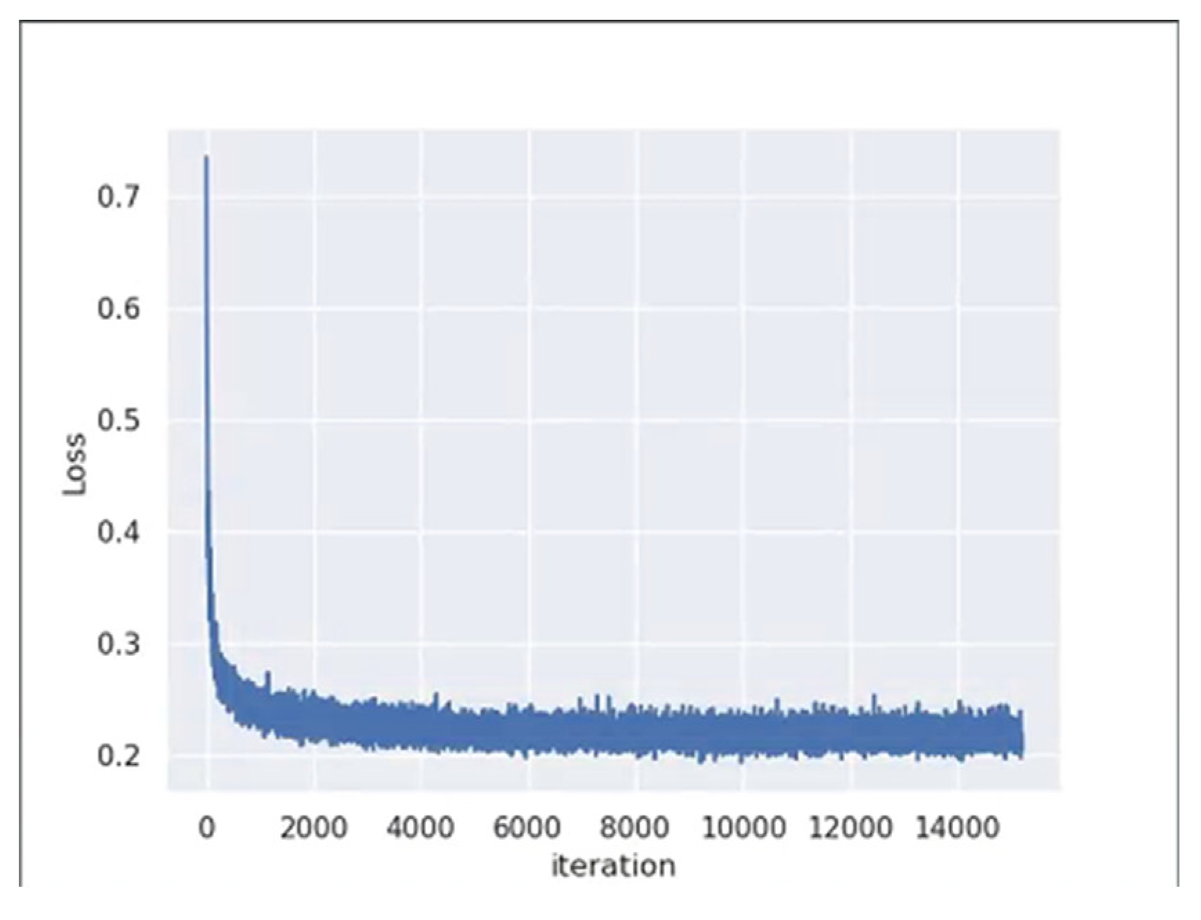
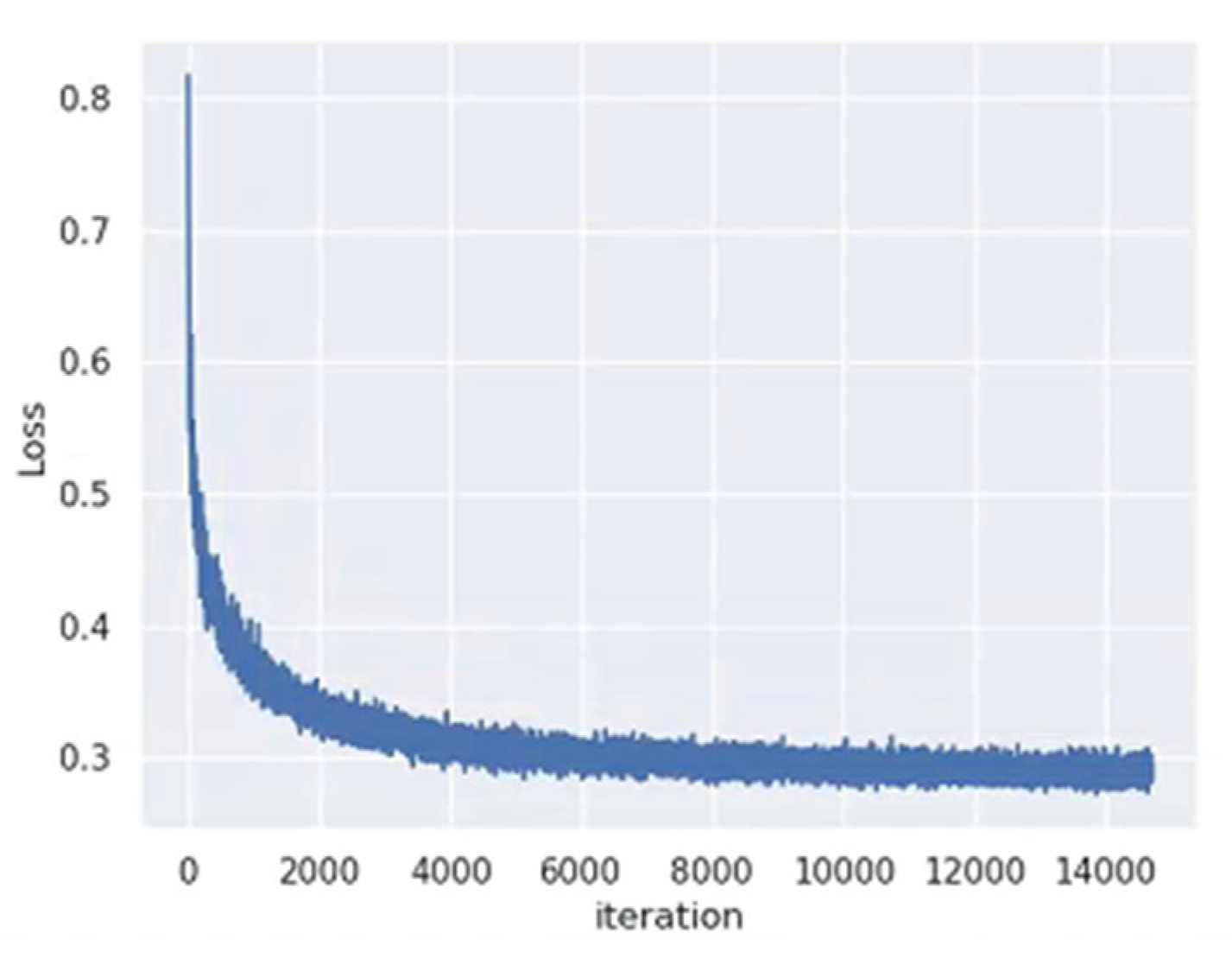
To assess the validity of HPSH, we compared it with different hash methods, including KSLSH [9], MiLan [34] with Hamming distance, MiLan with Euclidean distance, MiLan with hard probability sampling, and HPSH with hard probability sampling on the UCMD dataset. Figure 6 shows the result of the top 20 retrieved images using our HPSH method for four query images. Figure 7 depicts the loss during training. These results show that the loss drops quickly before the first 2000 iterations, after which it stabilizes.
Table 3 shows mAP@20 and retrieval time results of KSLSH [9], MiLan [33] with Hamming distance, MiLan [33] with Euclidean distance, HPSH, HPSH+S with Hamming distance, and HPSH+S with Euclidean distance on the UCMD dataset with different hash bits. It is worth pointing out that for the results of the MiLan approach, “MiLan” means that the original framework was adopted with semi-hard sampling; “MiLan+S” means that semi-hard sampling is replaced by the proposed hard probability sampling.
The results in Table 3 illustrate that our HPSH+S produces state-of-the-art hash retrieval results on the UCMD dataset. Specifically, compared with KSLSH, we achieve significant improvements. When the number of hash bits is 16, 24, and 32, the improvements are 35% (from 55.7% to 90.9%), 33% (from 59.4% to 92.2%), and 30% (from 63% to 92.8%), respectively. All of the results of HPSH+S are better than those of the existing state-of-art hash method. When compared with MiLan, the results are increased by 3.4% (from 87.5% to 90.9%), 3.2% (from 89.0% to 92.2%), and 2.4% (from 90.4% to 92.8%), respectively. We can see from the results that sampling can greatly improve the retrieval performance. For HPSH, the performance is improved from 0.815 to 0.909 for 16 bits; from 0.841 to 0.922 for 24 bits; and from 0.850 to 0.928 for 32 bits. Moreover, it can also be proved that the proposed hard probability mining method works well not only in the HPSH framework but also in the MiLan [33] framework. If we substitute the semi-hard mining strategy in MiLan [33] with the proposed hard probability sampling strategy, the performance is improved from 0.875 to 0.904 for 16 bits; from 0.890 to 0.911 for 24 bits; and from 0.904 to 0.918 for 32 bits.
We can see from Table 3 that as the hash codes lengthen, mAP@20 becomes better. We can see that when L = 16 bits, the results of retrieval are the worst, and dimensional reduction has a serious impact on the results. When the number of hash bits is 24 and 32, the mAP@20 values improve. Therefore, for the hashing method, shorter lengths of hash codes cause the performance to drop. However, when the hash code becomes longer, the impact becomes smaller. From the HPSH+S, HPSH+S (Euclidean), MiLan [33], and MiLan [33] (Euclidean) results listed in Table 3, we can observe the degradation of retrieval performance due to binarization. For MiLan [33], when the number of hash bits is 16, 24, and 32, the results are reduced by 2.8% (from 90.3% to 87.5%), 0.4% (from 89.4% to 89.0%), and 1.2% (from 91.6% to 90.4%). For HPSH+S, when the number of hash bits is 16, 24, and 32, the results are reduced by 1.4% (from 92.3% to 90.9%), 0.7% (from 92.9% to 92.2%), and 0.2% (from 93.0% to 92.8%). We find that our HPSH+S method results in less of a decline because of binarization compared with MiLan. This benefit is the result of our two hash loss functions. Binary hash codes can save a lot of retrieval time. For MiLan, when the number of hash bits is 16, 24, and 32, the time saved is 10 ms (from 35.3 ms to 25.3 ms), 10.3 ms (from 35.8 ms to 25.5 ms), and 10.4 ms (from 36.0 ms to 25.6 ms). At the same time, the needed space to store binary codes is much less, and as the length of data increases, this decrease becomes more pronounced.
The improvement demonstrates that our hard sample method can select more informative and stable samples to produce better retrieval results. It is noteworthy that the results of the HPSH+S method with Hamming distance are even better than the results of Euclidean distance with MiLan. We observe improvements of 0.6% (from 90.3% to 90.9%), 2.8% (from 89.4% to 92.2%), and 1.2% (from 91.6% to 92.8%), respectively. In order to complete the control trial, we also analyzed the results calculated by Euclidean distance; obviously, the results are better.
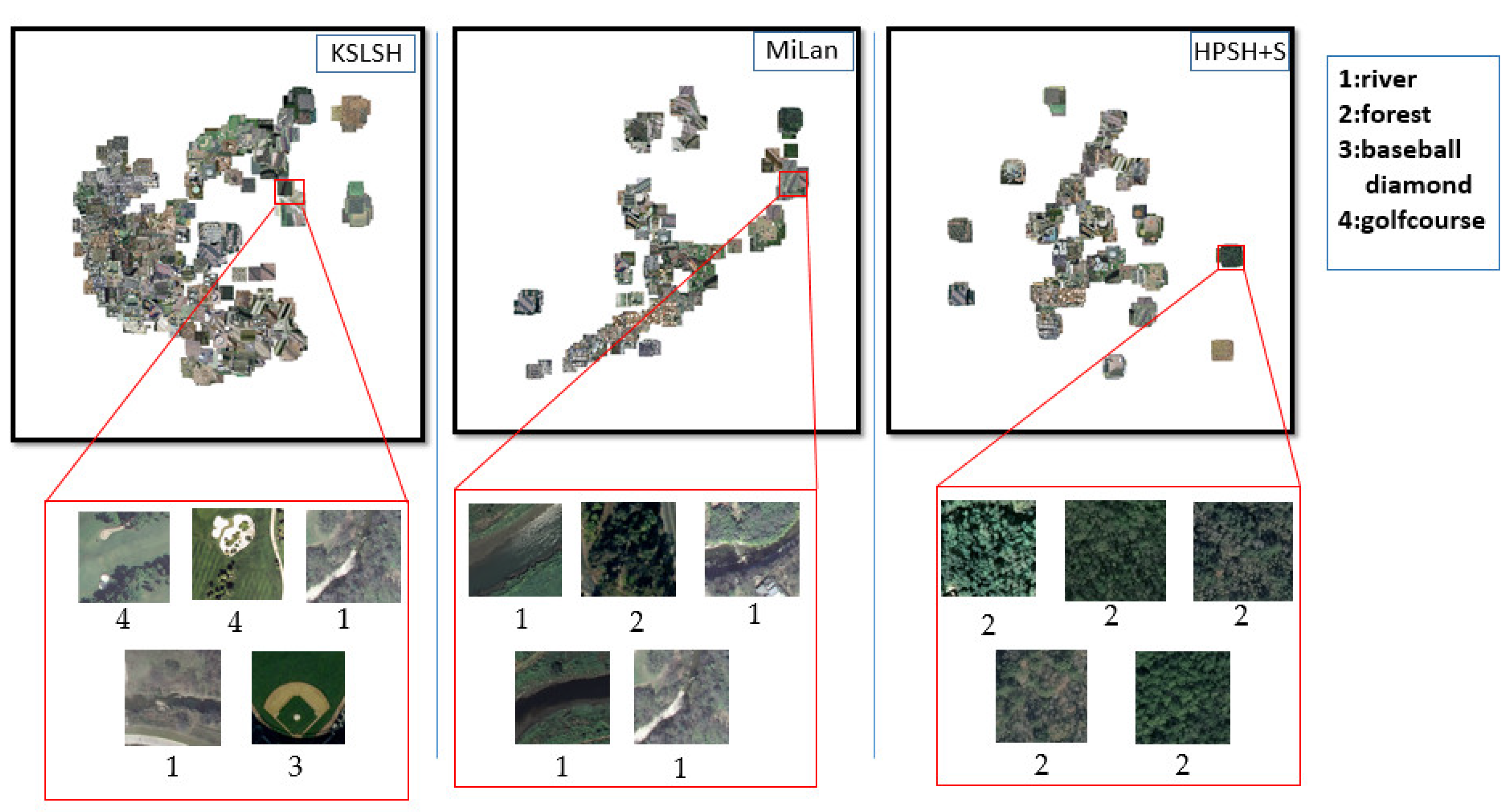
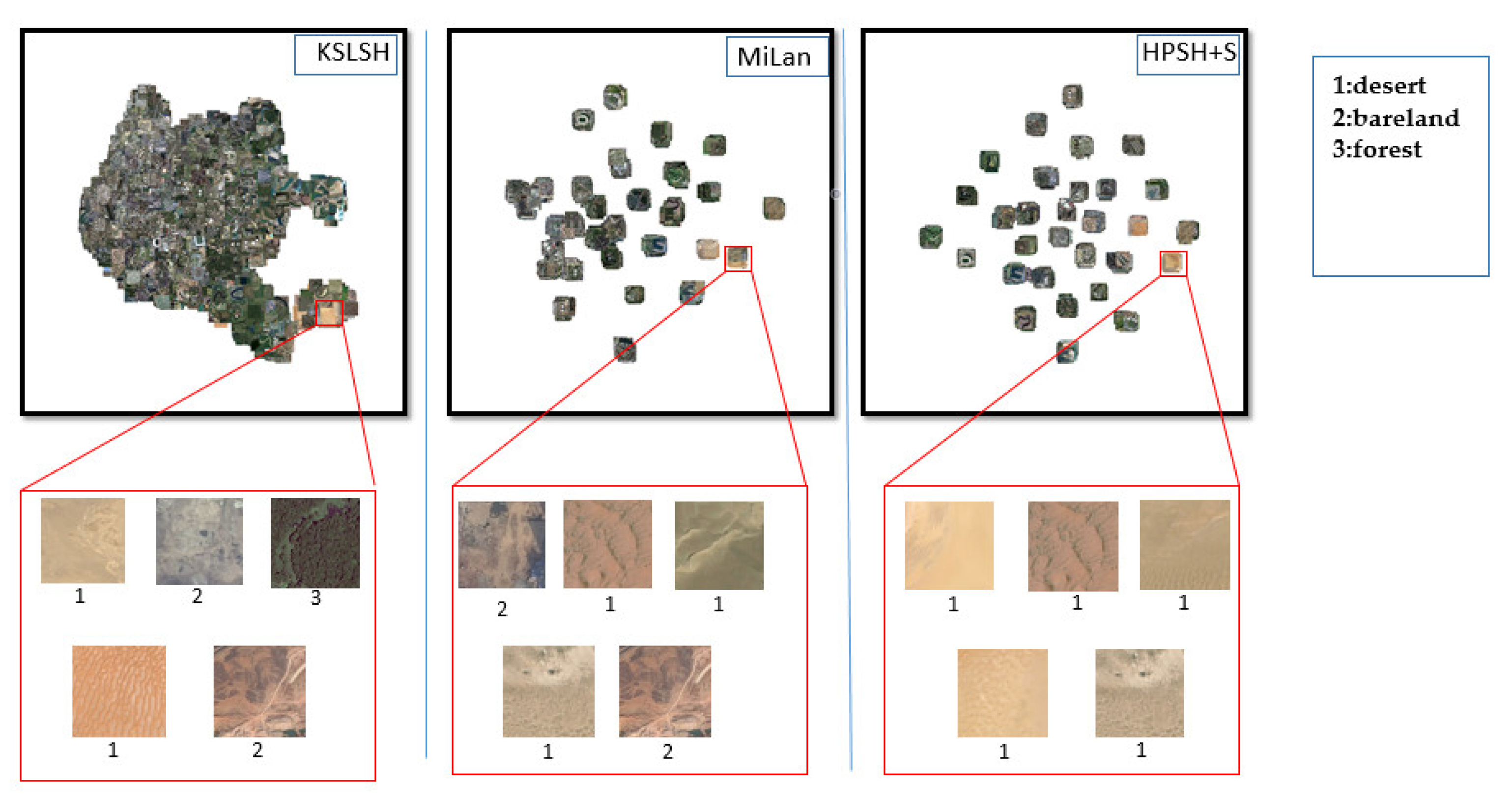
We report the t-distributed stochastic neighbor embedding (t-SNE) results in Figure 8. We can see that our HPSH method produces the best distinguishing effect, and the aggregation of similar samples is better. The improved hash retrieval results on the dataset of UCMD [10] indicate that HPSH is more effective than and superior to other excellent hash retrieval methods.
4.3.2. Results on Enhanced UCMD
We also report experimental results on UCMD with an enhanced dataset. We exploited data augmentation as in DHNN [5]. Specifically, each image in the UCMD dataset was rotated by 90, 180, and 270 degrees, which resulted in an augmented UCMD dataset with 8400 images. Then, we selected 7400 images at random for training, and the remaining 1000 images were chosen for evaluation. Table 4 compares the HPSH+S method with DPSH, DHNN, and MiLan. As Table 4 shows, our HPSH improves the mAP@20 with 32 bits from DPSH (74.8%), DHNN (93.9%), and MiLan (97.7%) to 99.6%, and with 64 hash bits, the proposed HPSH method improves the mAP from DPSH (81.7%), DHNN (97.1%), and MiLan (99.1%) to 99.7%. These results prove that the HPSH method is able to produce better results when hash bits are small, and the volume of the training set affects the performance.
4.3.3. Results on AID
In experiments on the AID dataset, we used 60% of samples from each class for training and the remaining 40% for testing. The results on AID show the same tendency as those on UCMD.
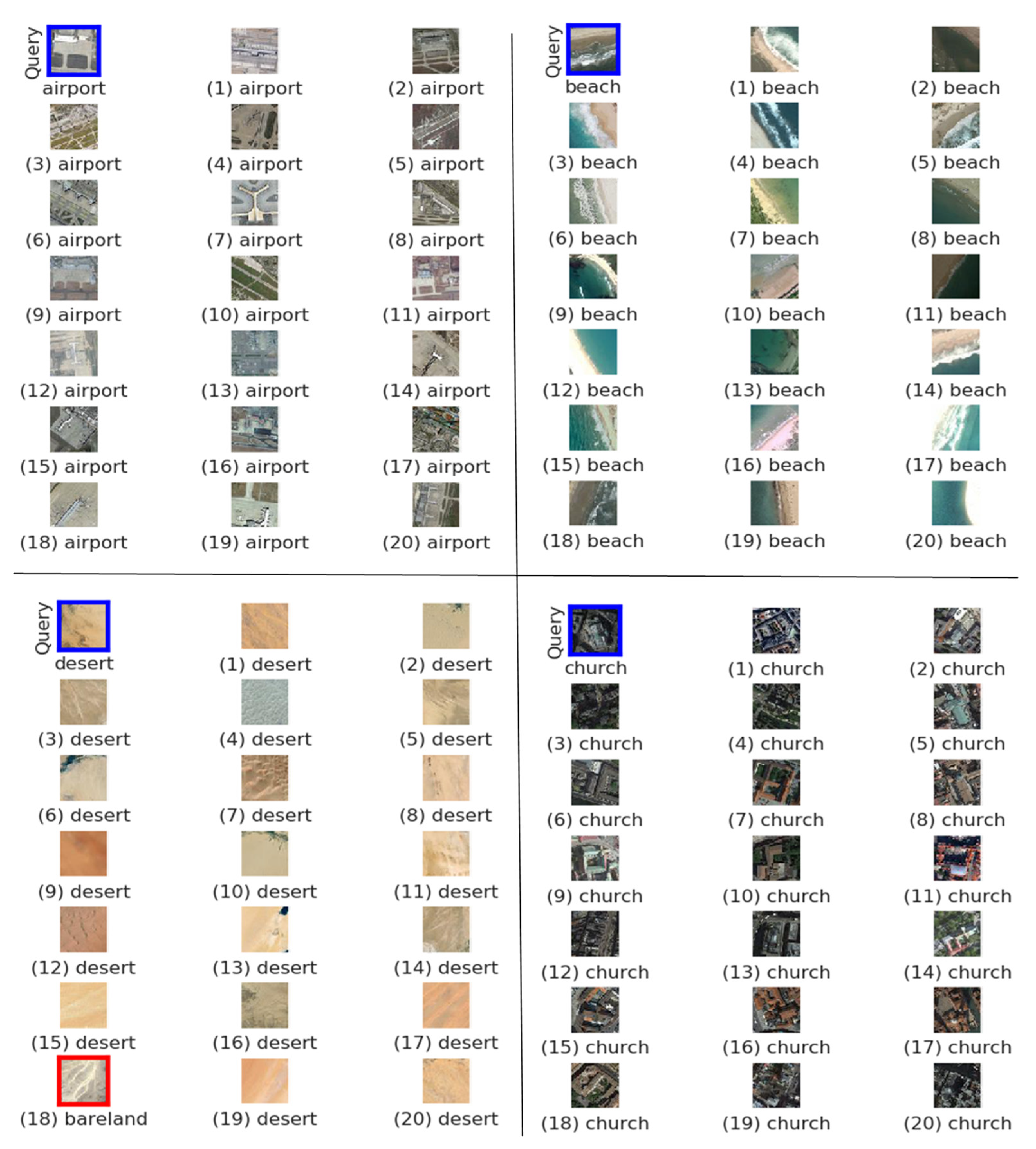
We show the results of the top 20 retrieved images for query images from four different classes, namely, airport, beach, desert, and church, in Figure 9. Figure 10 depicts the loss trend during training.
Table 5 shows the results of KSLSH [9], MiLan [33] with Hamming distance, MiLan [33] with Euclidean distance, MiLan+S, HPSH, HPSH+S with Hamming distance, and HPSH+S with Euclidean distance on the AID dataset with different hash bits. We mainly list the mAP@20 values to demonstrate the validity of our HPSH on the AID dataset. The results prove that our HPSH exceeds the retrieval results of state-of-the-art hash methods on the AID dataset.
Specifically, compared with KSLSH, our HPSH+S achieves significant improvements when the number of hash bits is 16, 24, and 32 with improvements of 46% (from 42.6% to 89.8%), 47% (from 46.7% to 93.6%), and 44% (from 49.5% to 94.2%), respectively. We can see that all of our proposed methods are better than the existing best method (MiLan): the results improve by 2.2% (from 87.6% to 89.8%), 4.5% (from 89.1% to 93.6%), and 1.6% (from 92.6% to 94.2%), respectively. These results prove that sampling can greatly improve the retrieval performance. For HPSH, the performance is improved from 0.723 to 0.898 for 16 bits; from 0.767 to 0.936 for 24 bits; and from 0.807 to 0.942 for 32 bits. Moreover, it can also be proved that the proposed hard probability sampling method works well not only in the HPSH framework but also in the MiLan framework. If we substitute the semi-hard mining strategy in MiLan with the proposed hard probability sampling strategy, the performance improves from 0.876 to 0.914 for 16 bits; from 0.891 to 0.930 for 24 bits; and from 0.926 to 0.946 for 32 bits. Since the MiLan+S method and HPSH+S only change the sampling method compared with the MiLan and HPSH, the improvement of our retrieval results confirms that our hard sampling method is effective, we can obtain more useful samples for training, and at the same time, random sampling will worsen the retrieval results to some extent on the AID dataset. Notably, our hard sampling method has a greater promoting effect on the AID dataset than on UCMD. The improvement demonstrates that our hard probability sampling can obtain more informative and stable samples to produce better retrieval results on AID. As for time consumption, we can see that we did not need extra time to improve retrieval precision. Clearly, our HPSH+S works well not only on the UCMD dataset but also on the AID dataset. We also provide the t-SNE results of AID in Figure 11. KSLSH [9] gets the worst discriminate t-SNE results. MiLan [33] and HPSH obtained better clustering results on AID. However, the best results came from our HPSH.
4.4. Ablation Study
In this section, we report the results of an ablation study conducted on a remote sensing dataset, and we analyze the hyper-parameters of the HPSH loss. Comparative results of different hash bits, different top K, and different training/testing ratios are listed. We also change the main metric learning loss to illustrate the margin loss’s effectiveness. The experimental results are presented in tabular form. In Table 6, we report the results of different mAP@K values when hash codes vary from 8 bits to 40 bits on the UCMD dataset. Table 7 shows the results of different hash code lengths with different training/testing ratios on the UCMD dataset. Clearly, the higher the proportion of training data, the better the retrieval result. We also change our metric learning loss and present the results of a contrastive loss and triplet loss in Table 8.
We performed experiments by fixing the most appropriate two parameters, α and β of Equation (5), on the UCMD dataset. The first step was to fix the value of α at 0.3, and the value of β was varied from 0.0 to 1.0. Table 9 lists mAP@20 values, which show that the best results are obtained with β value of 0.6. The second step was to fix the value of β at 0.6. We changed α from 0.0 to 1.0. Table 10 shows mAP@20 values, which shows that the best results are obtained with a β value of 0.6. Therefore, the values of α and β are set to 0.6 and 0.3, respectively.
4.5. Discussion
Overall, when considering these methods of hash image retrieval, our loss gains a novel result and achieves state-of-the-art performance on UCMD and AID. Moreover, we find that longer hash codes work better. This reveals that feature representation with a relatively high dimension will yield a more discriminative performance. However, by using the binarization of low dimensional features, we greatly reduce the occupied storage space and the retrieval time. Moreover, our HPSH could also obtain excellent and competitive results with hard probability sampling when compared with the baselines. The results verify the validity of our HPSH.
5. Conclusions
A new hash retrieval method named HPSH is proposed in this paper, which makes full use of a sample selection strategy to acquire informative training samples and a hash margin loss to carry out hash code learning in RSIR. First, we established a hard negative probability sampling method that picks more scattered samples to train the network: this is the key to improving retrieval performance. Second, we designed a novel hash loss function with three components, and a margin loss is used to calculate feature similarity; the hash-like loss function is used to make hash-like codes more similar to hash codes; a hash code balance loss is used to balance the 0 and 1 in hash codes. The final loss function can better train the network parameters while reducing the hashing accuracy loss due to quantization. Finally, the HPSH method achieves superior results to those of other state-of-the-art hash image retrieval methods. For the UCMD dataset, our HPSH+S obtained a mAP@20 of up to 90.9% on 16 hash bits, 92.2% on 24 hash bits, and 92.8% on 32 hash bits. For the AID dataset, our HPSH+S obtained a mAP@20 value of 89.8% on 16 hash bits, 93.6% on 24 hash bits, and 95.5% on 32 hash bits. For the UCMD dataset with data augmentation, our HPSH obtained a mAP@20 value of 99.6% on 32 hash bits and 99.7% on 64 hash bits. In the future, we will consider designing a more advanced deep hash network in which the hash code carries more accurate information, and we will also verify the scalability of our work on other retrieval tasks.
Author Contributions
P.L. designed the research topic, modified the improper expression of the article, and guided work process. X.S. conducted experimental verification of the deep hard probability sampling hash retrieval method, finished the paper and corrected it for final publication. G.G., Z.W., and Q.Z. revised the paper and verify experimental results. All authors have read and agreed to the published version of the manuscript.
Funding
This research was funded by the Nature Science Foundation of China, under Grants 61841602, the fundamental Research Funds of Central Universities, JLU, General Financial Grant from China Postdoctoral Science Foundation, under Grants 2015M571363 and 2015M570272,the Provincial Science and Technology Innovation Special Fund Project of Jilin Province, under Grant 20190302026GX, the Jilin Province Development and Reform Commission Industrial Technology Research and Development Project, under Grant 2019C054-4, and the State Key Laboratory of Applied Optics Open Fund Project, under Grant20173660. Jilin Provincial Natural Science Foundation No.20200201283JC. Foundation of Jilin Educational Committee No. JJKH20200994KJ.
Conflicts of Interest
The authors declare no conflict of interest.
References
- Ma, Y.; Wu, H.; Wang, L.; Huang, B.; Ranjan, R.; Zomaya, A.; Jie, W. Remote sensing big data computing: Challenges and opportunities. Future Gener. Comput. Syst. 2015, 51, 47–60. [Google Scholar] [CrossRef]
- Mandal, D.; Annadani, Y.; Biswas, S. GrowBit: Incremental Hashing for Cross-Modal Retrieval. In Asian Conference on Computer Vision; Springer: Cham, Switzerland, 2018; pp. 305–321. [Google Scholar]
- Tong, X.-Y.; Xia, G.-S.; Hu, F.; Zhong, Y.; Datcu, M.; Zhang, L. Exploiting Deep Features for Remote Sensing Image Retrieval: A Systematic Investigation. IEEE Trans. Big Data 2019, 6. [Google Scholar] [CrossRef] [Green Version]
- Zhao, L.; Tang, J.; Yu, X.; Li, Y.; Mi, S.; Zhang, C. Content-Based Remote Sensing Image Retrieval Using Image Multi-feature Combination and SVM-Based Relevance Feedback. In Recent Advances in Computer Science and Information Engineering: Volume 1; Qian, Z., Cao, L., Su, W., Wang, T., Yang, H., Eds.; Springer: Berlin, Germany, 2012; pp. 761–767. [Google Scholar] [CrossRef]
- Daschiel, H.; Datcu, M. Information mining in remote sensing image archives: System evaluation. IEEE Trans. Geosci. Remote. Sens. 2005, 43, 188–199. [Google Scholar] [CrossRef]
- Schroff, F.; Kalenichenko, D.; Philbin, J. FaceNet: A Unified Embedding for Face Recognition and Clustering. arXiv 2015, arXiv:1503.03832. [Google Scholar]
- Szegedy, C.; Vanhoucke, V.; Ioffe, S.; Shlens, J.; Wojna, Z. Rethinking the Inception Architecture for Computer Vision. arXiv 2015, arXiv:1512.00567. [Google Scholar]
- Li, W.-J.; Wang, S.; Kang, W.-C. Feature Learning based Deep Supervised Hashing with Pairwise Labels. arXiv 2015, arXiv:1511.03855. [Google Scholar]
- Demir, B.; Bruzzone, L. Hashing-Based Scalable Remote Sensing Image Search and Retrieval in Large Archives. IEEE Trans. Geosci. Remote. Sens. 2015, 54, 892–904. [Google Scholar] [CrossRef]
- Dai, O.E.; Demir, B.; Sankur, B.; Bruzzone, L. A Novel System for Content-Based Retrieval of Single and Multi-Label High-Dimensional Remote Sensing Images. IEEE J. Sel. Top. Appl. Earth Obs. Remote. Sens. 2018, 11, 2473–2490. [Google Scholar] [CrossRef] [Green Version]
- Xia, G.-S.; Hu, J.; Hu, F.; Shi, B.; Bai, X.; Zhong, Y.; Zhang, L.; Lu, X. AID: A Benchmark Data Set for Performance Evaluation of Aerial Scene Classification. IEEE Trans. Geosci. Remote. Sens. 2017, 55, 3965–3981. [Google Scholar] [CrossRef] [Green Version]
- Lowe, D.G. Similarity Metric Learning for a Variable-Kernel Classifier. Neural Comput. 1995, 7, 72–85. [Google Scholar] [CrossRef]
- Mika, S.; Ratsch, G.; Weston, J.; Scholkopf, B.; Mullers, K.R. Fisher Discriminant Analysis with Kernels. In Proceedings of the 1999 IEEE Signal Processing Society Workshop: Neural Networks for Signal Processing IX, Madison, WI, USA, 23–25 August 1999. [Google Scholar]
- Xing, E.P.; Ng, A.Y.; Jordan, M.I.; Russell, S.J. Distance Metric Learning with Application to Clustering with Side-Information. In Proceedings of the International Conference on Neural Information Processing Systems, Vancouver, BC, Canada, 9–14 December 2002. [Google Scholar]
- Hadsell, R.; Chopra, S.; Lecun, Y. Dimensionality reduction by learning an invariant mapping. In Proceedings of the 2006 IEEE Computer Society Conference on Computer Vision and Pattern Recognition (CVPR’06), New York, NY, USA, 17–22 June 2006. [Google Scholar]
- Hoffer, E.; Ailon, N. Deep metric learning using Triplet network. arXiv 2014, arXiv:1412.6622. [Google Scholar]
- Song, H.O.; Xiang, Y.; Jegelka, S.; Savarese, S. Deep Metric Learning via Lifted Structured Feature Embedding. arXiv 2015, arXiv:1511.06452. [Google Scholar]
- Wang, X.; Hua, Y.; Kodirov, E.; Robertson, N.M. Ranked List Loss for Deep Metric Learning. arXiv 2019, arXiv:1903.03238. [Google Scholar]
- Wu, C.-Y.; Manmatha, R.; Smola, A.J.; Krähenbühl, P. Sampling Matters in Deep Embedding Learning. arXiv 2017, arXiv:1706.07567. [Google Scholar]
- Bell, S.; Bala, K. Learning visual similarity for product design with convolutional neural networks. ACM Trans. Graph. 2015, 34, 1–10. [Google Scholar] [CrossRef]
- Chopra, S.; Hadsell, R.; Lecun, Y. Learning a similarity metric discriminatively, with application to face verification. In Proceedings of the 2005 IEEE Computer Society Conference on Computer Vision and Pattern Recognition (CVPR’05), San Diego, CA, USA, 20–25 June 2005. [Google Scholar]
- Parkhi, O.M.; Vedaldi, A.; Zisserman, A. Deep Face Recognition. In Proceedings of the British Machine Vision Conference 2015, Swansea, UK, 7–10 September 2015. [Google Scholar]
- Simo-Serra, E.; Trulls, E.; Ferraz, L.; Kokkinos, I.; Fua, P.; Moreno-Noguer, F. Discriminative Learning of Deep Convolutional Feature Point Descriptors. In Proceedings of the 2015 IEEE International Conference on Computer Vision (ICCV), Santiago, Chile, 7–13 December 2015; pp. 118–126. [Google Scholar]
- Zhao, P.; Zhang, T. Stochastic Optimization with Importance Sampling for Regularized Loss Minimization. In Proceedings of the 32nd International Conference on Machine Learning (ICML), Lillc, France, 7–9 July 2015; Volume 37, pp. 1–9. [Google Scholar]
- David, G.B.C. Distinctive Image Features from Scale-Invariant Keypoints. Int. J. Comput. Vis. 2004, 60, 91–110. [Google Scholar] [CrossRef]
- Oliva, A.; Torralba, A. Modeling the Shape of the Scene: A Holistic Representation of the Spatial Envelope. Int. J. Comput. Vis. 2001, 42, 145–175. [Google Scholar] [CrossRef]
- Babenko, A.; Slesarev, A.; Chigorin, A.; Lempitsky, V.S.J.A. Neural Codes for Image Retrieval. arXiv 2014, arXiv:1404.1777. [Google Scholar]
- Krizhevsky, A.; Hinton, G.E. Using very deep autoencoders for content-based image retrieval. In Proceedings of the 19th European Symposium on Artificial Neural Networks (ESANN), Bruges, Belgium, 27–29 April 2011. [Google Scholar]
- Krizhevsky, A.; Sutskever, I.; Hinton, G. ImageNet Classification with Deep Convolutional Neural Networks. In Proceedings of the Neural Information Processing Systems Conference (NIPS), Lake Tahoe, NV, USA, 3–8 December 2012. [Google Scholar]
- Salakhutdinov, R.; Hinton, G. Semantic hashing. Int. J. Approx. Reason. 2009, 50, 969–978. [Google Scholar] [CrossRef] [Green Version]
- Li, Y.-S.; Zhang, Y.; Huang, X.; Zhu, H.; Ma, J. Large-Scale Remote Sensing Image Retrieval by Deep Hashing Neural Networks. IEEE Trans. Geosci. Remote. Sens. 2018, 56, 950–965. [Google Scholar] [CrossRef]
- Li, Y.-S.; Zhang, Y.; Huang, X.; Ma, J. Learning Source-Invariant Deep Hashing Convolutional Neural Networks for Cross-Source Remote Sensing Image Retrieval. IEEE Trans. Geosci. Remote. Sens. 2018, 56, 6521–6536. [Google Scholar] [CrossRef]
- Roy, S.; Sangineto, E.; Demir, B.; Sebe, N. Deep Metric and Hash-Code Learning for Content-Based Retrieval of Remote Sensing Images. In Proceedings of the2018 IEEE International Geoscience and Remote Sensing Symposium (IGARSS 2018), Valencia, Spain, 22–27 July 2018; pp. 4539–4542. [Google Scholar] [CrossRef] [Green Version]
- Chen, Y.; Lu, X. A Deep Hashing Technique for Remote Sensing Image-Sound Retrieval. Remote Sens. 2019, 12, 84. [Google Scholar] [CrossRef] [Green Version]
- Kulis, B.; Grauman, K. Kernelized Locality-Sensitive Hashing for Scalable Image Search. In Proceedings of the International Conference on Computer Vision (ICCV), Kyoto, Japan, 27 September–4 October 2009; pp. 2130–2137. [Google Scholar] [CrossRef]
- Weiss, Y.; Torralba, A.; Fergus, R. Spectral Hashing. In Proceedings of the 22nd Annual Conference on Neural Information Processing Systems (NIPS’08), Vancouver, BC, Canada, 8–10 December 2008; Curran Associates Inc.: Red Hook, NY, USA, 2008; pp. 1753–1760. [Google Scholar]
- Liu, W.; Wang, J.; Ji, R.; Jiang, Y.-G.; Chang, S. Supervised Hashing with Kernels. In Proceedings of the 2012 IEEE Conference on Computer Vision and Pattern Recognition, Providence, RI, USA, 16–21 June 2012. [Google Scholar] [CrossRef]
- Al Lehnen; Gary E Wesenberg; The Sphere Game in n Dimensions. Available online: http://faculty.madisoncollege.edu/alehnen/sphere/hypers.htm (accessed on 3 May 2002).
- Gong, Y.; Lazebnik, S.; Gordo, A.; Perronnin, F. Iterative Quantization: A Procrustean Approach to Learning Binary Codes for Large-Scale Image Retrieval. IEEE Trans. Pattern Anal. Mach. Intell. 2012, 35, 2916–2929. [Google Scholar] [CrossRef] [PubMed] [Green Version]
- Hyvrinen, A.; Hurri, J.; Hoyer, P.O. Natural Image Statistics: A Probabilistic Approach to Early Computational Vision; Springer Publishing Company, Inc.: Berlin, Germany, 2009. [Google Scholar]
- Maas, A.L.; Hannun, A.Y.; Ng, A.Y. Rectifier nonlinearities improve neural network acoustic models. In Proceedings of the ICML Workshop on Deep Learning for Audio, Speech and Language, Atlanta, GA, USA, 16 June 2013. [Google Scholar]
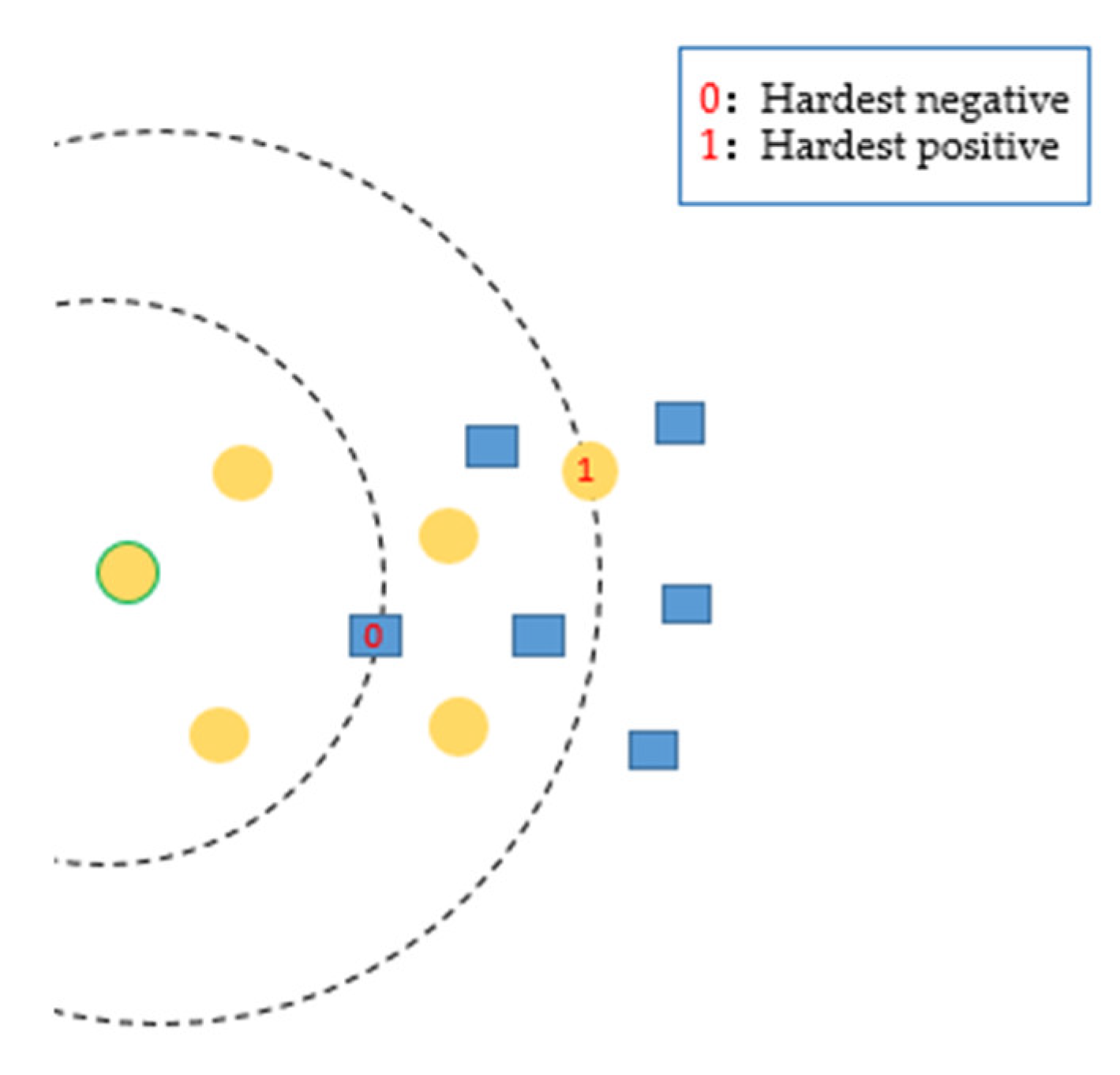
Figure 1.
Different colors represent different categories: the centered yellow point is the anchor. The yellow point with the red “1” is the positive sample farthest from the anchor, which represents the hardest positive sample. Then, blue with the red “0” is the closest negative sample to the anchor. We draw two semicircles on the basis of these two points, and then all points inside the ring are informative samples because, in loss computation, they can provide more valuable information and make the training process converge quickly.

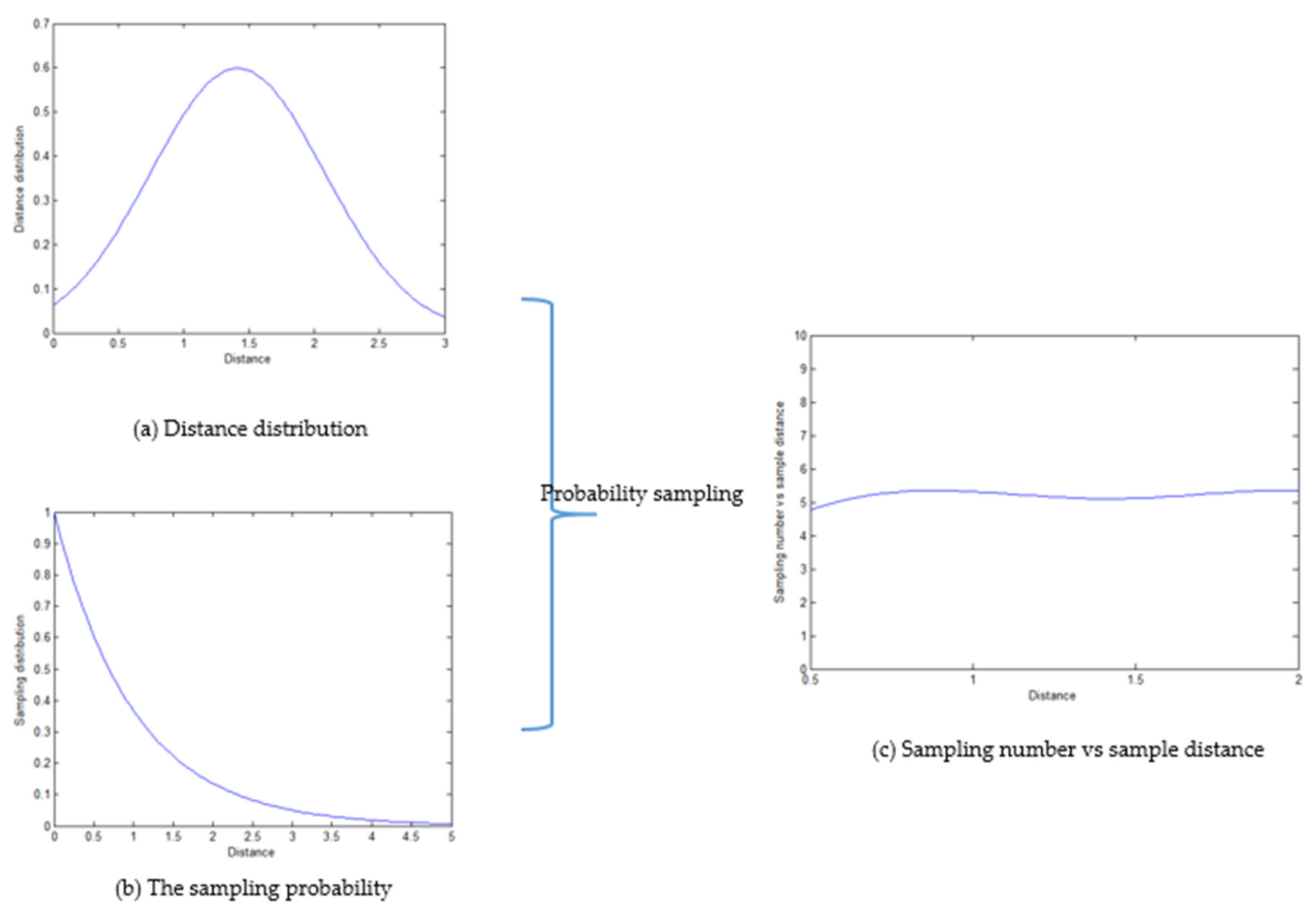
Figure 2.
(a) The distance distribution. (b) The sampling probability. (c) Sampling number vs. sample distance.
Figure 2.
(a) The distance distribution. (b) The sampling probability. (c) Sampling number vs. sample distance.

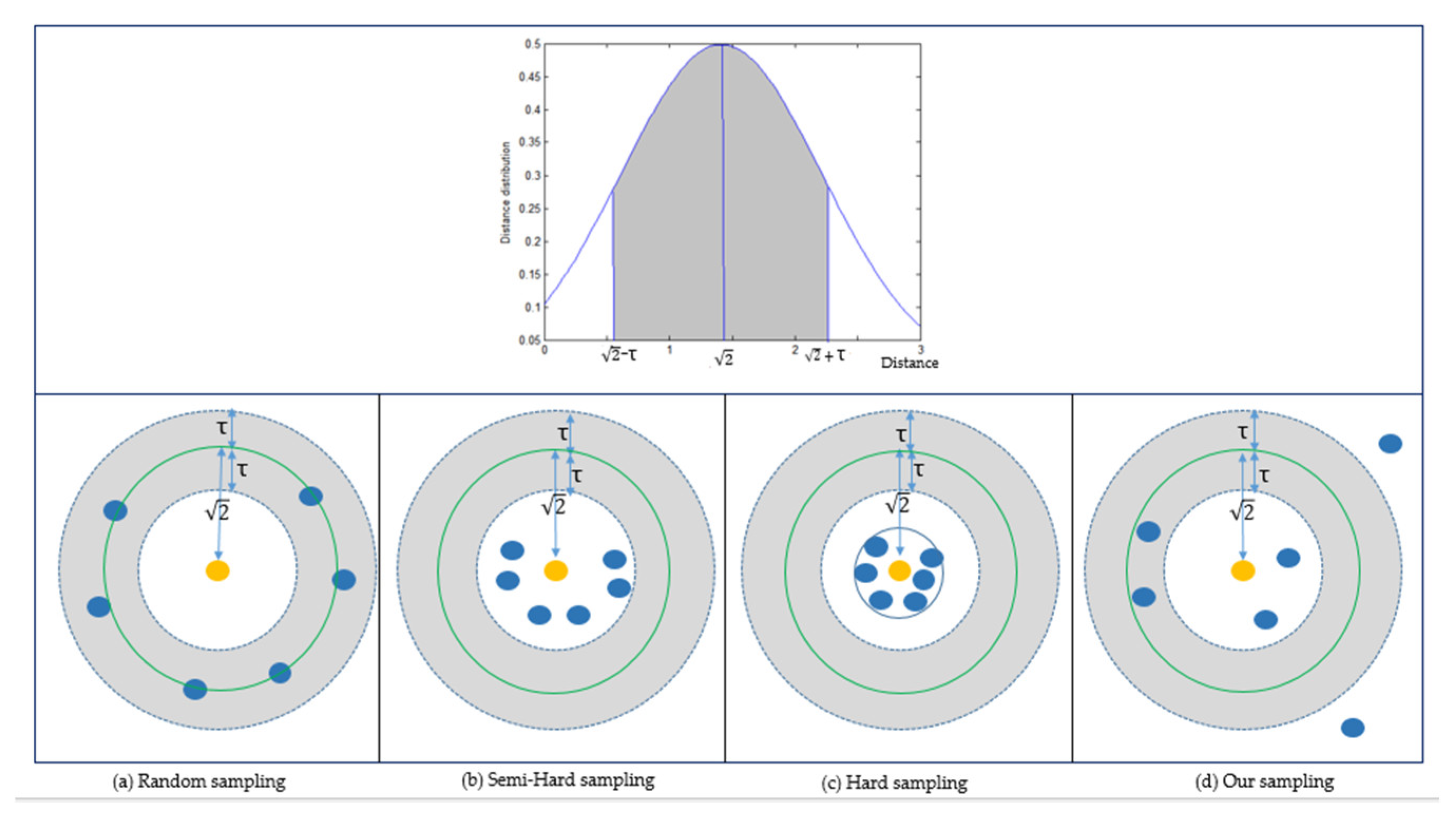
Figure 3.
Four sampling methods are shown in (a–d). The above figure shows the distribution probability density of sample distance. As the sample distance roughly follows a normal distribution (), we put the mean at , and is a randomly selected boundary to denote a centrally symmetrical distribution area (the shaded zone). In the subfigures below, the centered yellow point represents the anchor, and the blue points represent the negative samples selected by different sampling methods. In (a), most of the selected samples are gathered in the shaded zone around in random sampling. (b) represents semi-hard sampling. The selected samples need to be close to the anchor, but not as close as that needed in hard mining. (c) shows hard sampling. A predefined boundary (denoted by the blue circle) is used to filter hard negative samples. Thus, the selected samples are gathered more closely to the anchor than those in semi-hard sampling. (d) Our proposed sampling strategy. The selected samples have a scattered distribution to maintain diversity in the training batch.

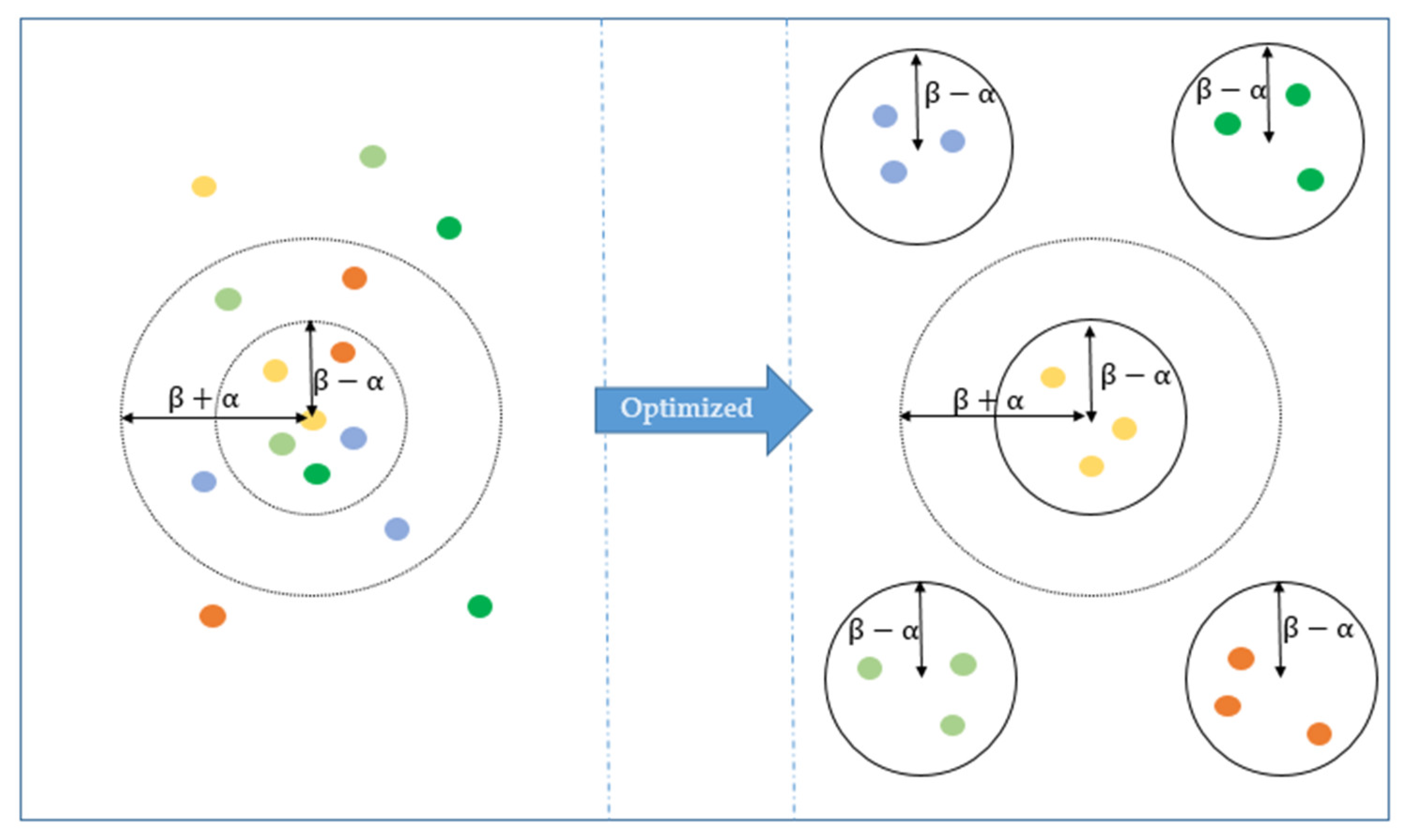
Figure 4.
The optimization process using the margin loss. The colored points represent samples belonging to different classes. The left shows the initial distribution. The right shows the final state after optimization. The black solid circle represents the boundary for each of class, which is used to restrict samples of the same category within a given distance. The black dotted circle is a different class boundary applied to separate different categories.

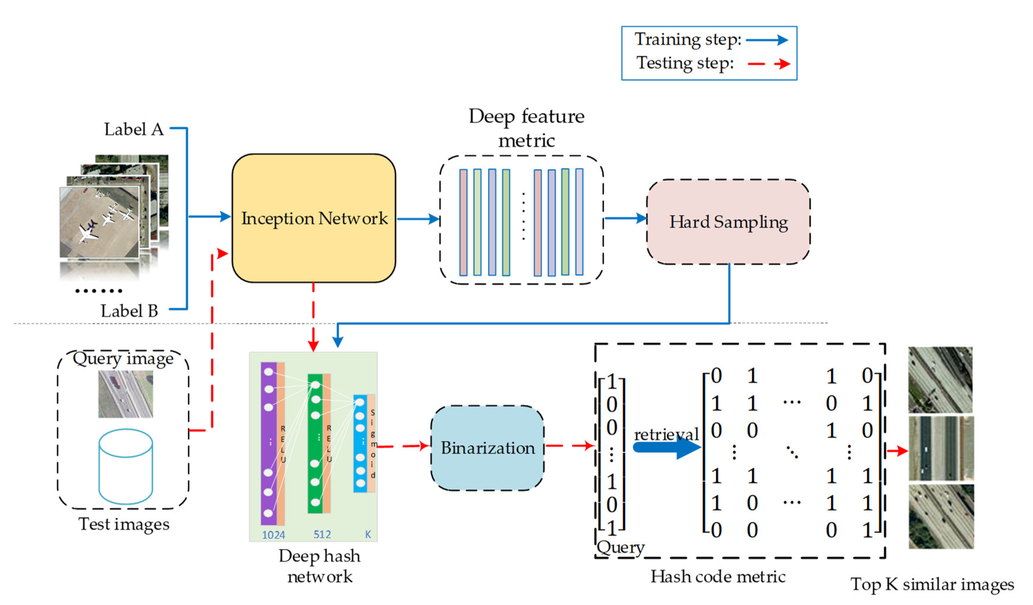
Figure 5.
The architecture of our HPSH with hard probability sampling (HPSH+S) method. It can be divided into four parts. First, we use Inception Net to extract deep embedding of the remote sensing dataset. Second, we obtain hard negative examples by a probability sampling method and create a training batch at the same time. Third, the training batch is sent to the deep hash network, which uses a deep neural network to obtain compacted hash-like codes. Finally, we calculate the loss function to backpropagate in the deep net. An additional binarization process was used in the testing process.

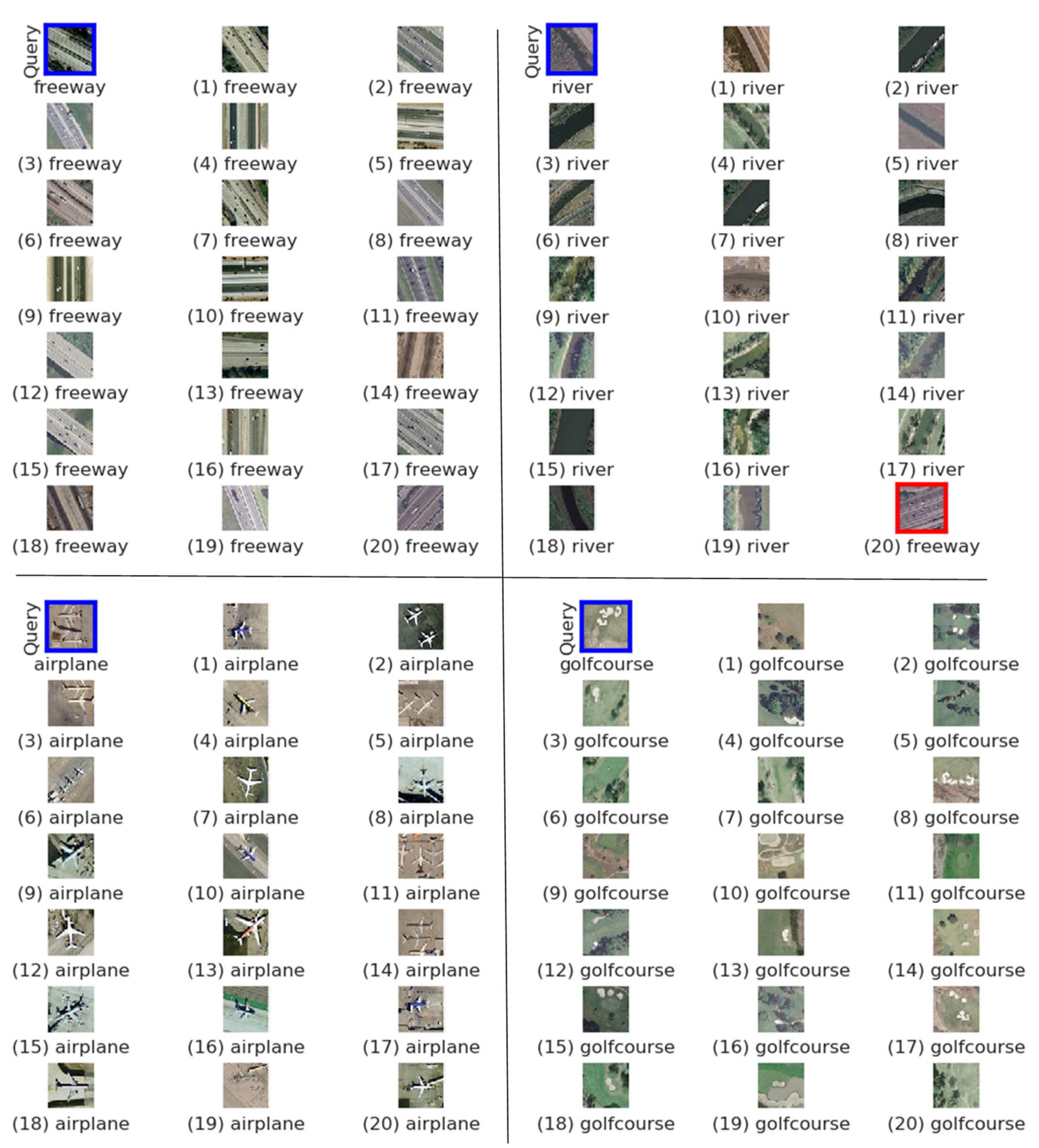
Figure 6.
The top 20 retrieval results of HPSH+S on the UCMD dataset. The black lines separate the search results for four images. The query image is bordered by the blue square. The wrong retrieved image is bordered by the red square. The words under the images represent the class to which the images belong.

Figure 7.
Trends in the loss change on the UCMD dataset.

Figure 8.
t-SNE 2D scatterplots comparing the 2D projection of the L-dimensional binary hash codes of the test images in the UCMD dataset. We map the tiny image in the small red box to the big red box, the number under the picture in the big red box represents the category label of the current picture, and the specific category is given in the blue box. The leftmost diagram is the t-SNE 2D scatterplot of KSLSH [9], the middle one is the t-SNE 2D scatterplot of MiLan, and the last one is the t-SNE 2D scatterplot of HPSH+S.

Figure 9.
The top 20 retrieval results of HPSH+S on the AID dataset. The black lines separate the search results for four images from four different categories. The query retrieval image is bordered by the blue square. The wrong retrieved image is bordered by the red square. The words under the picture represent the class to which the image belongs.

Figure 10.
Loss trend during training on the AID dataset.

Figure 11.
t-SNE 2D scatterplots comparing the 2D projection of the L-dimensional binary hash codes of the test images in the AID dataset. We map the tiny image in the small red box to the big red box. The number under the picture in the big red box represents the class label of the current image, and the specific class is given in the blue box. The leftmost diagram is the t-SNE 2D scatterplot of KSLSH, the middle one is the t-SNE 2D scatterplot of MiLan, and the last one is the t-SNE 2D scatterplot of HPSH+S.


Table 1.
Definition of some symbols.
| Symbol | Definition |
|---|---|
| X | The set of the remote sensing (RS) images |
| Y | The set of the labels |
| The m-th class j-th image | |
| The m-th class p-th image | |
| The l-th class n-th image | |
| The high dimensional embedding | |
| The low dimensional embedding | |
| The i-th hash-like code | |
| The i-th hash-code | |
| The Hamming distance |
Table 2.
The hash network structure. It consists of three fully connected (FC) layers and three activation functions. The first two layers are followed by LeakyRelu activation. The last layer is followed by Sigmoid activation.
Table 2.
The hash network structure. It consists of three fully connected (FC) layers and three activation functions. The first two layers are followed by LeakyRelu activation. The last layer is followed by Sigmoid activation.
| Layers | Input Dimension | Output Dimension | Filter Size | Stride |
|---|---|---|---|---|
| FC_1 | 2048 | 1024 | 1 | 1 |
| LeakyRelu | 1024 | 1024 | - | - |
| FC_2 | 1024 | 512 | 1 | 1 |
| LeakyRelu | 512 | 512 | - | - |
| FC_3 | 512 | L | 1 | 1 |
| Sigmoid | L | L | - | - |
Table 3.
mAP@20 and average time on the UCMD dataset.
| Methods | L = 16 Bits | L = 24 Bits | L = 32 Bits | |||
|---|---|---|---|---|---|---|
| map@20 | Time (ms) | map@20 | Time (ms) | map@20 | Time (ms) | |
| KSLSH [9] | 0.557 | 25.3 | 0.594 | 25.5 | 0.630 | 25.6 |
| MiLan [33] | 0.875 | 25.3 | 0.890 | 25.5 | 0.904 | 25.6 |
| MiLan (Euclidean) [33] | 0.903 | 35.3 | 0.894 | 35.8 | 0.916 | 36.0 |
| MiLan+S | 0.904 | 25.3 | 0.911 | 25.5 | 0.918 | 25.6 |
| HPSH | 0.815 | 25.3 | 0.841 | 25.5 | 0.850 | 25.6 |
| HPSH+S | 0.909 | 25.3 | 0.922 | 25.5 | 0.928 | 25.6 |
| HPSH+S (Euclidean) | 0.923 | 35.3 | 0.929 | 35.8 | 0.930 | 36.0 |
Table 4.
mAP@20 result with data augmentation for hash retrieval on the UCMD dataset.
| DPSH [8] | DHNN [31] | MiLan [33] | HPSH+S | |
|---|---|---|---|---|
| L = 32 bits | 0.748 | 0.939 | 0.977 | 0.996 |
| L = 64 bits | 0.817 | 0.971 | 0.991 | 0.997 |
Table 5.
mAP@20 and average time on the AID dataset.
| Methods | L = 16 Bits | L = 24 Bits | L = 32 Bits | |||
|---|---|---|---|---|---|---|
| map@20 | Time(ms) | map@20 | Time(ms) | map@20 | Time(ms) | |
| KSLSH [9] | 0.426 | 115.3 | 0.467 | 116.1 | 0.495 | 117.5 |
| MiLan [33] | 0.876 | 117.5 | 0.891 | 116.0 | 0.926 | 114.5 |
| MiLan+S | 0.914 | 117.5 | 0.930 | 116.0 | 0.946 | 114.5 |
| HPSH | 0.723 | 117.5 | 0.767 | 116.0 | 0.807 | 114.5 |
| HPSH+S | 0.898 | 117.5 | 0.936 | 116.0 | 0.955 | 114.5 |
Table 6.
Different mAP@K results when hash bits vary from 8 bits to 40 bits on the UCMD dataset with our HPSH+S method.
Table 6.
Different mAP@K results when hash bits vary from 8 bits to 40 bits on the UCMD dataset with our HPSH+S method.
| mAP@K | 8 Bits | 16 Bits | 24 Bits | 32 Bits | 40 Bits |
|---|---|---|---|---|---|
| mAP@10 | 67.08 | 90.92 | 92.63 | 92.87 | 92.55 |
| mAP@20 | 76.76 | 90.90 | 92.25 | 92.80 | 92.85 |
| mAP@40 | 81.88 | 88.22 | 90.95 | 92.32 | 90.71 |
Table 7.
Different mAP@20 results when hash bits vary from 8 bits to 40 bits and the training ratio varies from 0.4 to 0.8 on the UCMD dataset with our HPSH+S method.
Table 7.
Different mAP@20 results when hash bits vary from 8 bits to 40 bits and the training ratio varies from 0.4 to 0.8 on the UCMD dataset with our HPSH+S method.
| Train Test Ratio | 8 Bits | 16 Bits | 24 Bits | 32 Bits | 40 Bits |
|---|---|---|---|---|---|
| 4:6 | 70.87 | 88.41 | 89.62 | 90.61 | 90.87 |
| 5:5 | 71.71 | 89.30 | 91.22 | 91.45 | 91.83 |
| 6:4 | 76.82 | 90.91 | 92.25 | 92.80 | 92.88 |
| 7:3 | 79.88 | 91.92 | 93.22 | 93.25 | 93.69 |
| 8:2 | 82.82 | 92.74 | 93.28 | 93.29 | 93.89 |
Table 8.
Different mAP@20 results when using a different metric learning loss and hash bits vary from 8 bits to 40 bits on the UCMD dataset.
Table 8.
Different mAP@20 results when using a different metric learning loss and hash bits vary from 8 bits to 40 bits on the UCMD dataset.
| Loss Function | 8 Bits | 16 Bits | 24 Bits | 32 Bits | 40 Bits |
|---|---|---|---|---|---|
| Contrastive loss | 74.20 | 80.37 | 82.00 | 85.20 | 91.84 |
| Triplet loss | 37.20 | 81.22 | 85.40 | 89.23 | 90.26 |
| Margin loss | 76.76 | 90.90 | 92.25 | 92.80 | 92.85 |
Table 9.
Different mAP@20 results when hash bits vary from 8 bits to 40 bits and margin β varies from 0.0 to 1.0 on the UCMD dataset.
Table 9.
Different mAP@20 results when hash bits vary from 8 bits to 40 bits and margin β varies from 0.0 to 1.0 on the UCMD dataset.
| Margin-β | 8 Bits | 16 Bits | 24 Bits | 32 Bits | 40 Bits |
|---|---|---|---|---|---|
| 0.0 | 5.87 | 56.13 | 69.15 | 81.33 | 84.82 |
| 0.2 | 8.83 | 67.23 | 76.39 | 82.29 | 84.83 |
| 0.4 | 46.18 | 89.70 | 91.24 | 91.75 | 91.86 |
| 0.6 | 76.76 | 90.90 | 92.25 | 92.80 | 92.85 |
| 0.8 | 75.29 | 81.32 | 88.04 | 88.85 | 89.32 |
| 1.0 | 62.37 | 67.36 | 76.24 | 80.85 | 82.03 |
Table 10.
Different mAP@20 results when hash bits vary from 8 bits to 40 bits and margin α varies from 0.0 to 1.0 on the UCMD dataset.
Table 10.
Different mAP@20 results when hash bits vary from 8 bits to 40 bits and margin α varies from 0.0 to 1.0 on the UCMD dataset.
| Margin-α | 8 Bits | 16 Bits | 24 Bits | 32 Bits | 40 Bits |
|---|---|---|---|---|---|
| 0.0 | 65.04 | 76.61 | 77.00 | 77.64 | 79.08 |
| 0.1 | 69.01 | 85.52 | 87.00 | 87.25 | 89.57 |
| 0.2 | 69.55 | 87.89 | 90.16 | 90.38 | 91.21 |
| 0.3 | 76.76 | 90.90 | 92.25 | 92.80 | 92.85 |
| 0.4 | 72.27 | 86.83 | 90.28 | 90.52 | 91.15 |
| 0.5 | 71.57 | 85.21 | 87.41 | 89.52 | 89.88 |
© 2020 by the authors. Licensee MDPI, Basel, Switzerland. This article is an open access article distributed under the terms and conditions of the Creative Commons Attribution (CC BY) license (http://creativecommons.org/licenses/by/4.0/).
Share and Cite
MDPI and ACS Style
Shan, X.; Liu, P.; Gou, G.; Zhou, Q.; Wang, Z. Deep Hash Remote Sensing Image Retrieval with Hard Probability Sampling. Remote Sens. 2020, 12, 2789. https://0-doi-org.brum.beds.ac.uk/10.3390/rs12172789
AMA Style
Shan X, Liu P, Gou G, Zhou Q, Wang Z. Deep Hash Remote Sensing Image Retrieval with Hard Probability Sampling. Remote Sensing. 2020; 12(17):2789. https://0-doi-org.brum.beds.ac.uk/10.3390/rs12172789
Chicago/Turabian StyleShan, Xue, Pingping Liu, Guixia Gou, Qiuzhan Zhou, and Zhen Wang. 2020. "Deep Hash Remote Sensing Image Retrieval with Hard Probability Sampling" Remote Sensing 12, no. 17: 2789. https://0-doi-org.brum.beds.ac.uk/10.3390/rs12172789
Note that from the first issue of 2016, this journal uses article numbers instead of page numbers. See further details here.