Landsat-8 and Sentinel-2 Canopy Water Content Estimation in Croplands through Radiative Transfer Model Inversion


Department of Forest, Rangeland and Fire Sciences, College of Natural Resources, University of Idaho, Moscow, ID 83844, USA
*
Author to whom correspondence should be addressed.
Remote Sens. 2020, 12(17), 2803; https://0-doi-org.brum.beds.ac.uk/10.3390/rs12172803
Submission received: 29 July 2020
/
Revised: 27 August 2020
/
Accepted: 27 August 2020
/
Published: 29 August 2020
(This article belongs to the Special Issue Radiative Transfer Modelling in Remote Sensing Applications)
Abstract
:Despite the potential implications of a cropland canopy water content (CCWC) thematic product, no global remotely sensed CCWC product is currently generated. The successful launch of the Landsat-8 Operational Land Imager (OLI) in 2012, Sentinel-2A Multispectral Instrument (MSI) in 2015, followed by Sentinel-2B in 2017, make possible the opportunity for CCWC estimation at a spatial and temporal scale that can meet the demands of potential operational users. In this study, we designed and tested a novel radiative transfer model (RTM) inversion technique to combine multiple sources of a priori data in a look-up table (LUT) for inverting the NASA Harmonized Landsat Sentinel-2 (HLS) product for CCWC estimation. This study directly builds on previous research for testing the constraint of the leaf parameter (Ns) in PROSPECT, by applying those constraints in PRO4SAIL in an agricultural setting where the variability of canopy parameters are relatively minimal. In total, 225 independent leaf measurements were used to train the LUTs, and 102 field data points were collected over the 2015–2017 growing seasons for validating the inversions. The results confirm increasing a priori information and regularization yielded the best performance for CCWC estimation. Despite the relatively low variable canopy conditions, the inclusion of Ns constraints did not improve the LUT inversion. Finally, the inversion of Sentinel-2 data outperformed the inversion of Landsat-8 in the HLS product. The method demonstrated ability for HLS inversion for CCWC estimation, resulting in the first HLS-based CCWC product generated through RTM inversion.
1. Introduction
Agricultural drought, defined as the deficiency of soil moisture required for proper plant growth resulting in plant stress and yield reduction [1], is primarily monitored using agricultural drought indices [2]. Along with temperature, precipitation, and soil moisture content, vegetation (cropland) canopy water content (CCWC) is a known key parameter for monitoring agricultural drought due to its close relation to vegetation stress, biomass productivity, and nutrient transportation [3,4,5]. Although agricultural drought monitoring is important throughout the entire growing season [1], it is especially critical during growth periods where water shortages could result in significant loss of yield [6,7]. In irrigation-fed agricultural regions, CCWC is critical information for implementing flexible precision irrigation practices [4,8]. This is increasingly relevant, as growers seek to improve efficiency through the adoption of advanced irrigation technologies, which rely on precise, geographically distributed monitoring of water in- and out-flows from farm to basin scale [9]. The spaceborne remote sensing of CCWC eliminates the need for expensive, labor intensive field measurements, and minimizes uncertainties caused by within-field variations in soil type and microtopography [10,11]. Further development of remote sensing methods for CCWC assessment, is therefore of paramount importance.
Remote sensing techniques for the estimation of CCWC have been proposed relying on thermal, microwave, and optical data [4,12,13]. The detection of apparent thermal inertia through remote sensing by measuring surface albedo and the diurnal temperature range has been observed to have a proportional relationship with water content [14,15], although these methods perform poorly in heavily vegetated regions [16]. Microwave remote sensing methods for land surface water detection [17,18,19] show promising results for the detection of water content in agricultural drought monitoring applications [20,21], albeit lacking the combined temporal and spatial resolution required for operational agricultural applications [1]. The use of optical data relies primarily on the strong water absorption features in the 700–2500 nm spectral range. The increasing availability of moderate resolution (10–30 m) optical data, the development of data assimilation techniques for filling data gaps and decreasing space-borne product uncertainty [22,23], open the possibility of developing CCWC thematic products to meet the needs of operational users [24,25,26].
Optical-based estimation of water content typically involve empirical methods, relying on statistical relationships between field measured CCWC and water sensitive spectral indices [27,28,29]. The normalized difference water index (NDWI) [30] has been found to be one of the most robust indices for detecting variations in vegetation water content and biomass [31]. A major limitation of these approaches is the fact that the relationship between CCWC and spectral indices is highly dependent upon field sampling methods, imagery preprocessing quality, and on the choice of the statistical model used [32,33,34]. Transferability of empirical methods, required for systematic large-scale application, is further limited due to region-specific variations in vegetation species, canopy properties, and soil properties [35,36,37].
The inversion of radiative transfer models (RTM) provides a physically-based alternative to the empirical methods. RTMs can potentially be transferred among different regions, since they explicitly model the interaction between electromagnetic energy and vegetation biophysical components; thereby, limiting the uncertainty caused from variations in surface properties [38,39,40]. The PROSAIL coupled RTM [41], is an extensively used model [42,43,44] which generates top-of-canopy bidirectional reflectance and is known for representing homogenous landscapes well [36]. PROSAIL is the result of combining the leaf Propriétés Spectrales model (PROSPECT) and the Scattering by Arbitrarily Inclined Leaves model (SAIL), where the output of PROSPECT is used as an input in SAIL (Figure 1).
The PROSPECT model, which simulates hemispherical reflectance and transmittance between 400–2500 nm of a leaf [45], is based on the plate theory model [46] where a leaf can be conceptualized as one or multiple compact absorbing plates. The model calculates the radiative transfer of energy at the surface and inside the leaf with two classes of user input variables: 1) the leaf structure parameter (Ns) which is the number of homogenous layers (or plates) specifying the number of cell wall interfaces within the plant leaf mesophyll and 2) the biochemical components of the leaf: the properties which the absorption coefficient of each plate is derived. Several versions of the model have been published since first introduced in 1990 [45,47,48,49]; the most recent improvements with the release of PROSPECT-5 [50] and PROSPECT-D [51], which separates total carotenoids and anthocyanins from total pigment content, respectively. The input parameters to PROSPECT-5 are leaf structure parameter Ns (unitless), leaf chlorophyll a + b concentration Ccab (µg cm−2), carotenoid concentration Ccar (µg cm−2), equivalent water thickness Cw (g cm−2), and dry matter content Cm (g cm−2).
SAIL is a one-dimensional RTM which simulates canopy bidirectional reflectance as a function of leaf reflectance and transmittance, soil reflectance, canopy architectural properties, and illumination/viewing geometries [52]. SAIL considers the canopy as a horizontal, turbid medium made up of randomly distributed leaves; where the azimuth angle of the leaves is assumed to be randomly distributed, and their zenith angle characterized by a mean leaf inclination input. Like PROSPECT, SAIL has been numerically optimized resulting in the 4SAIL model [53]. The input parameters to 4SAIL are leaf reflectance and transmittance, leaf area index (LAI) (m2 m−2), canopy background reflectance, (i.e., soil reflectance scale parameter), leaf angle distribution from average leaf angle ALA (unitless) [54], fraction of diffuse incoming solar radiation skly (unitless), sun zenith angle θs (deg), sensor viewing angle θv (deg), relative azimuth angle between the sensor and sun φ (deg), and the hot-spot size parameter HotS (m m−1) [55].
PRO4SAIL inversion is performed by using known values of surface reflectance (i.e., the satellite observations) to estimate the values of the unknown leaf biochemical parameters and/or canopy structural parameters. PRO4SAIL inversion for estimating CCWC (calculated as the product of Cw and LAI) is most commonly utilized in agricultural [7,56] and fire danger assessment applications [34,57,58]. The systematic generation of agricultural monitoring thematic products derived from RTM inversion, however, has been limited in the past both by the ill-posed nature of the inversion problem [59,60,61] and by the lack of optical space-borne instruments with spatial, temporal, and spectral resolution adequate to meet the needs of operational agricultural monitoring [62,63].
Inversion problems are ill-posed as more than one solution typically exists [59,60], primarily due to the number of unknown variables exceeding the number of observed variables [64]. Specifically, model parameters which influence the same spectral region contribute to this uncertainty, causing more than one combination of parameters to produce very similar spectral outputs [65]. In the case of Cw retrieval in PROSPECT inversion, Ceccato et al. [66] demonstrated the coupled influence of Cm and Ns with Cw in the SWIR region; thereby, illustrating that the observed SWIR reflectance alone does not provide sufficient information to invert the model and estimate Cw. PRO4SAIL inversion solving is further complicated by the fact that SAIL introduces additional parameters to model the top-of-canopy reflectance (Figure 1).
Various strategies have been proposed and implemented to constrain the number of viable solutions; thereby, alleviating the ill-posed nature of the inversion. Spatial constraints have been applied by splitting the inversion problem into separate landcover sub-domains [67,68,69]. Temporal constraints have also been utilized when a time series of images are available [39,70], and have demonstrated to improve inversion performance by constraining parameter variability through accounting of image acquisition periods [71]. Finally, statistical constraints, which consider typical parameter ranges and distributions [40,72], as well as their intercorrelations [73,74], have been utilized to lower inversion uncertainty through the collection of a priori information [60].
The Ns parameter in PROSPECT has been identified as a primary source of uncertainty in estimating leaf reflectance and transmittance [66] as it is the only parameter that cannot be directly measured, or easily correlated to other measurable parameters [66,75], yet little has been done to constrain the parameter in PRO4SAIL inverse problems for a few reasons. First, constraining the Ns parameter would likely prove to be fruitless in areas where species composition and canopy architectures are diverse since the distribution of leaf-level Ns within the canopy would likely be highly variable. Second, overall PRO4SAIL top-of-canopy reflectance has been demonstrated to be less sensitive to variations of Ns as compared to LAI, ALA, and the soil reflectance parameter [36]. Because croplands have a relatively homogenous species composition and canopy architecture, however, the range of possible LAI and ALA values is narrower than in natural vegetation; thereby, limiting their overall impact on the model output. Similarly, other characteristics of croplands may translate into limited sensitivity to LAI in PRO4SAIL. Most notably, there is some saturation, especially in the near infrared (NIR) and short wave infrared (SWIR) spectral regions, for LAI greater than two [76], which is not uncommon in croplands. Further relevant for the inversion of PRO4SAIL in croplands, is the fact that in dense vegetation (i.e., LAI greater than two) the background reflectance from soil is completely masked [77].
In addition to the specific model inversion issues, agricultural monitoring through remote sensing requires the availability of data acquired with adequate spatial and temporal resolution [78,79,80,81,82]. Because of the rapid changes in plants during the growing season, coarse spatial resolution instruments with daily or near-daily temporal resolution, such as the moderate resolution imaging spectroradiometer (MODIS) or the medium resolution imaging spectrometer (MERIS), were until recently the only potential data source for operational crop monitoring, even though their spatial resolution, much coarser than the average field size in most countries, was a severe limitation to their practical use [62,83]. Similarly, the potential for operational agricultural applications of the ocean and land colour instrument (OLCI) onboard Sentinel-3, designed as the successor to MERIS, is limited by the coarse spatial resolution.
The successful launch of the Landsat 8 Operational Land Imager (OLI) in 2012, Sentinel 2A multispectral instrument (MSI) in 2015, Sentinel 2B MSI in 2017, and the systematic acquisition schedule and free data distribution policy of both missions create unprecedented opportunities for meeting the demands of agricultural monitoring, especially when assimilated with other remote sensing products. The newly available NASA Harmonized Landsat-Sentinel (HLS) product is the combination of both data sets through atmospheric, radiometric, and geometric corrections [84,85], and has the advantage of frequent revisits (2–3 days over the entire globe) [86] while maintaining a spatial resolution (30 m resolution), both of which are necessary for capturing short-term environmental conditions. Thanks also to constantly increasing computing power, these new data sources make it possible to envision moderate resolution operational agricultural monitoring systems [87], placing a greater emphasis on the development of methods and algorithms for the systematic generation of physically-based remotely sensed thematic products.
In this study, we propose and test a methodology for the generation of a multi-temporal CCWC product from the time series of Landsat-8 and Sentinel-2 HLS reflectances, through look-up table (LUT) inversion of PRO4SAIL. The uncertainty of the CCWC retrievals is reduced by constraining the possible values of PRO4SAIL parameters combining spatial, temporal, and statistical ancillary and a priori information, including crop types from the USDA Crop Data Layer (CDL) product, LAI from the MODIS MCD15A2 product, and crop-specific ranges of Ns, Cw, and Cm values from field measurements [88]. In order to establish a baseline for the assessing the performance of the proposed methodology (henceforth, “Strategy 3”), two alternative inversion strategies were also considered: a minimally constrained inversion, where no crop-specific information is used and the possible range of all parameters is derived from literature (henceforth, “Strategy 1”), and a partially constrained inversion, where values of Ns values from [88] are used (henceforth, “Strategy 2”). This paper therefore also assesses whether the use of Ns values stratified by phenology (early, mid, and late season) and crop type (monocotyledon and dicotyledon) improves the inversion of CCWC in croplands.
The results are validated by comparing the estimated CCWC with a new, extensive set of field measurements acquired over three growing seasons. The validation data are more representative of the complete phenological cycle of multiple crops species than those used in previous PRO4SAIL inversion validation studies. The results and implications for systematic CCWC retrieval using the HLS-product are presented and discussed, including the future directions for CCWC HLS-product incorporation into the existing agricultural monitoring framework.
2. Materials and Methods
2.1. Data
2.1.1. Study Area
The study area, covering an extent of 8 km x 8 km, is located south of Genesee (Idaho) in the Palouse Prairie bioregion of the Western United States (Figure 2). The bioregion covers a large area (~16,000 km2) in southeastern Washington, west central Idaho, and northeastern Oregon, and is characterized by a series of loess-covered basalt tablelands with moderate to high relief ranging in altitude from 370 to 1800 m [89]. The study region is agriculturally productive, with wheat yields occasionally exceeding 7000 kg ha−1 [90]. The climate is characterized by hot, dry summers followed by wet and relatively warm winters: typically, between 60% and 70% of the annual precipitation occurring between November and April [91]. Once a widespread prairie composed of perennial grasses such as Blue bunch wheatgrass (Pseudoroegneria spicata) and Idaho fescue (Festuca idahoensis), today it is virtually entirely converted to croplands. Three full growing seasons (2015–2017) are considered in the study.
2.1.2. Remotely Sensed Data and Ancillary Products
Harmonized Landsat Sentinel Surface Reflectance Data
The Harmonized Landsat Sentinel product (HLS) consists of surface reflectances from the Landsat-8 Operational Land Imager (OLI) and Sentinel-2 Multispectral Instrument (MSI) virtual constellation of moderate resolution satellite systems. The most recent HLS version 1.4 product was used as input data for the PRO4SAIL inversion. The “harmonization” of Landsat-8 and Sentinel-2 occurs through a set of algorithms which involves re-gridding the data to a common 30 m georeferenced grid, atmospheric correction, bidirectional reflectance distribution function (BRDF) correction and normalization to nadir viewing geometry, and spectral bandpass adjustment [84].
The images were accessed through the NASA Harmonized Landsat Sentinel-2 FTP (accessed via: hls.gsfc.nasa.gov). The spectral bands included in the HLS product are presented in Table 1.
The HLS product is distributed in the Sentinel-2 tiling geometry; the 8 km by 8 km study area is located within the 11TNM HLS tile. Every available HLS product for the study area was acquired for 2015–2017.
PRO4SAIL Illumination and Viewing Geometry Parameters
PRO4SAIL requires illumination and viewing parameters (Figure 1), that were extracted from the HLS metadata of each image. The Sun zenith angle (θs), provided in the HLS metadata for the center of the tile [92], was kept constant throughout the study area; this is a reasonable approximation given the negligible variation of θs in a tile. The viewing zenith angle (θv) was set to 90°, because the HLS product is normalized to nadiral conditions. Because azimuthal geometry is inconsequential on BRDF for a nadir viewing angle [93], the sun-sensor azimuth parameter (φ) was set to a fixed value of 0. Previous analysis has established that the hotspot is always located outside the Landsat-8 and Sentinel-2 swath for overpasses at the latitude of the study region [92,94]. Because our plots were located well outside of the hotspot configuration, and in the interest of limiting free parameters in the inversion, the model was applied by assuming non-hotspot conditions. In this study we used the default value of fraction of diffuse incoming solar radiation (skyl) recommended in PRO4SAIL, namely the value proposed by François et al. [95].
MCD15A2H LAI Product
The Collection 6 MODIS MCD15A2H LAI 8-day composite product at 500-m resolution [96] was used for to constrain the range of LAI values for the LUT generation. The MCD15A2H product is derived exploiting the MODIS red (648 nm) and near-infrared (858 nm) bands using a LUT-based procedure which is generated with a three-dimensional radiation transfer equation [97]. The product is generated daily at 500 m spatial resolution and composited using the most suitable pixels available within the 8-day acquisition periods of both MODIS sensors, Terra, and Aqua. All MCD15A2H LAI products for tile h09v04 that encompasses the study area were downloaded for the 2015–2017 growing seasons.
Cropland Data Layer (CDL) Product
The United States Department of Agriculture (USDA) National Agricultural Statistics Service (NASS) geospatial Cropland Data Layer (CDL) product is a 30 m resolution, geo-referenced, crop-specific landcover classification layer which is annually updated and publicly available. CDL production is performed using decision tree supervised classification of satellite imagery, including Landsat-8 and Disaster Monitoring Constellation satellite data, for all 48 conterminous states. The thematic landcover map includes over 110 different crop categories with mapping accuracies for major crops in large production states ranging from 85% to 95% [98]. The CDL product and crop mask is distributed through the NASS online CropScape tool for 2015–2017 [99].
2.1.3. Field Sampling Dataset
Leaf-Level Parameters
An extensive experimental data collection was conducted to acquire leaf measurements [88] used for constraining Ns, Cw, and Cm. Detailed information about the controlled experiment and sampling relevant to Ns is reported in Boren et al. [88]. The sampling methodology for Cw and Cm is summarized in this section.
Four crop species were grown at the University of Idaho Pitkin’s forest research nursery during the summers of 2015 and 2016: three monocotyledons (hard red wheat, Triticum durum Desf., soft white wheat Triticum aestivum L., and upland rice, Oryza sativa L.) and one dicotyledon (soy, Glycine max L.). Leaf area, fresh weight, and dry weight measurements were taken at the same frequency of spectral measurements and from the same samples in Boren et al. [88]. The leaf area measurement protocol was adapted from [100], scanning all the leaves of the sample with a flatbed scanner (Epson 4490 Photo Scanner) to measure the total leaf area [cm2]. The total fresh weight (g) of all the leaves was measured immediately after measuring the leaf area, and the total dry weight (g) was measured after drying at 60 °C for 48 h. Cw (g cm−2) for each leaf sample was measured using Equation (1), and Cm (g cm−2) was measured using Equation (2),
where FW (g) and DW (g) are the average fresh and dry weights of the leaves, and LA (cm2) is the corresponding plot average leaf area. The distributions of Cw and Cm from the leaf measurements are presented in Figure 3.
LAI and Leaf Water Content
Field measurements of LAI and Cw were collected on a number of 30 m × 30 m plots, over the course of three years (2015 to 2017) during the entire crop season of the study area (April–September); thus, ensuring that the dataset captures the full range of water content and phenological stages of the vegetation. Samples were collected from crops which were aggregated into three crop type groups: dicotyledon (Garbanzo fields), spring monocotyledon (Barley), and winter monocotyledon (Winter Wheat).
Each plot corresponds to a single 30 m × 30 m pixel in the HLS product grid; all field measurements were conducted on Landsat-8 and Sentinel-2A overpass days, within 1 h of the overpass time. Because the study area is located in the overlap region of neighboring Landsat-8 and Sentinel-2A paths, up to two Landsat-8 acquisitions were available every 16 days (every 7 and 9 days) and two Sentinel-2A acquisitions every 10 days.
To ensure that field measurements could be meaningfully compared to remotely sensed data, the site sampling followed a “scaled up” approach adapted from the sampling methods used in the VALERI field campaigns [101]. For each plot, 17 sample locations were established along the perimeter and on two transects, as illustrated in Figure 4.
At each sample location, LAI was estimated, and fresh leaf material was destructively extracted; for wheat and barley, one stem was removed, while for garbanzo, one average leaf was extracted from the top of the plant. Leaf quality, size, and health were considered when selecting for an average leaf. After extraction, leaf material was bagged, and put in a cooler for further processing in the lab.
The PocketLAI® smartphone app was used for the estimation of LAI. A Samsung Galaxy Rugby Pro™ 5-megapixel camera was used for image collection below the canopy at each sampling location; LAI was estimated from the images using the 57.5° gap fraction algorithm [102].
Upon returning to the lab, garbanzo leaves were scanned using a leaf scan protocol adapted from Fladung and Ritter [100] to calculate the average leaf area. Wheat and barley average leaf area was determined instead by dividing LAI by the plant population density (# plants m−2) using the density information provided by the grower. The fresh leaf weight was recorded and divided by the number of samples for an average fresh leaf weight. Leaves were dried in an oven at 60 °C for 48 h and weighed again to determine average dry leaf weight. Average plot Cw was calculated using Equation (1). CCWC was calculated using
where Cw is leaf water content calculated from (1) and LAI (m2 m−2) is leaf area index. The units for CCWC are (g m−2).
Field plot data points corresponding to missing, poor quality or cloudy HLS acquisitions were discarded using the HLS data quality assessment (QA) band [85] and excluded from further analysis. Observations with low, average, and high aerosol quality were retained, while observations labeled as cloud shadow, adjacent cloud, cloud, or cirrus were rejected. A summary of the field sampling plots is presented in Table 2 and Table 3. In total, 102 CCWC field data points were retained.
2.2. Methods
An integrated (spatial, temporal, and statistical) PRO4SAIL inversion strategy workflow was designed and implemented using HLS reflectances as the primary input, and the accuracy of the resulting CCWC product was validated using the CCWC field reference dataset. A conceptual diagram, which illustrates the processing flow of the integrated strategy, is presented in Figure 5.
The inversion is performed adopting a LUT approach, which is conceptually simple and widely used in RTM inversion [38,65,103]. In the first step, a comprehensive database of possible values of the input variables is compiled, based on a priori information, and the model is run in forward mode to generate corresponding modeled reflectance values (i.e., the look-up table). The inversion is then performed by minimizing the difference between the observed and modeled reflectance using a cost function, then retrieving the corresponding value of the biophysical parameters from the table.
To determine the effectiveness of the proposed integrated LUT inversion strategy, two other LUT generation strategies were carried out and analyzed. The various strategies are outlined in detail in Section 2.2.1. Details about the spectral pre-processing and inversion cost-function is presented in Section 2.2.2. Finally, the metrics of success for validation of the various strategies are presented in Section 2.2.3.
While the individual components of the constraining and inversion strategies used in this paper have been used in previous studies, this is the first study to comprehensively compare them on the same dataset, and the first study to perform CCWC inversion using HLS data. Furthermore, this study directly builds on the results of Boren et al. [88], evaluating the effectiveness of constraining LUT inversion of field-level parameters by stratifying Ns as a function of crop type and phenology.
2.2.1. LUT Generation
In this study, a LUT size of 100,000 was selected as a compromise between computing resource requirement and inversion accuracy [65]. Probability distributions were used to generate a range of parameter values for running the coupled model in the forward mode, using three strategies that increasingly incorporate a priori knowledge and ancillary datasets to constrain the possible values of the parameters. The three strategies, including the key elements of constraint, are summarized in Section 1, Section 2, and Section 3, respectively. All the relevant parameter value constraints for each strategy is presenting in Table 4. Additional relevant information related to constraints of strategy 2 and strategy 3 are presented in Table 5 and Table 6.
For each realization of the set of input parameters, the PRO4SAIL model was run in forward mode, resulting in simulated spectral reflectances. The coastal aerosol, water vapor, and cirrus HLS bands were excluded from LUT generation and inversion because they do not contain relevant spectral information for the retrieval of CCWC.
Strategy 1: Single LUT from Nominal Range of the Parameters
A single LUT, of a size of 100,000, with gaussian distributions of inputs for leaf-level Ccab, Ccar, Cw, and Cm was generated for strategy 1. The probability distributions of the pigment parameters, Ccab and Ccar, were characterized using basic statistics retrieved from 17 independent leaf datasets, which contain biophysical information from a large range of species, growing conditions, and developmental stages [73]. The gaussian probability distributions of Cw and Cm were generated using the leaf measurements described in Section 2.1.3. ALA was minimally constrained using nominal a priori knowledge for the study region and plants. Ns values were generated in a uniform distribution using a previously characterized reasonable range between 1.0 and 4.0 [66].
In PRO4SAIL, the soil reflectance for 4SAIL is governed by a user input soil coefficient (value between 0 and 1) which scales two archived soil reflectance endmember signatures (400–2500 nm), dry and wet soil, in a linear mixture model,
where ρsoil is the soil reflectance at wavelength λ, αsoil is the user input soil coefficient, ρsoildry and ρsoilwet is the reflectance of dry and wet soil, respectively. In this study, the wet and dry soil endmember spectral data provided with the model was used (accessed via: teledetection.ipgp.jussieu.fr).
Strategy 2: Phenology–Specific LUTs with Constrained Ns
The second strategy uses the same probability distribution of Ccab, Ccar, Cw, Cm, ALA, and αsoil as strategy 1 but uses crop type and phenological stage dependent values for the Ns parameter. Since it is known that the Ns parameter varies with species and phenology [48,88], strategy 2 is designed to assess the effectiveness of constraining the Ns parameter based on crop species and phenological class. The Ns parameter was constrained by using the values, stratified by crop type and phenological stage, presented in Boren et al. [88]. Three separate LUTs, with 100,000 realizations each, were generated, based on the observed range of the Ns parameter (Table 6): one LUT for monocotyledons in the early development stage (Ns between 1.0 and 1.5), one for monocotyledons in the mid and late development stages (Ns between 1.5 and 2.0), and one for dicotyledons in all stages (Ns between 2.0 and 2.5).
To spatially stratify the study area for constraining the inversion based on crop type, the USDA CDL landcover classes were aggregated into the three crop type classes (spring monocotyledon, winter monocotyledon, and dicotyledon) for each year to create a cropland landcover thematic map. The cropland landcover map was used to assign each pixel a class which was used to identify the appropriate LUT for inversion. The USDA CDL landcover layer was determined to be an accurate layer for spatial segmentation of the study area based on observations made in the field between 2015 and 2017.
The study periods were segmented using normalized difference vegetation index (NDVI) calculated from the HLS product and the 50% threshold method [104] adapted from Rojas et al. [105] to temporally aggregate days of the study period into phenological stages for each crop type. The NDVI [106] was calculated using the HLS surface reflectance values extracted for each overpass and field plot location as
where ρNIR is the near-infrared band 5 and 8A for Landsat-8 and Sentinel-2, respectively, and ρRed is the red band 4 for both Landsat-8 and Sentinel-2.
For each plot pixel, the maximum and preceding minimum NDVI values were identified to determine the start-of-season (SOS) and end-of-season (EOS). SOS is the moment when NDVI reached the average between maximum and minimum NDVI for the year. EOS was identified as the moment when NDVI returns to the average between maximum and minimum. The growing season period, defined as the time between SOS and EOS, was subsequently divided into three phenological classes for each crop type using knowledge of the local growing season: early, mid, and late, corresponding to vegetative development, flowering, and yield formation and ripening, respectively. SOS generally coincided with the onset of the early phenological class for all pixels. The mid phenological class was determined using observations made in the field during measurements. The remaining days before EOS were classified as the late phenological class (Figure 6).
The plots were aggregated into crop types. An average NDVI threshold was calculated for each crop type using the pixels of each plot. The averaged NDVI thresholds were then applied to all pixels in an image for each crop type. Each pixel was assigned a phenological period depending on the crop type landcover class. This step was repeated for each year.
Strategy 3: Crop and Time-Dependent LUTs with Constrained Ns, LAI, and ALA
The third strategy adopts an integrated LUT generation approach where ancillary information and a priori knowledge is used for constraining LAI and ALA.
The field boundaries and crop information from the CDL were combined with the MCD15A2H product to generate LAI probability distributions, for each crop and 8-day period. The MCD15A2H product, with the minimum time difference to the HLS overpass used in the inversion, was resampled, using B-spline interpolation, to a 30 m spatial resolution, and was used to extract LAI statistics for each CDL field boundary area within the entire HLS scene (Figure 7).
The CDL map was also used to inform the selection of reference ALA values. The SAIL presets for erectophile leaf distribution was used for the inversion of monocotyledon crops, and the uniform leaf distribution was used for pixels classified as dicotyledon.
Multivariate log-gaussian distributions were used for Cw, and Cm based on the data collection presented in Section 2.1.3 (Table 4 and Table 5). The leaf measurements from Boren et al. [88] were used to further constrain the Ns parameter based on estimated Ns for different crop types and phenological stages; generating different gaussian probability distributions for monocotyledon and dicotyledon plants at various growth stages are listed in Table 6. The soil parameter was constrained to the 0.3 to 0.7 range, to reflect realistic canopy closure conditions for the study area.
2.2.2. Spectral Pre-Processing and LUT Inversion
After the LUTs were generated by forward model computation, reflectance spectra were converted to Landsat-8 and Sentinel-2 band reflectance as an integral product of the spectra with each Landsat-8 [107] and Sentinel-2 [108] band spectral response functions. As per the HLS product [84], spectral band pass adjustments were made to the Sentinel-2 bands to reflect the HLS Sentinel product more closely.
Finding the solution for LUT inversion consists of selecting the reflectance realization, the difference of which from measured reflectance is minimal and identifying the corresponding set of input variables. The choice of a cost function is critical when running an inversion problem, since it may dictate the quality of the inversion given the unknown distribution of errors and nonlinearity on the model [44,109]. In accordance with the results of the comparison of cost functions presented in Rivera et al. [44], the absolute error cost function was used in the present study, defined as:
where D(P,Q) is the distance between the satellite observed reflectances (P) and LUT reflectances (Q), p(λi) is the satellite observed surface reflectance and q(λi) is the LUT retrieved surface reflectance at wavelength λi, and n is the number of available spectral bands.
For strategies 1 and 2, the inversion was performed by selecting the spectral realization which had the lowest absolute difference compared to the measured spectra across all bands of interest. The inversion of the strategy 3 LUT instead used spectra normalization.
Spectra normalization has shown to improve performances of inverse problem solving by compressing dataset; thereby, increasing the probability of matching observed and simulated spectra [44]. This is especially useful in spectral regions where variation is narrow, such as the visible region with Ccab [44]. To our knowledge, normalization has not been applied to solve LUT inversion problems for retrieving Cw. Lastly, it has been found that the non-linear correlation between parameters can be better handled when applying regularization methods on the individual variables, rather than simultaneously on the combined synthetic variable [44,110,111]. Often, inversions for a combined synthetic variable (i.e., CCWC) are successful, but due to a compensation effect between the individual parameters (i.e., high Cw and low LAI or vice versa), the results are poor for the individual parameters which make up the synthetic canopy parameter.
Since it is better to have balanced successful performance in retrieving all individual parameters in an operational setting [109], we treated the inversion of each single variable of interest (Cw and LAI) separately in the third strategy. The inversion of Cw was also spectrally constrained to the NIR and SWIR bands for both Landsat-8 and Sentinel-2 retrievals. For inversion of LAI, we spectrally constrain the inversion to exclude only the coastal aerosol, water vapor, cirrus bands as mentioned above. Since it was recommended in a previous study that normalization not be applied to solve for LAI due to the broad range of spectral variation [44], normalization was exclusively used for the retrieval of Cw.
2.2.3. Validation
A quantitative comparison between estimated and measured leaf and canopy parameters was completed through linear regression analysis, and calculation of the root-mean-square error (RMSE), mean absolute error (MAE), and the Nash–Sutcliffe efficiency (NSE), Equations (7)–(9): where yi and yi′ are the measured and estimated CCWC values, respectively, and n the number of measurements.
These measures are commonly used as goodness-of-fit measures for biophysical parameter retrieval [114]. MAE was used together with RMSE to characterize variation in the errors of predicted parameters, the greater the difference between the measures, the greater the variance in the individual errors. The NSE score ranges between −∞ to 1, where a score of 1 indicates a perfect match between estimated and observed data. An NSE score of 0 corresponds to an outcome where the observed mean is a better predictor than the model [115].
3. Results
The HLS LUT inversion strategies were applied to the 8 km by 8 km study area (Figure 1) throughout the 2015–2017 growing seasons, using all the HLS images (Table 3) that were retained after the QA screening described in Section 2.1.3. Figure 8 illustrates a comparison of inversion strategy results for four dates during the 2016 growing season (May 2, June 1, June 20, and July 15); for each crop type. Table 7 presents the phenological stages at these four dates.
Qualitatively, the inversion results are consistent with the typical CCWC patterns observed throughout the growing season: increase in water content during emergence to peak dates in June, to then decrease during senescence and maturation in mid-July. Figure 8 also shows that the within-field variability and the salt-and-pepper noise in the maps of estimated CCWC is greatly reduced by the introduction of constraints of biophysical parameters in strategy 3, compared to strategies 1 and 2. This is also evident from Figure 9, reporting the boxplots of the estimated CCWC for each inversion strategy and crop-type for the same dates as the images in Figure 8, and showing that the spread of the estimated values is greatly reduced by Strategy 3, compared to Strategies 2 and 3.
The estimated CCWC spatial variation and temporal progression are consistent with the retrieved NDWI spectral index derived from the coincident HLS imagery for each of the dates from Figure 8 (Figure 10).
Figure 11 compares the time series of values of CCWC estimated through the three inversion strategies, with the coincident measurements acquired on the five field plots in the 2016 growing season. Overall, CCWC estimated through all three strategies are consistent with the field measurements; however, there is an evident underestimation by strategies 1 and 2 of the peak water content in wheat and barley plots (plots A, B, and C), and a slight overestimation of the peak water content by strategy 3 in one of the garbanzo plots (plot E). The correlation between measured and estimated CCWC increases progressively with each strategy, as more ancillary information is used: R2 = 0.73, R2 = 0.74, and R2 = 0.81, for strategies 1, 2, and 3, respectively.
The scatterplots of estimated and measured Cw, CCWC, and LAI, obtained using all points acquired in the three years of field data collection campaigns, are presented in Figure 12, and the relevant regression metrics (slope, offset, and linear correlation coefficient) and validation metrics described in Section 2.2.3 are presented in Table 8.
In all three strategies, the retrieval of LAI and Cw were considerably less accurate than the retrieval of CCWC. Apart from strategy 2, CCWC estimation using Sentinel-2A imagery, all strategies yielded NSE scores greater than 0.5 for retrieving CCWC. Retrieval of LAI yielded NSE scores less than 0 for all strategies with exception to strategy 3 using Landsat-8 imagery. Cw retrieval was slightly better than LAI retrieval, but unable to yield an NSE score over 0.5 in any of the strategies. The coefficient of determination shows a similar behavior.
Considering CCWC, which is the primary objective of the current study, the best performance for CCWC retrieval was achieved using the Sentinel-2A dataset with strategy 3 constraints, yielding a R2 of 0.82, NSE score of 0.73, and RMSE of 0.41 × 10³g m−2. The highest error in CCWC retrieval was observed using Landsat-8 imagery with strategy 2 constraints, yielding a R2 of 0.71, NSE score of 0.56, and RMSE of 0.59 × 10³g m−2. In inverting the combined HLS imagery dataset for CCWC retrieval, strategy 3 yielded the best performance (R2 = 0.76, NSE = 0.71, RMSE = 0.46 × 10³g m−2) while strategy 2 had slightly higher errors than strategy 1, but slightly higher coefficient of determination than strategy 1 (R2 = 0.70, NSE = 0.53, RMSE = 0.58 × 10³g m−2).
Finally, a comparison between retrieved CCWC from Landsat-8 and Sentinel-2A imagery indicated better CCWC retrieval using the Sentinel-2A imagery than Landsat-8 in each of the three strategies. The CCWC retrieval using Sentinel-2A imagery was also more negatively impacted by the additional constraint of the Ns parameter, showing an increase in RMSE from strategy 1 to strategy 2 of about 0.11 × 10³g m−2, compared to the 0.03 × 10³g m−2 increase from strategy 1 to strategy 2 using Landsat-8 imagery.
4. Discussion
Among the three approaches considered in this study, inversion strategy 3, which constrained the possible values of the PRO4SAIL parameters through the use of a priori information and ancillary data, resulted in the best performance in the estimation of CCWC, as reflected by all the validation metrics and by the analysis of the time series of estimated values. A major benefit of the validation dataset assembled for the present study, and encompassing the full phenological cycle of wheat, barley, and garbanzo crops, is the ability to assess the stability of the inversion throughout the growing season.
These results are in agreement with past studies, showing improved PRO4SAIL inversion results by imposing spatial, temporal, and spectral constraints [44,68,70], and by using optimization techniques [112,113,116], and normalization [44].
The compensation between Cw and LAI for CCWC retrieval is well known [109] and evident in the results of this paper, with considerably less accurate retrieval for Cw and LAI than for CCWC across each strategy.
There are a few known issues with PRO4SAIL inversion for estimating canopy biochemical and physical properties that can explain the presence of data points with high errors, evident in the scatterplots of Figure 12, corresponding to observations acquired either at the beginning or at the end of the growing season. It is known that the PRO4SAIL model is more sensitive to small variations in LAI and soil background reflectance during periods of low canopy closure [76]. Anisotropic effects are also critical when considering the sensitivity of PRO4SAIL to LAI, ALA, and soil background; viewing angles close to nadir show the largest sensitivity to ALA and soil background as compared to LAI, while off nadir angles display more sensitivity to LAI [36]. Finally, spectral endmembers characterizing typical wet and dry soil signatures were used throughout the entire study period. It has been found in other similar studies that parameter retrieval may be improved in late season periods by replacing the original soil spectral profile with the spectral signature of non-photosynthetic vegetative material (crop residue) [117].
To some extent, some of the errors could be attributed to limitations of the adopted model. The canopy system within the 30 m pixel, as modeled by SAIL, is assumed to a homogenous turbid medium and does not account for leaves at various positions within the canopy with different water content, i.e., leaves having higher water content being more distributed near the top of the canopy. Furthermore, multiple-scattering effects within the canopy were not taken into account, potentially resulting in an overestimation of water content in some cases.
The intrinsic limitations of the HLS dataset should also be considered. The spectral resolution of the OLI and MSI instruments is not optimal for canopy water retrieval, as both instruments lack specific liquid water absorption bands at 970 nm and 1200 nm. Future missions with improved spectral capabilities may have better performance in CCWC retrieval under the same inversion techniques. The HLS reflectances are atmospherically corrected and normalized for BRDF, but no topographic correction is currently performed, and slope effects could potentially translate into errors in the RTM inversion. Because all the validation data were acquired on relatively flat portions of the study area, we could not assess the occurrence of such errors. Further evaluation of the HLS atmospheric correction would be also needed, to assess whether there is any residual effect due to the atmospheric water vapor absorption, which would impact the precision of the canopy water retrieval.
It is worth noticing that use of the MCD15A2H product to define a priori probability distribution in for LAI in Strategy 3 resulted only in a very modest improvement in LAI retrieval accuracy compared to the other strategies (e.g., using both Landsat-8 and Sentinel-2 data, RMSE = 1.87 m2 m−2 and R2 = 0.25 in Strategy 1, RMSE = 1.69 m2 m−2 and R2 = 0.22 in Strategy 2, RMSE = 1.43 m2 m−2 and R2 = 0.33 in Strategy 3). Arguably, this is due to the coarse spatial resolution of the MODIS product relative to the field size in the study area (evident in Figure 7), which resulted in inaccurate a priori values for a large proportion of the image. The availability of higher resolution LAI products would likely result in a large improvement of the retrievals.
Future research is required to investigate the characterization of ALA, as it is one of the most important canopy structure parameters affecting canopy radiation scattering and least studied in PRO4SAIL research [118].
The comparison of the results of Strategy 1 and 2 shows that constraining the Ns parameter was not sufficient to significantly improve the accuracy of the retrievals; strategy 2 resulted in slightly better estimation of LAI and slightly worse estimation of Cw and CCWC. The inversion results hence imply that Ns does not impact the output of PRO4SAIL as much as canopy structural parameters like LAI or ALA, as indicated from previous theoretical studies [36]. The slight increase in accuracy in LAI estimation when constraining Ns may warrant further investigation in future studies which explore the sensitivity of Ns to LAI, with an emphasis on the need to collecting a more exhaustive field dataset during periods of increasing LAI, i.e., at the beginning of the growing season. Finally, the inversion of Cw did not substantially improve with the added ancillary information of strategy 3.
5. Conclusions
In this paper, we developed and demonstrated a new methodology for the retrieval of cropland canopy water content (CCWC) through inversion of the PRO4SAIL radiative transfer model (RTM), constraining the possible values of the model parameters by using a priori information derived from lab measurements, previously published literature, and operational remotely sensed products. The validation data from field measurements were taken throughout the growing season for wheat, barley, and garbanzo fields over three growing seasons and capture a complete representation of biophysical characteristics over each phenological growth stage. The method was demonstrated by inverting reflectances from the Harmonized Landsat Sentinel (HLS) Landsat-8 and Sentinel-2A product, resulting in the first HLS-based CCWC product generated through radiative transfer model inversion.
The results were validated with field measurements collected over three growing seasons. Comparison with unconstrained PRO4SAIL inversions, demonstrate that the proposed method is effective in reducing the uncertainty of the estimates.
The results also illustrated that crop type and phenology may play a significant role in which parameters are more sensitive for PRO4SAIL top-of-canopy reflectance modeling. Retrievals on early and late stage crops had larger errors, due to known issues in PRO4SAIL inversion at low LAI values when the soil is partially exposed.
Combining Landsat-8 and Sentinel-2 sensors in a seamless and regridded form, the HLS product affords the opportunity for cropland monitoring with sufficient temporal and spatial resolution to meet the requirements of operational users. The slope close to unity, low intercept and high coefficient of determination (0.78, 0.07, and 0.76, respectively) of the regression between the estimated CCWC and the field validation dataset clearly indicate the potential of the proposed approach; while the present prototype was developed on a limited study area, the methods proposed are general ones, and could potentially path-find the systematic generation of regional to continental HLS-based CCWC products. Future work will investigate the scalability of the proposed approach, with a priority on testing the prototype on different agricultural regions.
Author Contributions
Conceptualization, E.J.B. and L.B.; methodology, E.J.B. and L.B.; software, E.J.B.; validation, E.J.B.; formal analysis, E.J.B.; investigation, E.J.B.; resources, L.B.; data curation, E.J.B.; writing—original draft preparation, E.J.B.; and writing—review and editing, L.B.; All authors have read and agreed to the published version of the manuscript.
Funding
This project was supported by the NASA Idaho Space Grant Consortium Fellowship and by the College of Natural Resources of the University of Idaho Doctoral Finishing Fellowship.
Acknowledgments
We would like to acknowledge staff support and equipment use of the University of Idaho Pitkin’s Nursery. We would also like to acknowledge the growers at Zenner Family Farm, Genesee, ID.
Conflicts of Interest
The authors declare no conflict of interest.
References
- Hazaymeh, K.; Hassan, Q.K. Remote sensing of agricultural drought monitoring: A state of art review. Aims Environ. Sci. 2016, 3, 604–630. [Google Scholar] [CrossRef]
- Zargar, A.; Sadiq, R.; Naser, B.; Khan, F.I. A review of drought indices. Environ. Rev. 2011, 19, 333–349. [Google Scholar] [CrossRef]
- Peñuelas, J.; Gamon, J.; Fredeen, A.; Merino, J.; Field, C. Reflectance indices associated with physiological changes in nitrogen-and water-limited sunflower leaves. Remote Sens. Environ. 1994, 48, 135–146. [Google Scholar] [CrossRef]
- Peñuelas, J.; Filella, I.; Biel, C.; Serrano, L.; Save, R. The reflectance at the 950–970 nm region as an indicator of plant water status. Int. J. Remote Sens. 1993, 14, 1887–1905. [Google Scholar] [CrossRef]
- Yi, Q.; Wang, F.; Bao, A.; Jiapaer, G. Leaf and canopy water content estimation in cotton using hyperspectral indices and radiative transfer models. Int. J. Appl. Earth Obs. Geoinf. 2014, 33, 67–75. [Google Scholar] [CrossRef]
- Hu, G.; Wang, Y.; Cui, W. Drought monitoring based on remotely sensed data in the key growing period of winter wheat: A case study in Hebei province, China. Int. Arch. Photogramm. Remote Sens. Spat. Inf. Sci. Beijing 2008, 37, 403–408. [Google Scholar]
- Zhang, C.; Pattey, E.; Liu, J.; Cai, H.; Shang, J.; Dong, T. Retrieving Leaf and Canopy Water Content of Winter Wheat Using Vegetation Water Indices. IEEE J. Sel. Top. Appl. Earth Obs. Remote Sens. 2017. [Google Scholar] [CrossRef]
- Ustin, S.L.; Darling, D.; Kefauver, S.; Greenberg, J.; Cheng, Y.-B.; Whiting, M.L. Remotely sensed estimates of crop water demand. In Proceedings of the Remote Sensing and Modeling of Ecosystems for Sustainability, Denver, CO, USA, 2–6 August 2004; pp. 230–241. [Google Scholar]
- Grafton, R.; Williams, J.; Perry, C.; Molle, F.; Ringler, C.; Steduto, P.; Udall, B.; Wheeler, S.; Wang, Y.; Garrick, D. The paradox of irrigation efficiency. Science 2018, 361, 748–750. [Google Scholar] [CrossRef] [Green Version]
- Rud, R.; Cohen, Y.; Alchanatis, V.; Levi, A.; Brikman, R.; Shenderey, C.; Heuer, B.; Markovitch, T.; Dar, Z.; Rosen, C. Crop water stress index derived from multi-year ground and aerial thermal images as an indicator of potato water status. Precis. Agric. 2014, 15, 273–289. [Google Scholar] [CrossRef]
- Liu, J.; Pattey, E.; Nolin, M.C.; Miller, J.R.; Ka, O. Mapping within-field soil drainage using remote sensing, DEM and apparent soil electrical conductivity. Geoderma 2008, 143, 261–272. [Google Scholar] [CrossRef]
- van Emmerik, T.; Steele-Dunne, S.C.; Judge, J.; van de Giesen, N. Impact of diurnal variation in vegetation water content on radar backscatter from maize during water stress. IEEE Trans. Geosci. Remote Sens. 2015, 53, 3855–3869. [Google Scholar] [CrossRef]
- Carlson, T.N.; Gillies, R.R.; Perry, E.M. A method to make use of thermal infrared temperature and NDVI measurements to infer surface soil water content and fractional vegetation cover. Remote Sens. Rev. 1994, 9, 161–173. [Google Scholar] [CrossRef]
- Claps, P.; Laguardia, G. Assessing spatial variability of soil water content through Thermal Inertia and NDVI. In Proceedings of the Remote Sensing for Agriculture, Ecosystems, and Hydrology V, Bellingham, WA, USA, 24 February 2004; pp. 378–388. [Google Scholar]
- Verstraeten, W.W.; Veroustraete, F.; van der Sande, C.J.; Grootaers, I.; Feyen, J. Soil moisture retrieval using thermal inertia, determined with visible and thermal spaceborne data, validated for European forests. Remote Sens. Environ. 2006, 101, 299–314. [Google Scholar] [CrossRef]
- Peters, J.; De Baets, B.; De Clercq, E.M.; Ducheyne, E.; Verhoest, N.E. The potential of multitemporal Aqua and Terra MODIS apparent thermal inertia as a soil moisture indicator. Int. J. Appl. Earth Obs. Geoinf. 2011, 13, 934–941. [Google Scholar]
- Entekhabi, D.; Njoku, E.G.; O’Neill, P.E.; Kellogg, K.H.; Crow, W.T.; Edelstein, W.N.; Entin, J.K.; Goodman, S.D.; Jackson, T.J.; Johnson, J. The soil moisture active passive (SMAP) mission. Proc. IEEE 2010, 98, 704–716. [Google Scholar] [CrossRef]
- Meesters, A.G.; De Jeu, R.A.; Owe, M. Analytical derivation of the vegetation optical depth from the microwave polarization difference index. IEEE Geosci. Remote Sens. Lett. 2005, 2, 121–123. [Google Scholar] [CrossRef]
- Jackson, T.J.; Schmugge, T.J.; Wang, J.R. Passive microwave sensing of soil moisture under vegetation canopies. Water Resour. Res. 1982, 18, 1137–1142. [Google Scholar] [CrossRef]
- Anderson, M.; Kustas, W.; Norman, J.; Hain, C.; Mecikalski, J.; Schultz, L.; González-Dugo, M.; Cammalleri, C.; d’Urso, G.; Pimstein, A. Mapping daily evapotranspiration at field to global scales using geostationary and polar orbiting satellite imagery. Hydrol. Earth Syst. Sci. Discuss. 2010, 7, 5957–5990. [Google Scholar] [CrossRef] [Green Version]
- Zhang, A.; Jia, G. Monitoring meteorological drought in semiarid regions using multi-sensor microwave remote sensing data. Remote Sens. Environ. 2013, 134, 12–23. [Google Scholar] [CrossRef]
- Kumar, S.; Peters-Lidard, C.; Santanello, J.; Reichle, R.; Draper, C.; Koster, R.; Nearing, G.; Jasinski, M. Evaluating the utility of satellite soil moisture retrievals over irrigated areas and the ability of land data assimilation methods to correct for unmodeled processes. Hydrol. Earth Syst. Sci. 2015, 19, 4463–4478. [Google Scholar] [CrossRef] [Green Version]
- Kumar, S.V.; Jasinski, M.; Mocko, D.; Rodell, M.; Borak, J.; Li, B.; Kato Beaudoing, H.; Peters-Lidard, C.D. NCA-LDAS land analysis: Development and performance of a multisensor, multivariate land data assimilation system for the National Climate Assessment. J. Hydrometeorol. 2019, 20, 1571–1593. [Google Scholar] [CrossRef]
- Belward, A.; Bourassa, M.; Dowell, M.; Briggs, S.; Dolman, H.; Holmlund, K. The global observing system for climate: Implementation needs. Rep. World Meteorol. Organ. 2016. [Google Scholar] [CrossRef]
- Zhang, N.; Hong, Y.; Qin, Q.; Liu, L. VSDI: A visible and shortwave infrared drought index for monitoring soil and vegetation moisture based on optical remote sensing. Int. J. Remote Sens. 2013, 34, 4585–4609. [Google Scholar] [CrossRef]
- Djamai, N.; Fernandes, R.; Weiss, M.; McNairn, H.; Goïta, K. Validation of the Sentinel Simplified Level 2 Product Prototype Processor (SL2P) for mapping cropland biophysical variables using Sentinel-2/MSI and Landsat-8/OLI data. Remote Sens. Environ. 2019, 225, 416–430. [Google Scholar] [CrossRef]
- Bandyopadhyay, K.; Pradhan, S.; Sahoo, R.; Singh, R.; Gupta, V.; Joshi, D.; Sutradhar, A. Characterization of water stress and prediction of yield of wheat using spectral indices under varied water and nitrogen management practices. Agric. Water Manag. 2014, 146, 115–123. [Google Scholar] [CrossRef]
- Cheng, Y.-B.; Ustin, S.L.; Riaño, D.; Vanderbilt, V.C. Water content estimation from hyperspectral images and MODIS indexes in Southeastern Arizona. Remote Sens. Environ. 2008, 112, 363–374. [Google Scholar] [CrossRef]
- Ullah, S.; Skidmore, A.K.; Ramoelo, A.; Groen, T.A.; Naeem, M.; Ali, A. Retrieval of leaf water content spanning the visible to thermal infrared spectra. ISPRS J. Photogramm. Remote Sens. 2014, 93, 56–64. [Google Scholar] [CrossRef]
- Gao, B.-C. NDWI—A normalized difference water index for remote sensing of vegetation liquid water from space. Remote Sens. Environ. 1996, 58, 257–266. [Google Scholar] [CrossRef]
- Cosh, M.H.; Tao, J.; Jackson, T.J.; McKee, L.; O’Neill, P.E. Vegetation water content mapping in a diverse agricultural landscape: National Airborne Field Experiment 2006. J. Appl. Remote Sens. 2010, 4, 043532. [Google Scholar]
- Grossman, Y.; Ustin, S.; Jacquemoud, S.; Sanderson, E.; Schmuck, G.; Verdebout, J. Critique of stepwise multiple linear regression for the extraction of leaf biochemistry information from leaf reflectance data. Remote Sens. Environ. 1996, 56, 182–193. [Google Scholar] [CrossRef]
- Li, P.; Wang, Q. Retrieval of leaf biochemical parameters using PROSPECT inversion: A new approach for alleviating ill-posed problems. IEEE Trans. Geosci. Remote Sens. 2011, 49, 2499–2506. [Google Scholar]
- Yebra, M.; Dennison, P.E.; Chuvieco, E.; Riaño, D.; Zylstra, P.; Hunt, E.R.; Danson, F.M.; Qi, Y.; Jurdao, S. A global review of remote sensing of live fuel moisture content for fire danger assessment: Moving towards operational products. Remote Sens. Environ. 2013, 136, 455–468. [Google Scholar] [CrossRef]
- Baret, F.; Guyot, G. Potentials and limits of vegetation indices for LAI and APAR assessment. Remote Sens. Environ. 1991, 35, 161–173. [Google Scholar] [CrossRef]
- Jacquemoud, S.; Verhoef, W.; Baret, F.; Bacour, C.; Zarco-Tejada, P.J.; Asner, G.P.; François, C.; Ustin, S.L. PROSPECT + SAIL models: A review of use for vegetation characterization. Remote Sens. Environ. 2009, 113, S56–S66. [Google Scholar] [CrossRef]
- Verger, A.; Baret, F.; Camacho, F. Optimal modalities for radiative transfer-neural network estimation of canopy biophysical characteristics: Evaluation over an agricultural area with CHRIS/PROBA observations. Remote Sens. Environ. 2011, 115, 415–426. [Google Scholar] [CrossRef]
- Darvishzadeh, R.; Skidmore, A.; Schlerf, M.; Atzberger, C. Inversion of a radiative transfer model for estimating vegetation LAI and chlorophyll in a heterogeneous grassland. Remote Sens. Environ. 2008, 112, 2592–2604. [Google Scholar] [CrossRef]
- Houborg, R.; Soegaard, H.; Boegh, E. Combining vegetation index and model inversion methods for the extraction of key vegetation biophysical parameters using Terra and Aqua MODIS reflectance data. Remote Sens. Environ. 2007, 106, 39–58. [Google Scholar] [CrossRef]
- Si, Y.; Schlerf, M.; Zurita-Milla, R.; Skidmore, A.; Wang, T. Mapping spatio-temporal variation of grassland quantity and quality using MERIS data and the PROSAIL model. Remote Sens. Environ. 2012, 121, 415–425. [Google Scholar] [CrossRef]
- Baret, F.; Jacquemoud, S.; Guyot, G.; Leprieur, C. Modeled analysis of the biophysical nature of spectral shifts and comparison with information content of broad bands. Remote Sens. Environ. 1992, 41, 133–142. [Google Scholar] [CrossRef]
- Duan, S.-B.; Li, Z.-L.; Wu, H.; Tang, B.-H.; Ma, L.; Zhao, E.; Li, C. Inversion of the PROSAIL model to estimate leaf area index of maize, potato, and sunflower fields from unmanned aerial vehicle hyperspectral data. Int. J. Appl. Earth Obs. Geoinf. 2014, 26, 12–20. [Google Scholar] [CrossRef]
- Jay, S.; Maupas, F.; Bendoula, R.; Gorretta, N. Retrieving LAI, chlorophyll and nitrogen contents in sugar beet crops from multi-angular optical remote sensing: Comparison of vegetation indices and PROSAIL inversion for field phenotyping. Field Crop. Res. 2017, 210, 33–46. [Google Scholar] [CrossRef] [Green Version]
- Rivera, J.P.; Verrelst, J.; Leonenko, G.; Moreno, J. Multiple cost functions and regularization options for improved retrieval of leaf chlorophyll content and LAI through inversion of the PROSAIL model. Remote Sens. 2013, 5, 3280–3304. [Google Scholar] [CrossRef] [Green Version]
- Jacquemoud, S.; Baret, F. PROSPECT: A model of leaf optical properties spectra. Remote Sens. Environ. 1990, 34, 75–91. [Google Scholar] [CrossRef]
- Allen, W.A.; Gausman, H.W.; Richardson, A.J.; Thomas, J.R. Interaction of isotropic light with a compact plant leaf. JOSA 1969, 59, 1376–1379. [Google Scholar] [CrossRef]
- Jacquemoud, S.; Bacour, C.; Poilve, H.; Frangi, J.-P. Comparison of four radiative transfer models to simulate plant canopies reflectance: Direct and inverse mode. Remote Sens. Environ. 2000, 74, 471–481. [Google Scholar] [CrossRef]
- Jacquemoud, S.; Ustin, S.; Verdebout, J.; Schmuck, G.; Andreoli, G.; Hosgood, B. Estimating leaf biochemistry using the PROSPECT leaf optical properties model. Remote Sens. Environ. 1996, 56, 194–202. [Google Scholar] [CrossRef]
- Le Maire, G.; Francois, C.; Dufrene, E. Towards universal broad leaf chlorophyll indices using PROSPECT simulated database and hyperspectral reflectance measurements. Remote Sens. Environ. 2004, 89, 1–28. [Google Scholar] [CrossRef]
- Féret, J.-B.; François, C.; Asner, G.P.; Gitelson, A.A.; Martin, R.E.; Bidel, L.P.; Ustin, S.L.; Le Maire, G.; Jacquemoud, S. PROSPECT-4 and 5: Advances in the leaf optical properties model separating photosynthetic pigments. Remote Sens. Environ. 2008, 112, 3030–3043. [Google Scholar] [CrossRef]
- Féret, J.-B.; Gitelson, A.; Noble, S.; Jacquemoud, S. PROSPECT-D: Towards modeling leaf optical properties through a complete lifecycle. Remote Sens. Environ. 2017, 193, 204–215. [Google Scholar] [CrossRef] [Green Version]
- Verhoef, W. Light scattering by leaf layers with application to canopy reflectance modeling: The SAIL model. Remote Sens. Environ. 1984, 16, 125–141. [Google Scholar] [CrossRef] [Green Version]
- Verhoef, W.; Jia, L.; Xiao, Q.; Su, Z. Unified optical-thermal four-stream radiative transfer theory for homogeneous vegetation canopies. IEEE Trans. Geosci. Remote Sens. 2007, 45, 1808–1822. [Google Scholar] [CrossRef]
- Campbell, G. Derivation of an angle density function for canopies with ellipsoidal leaf angle distributions. Agric. For. Meteorol. 1990, 49, 173–176. [Google Scholar] [CrossRef]
- Kuusk, A. A fast, invertible canopy reflectance model. Remote Sens. Environ. 1995, 51, 342–350. [Google Scholar] [CrossRef]
- Yang, Y.; Ling, P. Improved model inversion procedure for plant water status assessment under artificial lighting using PROSPECT + SAIL. Trans. ASAE 2004, 47, 1833–1840. [Google Scholar] [CrossRef]
- Colombo, R.; Meroni, M.; Marchesi, A.; Busetto, L.; Rossini, M.; Giardino, C.; Panigada, C. Estimation of leaf and canopy water content in poplar plantations by means of hyperspectral indices and inverse modeling. Remote Sens. Environ. 2008, 112, 1820–1834. [Google Scholar] [CrossRef]
- Zarco-Tejada, P.J.; Rueda, C.; Ustin, S. Water content estimation in vegetation with MODIS reflectance data and model inversion methods. Remote Sens. Environ. 2003, 85, 109–124. [Google Scholar] [CrossRef]
- Baret, F.; Buis, S. Estimating canopy characteristics from remote sensing observations: Review of methods and associated problems. In Advances in Land Remote Sensing; Springer: Berlin, Germany, 2008; pp. 173–201. [Google Scholar]
- Combal, B.; Baret, F.; Weiss, M.; Trubuil, A.; Mace, D.; Pragnere, A.; Myneni, R.; Knyazikhin, Y.; Wang, L. Retrieval of canopy biophysical variables from bidirectional reflectance: Using prior information to solve the ill-posed inverse problem. Remote Sens. Environ. 2003, 84, 1–15. [Google Scholar] [CrossRef]
- Yebra, M.; Chuvieco, E. Linking ecological information and radiative transfer models to estimate fuel moisture content in the Mediterranean region of Spain: Solving the ill-posed inverse problem. Remote Sens. Environ. 2009, 113, 2403–2411. [Google Scholar] [CrossRef]
- Atzberger, C. Advances in remote sensing of agriculture: Context description, existing operational monitoring systems and major information needs. Remote Sens. 2013, 5, 949–981. [Google Scholar] [CrossRef] [Green Version]
- Becker-Reshef, I.; Justice, C.; Sullivan, M.; Vermote, E.; Tucker, C.; Anyamba, A.; Small, J.; Pak, E.; Masuoka, E.; Schmaltz, J. Monitoring global croplands with coarse resolution earth observations: The Global Agriculture Monitoring (GLAM) project. Remote Sens. 2010, 2, 1589–1609. [Google Scholar] [CrossRef] [Green Version]
- Jacquemoud, S.; Baret, F.; Andrieu, B.; Danson, F.; Jaggard, K. Extraction of vegetation biophysical parameters by inversion of the PROSPECT + SAIL models on sugar beet canopy reflectance data. Application to TM and AVIRIS sensors. Remote Sens. Environ. 1995, 52, 163–172. [Google Scholar] [CrossRef]
- Weiss, M.; Baret, F.; Myneni, R.; Pragnère, A.; Knyazikhin, Y. Investigation of a model inversion technique to estimate canopy biophysical variables from spectral and directional reflectance data. Agronomie 2000, 20, 3–22. [Google Scholar] [CrossRef]
- Ceccato, P.; Flasse, S.; Tarantola, S.; Jacquemoud, S.; Grégoire, J.-M. Detecting vegetation leaf water content using reflectance in the optical domain. Remote Sens. Environ. 2001, 77, 22–33. [Google Scholar] [CrossRef]
- Laurent, V.C.; Verhoef, W.; Damm, A.; Schaepman, M.E.; Clevers, J.G. A Bayesian object-based approach for estimating vegetation biophysical and biochemical variables from APEX at-sensor radiance data. Remote Sens. Environ. 2013, 139, 6–17. [Google Scholar] [CrossRef]
- Dorigo, W.; Richter, R.; Baret, F.; Bamler, R.; Wagner, W. Enhanced automated canopy characterization from hyperspectral data by a novel two step radiative transfer model inversion approach. Remote Sens. 2009, 1, 1139–1170. [Google Scholar] [CrossRef] [Green Version]
- Verrelst, J.; Romijn, E.; Kooistra, L. Mapping vegetation density in a heterogeneous river floodplain ecosystem using pointable CHRIS/PROBA data. Remote Sens. 2012, 4, 2866–2889. [Google Scholar] [CrossRef] [Green Version]
- Lauvernet, C.; Baret, F.; Hascoët, L.; Buis, S.; Le Dimet, F.-X. Multitemporal-patch ensemble inversion of coupled surface-atmosphere radiative transfer models for land surface characterization. Remote Sens. Environ. 2008, 112, 851–861. [Google Scholar] [CrossRef]
- Koetz, B.; Kneubuehler, M.; Huber, S.; Schopfer, J.; Baret, F. LAI estimation based on multi-temporal CHRIS/PROBA data and radiative transfer modeling. In Proceedings of the Envisat Symposium 2007, Montreux, Switzerland, 23–27 April 2007; pp. 1–6. [Google Scholar]
- Darvishzadeh, R.; Skidmore, A.; Atzberger, C.; van Wieren, S. Estimation of vegetation LAI from hyperspectral reflectance data: Effects of soil type and plant architecture. Int. J. Appl. Earth Obs. Geoinf. 2008, 10, 358–373. [Google Scholar] [CrossRef]
- Féret, J.-B.; François, C.; Gitelson, A.; Asner, G.P.; Barry, K.M.; Panigada, C.; Richardson, A.D.; Jacquemoud, S. Optimizing spectral indices and chemometric analysis of leaf chemical properties using radiative transfer modeling. Remote Sens. Environ. 2011, 115, 2742–2750. [Google Scholar] [CrossRef] [Green Version]
- Quan, X.; He, B.; Li, X. A Bayesian network-based method to alleviate the ill-posed inverse problem: A case study on leaf area index and canopy water content retrieval. IEEE Trans. Geosci. Remote Sens. 2015, 53, 6507–6517. [Google Scholar] [CrossRef]
- Ollinger, S. Sources of variability in canopy reflectance and the convergent properties of plants. New Phytol. 2011, 189, 375–394. [Google Scholar] [CrossRef] [PubMed]
- Bacour, C.; Baret, F.; Jacquemoud, S. Information content of HyMap hyperspectral imagery. In Proceedings of the 1st International Symposium on Recent Advances in Quantitative Remote Sensing, Valencia, Spain, 16–20 September 2002; pp. 503–508. [Google Scholar]
- Bacour, C.; Jacquemoud, S.; Leroy, M.; Hautecœur, O.; Weiss, M.; Prévot, L.; Bruguier, N.; Chauki, H. Reliability of the estimation of vegetation characteristics by inversion of three canopy reflectance models on airborne POLDER data. Agron. Sci. Prod. Veg. Environ. 2002, 22, 555–566. [Google Scholar] [CrossRef]
- Asner, G.P.; Martin, R.E.; Knapp, D.E.; Tupayachi, R.; Anderson, C.; Carranza, L.; Martinez, P.; Houcheime, M.; Sinca, F.; Weiss, P. Spectroscopy of canopy chemicals in humid tropical forests. Remote Sens. Environ. 2011, 115, 3587–3598. [Google Scholar] [CrossRef]
- Martin, M.E.; Plourde, L.; Ollinger, S.; Smith, M.-L.; McNeil, B. A generalizable method for remote sensing of canopy nitrogen across a wide range of forest ecosystems. Remote Sens. Environ. 2008, 112, 3511–3519. [Google Scholar] [CrossRef]
- Whitcraft, A.K.; Becker-Reshef, I.; Justice, C.O. A framework for defining spatially explicit earth observation requirements for a global agricultural monitoring initiative (GEOGLAM). Remote Sens. 2015, 7, 1461–1481. [Google Scholar] [CrossRef] [Green Version]
- Whitcraft, A.K.; Becker-Reshef, I.; Killough, B.D.; Justice, C.O. Meeting earth observation requirements for global agricultural monitoring: An evaluation of the revisit capabilities of current and planned moderate resolution optical earth observing missions. Remote Sens. 2015, 7, 1482–1503. [Google Scholar] [CrossRef] [Green Version]
- Baret, F.; Houles, V.; Guérif, M. Quantification of plant stress using remote sensing observations and crop models: The case of nitrogen management. J. Exp. Bot. 2007, 58, 869–880. [Google Scholar] [CrossRef] [Green Version]
- Fritz, S.; See, L.; McCallum, I.; You, L.; Bun, A.; Moltchanova, E.; Duerauer, M.; Albrecht, F.; Schill, C.; Perger, C. Mapping global cropland and field size. Glob. Chang. Biol. 2015, 21, 1980–1992. [Google Scholar] [CrossRef]
- Claverie, M.; Ju, J.; Masek, J.G.; Dungan, J.L.; Vermote, E.F.; Roger, J.-C.; Skakun, S.V.; Justice, C. The Harmonized Landsat and Sentinel-2 surface reflectance data set. Remote Sens. Environ. 2018, 219, 145–161. [Google Scholar] [CrossRef]
- Claverie, M.; Masek, J.G.; Ju, J. Harmonized Landsat-8 Sentinel-2 (HLS) Product User’s Guide; National Aeronautics and Space Administration (NASA): Washington, DC, USA, 2016.
- Li, J.; Roy, D.P. A global analysis of Sentinel-2A, Sentinel-2B and Landsat-8 data revisit intervals and implications for terrestrial monitoring. Remote Sens. 2017, 9, 902. [Google Scholar] [CrossRef] [Green Version]
- Fritz, S.; See, L.; Bayas, J.C.L.; Waldner, F.; Jacques, D.; Becker-Reshef, I.; Whitcraft, A.; Baruth, B.; Bonifacio, R.; Crutchfield, J. A comparison of global agricultural monitoring systems and current gaps. Agric. Syst. 2019, 168, 258–272. [Google Scholar] [CrossRef]
- Boren, E.J.; Boschetti, L.; Johnson, D.M. Characterizing the Variability of the Structure Parameter in the PROSPECT Leaf Optical Properties Model. Remote Sens. 2019, 11, 1236. [Google Scholar] [CrossRef] [Green Version]
- Bailey, R. Description of the Ecoregions of the United States, 2nd ed.; US Department of Agriculture (USDA): Washington, DC, USA, 1995.
- Papendick, R. Farming systems and conservation needs in the northwest wheat region. Am. J. Altern. Agric. 1996, 11, 52–57. [Google Scholar] [CrossRef]
- Cox, D.; Bezdicek, D.; Fauci, M. Effects of compost, coal ash, and straw amendments on restoring the quality of eroded Palouse soil. Biol. Fertil. Soils 2001, 33, 365–372. [Google Scholar] [CrossRef]
- Zhang, H.K.; Roy, D.P.; Kovalskyy, V. Optimal solar geometry definition for global long-term Landsat time-series bidirectional reflectance normalization. IEEE Trans. Geosci. Remote Sens. 2016, 54, 1410–1418. [Google Scholar] [CrossRef]
- Roy, D.P.; Zhang, H.; Ju, J.; Gomez-Dans, J.L.; Lewis, P.E.; Schaaf, C.; Sun, Q.; Li, J.; Huang, H.; Kovalskyy, V. A general method to normalize Landsat reflectance data to nadir BRDF adjusted reflectance. Remote Sens. Environ. 2016, 176, 255–271. [Google Scholar] [CrossRef] [Green Version]
- Li, Z.; Roy, D.; Zhang, H. There is no bidirectional hot-spot in Sentinel-2 data. In Proceedings of the 2017 AGU Fall Meeting, New Orleans, LA, USA, 12 November–15 December 2017. [Google Scholar]
- François, C.; Ottlé, C.; Olioso, A.; Prévot, L.; Bruguier, N.; Ducros, Y. Conversion of 400–1100 nm vegetation albedo measurements into total shortwave broadband albedo using a canopy radiative transfer model. Agronomie 2002, 22, 611–618. [Google Scholar] [CrossRef]
- Myneni, R.; Knyazikhin, Y.; Park, T. MCD15A2H MODIS/Terra + Aqua leaf area index/FPAR 8-day L4 Global 500 m SIN Grid V006. NASA EOSDIS Land Processes DAAC. Available online: https://lpdaac.usgs.gov/dataset_discovery/modis/modis_products_table/mcd15a2h_v006 (accessed on 16 October 2016).
- Knyazikhin, Y.; Martonchik, J.; Myneni, R.B.; Diner, D.; Running, S.W. Synergistic algorithm for estimating vegetation canopy leaf area index and fraction of absorbed photosynthetically active radiation from MODIS and MISR data. J. Geophys. Res. Atmos. 1998, 103, 32257–32275. [Google Scholar] [CrossRef] [Green Version]
- Boryan, C.; Yang, Z.; Mueller, R.; Craig, M. Monitoring US agriculture: The US department of agriculture, national agricultural statistics service, cropland data layer program. Geocarto Int. 2011, 26, 341–358. [Google Scholar] [CrossRef]
- Han, W.; Yang, Z.; Di, L.; Mueller, R. CropScape: A Web service based application for exploring and disseminating US conterminous geospatial cropland data products for decision support. Comput. Electron. Agric. 2012, 84, 111–123. [Google Scholar] [CrossRef]
- Fladung, M.; Ritter, E. Plant Leaf Area Measurements by Personal Computers. J. Agron. Crop. Sci. 1991, 166, 69–70. [Google Scholar] [CrossRef]
- Baret, F. VAlidation of Land European Remote Sensing Instruments. Available online: http://w3.avignon.inra.fr/valeri/fic_htm/objectives/main.php (accessed on 9 October 2014).
- Francone, C.; Pagani, V.; Foi, M.; Cappelli, G.; Confalonieri, R. Comparison of leaf area index estimates by ceptometer and PocketLAI smart app in canopies with different structures. Field Crop. Res. 2014, 155, 38–41. [Google Scholar] [CrossRef]
- Combal, B.; Baret, F.; Weiss, M. Improving canopy variables estimation from remote sensing data by exploiting ancillary information. Case study on sugar beet canopies. Agronomie 2002, 22, 205–215. [Google Scholar] [CrossRef]
- White, M.A.; Thornton, P.E.; Running, S.W. A continental phenology model for monitoring vegetation responses to interannual climatic variability. Glob. Biogeochem. Cycles 1997, 11, 217–234. [Google Scholar] [CrossRef]
- Rojas, O.; Vrieling, A.; Rembold, F. Assessing drought probability for agricultural areas in Africa with coarse resolution remote sensing imagery. Remote Sens. Environ. 2011, 115, 343–352. [Google Scholar] [CrossRef]
- Tucker, C.J. Red and photographic infrared linear combinations for monitoring vegetation. Remote Sens. Environ. 1979, 8, 127–150. [Google Scholar] [CrossRef] [Green Version]
- Zhang, H.K.; Roy, D.P. Computationally inexpensive Landsat 8 operational land imager (OLI) pansharpening. Remote Sens. 2016, 8, 180. [Google Scholar] [CrossRef] [Green Version]
- ESA. Sentinel-2A Spectral Response Functions (S2A-SRF) COPE-GSEG-EOPG-TN-15-0007; European Space Agency (ESA): Noordwijk, The Netherlands, 2015.
- Verrelst, J.; Rivera, J.P.; Leonenko, G.; Alonso, L.; Moreno, J. Optimizing LUT-based RTM inversion for semiautomatic mapping of crop biophysical parameters from Sentinel-2 and-3 data: Role of cost functions. IEEE Trans. Geosci. Remote Sens. 2014, 52, 257–269. [Google Scholar] [CrossRef]
- Bacour, C.; Baret, F.; Béal, D.; Weiss, M.; Pavageau, K. Neural network estimation of LAI, fAPAR, fCover and LAI × C ab, from top of canopy MERIS reflectance data: Principles and validation. Remote Sens. Environ. 2006, 105, 313–325. [Google Scholar] [CrossRef]
- Dorigo, W.A.; Zurita-Milla, R.; de Wit, A.J.; Brazile, J.; Singh, R.; Schaepman, M.E. A review on reflective remote sensing and data assimilation techniques for enhanced agroecosystem modeling. Int. J. Appl. Earth Obs. Geoinf. 2007, 9, 165–193. [Google Scholar] [CrossRef]
- Koetz, B.; Baret, F.; Poilvé, H.; Hill, J. Use of coupled canopy structure dynamic and radiative transfer models to estimate biophysical canopy characteristics. Remote Sens. Environ. 2005, 95, 115–124. [Google Scholar] [CrossRef]
- Richter, K.; Atzberger, C.; Vuolo, F.; D’Urso, G. Evaluation of sentinel-2 spectral sampling for radiative transfer model based LAI estimation of wheat, sugar beet, and maize. IEEE J. Sel. Top. Appl. Earth Obs. Remote Sens. 2011, 4, 458–464. [Google Scholar] [CrossRef]
- Richter, K.; Atzberger, C.; Hank, T.B.; Mauser, W. Derivation of biophysical variables from Earth observation data: Validation and statistical measures. J. Appl. Remote Sens. 2012, 6. [Google Scholar] [CrossRef]
- Nash, J.E.; Sutcliffe, J.V. River flow forecasting through conceptual models part I—A discussion of principles. J. Hydrol. 1970, 10, 282–290. [Google Scholar] [CrossRef]
- Richter, K.; Atzberger, C.; Vuolo, F.; Weihs, P.; d’Urso, G. Experimental assessment of the Sentinel-2 band setting for RTM-based LAI retrieval of sugar beet and maize. Can. J. Remote Sens. 2009, 35, 230–247. [Google Scholar] [CrossRef]
- Danner, M.; Berger, K.; Wocher, M.; Mauser, W.; Hank, T. Retrieval of biophysical crop variables from multi-angular canopy spectroscopy. Remote Sens. 2017, 9, 726. [Google Scholar] [CrossRef] [Green Version]
- Berger, K.; Atzberger, C.; Danner, M.; D’Urso, G.; Mauser, W.; Vuolo, F.; Hank, T. Evaluation of the PROSAIL model capabilities for future hyperspectral model environments: A review study. Remote Sens. 2018, 10, 85. [Google Scholar] [CrossRef] [Green Version]
Figure 1.
Conceptual diagram of PRO4SAIL forward use. The input parameters are listed in the light green boxes with the respective units. The leaf biophysical acronyms definitions: internal leaf structure (Ns), dry matter content (Cm), water content (Cw), chlorophyll content (Ccab), and carotenoid content (Ccar). PROSPECT produces leaf reflectance (ρ) and transmittance (τ) which are used as inputs in SAIL, along with the SAIL canopy architectural inputs: leaf area index (LAI), a soil reflectance scale parameter (αsoil), average leaf angle (ALA), fraction of diffuse incoming solar radiation (skyl), sun zenith angle (θs), sensor viewing angle (θv), relative azimuth angle between the sensor and sun (φ), and the hot-spot size parameter (HotS) to produce an estimated bidirectional surface reflectance (surface ρ).

Figure 2.
Location of the Palouse bioregion within the conterminous United States (top left) and location 8 km by 8 km study area within the Palouse bioregion (bottom left). Biophysical and top of canopy spectral data were collected from plots located in wheat, barley, and garbanzo fields (right). Sentinel-2 HLS product reflectances during early phenological stages for wheat, garbanzo, and barley on 2 May 2016, with crop mask, are used to provide geographic context and displayed as false color composition: R = SWIR 1.6 (1.57–1.65 µm), G = NIR (0.85–0.88 µm), and B = Blue (0.45–0.51 µm).

Figure 3.
Histogram of Cw (a) and Cm (b), measured on 225 leaf samples grown in controlled conditions.
Figure 3.
Histogram of Cw (a) and Cm (b), measured on 225 leaf samples grown in controlled conditions.

Figure 4.
Sampling scheme. Measurements were acquired at 17 locations (black dots) within the 30 m × 30 m plot.
Figure 4.
Sampling scheme. Measurements were acquired at 17 locations (black dots) within the 30 m × 30 m plot.

Figure 5.
Conceptual diagram of PRO4SAIL inversion optimization using a priori information and HLS product. Input datasets are presented in the blue ovals while processing steps and intermediate data are presented in the green and white rectangles, respectively. Finally, the final cropland canopy water content (CCWC) output is presented in the yellow diamond.

Figure 6.
Temporal profile of normalized difference vegetation index (NDVI) for a garbanzo plot (a) and winter wheat plot (b) from 2016. The red dashed line indicates the average between maximum and minimum NDVI observed for each plot during 2016. The value is indicated in the plot. NDVI values are from pixels which passed the QA filter described in Section 2.2.

Figure 7.
Extraction of LAI pdf for each crop type (upper right), obtained by combining the resampled MCD15A2H product from June 1st, 2016 (lower left) and the aggregated CDL product from 2016 (lower right). The resampled MCD15A2H was masked to exclude any area not been identified as cropland by the USDA CDL product.

Figure 8.
HLS-CCWC inversion results on 8 km by 8 km subsets of both Sentinel-2 and Landsat-8 HLS data for each inversion strategy (presented as columns). The inversions were performed during the 2016 growing season for May 2 (top), June 1 (second from top), June 20 (second from bottom), and July 15 (bottom) overpasses. The sensor during overpass as is labeled next to the date as S2 and L8 for Sentinel-2 and Landsat-8, respectively. The corresponding crop-type CDL land cover field boundaries are present on the right.

Figure 9.
Box plots of the distribution of estimated CCWC in the 8 km × 8 km study area for May 2, June 1, June 20, and July 15 during the 2016 growing season. Results are aggregated into CCWC values for each crop-type: dicotyledon (left column), spring monocotyledon (middle column), and winter monocotyledon (right column). Mean and standard deviations are plotted above each respective box plot for each strategy, labeled S-1, S-2, and S-3 for strategy 1, 2, and 3, respectively.

Figure 10.
Comparisons of strategy 3 CCWC product (top) for each labeled date and sensor (S2 and L8 for Sentinel-2 and Landsat-8, respectively) with the coincident normalized difference water index (NDWI) derived image (bottom) for the 8 km x 8 km study area.
Figure 10.
Comparisons of strategy 3 CCWC product (top) for each labeled date and sensor (S2 and L8 for Sentinel-2 and Landsat-8, respectively) with the coincident normalized difference water index (NDWI) derived image (bottom) for the 8 km x 8 km study area.

Figure 11.
Time series of measured (black crosses) and estimated (red dots) CCWC for each inversion strategy (#1: left, #2: middle, and #3: right) during the 2016 growing season. Plots A and B were located in winter wheat fields. Plot C was located in a barley field. Plots D and E were located in from garbanzo fields.

Figure 12.
Scatter plots of measured and estimated Cw, LAI, and CCWC (Left, middle, and right, respectively), presented for strategies 1, 2, and 3 (top, middle, and bottom, respectively). The regression lines are plotted as a dashed line, the solid 1:1 line is shown for reference. The red dots and green triangles correspond to Landsat-8 and Sentinel-2 HLS derived observations, respectively.


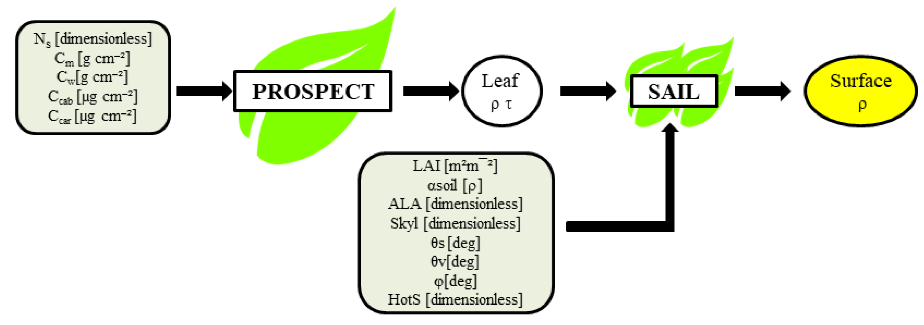
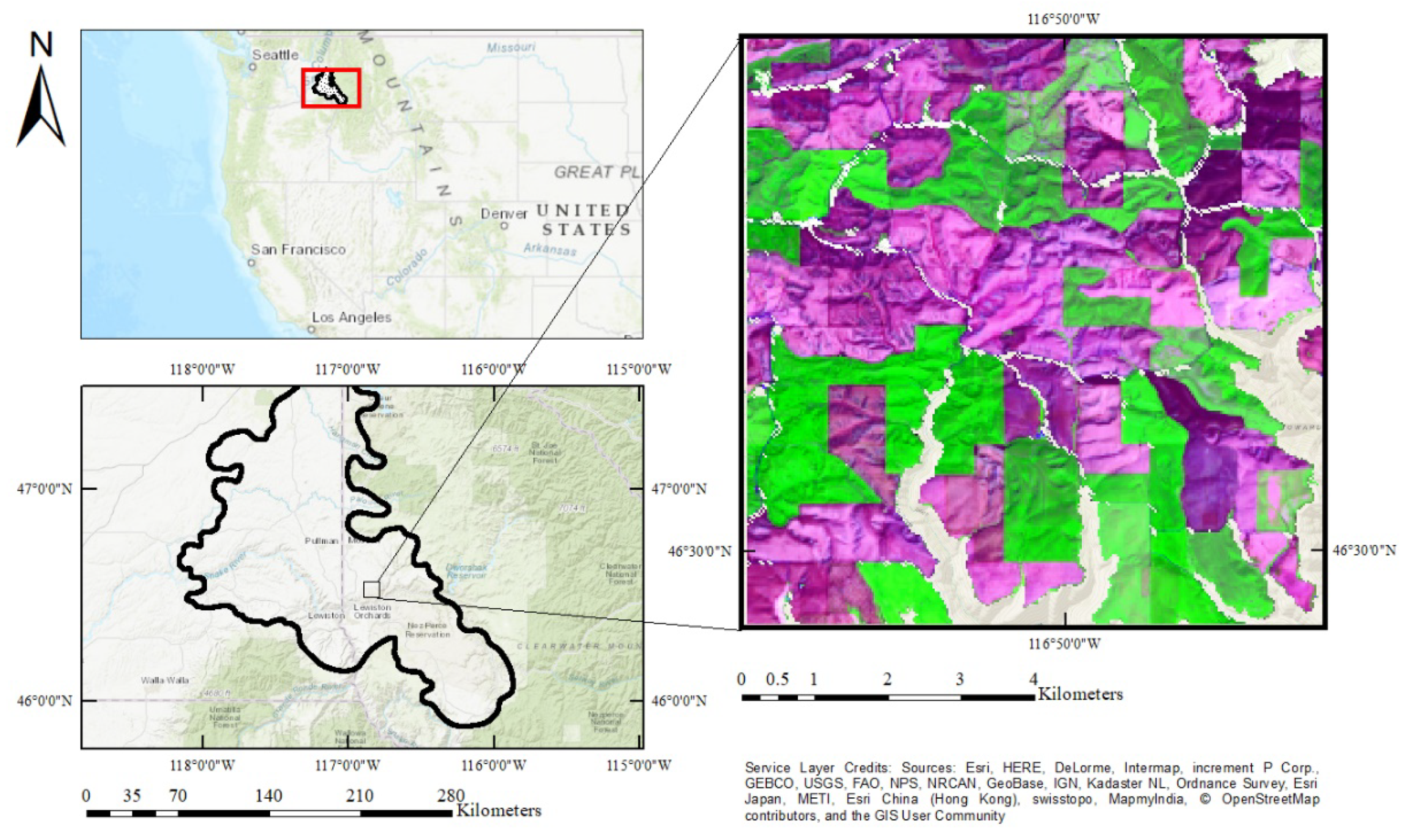
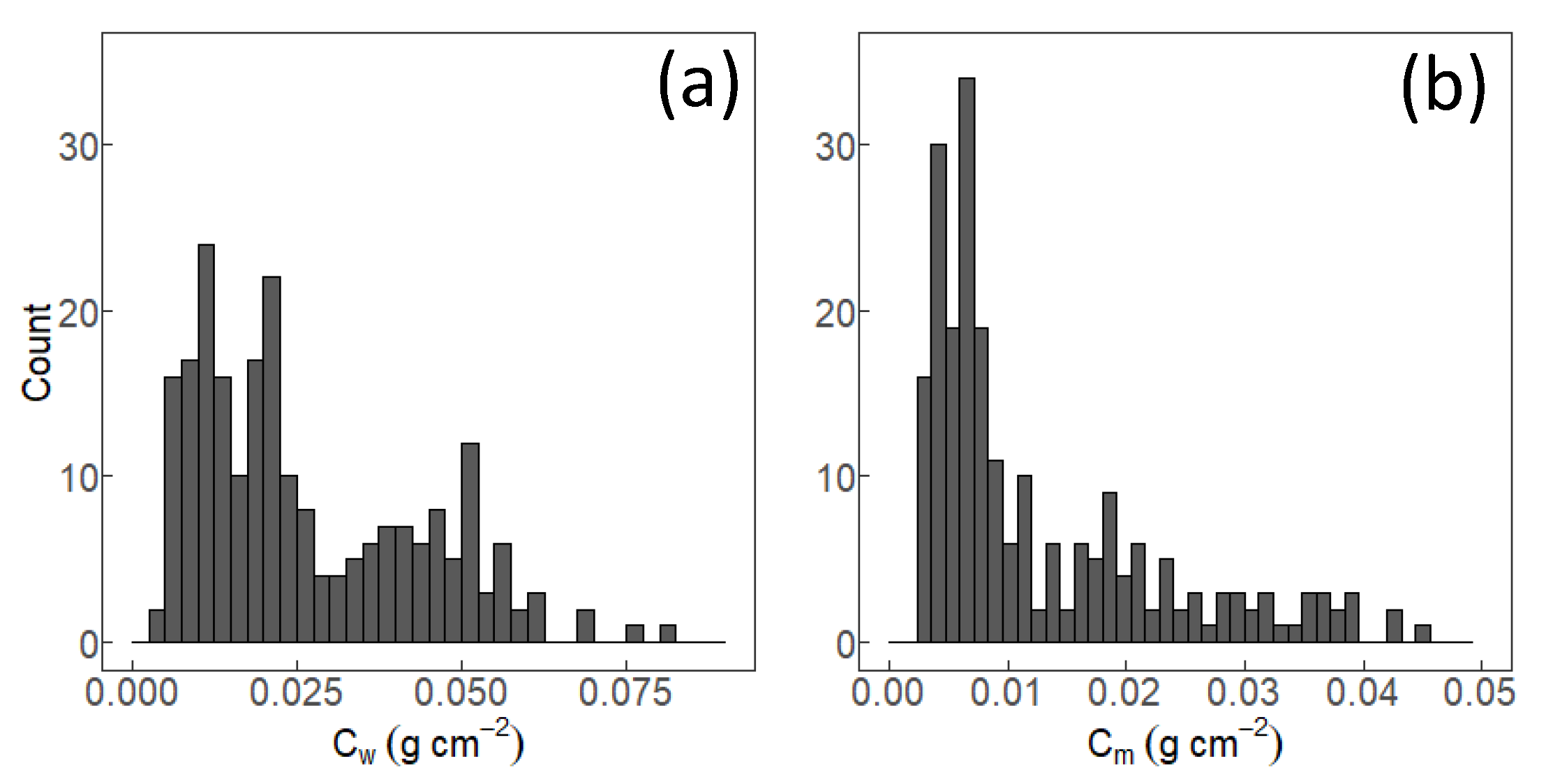
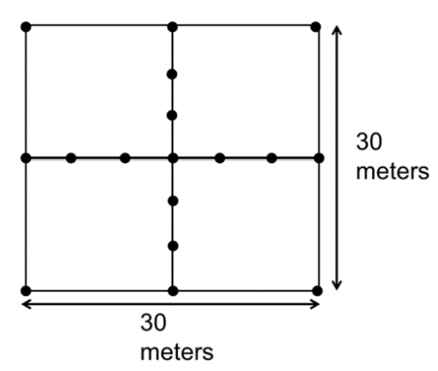
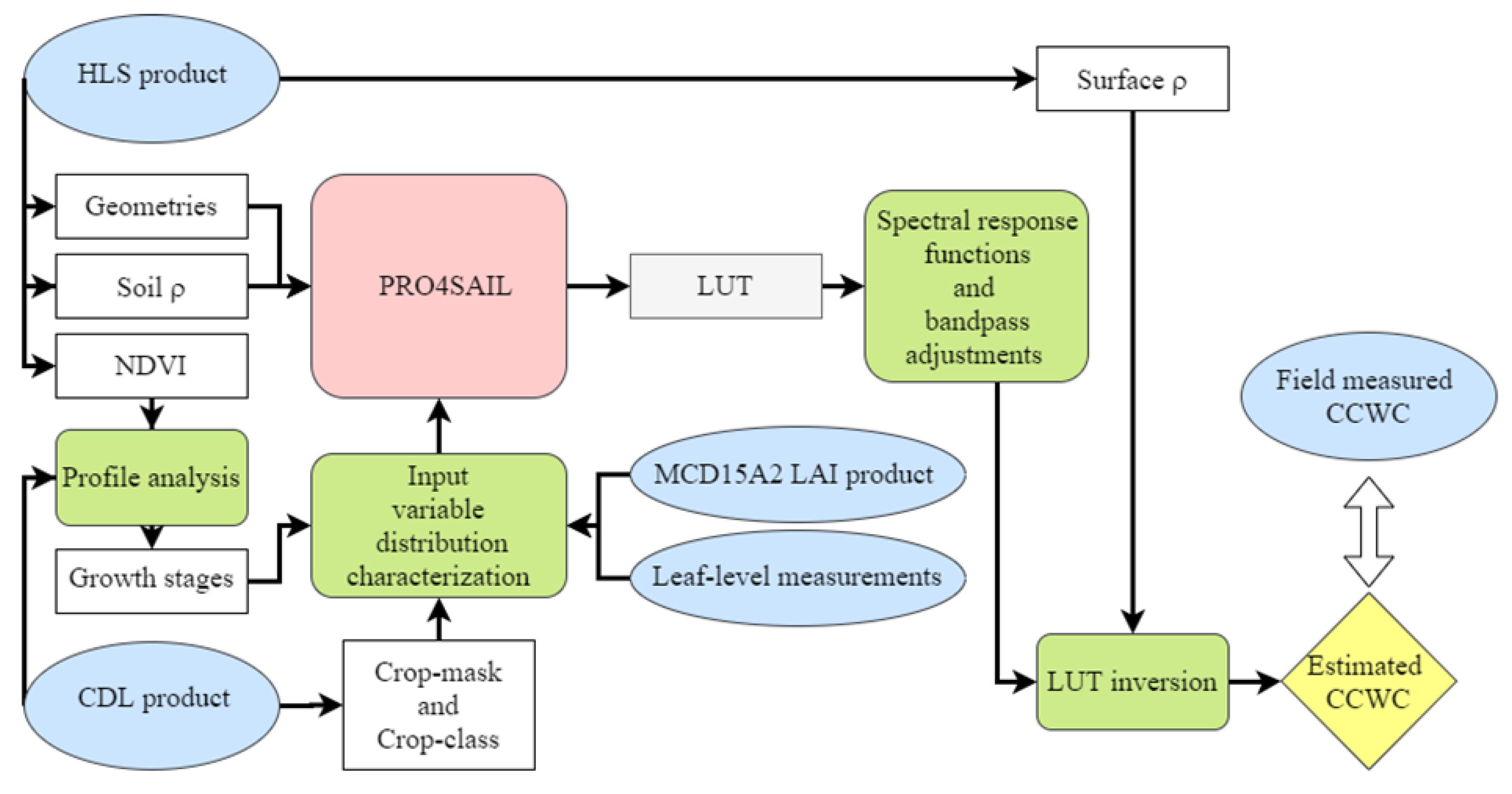
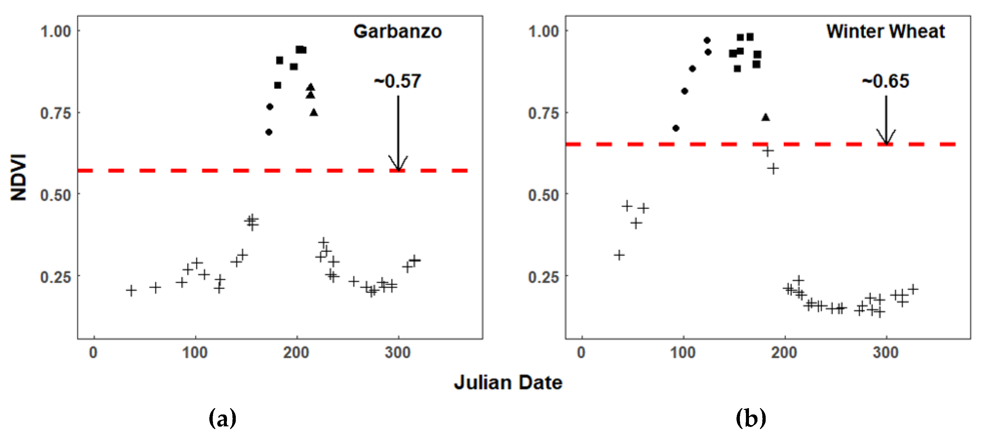
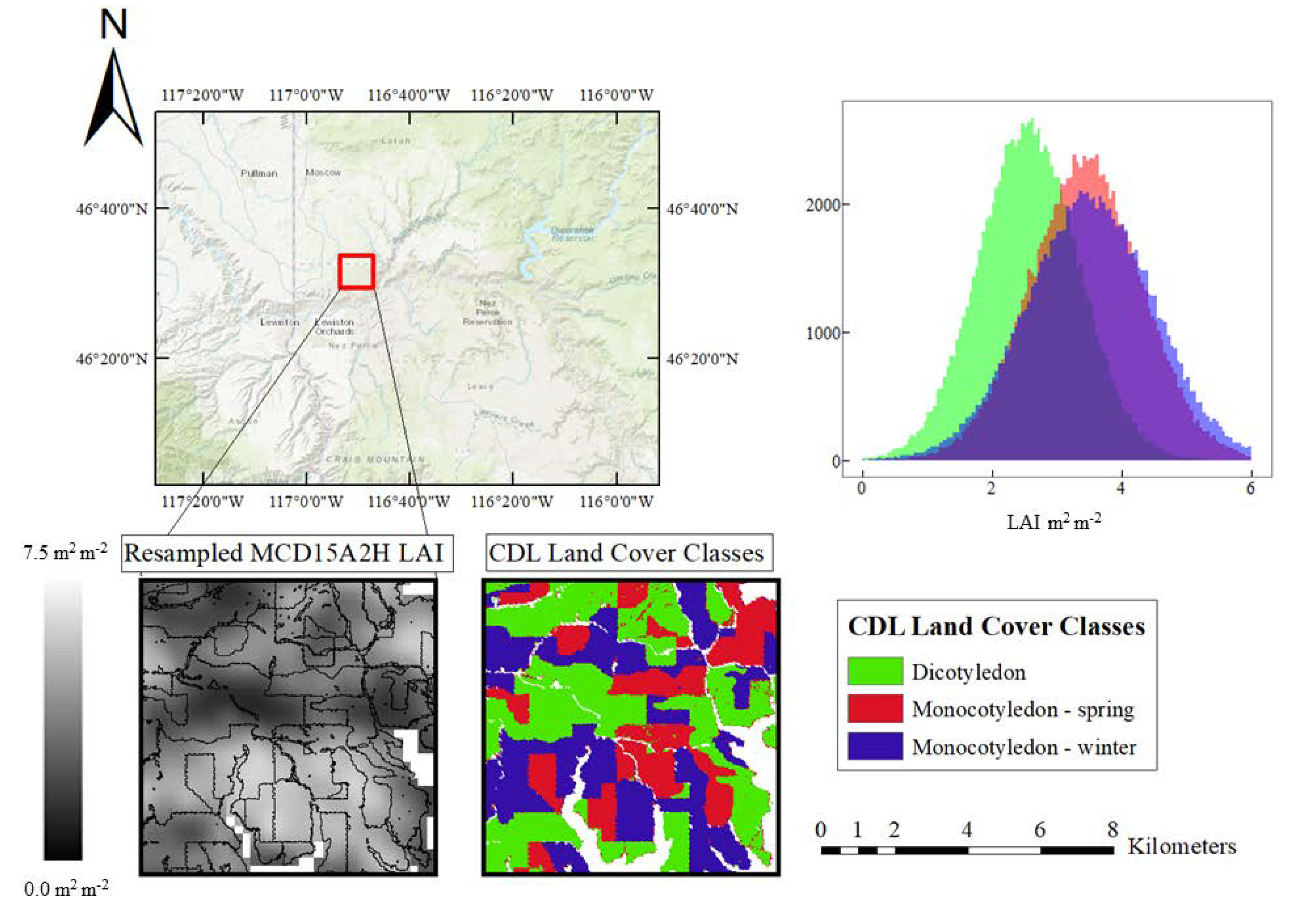
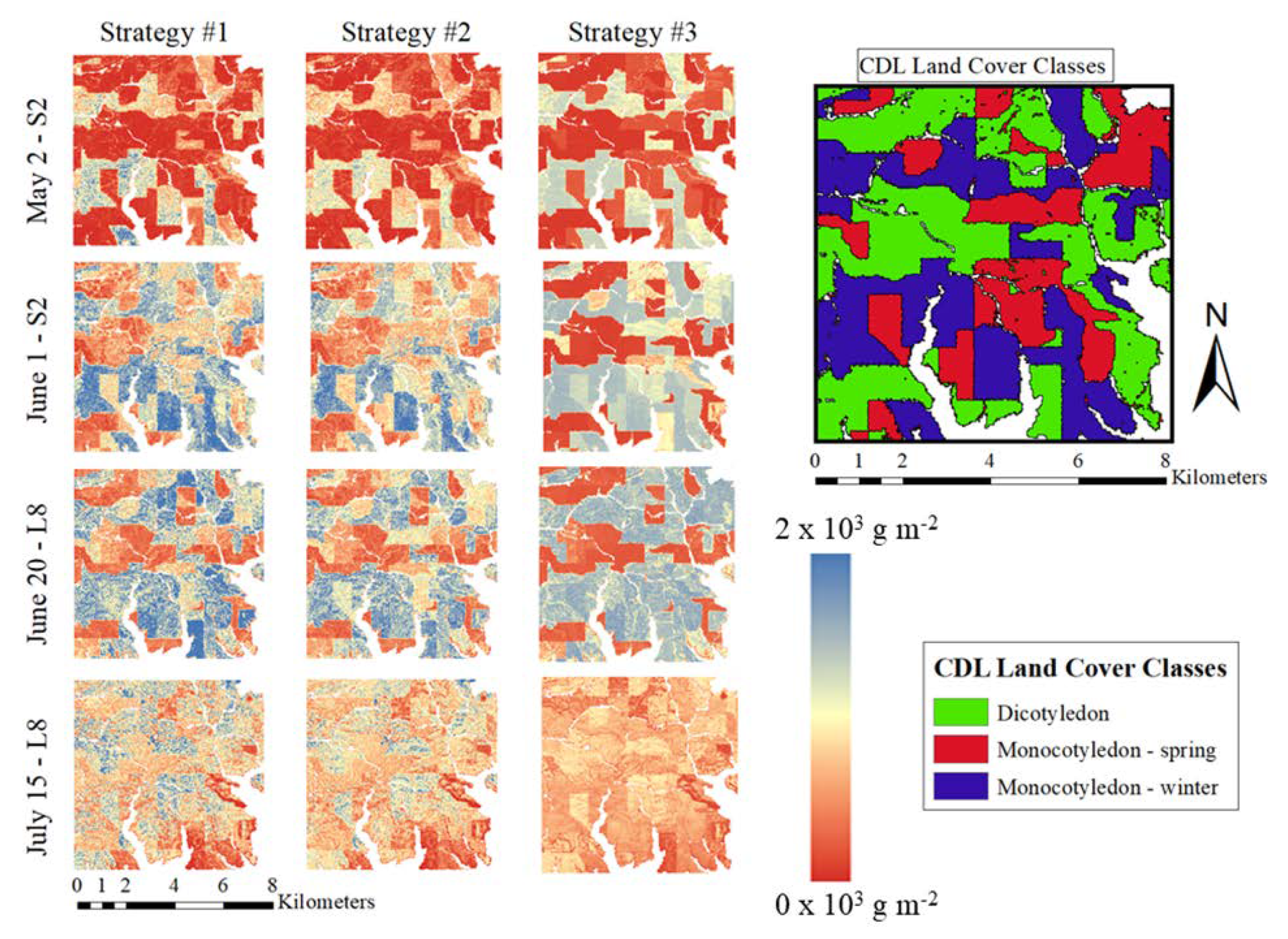
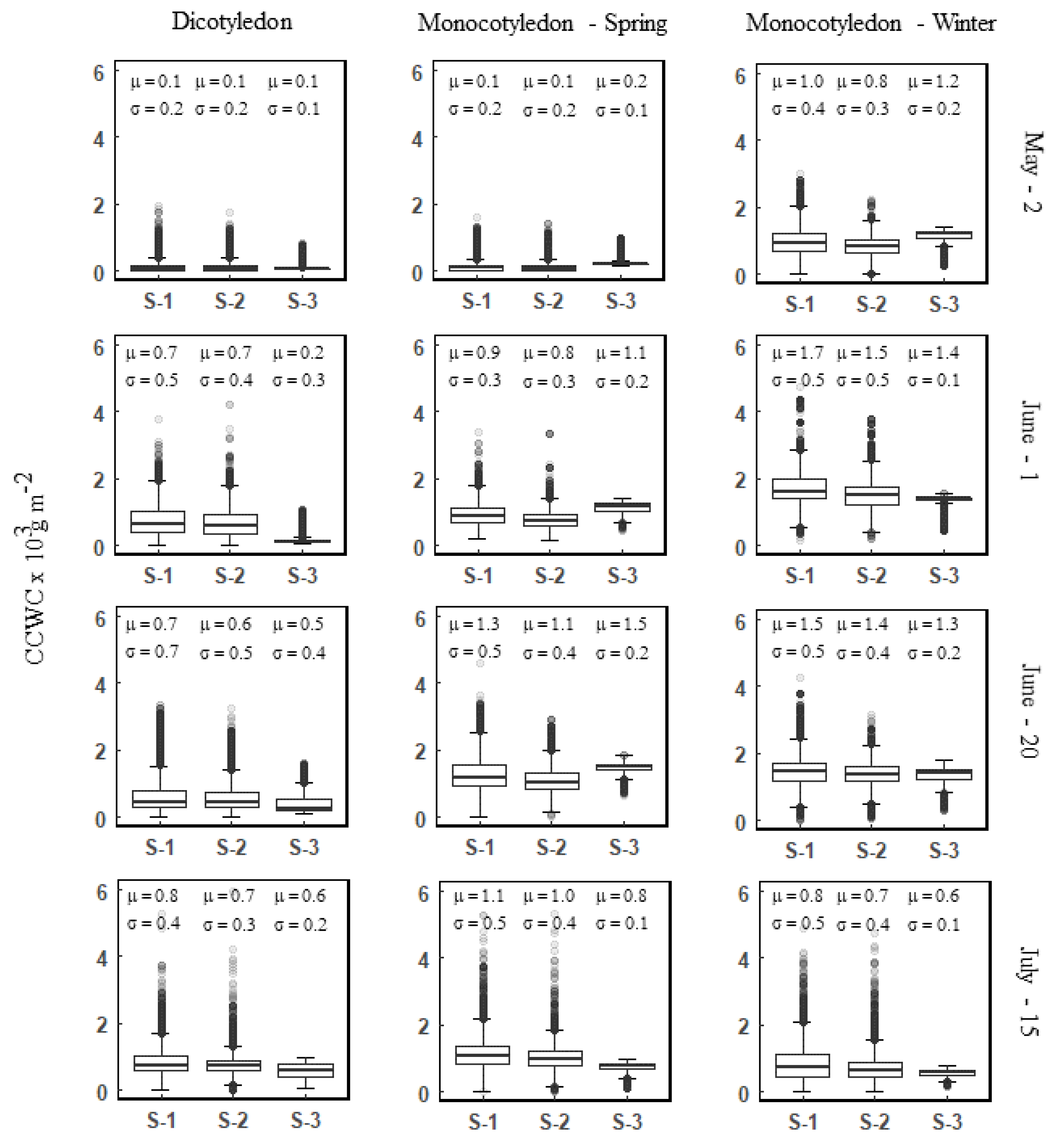
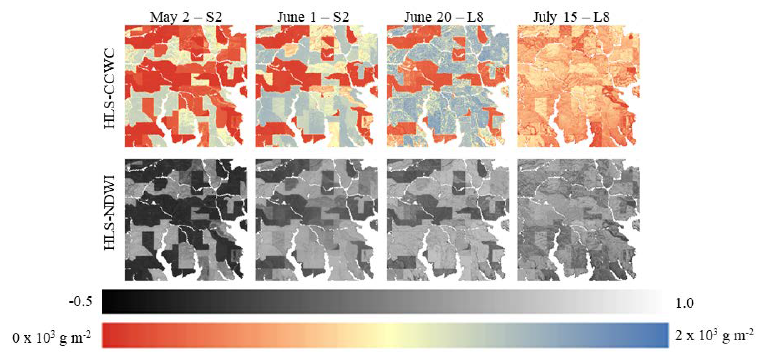
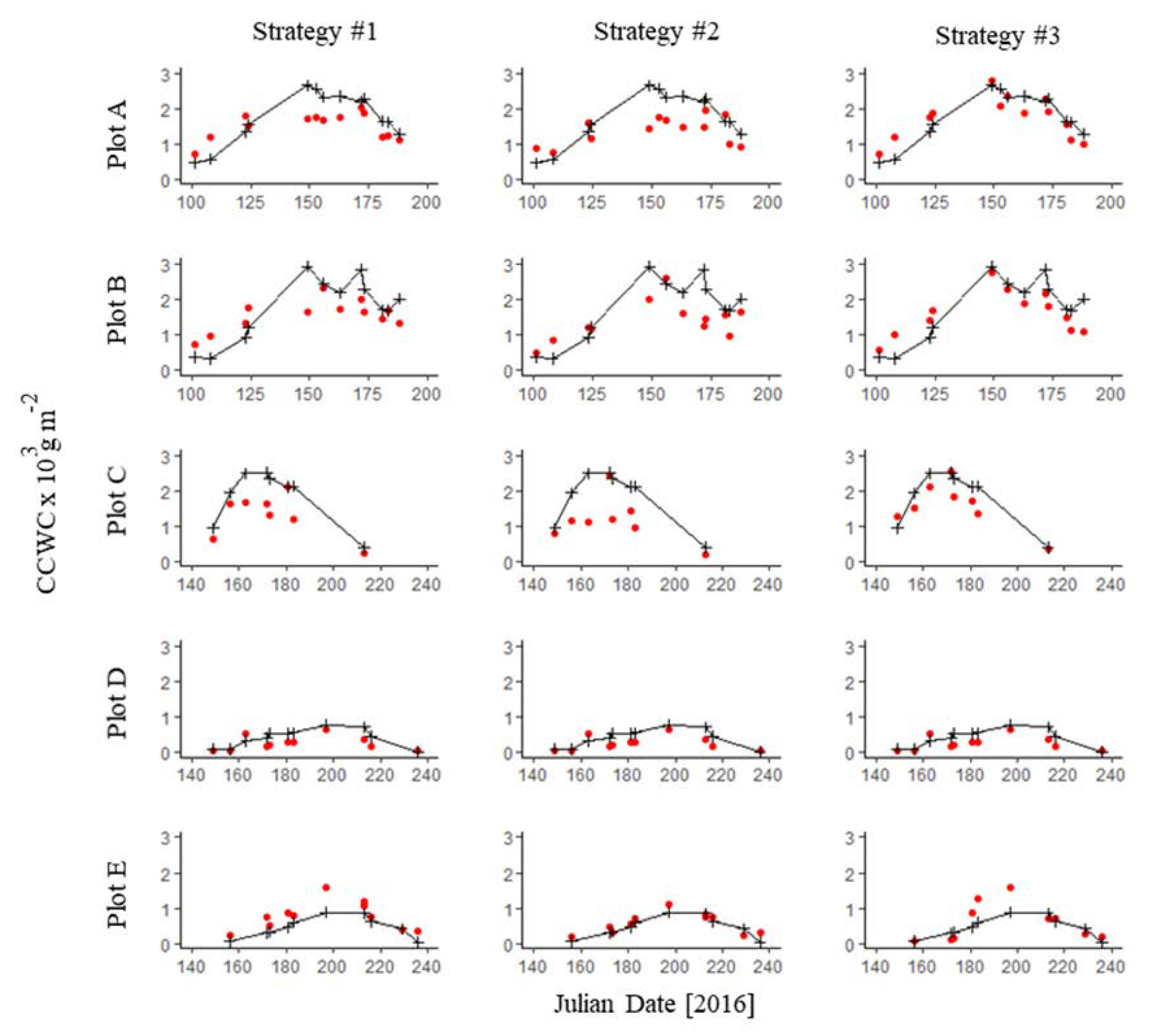
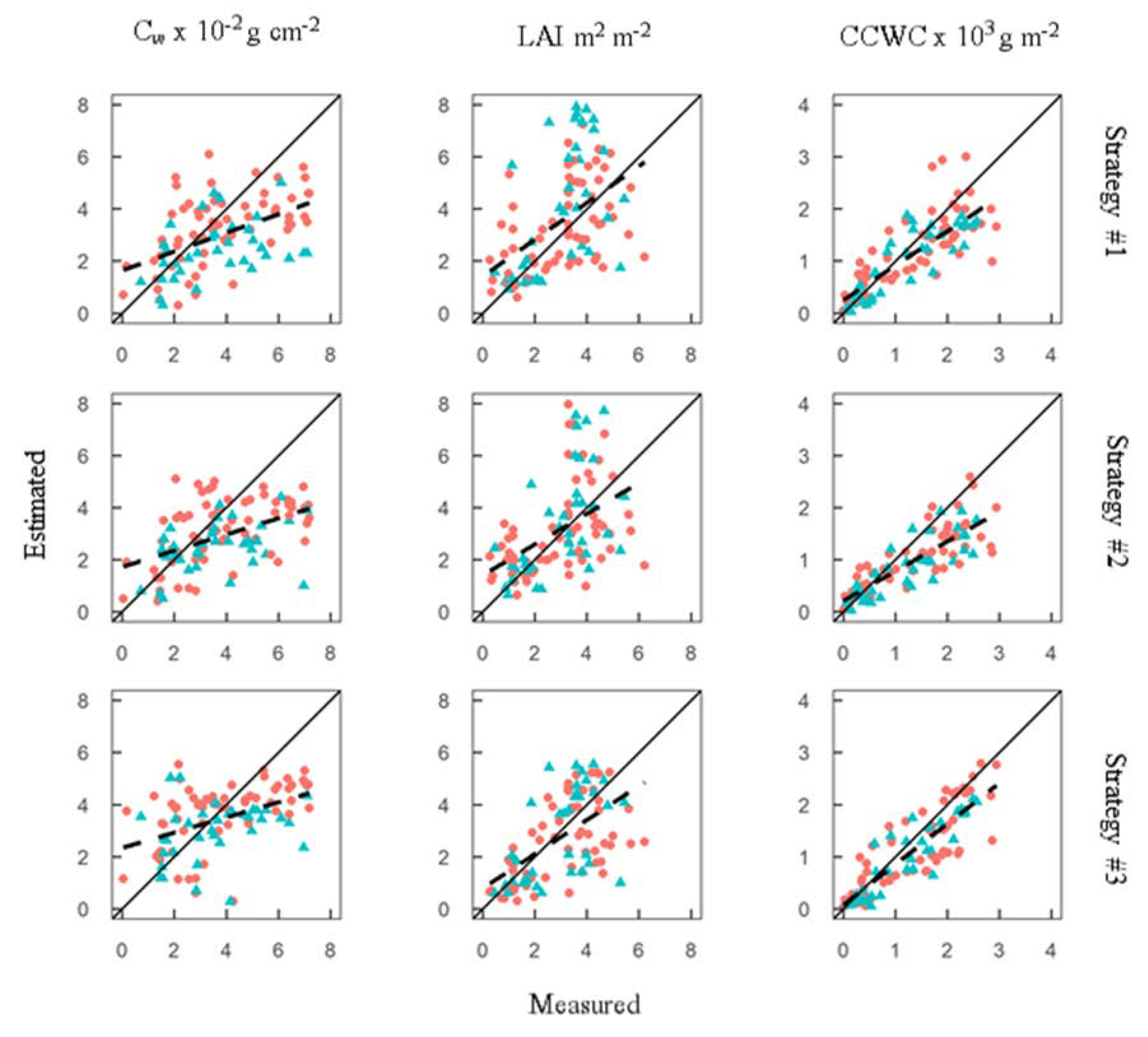
Table 1.
Harmonized Landsat Sentinel (HLS) product spectral bands. Table was adapted from [85].
Table 1.
Harmonized Landsat Sentinel (HLS) product spectral bands. Table was adapted from [85].
| Band name | OLI Band Number | MSI Band Number | Wavelength (µm) |
|---|---|---|---|
| Coastal Aerosol | 1 | 1 | 0.43–0.45 |
| Blue | 2 | 2 | 0.45–0.51 |
| Green | 3 | 3 | 0.53–0.59 |
| Red | 4 | 4 | 0.64–0.67 |
| Red-Edge1 | - | 5 | 0.69–0.71 |
| Red-Edge 2 | - | 6 | 0.73–0.75 |
| Red-Edge 3 | - | 7 | 0.77–0.79 |
| NIR Narrow | 5 | 8A | 0.85–0.88 |
| NIR Broad | - | 8 | 0.78–0.88 |
| SWIR 1 | 6 | 11 | 1.57–1.65 |
| SWIR 2 | 7 | 12 | 2.11–2.29 |
| Water vapor | - | 9 | 0.93–0.95 |
| Cirrus | 9 | 10 | 1.36–1.38 |
| Thermal Infrared 1 | 10 | - | 10.60–11.19 |
| QA |
Table 2.
Summary table of field sampling plots for each year.
| Year | Plot | Crop | Number of Field Measurements |
|---|---|---|---|
| 2015 | A | Barley | 4 |
| B | Barley | 3 | |
| C | Barley | 4 | |
| D | Barley | 4 | |
| E | Garbanzo | 3 | |
| 2016 | A | Winter Wheat | 13 |
| B | Winter Wheat | 12 | |
| C | Barley | 8 | |
| D | Garbanzo | 11 | |
| E | Garbanzo | 11 | |
| 2017 | A | Barley | 5 |
| B | Winter Wheat | 6 | |
| C | Winter Wheat | 6 | |
| D | Garbanzo | 6 | |
| E | Garbanzo | 6 |
Table 3.
Summary table of field sampling plots for each year, crop type, and sensor overpass.
| Total | Dicot | Mono. Winter | Mono. Spring | L8 Observations | S2 Observations | L8 | S2 | |
|---|---|---|---|---|---|---|---|---|
| 2015 | 18 | 3 | 0 | 15 | 18 | 0 | 5 | 0 |
| 2016 | 55 | 22 | 25 | 8 | 33 | 22 | 12 | 7 |
| 2017 | 29 | 12 | 12 | 5 | 15 | 14 | 3 | 4 |
| Total | 102 | 37 | 37 | 28 | 66 | 36 | 20 | 11 |
Table 4.
Parameterization of the PRO4SAIL radiative transfer model. The distributions used during LUT generation for each parameter are listed along with fixed values. The asterisk indicates that water thickness and dry matter content log-gaussian distributions in Strategy 3 were generated using a covariance matrix to simulate the correlation between water thickness and dry matter content. The covariances are presented in Table 5.
| Strategy 1 | Strategy 2 | Strategy 3 | |||
|---|---|---|---|---|---|
| Model Parameters | Symbol | Units | Parameter Values | ||
| Leaf Parameters PROSPECT-5 | |||||
| Leaf chlorophyll content | Ccab | µg cm−2 | Gaussian µ = 32.81, σ = 18.87 | Gaussian µ = 32.81, σ = 18.87 | Gaussian µ = 32.81, σ = 18.87 |
| Leaf carotenoid content | Ccar | µg cm−2 | Gaussian µ = 8.51, σ = 3.92 | Gaussian µ = 8.51, σ = 3.92 | Gaussian µ = 8.51, σ = 3.92 |
| Water thickness | Cw | g cm−2 | Gaussian µ = 0.027, σ = 0.018 | Gaussian µ = 0.027, σ = 0.018 | Log-Gaussian * µ = 0.027, σ = 0.018 |
| Dry matter content | Cm | g cm−2 | Gaussian µ = 0.013, σ = 0.01 | Gaussian µ = 0.013, σ = 0.01 | Log-Gaussian * µ = 0.013, σ = 0.01 |
| Leaf structure index | Ns | - | Uniform: 1.0–4.0 | Uniform: plant type and phenological stage dependent (Table 6) | Gaussian: plant type and phenological stage dependent (Table 6) |
| Canopy variables 4SAIL | |||||
| Leaf area index | LAI | m2 m−2 | Uniform: 0.0–8.0 | Uniform: 0.0–8.0 | Gaussian: plant type and date dependent |
| Average leaf angle | ALA | degree | Uniform: 30–70 | Uniform: 30–70 | Plant type dependent: Erectophile and Uniform |
| Soil coefficient | αsoil | unitless | Uniform: 0–1 | Uniform: 0–1 | Uniform: 0.3–0.7 |
Table 5.
Covariance matrix of Cw and Cm parameters used for LUT generation in strategy 3.
| Cw | Cm | |
| Cw | 3.2 × 10⁻⁴ | 1.5 × 10⁻⁴ |
| Cm | 1.5 × 10⁻⁴ | 1.0 × 10⁻⁴ |
Table 6.
Parameterization of the Ns parameter in PRO4SAIL. Values in the strategy 2 column were used as the minimum and maximum range bounds for generating uniform Ns values while the values in strategy 3 were used as the mean and standard deviation values for generating gaussian Ns values. Values based on Table 2 results in Boren et al. [88].
| Strategy 2 | Strategy 3 | |||
|---|---|---|---|---|
| Phenological Stage | Monocotyledon | Dicotyledon | Monocotyledon | Dicotyledon |
| Early | 1.0–1.5 | 2.0–2.5 | µ = 1.35, σ = 0.28 | µ = 2.15, σ = 0.27 |
| Mid | 1.5–2.0 | 2.0–2.5 | µ = 1.5, σ = 0.23 | µ = 1.96, σ = 0.25 |
| Late | 1.5–2.0 | 2.0–2.5 | µ = 1.66, σ = 0.25 | µ = 2.15, σ = 0.27 |
Table 7.
Phenological stages used for inversion strategies 2 and 3 for each crop type in Figure 8 images; early, mid, and late phenological stages correspond to emergence, establishment, and maturation.
Table 7.
Phenological stages used for inversion strategies 2 and 3 for each crop type in Figure 8 images; early, mid, and late phenological stages correspond to emergence, establishment, and maturation.
| Crop Type | 2-May | 1-June | 20-June | 15-July |
|---|---|---|---|---|
| Dicotyledon | Early | Early | Early | Late |
| Spring Monocotyledon | Early | Early | Mid | Late |
| Winter Monocotyledon | Early | Mid | Mid | Late |
Table 8.
Regression and validation metrics for LAI, Cw, and CCWC estimated through the three inversion strategies. The table presents the results obtained considering Landsat-8 (L8) data only, Sentinel-2A (S2) data only, and both sensors (L8/S2).
Table 8.
Regression and validation metrics for LAI, Cw, and CCWC estimated through the three inversion strategies. The table presents the results obtained considering Landsat-8 (L8) data only, Sentinel-2A (S2) data only, and both sensors (L8/S2).
| Cw (10−2g cm−2) | |||||||
| RMSE | MAE | NSE | Slope | Intercept | R2 | ||
| L8 | Strategy 1 | 1.90 | 1.50 | 0.19 | 0.35 | 1.89 | 0.30 |
| Strategy 2 | 2.01 | 1.56 | 0.07 | 0.29 | 1.97 | 0.24 | |
| Strategy 3 | 1.90 | 1.50 | 0.18 | 0.27 | 2.62 | 0.21 | |
| S2 | Strategy 1 | 2.30 | 1.70 | −0.39 | 0.17 | 1.80 | 0.10 |
| Strategy 2 | 2.20 | 1.57 | −0.26 | 0.19 | 1.77 | 0.16 | |
| Strategy 3 | 2.05 | 1.55 | −0.10 | 0.17 | 2.36 | 0.10 | |
| L8/S2 | Strategy 1 | 2.04 | 1.56 | 0.00 | 0.30 | 1.80 | 0.22 |
| Strategy 2 | 2.07 | 1.57 | −0.04 | 0.26 | 1.87 | 0.21 | |
| Strategy 3 | 1.95 | 1.53 | 0.09 | 0.24 | 2.49 | 0.17 | |
| LAI (m2 m−2) | |||||||
| RMSE | MAE | NSE | Slope | Intercept | R2 | ||
| L8 | Strategy 1 | 1.58 | 1.25 | −0.17 | 0.57 | 1.51 | 0.26 |
| Strategy 2 | 1.67 | 1.31 | −0.30 | 0.47 | 1.65 | 0.18 | |
| Strategy 3 | 1.42 | 1.14 | 0.06 | 0.61 | 0.86 | 0.33 | |
| S2 | Strategy 1 | 2.30 | 1.79 | −2.07 | 1.01 | 1.04 | 0.30 |
| Strategy 2 | 1.73 | 1.32 | −0.73 | 0.86 | 0.80 | 0.31 | |
| Strategy 3 | 1.44 | 1.12 | −0.19 | 0.76 | 0.61 | 0.34 | |
| L8/S2 | Strategy 1 | 1.87 | 1.44 | −0.75 | 0.71 | 1.41 | 0.25 |
| Strategy 2 | 1.69 | 1.31 | −0.43 | 0.59 | 1.41 | 0.22 | |
| Strategy 3 | 1.43 | 1.14 | −0.02 | 0.66 | 0.79 | 0.33 | |
| CCWC (103g m−2) | |||||||
| RMSE | MAE | NSE | Slope | Intercept | R2 | ||
| L8 | Strategy 1 | 0.56 | 0.43 | 0.59 | 0.66 | 0.28 | 0.63 |
| Strategy 2 | 0.59 | 0.44 | 0.56 | 0.57 | 0.24 | 0.71 | |
| Strategy 3 | 0.49 | 0.35 | 0.69 | 0.78 | 0.09 | 0.74 | |
| S2 | Strategy 1 | 0.46 | 0.37 | 0.66 | 0.66 | 0.21 | 0.73 |
| Strategy 2 | 0.57 | 0.43 | 0.48 | 0.57 | 0.16 | 0.69 | |
| Strategy 3 | 0.41 | 0.33 | 0.73 | 0.78 | 0.03 | 0.82 | |
| L8/S2 | Strategy 1 | 0.53 | 0.40 | 0.62 | 0.66 | 0.25 | 0.66 |
| Strategy 2 | 0.58 | 0.44 | 0.53 | 0.57 | 0.21 | 0.70 | |
| Strategy 3 | 0.46 | 0.34 | 0.71 | 0.78 | 0.07 | 0.76 | |
© 2020 by the authors. Licensee MDPI, Basel, Switzerland. This article is an open access article distributed under the terms and conditions of the Creative Commons Attribution (CC BY) license (http://creativecommons.org/licenses/by/4.0/).
Share and Cite
MDPI and ACS Style
Boren, E.J.; Boschetti, L. Landsat-8 and Sentinel-2 Canopy Water Content Estimation in Croplands through Radiative Transfer Model Inversion. Remote Sens. 2020, 12, 2803. https://0-doi-org.brum.beds.ac.uk/10.3390/rs12172803
AMA Style
Boren EJ, Boschetti L. Landsat-8 and Sentinel-2 Canopy Water Content Estimation in Croplands through Radiative Transfer Model Inversion. Remote Sensing. 2020; 12(17):2803. https://0-doi-org.brum.beds.ac.uk/10.3390/rs12172803
Chicago/Turabian StyleBoren, Erik J., and Luigi Boschetti. 2020. "Landsat-8 and Sentinel-2 Canopy Water Content Estimation in Croplands through Radiative Transfer Model Inversion" Remote Sensing 12, no. 17: 2803. https://0-doi-org.brum.beds.ac.uk/10.3390/rs12172803
Note that from the first issue of 2016, this journal uses article numbers instead of page numbers. See further details here.