A Comparison of Three Temporal Smoothing Algorithms to Improve Land Cover Classification: A Case Study from NEPAL

 , ,
, ,  , , and
Abstract
:
1. Introduction
2. Materials and Methods
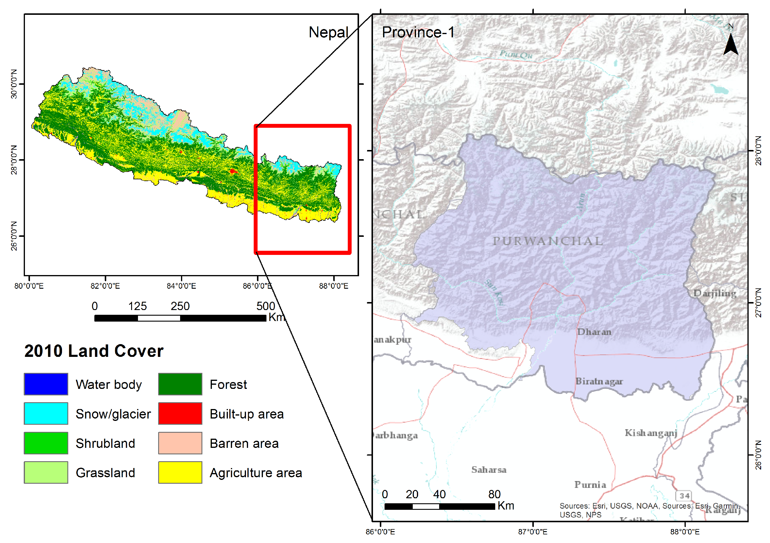
2.1. Study Area
2.2. Land Cover Typology
2.3. Reference Data Collection
2.4. Land Cover Classification
2.4.1. Optical Image Processing
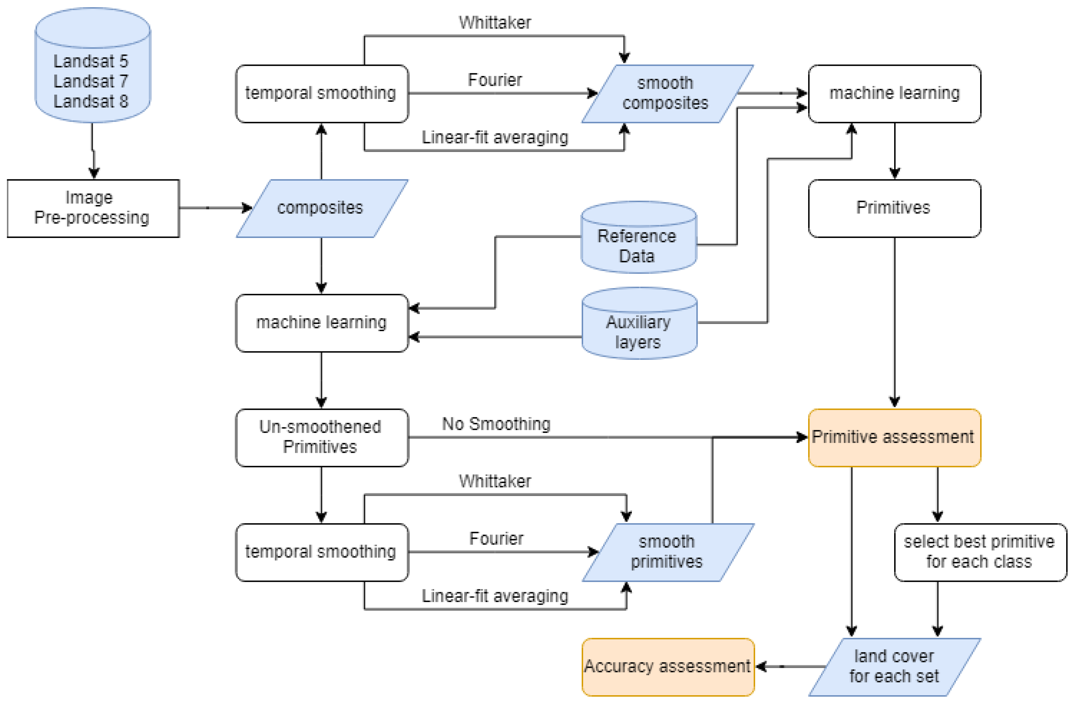
2.4.2. Application of Smoothing
2.4.3. Final Land Cover Map Generation and Accuracy Assessment
3. Results
4. Discussion
5. Conclusions
Author Contributions
Funding
Acknowledgments
Conflicts of Interest
Appendix A. Reference Data

| Land Class | Training Points | Validation Points |
|---|---|---|
| bare | 1272 | 545 |
| cropland | 29,537 | 600 |
| forest | 45,806 | 600 |
| grassland | 378 | 162 |
| riverBed | 1615 | 600 |
| settlement | 1501 | 600 |
| snow | 3565 | 600 |
| wetland | 2419 | 600 |
Appendix B. Smoothing Codes
Appendix B.1. Smoothing Composites
- 1
- DESCRIPTION
- 2
- 3
- In order to test the impact of smoothing in landcover classification, we need to
- 4
- first
- 5
- check with smoothing the surface reflectance itself as well as smoothing the
- 6
- intermediate smoothing results. In this step we will be smoothing composites
- 7
- themself
- 8
- using different algorithms namely whittaker, fourier and linear fit.
- 9
- 10
- SCRIPT INFO
- 11
- 12
- The users can/should change the following
- 13
- 1. imageCollection - source image collection that needs to be smoothened
- 14
- 2. boundary - the study region
- 15
- 3. smoothingAlgorithm - the algorithm to perform smoothing. can be ’whittaker’,
- 16
- ’fourier’
- 17
- or ’linearFit’
- 18
- 3. startYear - the start year from when to perform temporal smoothing
- 19
- 4. endYear - the end year to which to perform temporal smoothing
- 20
- 5. exportPath - the collection in which smoothened images are exported
- 21
- 22
- DEVELOPER NOTES
- 23
- 1. Make sure the masks in each region is common to avoid errors
- 24
- 25
- 26
- AUTHOR
- 27
- Nishanta Khanal
- 28
- ICIMOD, 2019
- 29
- */
- 30
- 31
- var imageCollection =
- 32
- ee.ImageCollection(’projects/servir-hkh/ncomp_yearly_30/compositesV2’);
- 33
- var boundary = ee.FeatureCollection(’users/nkhanal/boundaries/p1_buffer_2000’);
- 34
- var smoothingAlgorithm = "fourier";
- 35
- var startYear = 2000;
- 36
- var endYear = 2018;
- 37
- var exportPath = ’users/nkhanal/sm/four/comp’;
- 38
- 39
- 40
- var addCovariates =
- 41
- require("users/khanalnishant/ICIMOD:RLCMS/V2/Training/1_addCovariates_yearly")
- 42
- 43
- var smoothing = require("users/khanalnishant/EETest:Algo/WhittakerSmoothing")
- 44
- var param = 10;
- 45
- if(smoothingAlgorithm == ’fourier’){
- 46
- smoothing = require("users/khanalnishant/EETest:Algo/FourierSmoothing");
- 47
- param = false;
- 48
- }else if (smoothingAlgorithm == ’linearFit’){
- 49
- smoothing = require("users/khanalnishant/Algorithms:LinearFitSmoothing");
- 50
- param = 420;
- 51
- }
- 52
- 53
- 54
- 55
- // #####################################3
- 56
- // # perform smoothing
- 57
- // #####################################3
- 58
- // #add image attribures for smoothing
- 59
- function prepareImage(image){
- 60
- var imgYear = ee.Number.parse(image.id())
- 61
- image = image.unmask(0).clip(boundary).toShort()
- 62
- return image.set(’year’, imgYear,
- 63
- ’system:time_start’, ee.Date.fromYMD(imgYear, 1, 1).millis());
- 64
- }
- 65
- var imageCollection = imageCollection.map(prepareImage)
- 66
- print(imageCollection.first())
- 67
- 68
- // # get original band names and add fitted at end to select fitted bands
- 69
- var bandNames = ee.Image(imageCollection.first()).bandNames()
- 70
- function fittedName(band){
- 71
- return ee.String(band).cat(’_fitted’)
- 72
- }
- 73
- var fittedNames = bandNames.map(fittedName)
- 74
- 75
- var smoothingResults = smoothing.runModel(imageCollection, param)
- 76
- var imageCollection = smoothingResults[0].select(fittedNames, bandNames)
- 77
- var rmse = smoothingResults[1]
- 78
- 79
- function exportHelper(image, assetID, imageCollectionID){
- 80
- image = image.int16()
- 81
- // # image = setExportProperties(image, args)
- 82
- 83
- Export.image.toAsset({
- 84
- image:ee.Image(image),
- 85
- description:smoothingAlgorithm+"-"+assetID +"-from-js",
- 86
- assetId:imageCollectionID+’/’+assetID,
- 87
- region:boundary,
- 88
- maxPixels:1e13,
- 89
- scale: 30
- 90
- });
- 91
- }
- 92
- 93
- for (var year=startYear;year<=endYear;year++){
- 94
- var image = ee.Image(imageCollection.filter(ee.Filter.eq(’year’,year)).first())
- 95
- .clip(boundary)
- 96
- exportHelper(image, year, exportPath)
- 97
- }
- 98
- 99
- Export.image.toAsset({
- 100
- image:ee.Image(rmse),
- 101
- description:smoothingAlgorithm+"-rmse-from-js",
- 102
- assetId:exportPath+’/rmse’,
- 103
- region:boundary,
- 104
- maxPixels:1e13,
- 105
- scale: 30
- 106
- });
Appendix B.2. Smoothing Primitives
- 1
- /*
- 2
- DESCRIPTION
- 3
- 4
- In order to test the impact of smoothing landcover classification, we need to
- 5
- first check with smoothing the surface reflectance itself as well as smoothing the
- 6
- intermediate smoothing results. In this step we will be smoothing primitives using
- 7
- different algorithms namely whittaker, fourier and linear fit. The export will
- 8
- generate an image with timeseries data and rmse on different bands. Different
- 9
- script is later required to split them into images.
- 10
- 11
- SCRIPT INFO
- 12
- 13
- The users can/should change the following
- 14
- 1. imageCollection - source image collection that contains the unsmoothened
- 15
- primitives
- 16
- 2. primitive - the primitive to be smoothened
- 17
- 3. boundary - the study region
- 18
- 4. smoothingAlgorithm - the algorithm to perform smoothing. can be ’whittaker’,
- 19
- ’fourier’ or ’linearFit’
- 20
- 5. startYear - the start year from when to perform temporal smoothing
- 21
- 6. endYear - the end year to which to perform temporal smoothing
- 22
- 7. exportPath - the collection in which smoothened images are exported
- 23
- 24
- DEVELOPER NOTES
- 25
- 1. Make sure the masks in each region is common to avoid errors
- 26
- 27
- AUTHOR
- 28
- Nishanta Khanal
- 29
- ICIMOD, 2019
- 30
- */
- 31
- 32
- var imageCollectionId = ’users/nkhanal/sm/nosm/prims’;
- 33
- var primitive = ’wetland’
- 34
- var boundary = ee.FeatureCollection(’users/nkhanal/boundaries/p1_buffer_2000’);
- 35
- var smoothingAlgorithm = "linearFit";
- 36
- var startYear = 2000;
- 37
- var endYear = 2018;
- 38
- var exportPath = ’users/nkhanal/sm/line/primtemp’;
- 39
- 40
- var addCovariates =
- 41
- require("users/khanalnishant/ICIMOD:RLCMS/V2/Training/1_addCovariates_yearly")
- 42
- 43
- var smoothing = require("users/khanalnishant/EETest:Algo/WhittakerSmoothing")
- 44
- var param = 10;
- 45
- if(smoothingAlgorithm == ’fourier’){
- 46
- smoothing = require("users/khanalnishant/EETest:Algo/FourierSmoothing");
- 47
- param = false;
- 48
- }else if (smoothingAlgorithm == ’linearFit’){
- 49
- smoothing = require("users/khanalnishant/Algorithms:LinearFitSmoothing");
- 50
- param = 420;
- 51
- }
- 52
- 53
- 54
- // #####################################3
- 55
- // # perform smoothing
- 56
- // #####################################3
- 57
- // #add image attribures for smoothing
- 58
- var yearlyPrims = [];
- 59
- for (var year = startYear; year<=endYear; year++){
- 60
- var image = ee.Image(imageCollectionId+’/’+primitive+’-’+year).unmask(0)
- 61
- .clip(boundary);
- 62
- image = image.set(’year’, year,
- 63
- ’system:time_start’, ee.Date.fromYMD(year, 1, 1).millis())
- 64
- yearlyPrims.push(image);
- 65
- }
- 66
- imageCollection = ee.ImageCollection(yearlyPrims);
- 67
- print(imageCollection.first())
- 68
- 69
- // # get original band names and add fitted at end to select fitted bands
- 70
- var bandNames = ee.Image(imageCollection.first()).bandNames()
- 71
- function fittedName(band){
- 72
- return ee.String(band).cat(’_fitted’)
- 73
- }
- 74
- var fittedNames = bandNames.map(fittedName)
- 75
- 76
- var smoothingResults = smoothing.runModel(imageCollection, param)
- 77
- var imageCollection = smoothingResults[0].select(fittedNames, bandNames)
- 78
- var rmse = smoothingResults[1]
- 79
- 80
- function exportHelper(image, assetID, exportPath){
- 81
- image = image.int16()
- 82
- Export.image.toAsset({
- 83
- image:ee.Image(image),
- 84
- description:smoothingAlgorithm+"-"+assetID +"-from-js",
- 85
- assetId:exportPath+’/’+primitive+’-’+assetID,
- 86
- region:boundary,
- 87
- maxPixels:1e13,
- 88
- scale: 30
- 89
- });
- 90
- }
- 91
- 92
- var img = ee.Image([])
- 93
- for (var year=startYear;year<=endYear;year++){
- 94
- var image = ee.Image(imageCollection.filter(ee.Filter.eq(’year’,year)).first())
- 95
- .clip(boundary)
- 96
- img = img.addBands(image.rename(’b’+year));
- 97
- }
- 98
- var img = img.addBands(rmse.rename(’rmse’)).toInt16();
- 99
- 100
- Export.image.toAsset({
- 101
- image:img,
- 102
- description:smoothingAlgorithm+"-"+primitive+"-from-js",
- 103
- assetId:exportPath+’/’+primitive+’Results’,
- 104
- region:boundary,
- 105
- maxPixels:1e13,
- 106
- scale: 30
- 107
- });
Appendix B.3. Assemblage
- 1
- /*
- 2
- DESCRIPTION
- 3
- 4
- Now that we have satisfactory primitives we will run them through assembler
- 5
- to obtain a land cover map. The assembler prepares a decision tree based on
- 6
- user specified thresholds which can be tuned based on visual assessment as
- 7
- well as primitive assessment plots. The order of primitives in the list denotes
- 8
- the order in which primitives are placed in the decision tree with the first
- 9
- primitive placed on the top and so forth. This basically means that if a pixel
- 10
- has high probability on two primitives (according to the specified threshold)
- 11
- the final class will be based on the primitive that is higher up on the decision
- 12
- tree.
- 13
- 14
- SCRIPT INFOS
- 15
- 16
- The users can/should change the following parameters.
- 17
- 1. boundary - this should contain the boundary of region of interest
- 18
- 2. repository - the repository that contains the stack of primitives required
- 19
- 3. scale - the spatial resolution of the resulting landCover
- 20
- 4. exportPath - the path to which to export the resulting landcover
- 21
- 5. primitives - the list of primitives to include in the assembler
- 22
- 6. defaultThresholds - (optional) the default thresholds that the interface
- 23
- initiates with.It can be changed in the UI later. This should be in line
- 24
- with the list of primitives.
- 25
- 7. year - (optional) the default year to load into the interface
- 26
- 27
- The users need to do the following
- 28
- 1. After the script is run, initiate the export task by going to the "Tasks" tab
- 29
- ------->>>>>>>
- 30
- 31
- */
- 32
- 33
- /*
- 34
- Variables - refer above notes section for description on these
- 35
- */
- 36
- var boundary = ee.FeatureCollection("users/nkhanal/boundaries/p1_buffer_2000")
- 37
- .geometry();
- 38
- var repository = ’users/nkhanal/sm/final/prims/’;
- 39
- var scale = 30;
- 40
- var exportPath = ’users/nkhanal/sm/final/lc’;
- 41
- var primitives = [’snow’,’forest’,’cropland’,’wetland’,’riverBed’,’settlement’,
- 42
- ’bare’];
- 43
- var defaultThresholds = [70, 60, 60, 65, 60, 60, 70];
- 44
- var year = 2017;
- 45
- 46
- /* -------------------------------------------------------------------------------
- 47
- WARNING!!!
- 48
- 49
- FUNCTIONS AND PROCEDURES BELOW HERE
- 50
- 51
- edit at your own risk
- 52
- */
- 53
- 54
- // container for the classified landclass image
- 55
- var landClass = ee.Image();
- 56
- 57
- // ************************************************
- 58
- // ui objects
- 59
- // containers for sliders
- 60
- var sliders = {};
- 61
- // containers for inspected values
- 62
- var valLabels = {};
- 63
- // list of all selectable years
- 64
- var availableYears = [’2000’,’2001’,’2002’,’2003’,’2004’,’2005’,
- 65
- ’2006’,’2007’,’2008’,’2009’,’2010’,’2011’,
- 66
- ’2012’,’2013’,’2014’,’2015’,’2016’,’2017’,’2018’];
- 67
- // dropdown to select years
- 68
- var yearList = ui.Select(availableYears, ’year’, ’’+year);
- 69
- // checkbox to visualize primitives using thresholds
- 70
- var primThresholds = ui.Checkbox({
- 71
- label:’Visualize primitive by thresholds’,
- 72
- style:{’height’:’18px’,’fontSize’:’11px’, ’padding’:’4px’, ’margin’:’0px’}
- 73
- });
- 74
- // button to refresh display according to parameters
- 75
- var refreshDisplay = ui.Button({
- 76
- label:’Refresh Display’,
- 77
- onClick: refresh,
- 78
- style: {’fontSize’:’11px’, ’padding’:’4px’, ’margin’:’0px’}
- 79
- });
- 80
- // button to export the current LandCover
- 81
- var exportLC = ui.Button({
- 82
- label:’Export current landCover’,
- 83
- onClick: exportHelper,
- 84
- style: {’fontSize’:’11px’, ’padding’:’4px’, ’margin’:’0px’}
- 85
- });
- 86
- // button to export the current LandCover
- 87
- var exportAllLC = ui.Button({
- 88
- label:’Export landcover stack’,
- 89
- onClick: exportAllHelper,
- 90
- style: {’fontSize’:’11px’, ’padding’:’4px’, ’margin’:’0px’}
- 91
- });
- 92
- // button to export problem regions
- 93
- var exportPA = ui.Button({
- 94
- label:’Export Problem Regions’,
- 95
- onClick: exportAreas,
- 96
- style: {’fontSize’:’11px’, ’padding’:’4px’, ’margin’:’0px’}
- 97
- });
- 98
- 99
- // ************************************************
- 100
- // functions
- 101
- 102
- // function to reclassify stack image using decision tree
- 103
- function reclassify(stackImage, decisionTree){
- 104
- var classifier = ee.Classifier.decisionTree(decisionTree);
- 105
- var landClass = stackImage.classify(classifier);
- 106
- return landClass;
- 107
- }
- 108
- 109
- // client side list map function to change list of primitives
- 110
- // to a list of images corresponding to the primitives
- 111
- // also adds the primitives to the map
- 112
- function getPrimitiveImages(primitive){
- 113
- var image = ee.Image(repository+primitive).select(’b’+year)
- 114
- ;.multiply(0.01)
- 115
- .rename(primitive);
- 116
- var primLayer = ui.Map.Layer(image, {max:100}, primitive, false, 1);
- 117
- if (primThresholds.getValue()){
- 118
- primLayer = ui.Map.Layer(image.gte(sliders[primitive].getValue()),
- 119
- {},
- 120
- primitive,
- 121
- false,
- 122
- 1);
- 123
- }
- 124
- Map.layers().set(primitives.indexOf(primitive), primLayer);
- 125
- return image;
- 126
- }
- 127
- 128
- // function to build decision tree from interface
- 129
- function buildDecisionTree(){
- 130
- var values = {
- 131
- forest:sliders[’forest’].getValue(),
- 132
- wetland:sliders[’wetland’].getValue(),
- 133
- settlement:sliders[’settlement’].getValue(),
- 134
- cropland:sliders[’cropland’].getValue(),
- 135
- snow:sliders[’snow’].getValue(),
- 136
- riverBed:sliders[’riverBed’].getValue(),
- 137
- bare:sliders[’bare’].getValue()
- 138
- }
- 139
- 140
- var DT = [’1) root 9999 9999 9999’]
- 141
- var base = 1;
- 142
- for (var i = 0; i < primitives.length; i++){
- 143
- var a = base * 2
- 144
- var b = base * 2 + 1
- 145
- DT.push(’’+a+’) ’+
- 146
- primitives[i]+’>=’+values[primitives[i]]+
- 147
- ’ 9999 9999 ’+(i+1)+’ *’);
- 148
- if(i == primitives.length-1){
- 149
- DT.push(’’+b+’) ’+primitives[i]+’<’+values[primitives[i]]+’ 9999 9999 8 *’);
- 150
- }else DT.push(’’+b+’) ’+primitives[i]+’<’+values[primitives[i]]+’ 9999 9999 9999’);
- 151
- base = b
- 152
- }
- 153
- return DT.join(’\n’)
- 154
- }
- 155
- 156
- // function to start the process
- 157
- function process(year){
- 158
- var stackImage = ee.Image(primitives.map(getPrimitiveImages)).clip(boundary);
- 159
- landClass = reclassify(stackImage, buildDecisionTree());
- 160
- var lcLayer = ui.Map.Layer(landClass, imageVisParam, ’land cover’, true, 1);
- 161
- Map.layers().set(primitives.length, lcLayer);
- 162
- }
- 163
- 164
- // function to add legend to the map
- 165
- function addLegend(){
- 166
- var UTILS = require(’users/khanalnishant/Algorithms:Utilities’)
- 167
- var palette = imageVisParam.palette
- 168
- palette = palette
- 169
- var labels = primitives.concat(’grassland’)
- 170
- UTILS.addLegend(palette, labels,’Legend’,{
- 171
- ’position’:’bottom-right’,
- 172
- ’padding’:’8px 16px’,
- 173
- });
- 174
- }
- 175
- 176
- // function to add inspect panel to the map
- 177
- function addInspect(){
- 178
- var panel = ui.Panel([],
- 179
- ui.Panel.Layout.Flow(’vertical’),
- 180
- {maxHeight:’200px’,position:’bottom-center’});
- 181
- var inspectLabel = ui.Label(’Click to inspect primitive values’,
- 182
- {’height’:’18px’,
- 183
- ’fontSize’:’11px’,
- 184
- ’padding’:’0px’,
- 185
- ’margin’:’1px’});
- 186
- panel.add(inspectLabel)
- 187
- for (var i = 0; i <primitives.length;i++){
- 188
- var insLabel = ui.Label(primitives[i],{’width’:’60px’,
- 189
- ’fontSize’:’11px’,
- 190
- ’padding’:’0px’,
- 191
- ’margin’:’1px’});
- 192
- valLabels[primitives[i]] = ui.Label(’Click Map’,{’fontSize’:’11px’,
- 193
- ’padding’:’0px’,
- 194
- ’margin’:’1px’});
- 195
- var inspectSubPanel = ui.Panel([insLabel, valLabels[primitives[i]]],
- 196
- ui.Panel.Layout.Flow(’horizontal’));
- 197
- panel.add(inspectSubPanel);
- 198
- }
- 199
- Map.add(panel)
- 200
- }
- 201
- 202
- // function to update the inspect section once map is clicked
- 203
- function fetchValues(lonlat){
- 204
- var point = ee.Geometry.Point(lonlat.lon, lonlat.lat);
- 205
- var stack = ee.Image([]);
- 206
- for (var i=0; i<primitives.length;i++){
- 207
- var image = Map.layers().get(i).get(’eeObject’);
- 208
- stack = stack.addBands(image);
- 209
- valLabels[primitives[i]].setValue(’updating values’);
- 210
- }
- 211
- var pointSampled = stack.sample(point,30).first().evaluate(updateValues);
- 212
- }
- 213
- 214
- //update the labels once the sampling is done
- 215
- function updateValues(feature){
- 216
- // print(feature.properties);
- 217
- for (var i=0; i<primitives.length;i++){
- 218
- var value = parseFloat(feature.properties[primitives[i]]).toFixed(2);
- 219
- valLabels[primitives[i]].setValue(value);
- 220
- }
- 221
- }
- 222
- 223
- // function to export all Land Covers
- 224
- function exportHelper(){
- 225
- Export.image.toAsset({
- 226
- image:landClass.toInt8(),
- 227
- description:’LandCover-’+year,
- 228
- region:boundary,
- 229
- scale:scale,
- 230
- assetId:exportPath+’/’+year,
- 231
- maxPixels:1e10
- 232
- });
- 233
- }
- 234
- 235
- // function to export current Land Cover
- 236
- function exportAllHelper(){
- 237
- print("initiating export");
- 238
- var tempYr = year;
- 239
- var decisionTree = buildDecisionTree();
- 240
- var image = ee.Image([]);
- 241
- for (var i = 0; i<availableYears.length;i++){
- 242
- year = availableYears[i];
- 243
- var stackImage = ee.Image(primitives.map(getPrimitiveImages)).clip(boundary);
- 244
- var landClass = reclassify(stackImage, decisionTree)
- 245
- image = image.addBands(landClass.rename("b"+year));
- 246
- }
- 247
- image = image.set(’decisionTree’,
- 248
- decisionTree,
- 249
- ’year’,
- 250
- ee.Date.fromYMD(parseInt(year),
- 251
- 1,
- 252
- 1));
- 253
- Export.image.toAsset({
- 254
- image:image.toInt8(),
- 255
- description:’LandCover-stack’,
- 256
- region:boundary,
- 257
- scale:30,
- 258
- assetId:exportPath+’/lcstack’,
- 259
- maxPixels:1e10
- 260
- });
- 261
- year = tempYr;
- 262
- }
- 263
- 264
- // function to export Problem Areas
- 265
- function exportAreas(){
- 266
- var generatedPoints = ee.FeatureCollection.randomPoints(geometry, 100);
- 267
- // add latitude and longitude as attributes
- 268
- generatedPoints = generatedPoints.map(function(feature){
- 269
- var coords = feature.geometry().coordinates();
- 270
- return feature.set(’latitude’,coords.get(1),’longitude’, coords.get(0))
- 271
- });
- 272
- Export.table.toDrive({
- 273
- collection:generatedPoints,
- 274
- description: ’RLCMS-additionalPoints’,
- 275
- fileFormat: ’CSV’
- 276
- })
- 277
- }
- 278
- // function to refresh display based on parameters
- 279
- function refresh(){
- 280
- // get layer shown state
- 281
- var layers = Map.layers();
- 282
- var shownStat = layers.map(function(layer){
- 283
- return layer.getShown();
- 284
- });
- 285
- // get selected year
- 286
- year = yearList.getValue();
- 287
- // initiate the process
- 288
- process(year);
- 289
- // reassign the previous layer shown status
- 290
- layers = Map.layers();
- 291
- layers.map(function(layer){
- 292
- return layer.setShown(shownStat[layers.indexOf(layer)]);
- 293
- });
- 294
- }
- 295
- 296
- // function to initialize the application
- 297
- function init(){
- 298
- var panel = ui.Panel([], ui.Panel.Layout.Flow(’vertical’),
- 299
- {position:’bottom-left’});
- 300
- var yearLabel = ui.Label(’Year’,{’width’:’30px’,
- 301
- ’height’:’18px’,
- 302
- ’fontSize’:’11px’,
- 303
- ’margin’:’15px 0px’});
- 304
- var yearSubPanel = ui.Panel([yearLabel, yearList],
- 305
- ui.Panel.Layout.Flow(’horizontal’));
- 306
- panel.add(yearSubPanel);
- 307
- var sliderLabel = ui.Label(’Adjust Probability Thresholds’,
- 308
- {’height’:’18px’,
- 309
- ’fontSize’:’11px’,
- 310
- ’padding’:’0px’,
- 311
- ’margin’:’1px’});
- 312
- panel.add(sliderLabel);
- 313
- for (var i = 0; i< primitives.length;i++){
- 314
- var label = ui.Label(primitives[i],{’width’:’50px’,
- 315
- ’height’:’18px’,
- 316
- ’fontSize’:’11px’,
- 317
- ’padding’:’0px’,
- 318
- ’margin’:’1px’});
- 319
- sliders[primitives[i]] = ui.Slider({
- 320
- min:0,
- 321
- max:100,
- 322
- value:defaultThresholds[i],
- 323
- style:{’height’:’18px’,’fontSize’:’11px’, ’padding’:’0px’, ’margin’:’1px’}
- 324
- });
- 325
- var subPanel = ui.Panel([label, sliders[primitives[i]]],
- 326
- ui.Panel.Layout.Flow(’horizontal’),
- 327
- {’padding’:’4px’});
- 328
- panel.add(subPanel);
- 329
- }
- 330
- panel.add(primThresholds);
- 331
- panel.add(refreshDisplay);
- 332
- panel.add(exportLC);
- 333
- panel.add(exportAllLC);
- 334
- panel.add(exportPA);
- 335
- Map.add(panel);
- 336
- addLegend();
- 337
- addInspect();
- 338
- Map.onClick(fetchValues);
- 339
- }
- 340
- 341
- init();
- 342
- process(year);
Appendix C. Datasets
- Non-smoothened primitives : users/nkhanal/sm/nosm/prims
- Non-smoothened land cover : users/nkhanal/sm/nosm/lc
- Final smoothened and best selected primitives: users/nkhanal/sm/final/prims
- Final smoothened and best selected land cover: users/nkhanal/sm/final/lc
References
- Running, S.W. Ecosystem disturbance, carbon, and climate. Science 2008, 321, 652–653. [Google Scholar] [CrossRef] [PubMed]
- Waldner, F.; Fritz, S.; Di Gregorio, A.; Defourny, P. Mapping priorities to focus cropland mapping activities: Fitness assessment of existing global, regional and national cropland maps. Remote Sens. 2015, 7, 7959–7986. [Google Scholar] [CrossRef] [Green Version]
- Boisvenue, C.; Smiley, B.P.; White, J.C.; Kurz, W.A.; Wulder, M.A. Improving carbon monitoring and reporting in forests using spatially-explicit information. Carbon Balance Manag. 2016, 11, 23. [Google Scholar] [CrossRef] [PubMed] [Green Version]
- Pettorelli, N.; Wegmann, M.; Skidmore, A.; Mücher, S.; Dawson, T.P.; Fernandez, M.; Lucas, R.; Schaepman, M.E.; Wang, T.; O’Connor, B.; et al. Framing the concept of satellite remote sensing essential biodiversity variables: Challenges and future directions. Remote Sens. Ecol. Conserv. 2016, 2, 122–131. [Google Scholar] [CrossRef]
- Turner, B.L.; Lambin, E.F.; Reenberg, A. The emergence of land change science for global environmental change and sustainability. Proc. Natl. Acad. Sci. USA 2007, 104, 20666–20671. [Google Scholar] [CrossRef] [Green Version]
- Bui, Y.T.; Orange, D.; Visser, S.; Hoanh, C.T.; Laissus, M.; Poortinga, A.; Tran, D.T.; Stroosnijder, L. Lumped surface and sub-surface runoff for erosion modeling within a small hilly watershed in northern Vietnam. Hydrol. Process. 2014, 28, 2961–2974. [Google Scholar] [CrossRef]
- Otukei, J.R.; Blaschke, T. Land cover change assessment using decision trees, support vector machines and maximum likelihood classification algorithms. Int. J. Appl. Earth Obs. Geoinf. 2010, 12, S27–S31. [Google Scholar] [CrossRef]
- Tuia, D.; Persello, C.; Bruzzone, L. Domain adaptation for the classification of remote sensing data: An overview of recent advances. IEEE Geosci. Remote Sens. Mag. 2016, 4, 41–57. [Google Scholar] [CrossRef]
- Phiri, D.; Morgenroth, J. Developments in Landsat land cover classification methods: A review. Remote Sens. 2017, 9, 967. [Google Scholar] [CrossRef] [Green Version]
- Landgrebe, D.A.; Malaret, E. Noise in remote-sensing systems: The effect on classification error. IEEE Trans. Geosci. Remote Sens. 1986, 294–300. [Google Scholar] [CrossRef]
- Markham, B.; Townshend, J. Land Cover Classification Accuracy as a Function of Sensor Spatial Resolution; NASA: Washington, DC, USA, 1981. [Google Scholar]
- Song, M.; Civco, D.; Hurd, J. A competitive pixel-object approach for land cover classification. Int. J. Remote Sens. 2005, 26, 4981–4997. [Google Scholar] [CrossRef]
- Townshend, J.; Huang, C.; Kalluri, S.; Defries, R.; Liang, S.; Yang, K. Beware of per-pixel characterization of land cover. Int. J. Remote Sens. 2000, 21, 839–843. [Google Scholar] [CrossRef] [Green Version]
- Pelletier, C.; Valero, S.; Inglada, J.; Champion, N.; Marais Sicre, C.; Dedieu, G. Effect of training class label noise on classification performances for land cover mapping with satellite image time series. Remote Sens. 2017, 9, 173. [Google Scholar] [CrossRef] [Green Version]
- Rahmati, O.; Ghorbanzadeh, O.; Teimurian, T.; Mohammadi, F.; Tiefenbacher, J.P.; Falah, F.; Pirasteh, S.; Ngo, P.T.T.; Bui, D.T. Spatial Modeling of Snow Avalanche Using Machine Learning Models and Geo-Environmental Factors: Comparison of Effectiveness in Two Mountain Regions. Remote Sens. 2019, 11, 2995. [Google Scholar] [CrossRef] [Green Version]
- Ghorbanzadeh, O.; Blaschke, T.; Gholamnia, K.; Meena, S.R.; Tiede, D.; Aryal, J. Evaluation of different machine learning methods and deep-learning convolutional neural networks for landslide detection. Remote Sens. 2019, 11, 196. [Google Scholar] [CrossRef] [Green Version]
- Shao, Y.; Lunetta, R.S. Sub-pixel mapping of tree canopy, impervious surfaces, and cropland in the Laurentian Great Lakes Basin using MODIS time-series data. IEEE J. Sel. Top. Appl. Earth Obs. Remote Sens. 2010, 4, 336–347. [Google Scholar] [CrossRef]
- Franklin, S.E.; Ahmed, O.S.; Wulder, M.A.; White, J.C.; Hermosilla, T.; Coops, N.C. Large area mapping of annual land cover dynamics using multitemporal change detection and classification of Landsat time series data. Can. J. Remote Sens. 2015, 41, 293–314. [Google Scholar] [CrossRef]
- Goward, S.N.; Markham, B.; Dye, D.G.; Dulaney, W.; Yang, J. Normalized difference vegetation index measurements from the Advanced Very High Resolution Radiometer. Remote Sens. Environ. 1991, 35, 257–277. [Google Scholar] [CrossRef]
- Lunetta, R.S.; Shao, Y.; Ediriwickrema, J.; Lyon, J.G. Monitoring agricultural cropping patterns across the Laurentian Great Lakes Basin using MODIS-NDVI data. Int. J. Appl. Earth Obs. Geoinf. 2010, 12, 81–88. [Google Scholar] [CrossRef]
- Wand, M.P.; Jones, M.C. Kernel Smoothing; Chapman and Hall/CRC: London, UK, 1994. [Google Scholar]
- Simonoff, J.S. Smoothing Methods in Statistics; Springer Science & Business Media: Berlin, Germany, 2012. [Google Scholar]
- Chen, J.; Jönsson, P.; Tamura, M.; Gu, Z.; Matsushita, B.; Eklundh, L. A simple method for reconstructing a high-quality NDVI time-series data set based on the Savitzky–Golay filter. Remote Sens. Environ. 2004, 91, 332–344. [Google Scholar] [CrossRef]
- Cao, R.; Chen, Y.; Shen, M.; Chen, J.; Zhou, J.; Wang, C.; Yang, W. A simple method to improve the quality of NDVI time-series data by integrating spatiotemporal information with the Savitzky-Golay filter. Remote Sens. Environ. 2018, 217, 244–257. [Google Scholar] [CrossRef]
- Jonsson, P.; Eklundh, L. Seasonality extraction by function fitting to time-series of satellite sensor data. IEEE Trans. Geosci. Remote Sens. 2002, 40, 1824–1832. [Google Scholar] [CrossRef]
- Jönsson, P.; Eklundh, L. TIMESAT—A program for analyzing time-series of satellite sensor data. Comput. Geosci. 2004, 30, 833–845. [Google Scholar] [CrossRef] [Green Version]
- Sakamoto, T.; Yokozawa, M.; Toritani, H.; Shibayama, M.; Ishitsuka, N.; Ohno, H. A crop phenology detection method using time-series MODIS data. Remote Sens. Environ. 2005, 96, 366–374. [Google Scholar] [CrossRef]
- Geerken, R.; Zaitchik, B.; Evans, J. Classifying rangeland vegetation type and coverage from NDVI time series using Fourier Filtered Cycle Similarity. Int. J. Remote Sens. 2005, 26, 5535–5554. [Google Scholar] [CrossRef]
- Eilers, P.H. A perfect smoother. Anal. Chem. 2003, 75, 3631–3636. [Google Scholar] [CrossRef]
- Atzberger, C.; Eilers, P.H. Evaluating the effectiveness of smoothing algorithms in the absence of ground reference measurements. Int. J. Remote Sens. 2011, 32, 3689–3709. [Google Scholar] [CrossRef]
- Kong, D.; Zhang, Y.; Gu, X.; Wang, D. A robust method for reconstructing global MODIS EVI time series on the Google Earth Engine. ISPRS J. Photogramm. Remote Sens. 2019, 155, 13–24. [Google Scholar] [CrossRef]
- Khanal, N.; Uddin, K.; Matin, M.A.; Tenneson, K. Automatic Detection of Spatiotemporal Urban Expansion Patterns by Fusing OSM and Landsat Data in Kathmandu. Remote Sens. 2019, 11, 2296. [Google Scholar] [CrossRef] [Green Version]
- Shao, Y.; Lunetta, R.S.; Wheeler, B.; Iiames, J.S.; Campbell, J.B. An evaluation of time-series smoothing algorithms for land-cover classifications using MODIS-NDVI multi-temporal data. Remote Sens. Environ. 2016, 174, 258–265. [Google Scholar] [CrossRef]
- Atkinson, P.M.; Jeganathan, C.; Dash, J.; Atzberger, C. Inter-comparison of four models for smoothing satellite sensor time-series data to estimate vegetation phenology. Remote Sens. Environ. 2012, 123, 400–417. [Google Scholar] [CrossRef]
- Kandasamy, S.; Baret, F.; Verger, A.; Neveux, P.; Weiss, M. A comparison of methods for smoothing and gap filling time series of remote sensing observations-application to MODIS LAI products. Biogeosciences 2013, 10, 4055. [Google Scholar] [CrossRef] [Green Version]
- Vaiphasa, C. Consideration of smoothing techniques for hyperspectral remote sensing. ISPRS J. Photogramm. Remote Sens. 2006, 60, 91–99. [Google Scholar] [CrossRef]
- Schindler, K. An overview and comparison of smooth labeling methods for land-cover classification. IEEE Trans. Geosci. Remote Sens. 2012, 50, 4534–4545. [Google Scholar] [CrossRef]
- Saah, D.; Tenneson, K.; Poortinga, A.; Nguyen, Q.; Chishtie, F.; San Aung, K.; Markert, K.N.; Clinton, N.; Anderson, E.R.; Cutter, P.; et al. Primitives as building blocks for constructing land cover maps. Int. J. Appl. Earth Obs. Geoinf. 2020, 85, 101979. [Google Scholar] [CrossRef]
- Potapov, P.; Tyukavina, A.; Turubanova, S.; Talero, Y.; Hernandez-Serna, A.; Hansen, M.; Saah, D.; Tenneson, K.; Poortinga, A.; Aekakkararungroj, A.; et al. Annual continuous fields of woody vegetation structure in the Lower Mekong region from 2000-2017 Landsat time-series. Remote Sens. Environ. 2019, 232, 111278. [Google Scholar] [CrossRef]
- Poortinga, A.; Tenneson, K.; Shapiro, A.; Nquyen, Q.; San Aung, K.; Chishtie, F.; Saah, D. Mapping Plantations in Myanmar by Fusing Landsat-8, Sentinel-2 and Sentinel-1 Data along with Systematic Error Quantification. Remote Sens. 2019, 11, 831. [Google Scholar] [CrossRef] [Green Version]
- Poortinga, A.; Nguyen, Q.; Tenneson, K.; Troy, A.; Bhandari, B.; Ellenburg, W.L.; Aekakkararungroj, A.; Ha, L.T.; Pham, H.; Nguyen, G.V.; et al. Linking earth observations for assessing the food security situation in Vietnam: A landscape approach. Front. Environ. Sci. 2019, 7, 186. [Google Scholar] [CrossRef] [Green Version]
- Poortinga, A.; Aekakkararungroj, A.; Kityuttachai, K.; Nguyen, Q.; Bhandari, B.; Thwal, N.S.; Priestley, H.; Kim, J.; Tenneson, K.; Chishtie, F.; et al. Predictive Analytics for Identifying Land Cover Change Hotspots in the Mekong Region. Remote Sens. 2020, 12, 1472. [Google Scholar] [CrossRef]
- Uddin, K.; Shrestha, H.L.; Murthy, M.; Bajracharya, B.; Shrestha, B.; Gilani, H.; Pradhan, S.; Dangol, B. Development of 2010 national land cover database for the Nepal. J. Environ. Manag. 2015, 148, 82–90. [Google Scholar] [CrossRef]
- Bey, A.; Sánchez-Paus Díaz, A.; Maniatis, D.; Marchi, G.; Mollicone, D.; Ricci, S.; Bastin, J.F.; Moore, R.; Federici, S.; Rezende, M.; et al. Collect earth: Land use and land cover assessment through augmented visual interpretation. Remote Sens. 2016, 8, 807. [Google Scholar] [CrossRef] [Green Version]
- Saah, D.; Johnson, G.; Ashmall, B.; Tondapu, G.; Tenneson, K.; Patterson, M.; Poortinga, A.; Markert, K.; Quyen, N.H.; San Aung, K.; et al. Collect Earth: An online tool for systematic reference data collection in land cover and use applications. Environ. Model. Softw. 2019, 118, 166–171. [Google Scholar] [CrossRef]
- Atzberger, C.; Eilers, P.H. A time series for monitoring vegetation activity and phenology at 10-daily time steps covering large parts of South America. Int. J. Digit. Earth 2011, 4, 365–386. [Google Scholar] [CrossRef]
- Chountasis, S.; Katsikis, V.N.; Pappas, D.; Perperoglou, A. The whittaker smoother and the moore-penrose inverse in signal reconstruction. Appl. Math. Sci. 2012, 6, 1205–1219. [Google Scholar]
- Hermance, J.F.; Jacob, R.W.; Bradley, B.A.; Mustard, J.F. Extracting phenological signals from multiyear AVHRR NDVI time series: Framework for applying high-order annual splines with roughness damping. IEEE Trans. Geosci. Remote Sens. 2007, 45, 3264–3276. [Google Scholar] [CrossRef]
- Hermance, J.F. Stabilizing high-order, non-classical harmonic analysis of NDVI data for average annual models by damping model roughness. Int. J. Remote Sens. 2007, 28, 2801–2819. [Google Scholar] [CrossRef]
- Berman, M. Automated smoothing of image and other regularly spaced data. IEEE Trans. Pattern Anal. Mach. Intell. 1994, 16, 460–468. [Google Scholar] [CrossRef]
- Schmidt, K.; Skidmore, A. Smoothing vegetation spectra with wavelets. Int. J. Remote Sens. 2004, 25, 1167–1184. [Google Scholar] [CrossRef]
- Cochran, W.T.; Cooley, J.W.; Favin, D.L.; Helms, H.D.; Kaenel, R.A.; Lang, W.W.; Maling, G.C.; Nelson, D.E.; Rader, C.M.; Welch, P.D. What is the fast Fourier transform? Proc. IEEE 1967, 55, 1664–1674. [Google Scholar] [CrossRef]
- Guiñón, J.L.; Ortega, E.; García-Antón, J.; Pérez-Herranz, V. Moving average and Savitzki-Golay smoothing filters using Mathcad. Pap. ICEE 2007, 2007. [Google Scholar]
- Nagendra, H.; Karmacharya, M.; Karna, B. Evaluating forest management in Nepal: Views across space and time. Ecol. Soc. 2005, 10, 24. [Google Scholar] [CrossRef]
- Kennedy, R.E.; Yang, Z.; Cohen, W.B. Detecting trends in forest disturbance and recovery using yearly Landsat time series: 1. LandTrendr—Temporal segmentation algorithms. Remote Sens. Environ. 2010, 114, 2897–2910. [Google Scholar] [CrossRef]
- Verbesselt, J.; Hyndman, R.; Newnham, G.; Culvenor, D. Detecting trend and seasonal changes in satellite image time series. Remote Sens. Environ. 2010, 114, 106–115. [Google Scholar] [CrossRef]
- Mingwei, Z.; Qingbo, Z.; Zhongxin, C.; Jia, L.; Yong, Z.; Chongfa, C. Crop discrimination in Northern China with double cropping systems using Fourier analysis of time-series MODIS data. Int. J. Appl. Earth Obs. Geoinf. 2008, 10, 476–485. [Google Scholar] [CrossRef]


| Class | Description |
|---|---|
| forest | Land covered with canopy vegetation and shrubs |
| cropland | Land used for cultivation of crops |
| settlement | Land containing artificial surfaces |
| wetland | Areas containing surface water, e.g., lakes and rivers |
| river bed | Sandy banks of water bodies especially rivers |
| grassland | Land covered with herbaceous plants that are not trees or shrubs |
| snow | Land covered in snow |
| bare | Land without vegetative cover and also not occupied by settlement |
| Smoothing Algorithm | Parameters |
|---|---|
| Whittaker Smoothing | smoothing degree () = 5 |
| order of differences (d) = 3 | |
| Fourier Smoothing | smoothing degree (harmonics to preserve) = 2 |
| Linear-Fit Smoothing | window size = 3 |
| Smoothing Algorithm | Accuracy |
|---|---|
| No smoothing | 0.7968 |
| Fourier on primitive | 0.8268 |
| Whittaker on primitive | 0.8297 |
| Linear Fit on primitive | 0.8270 |
| Fourier on composite | 0.8200 |
| Whittaker on composite | 0.8294 |
| Linear Fit on composite | 0.8217 |
| Merged Using best Primitives | 0.8344 |
© 2020 by the authors. Licensee MDPI, Basel, Switzerland. This article is an open access article distributed under the terms and conditions of the Creative Commons Attribution (CC BY) license (http://creativecommons.org/licenses/by/4.0/).
Share and Cite
Khanal, N.; Matin, M.A.; Uddin, K.; Poortinga, A.; Chishtie, F.; Tenneson, K.; Saah, D. A Comparison of Three Temporal Smoothing Algorithms to Improve Land Cover Classification: A Case Study from NEPAL. Remote Sens. 2020, 12, 2888. https://0-doi-org.brum.beds.ac.uk/10.3390/rs12182888
Khanal N, Matin MA, Uddin K, Poortinga A, Chishtie F, Tenneson K, Saah D. A Comparison of Three Temporal Smoothing Algorithms to Improve Land Cover Classification: A Case Study from NEPAL. Remote Sensing. 2020; 12(18):2888. https://0-doi-org.brum.beds.ac.uk/10.3390/rs12182888
Chicago/Turabian StyleKhanal, Nishanta, Mir Abdul Matin, Kabir Uddin, Ate Poortinga, Farrukh Chishtie, Karis Tenneson, and David Saah. 2020. "A Comparison of Three Temporal Smoothing Algorithms to Improve Land Cover Classification: A Case Study from NEPAL" Remote Sensing 12, no. 18: 2888. https://0-doi-org.brum.beds.ac.uk/10.3390/rs12182888