Article

Characterization of SWOT Water Level Errors on Seine Reservoirs and La Bassée Gravel Pits: Impacts on Water Surface Energy Budget Modeling

1
Laboratoire des Sciences du Climat et de l’Environnement (LSCE), CNRS-CEA-UVSQ, F-91190 Gif-sur-Yvette, France
2
Laboratoire d’Etudes en Géophysique et Océanographie Spatiales (LEGOS), UPS (OMP-PCA), F-31400 Toulouse, France
3
CNRS, EPHE, METIS, Sorbonne Université, F-75005 Paris, France
4
Centre National d’Etudes Spatiales, F-31400 Toulouse, France
5
INRAE, UR HYCAR, Université Paris Saclay, F-92160 Antony, France
6
Centre de Géosciences, MINES Paris-Tech, F-77305 Fontainebleau, France
*
Author to whom correspondence should be addressed.
Remote Sens. 2020, 12(18), 2911; https://0-doi-org.brum.beds.ac.uk/10.3390/rs12182911
Submission received: 27 July 2020 / Revised: 3 September 2020 / Accepted: 4 September 2020 / Published: 8 September 2020
(This article belongs to the Special Issue Remote Sensing of Lake Properties and Dynamics)

Abstract

:
The Surface Water and Ocean Topography (SWOT) space mission will map surface area and water level changes in lakes at the global scale. Such new data are of great interest to better understand and model lake dynamics as well as to improve water management. In this study, we used the large-scale SWOT simulator developed at the French Space National Center (CNES) to estimate the expected measurement errors of the water level of different water bodies in France. These water bodies include five large reservoirs of the Seine River and numerous small gravel pits located in the Seine alluvial plain of La Bassée upstream of the city of Paris. The results show that the SWOT mission will allow to observe water levels with a precision of a few tens of centimeters (10 cm for the largest water reservoir (Orient), 23 km2), even for the small gravel pits of size of a few hectares (standard deviation error lower than 0.25 m for water bodies larger than 6 ha). The benefit of the temporal sampling for water level monitoring is also highlighted on time series of pseudo-observations based on real measurements perturbed with the simulated noise errors. Then, the added value of these future data for the simulation of lake energy budgets is shown using the FLake lake model through sensitivity experiments. Results show that the SWOT data will help to model the surface temperature of the studied water bodies with a precision better than 0.5 K and the evaporation with an accuracy better than 0.2 mm/day. These large improvements compared to the errors obtained when a constant water level is prescribed (1.2 K and 0.6 mm/day) demonstrate the potential of SWOT for monitoring the lake energy budgets at global scale in addition to the other foreseen applications in operational reservoir management.

Graphical Abstract

1. Introduction

1.1. On the Key Role of Lakes and Reservoirs on the Water and Energy Cycles

The continuous growth of human pressure on freshwater resources especially under global warming requires a comprehensive monitoring of the hydrological cycle. Since surface water is the main source of human water uses [1,2], an explicit quantification of the water storage variations in reservoirs and lakes is the prerequisite to improve the management of surface water resources. Moreover, even if the inland water bodies cover only 3.5% of the Earth’s non glaciated terrestrial area [3], their impact on the atmosphere can be significant. For instance, in the high latitudes of the northern hemisphere, water surfaces can account for a large fraction of the land surface and can play a significant role on the regional weather and climate [4]. Indeed, the specificities of the radiative and thermal properties of water and its capacity to freeze under cold weather conditions impact the energy and water transfers with the atmosphere and the resulting local meteorology and climatology. The impacts of artificial reservoirs on the terrestrial hydrological cycle also appeared to be quite important, not only by affecting the river regimes but also by substantially contributing to freshwater withdrawals through the increased evaporation and the promotion of irrigation linked to the increased water availability [5,6]. As an example, it was demonstrated how the large increase of reservoirs in China during the last 20 years have impacted regional water budgets, especially evapotranspiration and its long-term trends [7]. In the same part of the world, a simple dam operation model was developed to explain the time variability of the discharges of the Yellow river and to separate the effects of climate change from human infrastructures [8].
Because of the key role of lakes and reservoirs in the continental hydrological cycle and associated feedbacks, it is crucial to represent them in land surface models in order to better understand and model their various contributions to the different components of the water budget. For that purpose, the modeling of both energy and water balances (strongly coupled through the evaporation) is a requirement as far as the interactions with the atmosphere need to be explicitly described. Such modeling implies the representation of both surface extent and storage of the lakes/reservoirs considered as well as observations for the parameter calibration. Such measurements can be provided by in situ gauges generally available for managed reservoirs but these data are often insufficient, especially considering global modeling. Therefore, alternative approaches based on space remote sensing appear very promising to fill this gap.

1.2. On the Promising Use of Satellite Imagery for Lakes and Reservoir Monitoring at the Global Scale

Satellite optical imagery such as the multispectral radiometers onboard the Sentinel-2, SPOT, or Landsat platforms, can map water bodies at global scale with a temporal sampling of a few days and at high spatial resolution up to a few meters. These devices have been used by various studies to provide global maps of wetlands and water bodies, such as the most recent products of [3,4,9]. Moreover, satellite nadir altimetry may complement these data by providing water levels along the satellite track for some rivers and lakes, as demonstrated by [10,11,12] for floodplains and summarized by [13]. The combination of both types of measurements allowed to estimate water storage changes in lakes and reservoirs, as shown by various studies, e.g., [14].
In a very near future, wide swath altimetry will allow to move a step forward by providing both water elevation above a reference surface and water area thanks to Synthetic Aperture Radar (SAR) interferometry technics. Such instruments will be able to continuously observe water storage changes with a high spatial and temporal resolution and looks very relevant to monitor surface water storage changes and discharges.
The new Surface Water and Ocean Topography (SWOT) satellite mission developed jointly by the U.S. National Aeronautics and Space Administration (NASA) and the French Centre National d’Etudes Spatiales (CNES), with contributions from the Canadian and the UK Space Agencies (CSA and UKSA), with a launch planned for 2021, will provide such data. This satellite will carry a Ka-band radar interferometer able to measure water surface elevation over oceans and continental surfaces with an intrinsic horizontal resolution of a few meters for water bodies larger than 0.06 km2 with a repeat cycle of 21 days [15]. It will have a vertical accuracy of at least 10 cm after aggregating pixels (with no vegetation) over 1 km2 of water [16]. Over lakes and reservoirs, the SWOT mission is expected to provide simultaneously a time varying water mask and the corresponding surface water elevation. Several studies have been devoted to the preparation of these new data, and two instrument simulators were developed to simulate the expected SWOT measurements. First of all, the SWOTsim simulator [17] was developed by NASA/Jet Propulsion Laboratory (JPL) to simulate the expected SWOT measurements based on realistic satellite error and orbit characteristics. For example, SWOTsim was used to evaluate temporal and spatial errors in global water reservoirs [18], and to explore SWOT future capacity to monitor storage change and outflow in 20 reservoirs of the Mekong river basin [19]. It was used also on smaller water bodies by [20] to assess the potential of SWOT to monitor water volumes in Sahelian ponds and lakes. On the French side, CNES developed a simplified large-scale simulator [21] to simulate the expected SWOT errors, given the foreseen sources of errors and their statistical properties. Our study is one of the first to use this tool.

1.3. Study Objectives

The aim of this study is to assess the contribution of the future SWOT mission to the monitoring of the water levels of the Seine reservoirs and gravel pits of the alluvial plain upstream the Paris city region for the assessment of evaporation, or more largely, surface energy balance. For that purpose, we first propose to use the CNES large scale SWOT simulator to characterize the sampling frequency and to assess the future instrument errors expected on these water bodies. The simulated errors are used in a second step in a lake model to quantify the impacts of these uncertainties on the energy budget and especially on the water evaporation and surface temperature. Our objective is, therefore, to answer the following questions:
  • What will be the spatial and temporal sampling of SWOT on the Seine reservoirs and alluvial gravel pits and the expected errors on water level and volume measurements?
  • How these errors translate in model uncertainties on surface temperature and fluxes using a state of the art and widely used lake model?

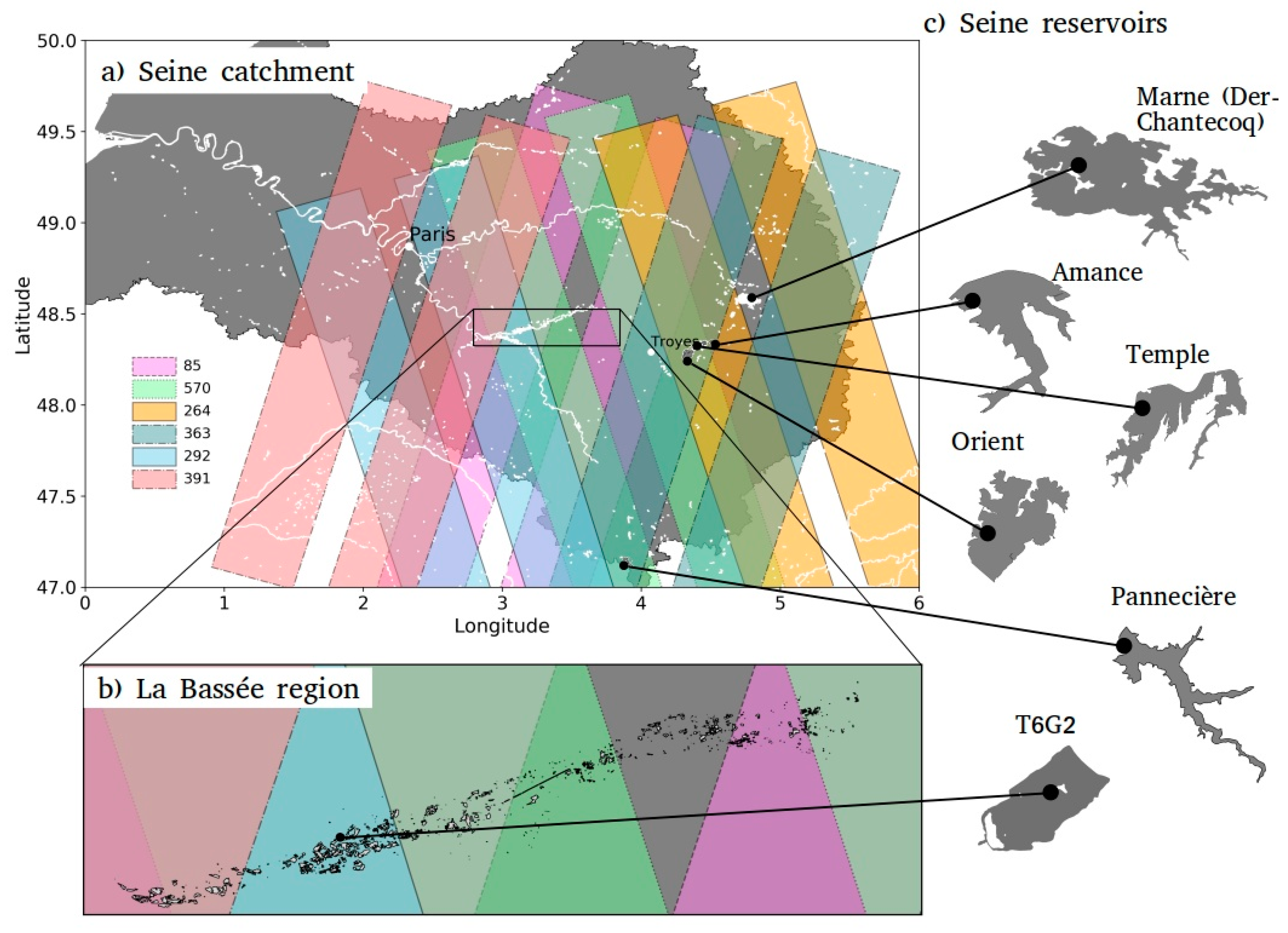
2. Study Region and SWOT Coverage

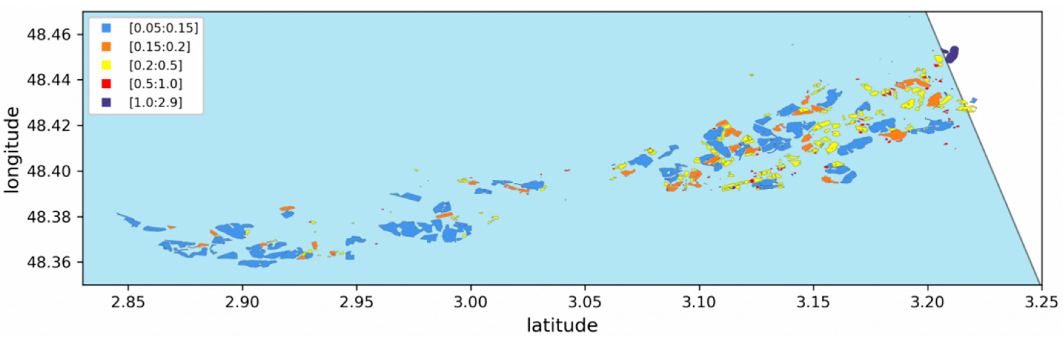
2.1. Seine Reservoirs and La Bassée Gravel Pits

The study region, the location of the Seine reservoirs and La Bassée gravel pits considered in the following are presented in Figure 1. Table 1 lists the reservoirs name, surface area, water holding capacity and maximal depth.
We focus here on the upstream part of the Seine river, which is one of the major rivers of France (777 km long), flowing through the city of Paris into the English Channel and draining a basin of about 79,000 km2. The river is regulated for discharge control (reducing flood peaks and holding water levels during low-flow periods), with five reservoirs built on the main stream and tributaries (the Marne, Yonne and Aube rivers) managed by the Seine Grands Lacs basin authority. Among these hydraulic structures, the oldest one is the Pannecière dam, built on the Yonne tributary and commissioned in 1949, which covers an area of 5.2 km2, with a maximum water holding capacity of 80 Mm3 and a maximum depth of 49 m. The four other structures are all diversion reservoirs connected to the Seine, the Marne and the Aube rivers, which operate in the following way: the water is removed from the river by diversion in winter and spring, to fill the reservoir and reduce the floods downstream; storage is released to the river during summer and early fall to maintain water levels and hold the production of drinking water and water needs for crops irrigation [22,23]. Their surface area varies from 5 km2 (Amance on the Aube river, which is the smallest, with a water holding capacity of 22 Mm3) to 48 km2 (Der-Chantecoq on the Marne river, which is the largest, with a holding capacity of 349 Mm3).
In between the confluences of the Aube-Seine and Yonne-Seine rivers, the La Bassée alluvial plain is a regularly flooded section of the Seine river of about 364 km2 (about 70 km long and 5 km wide) connected to a chalk aquifer characterized by the presence of numerous gravel pits (about thousand identified, among which more than 530 present a surface area less than 1 ha). Some of them are monitored, such as the gravel pit “T6G2” equipped with thermal and water pressure instruments (A. Jost, personal communication). These instruments are designed to monitor the water level and temperature, in order to better understand the water transfers between the chalk and alluvial aquifers and the gravel pit.

2.2. SWOT Mission and Orbits

SWOT will be equipped with a Ka-band (35.75 GHz or 8.6 mm wavelength) SAR interferometer instrument (called KaRIn) with near nadir incidence angles (between 0.6° and 3.9°), which will provide measurements of water surface elevation over ocean and continental surfaces with a pixel resolution of 6 m in the along-track direction and 10 m to 60 m from near range to far range in the across-track direction, depending on the location within the two 50-km wide swaths provided by the two antennas on each side of the satellite with a 20 km gap in between [15]. On continental surfaces, SWOT will allow to measure water level changes for wetlands, lakes and reservoirs larger than 250 × 250 m2 with a repeat cycle of 21 days. However, because of the swath coverage and the orbit characteristics, the number of observations per cycle will vary according to the latitude. For our studied reservoirs and gravel pits, the number of revisits can be up to four observations within 21 days, with time gaps ranging from 4 to 17 days within this revisit cycle.
The days of observation per revisit period are listed for all the reservoirs and the La Bassée region, in Table 1. As an example, Figure 1 shows the sampling area of all the orbits which will intersect the Seine reservoirs and the La Bassée alluvial plain. Unfortunately, one reservoir (Marne-Der-Chantecoq) within the Marne watershed, located at the intersection of the nadir gap areas, will never be observed by the SWOT-KaRIn instrument. Nevertheless, six SWOT orbits will sample the studied area (85, 264, 292, 363, 391 and 570) and their respective swath is visualized in Figure 1 (note that the color code associated to each orbit will be the same hereafter). The Orient and Temple reservoirs will be sampled three times over the 21-day cycle repeat orbit pass, at 9-, 13- and 20-day regular intervals by the orbits 264, 363 and 570. The Amance and Pannecière reservoirs will be sampled twice at 9-, 13- (respectively, 13-, 20-) day intervals at orbits 264 and 363 (respectively, 363, 570). The La Bassée region will be sampled up to four times at 3-, 10-, 14- and 20-day intervals at orbits 85, 292, 391 and 570.

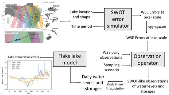
3. Lake Model and SWOT Simulator

3.1. FLake Lake Model

The FLake lake model [24] was chosen to assess the potential contribution of the near future SWOT data to the monitoring of the energy budgets of the water bodies of the Seine basin for environmental studies. FLake is a one-dimensional (1D) model dedicated to the simulation of the surface-atmosphere energy transfers and principally designed to be coupled to weather prediction or climate modeling. The model considers two layers in the lake: a top mixed layer with uniform vertical temperature and a thermocline below, parameterized according to a self-similarity concept. A sediment layer can be optionally added at the bottom, based on the same concept. Freezing processes and evolution of a snowpack layer above the ice layer are also simulated with a bulk approach, and a parametric representation of the temperature profile. The model is already implemented in many numerical weather prediction and climate models [25,26,27] to cite but a few, and was chosen to represent water surfaces in the ORCHIDEE land surface model, the continental part of the Institut Pierre Simon Laplace (IPSL) climate model [28].
Two energy budgets (for the mixed layer and for the bulk lake) are calculated to solve the temperature profile and calculate the energy surface fluxes (radiative and turbulent fluxes) at the lake-atmosphere interface, given the atmospheric forcing (incoming solar and atmospheric radiations, air temperature and humidity and wind speed). In order to characterize the thermal and radiative properties of the lake, four main parameters need to be prescribed: the lake depth, the water surface albedo, the light extinction coefficient and the wind fetch. A preliminary study [28] quantified the respective sensitivity of the model outputs to these four parameters. It confirmed the key role of lake depth on the simulation of the surface temperature and fluxes, and therefore, the expected contribution of SWOT instrument for improving the model predictions.

3.2. SWOT Simulator

The SWOT large scale simulator [21] developed by CNES was used here to generate the water surface elevation (WSE) errors on the studied water bodies. The simulator is composed of two parts: one module to simulate the satellite orbitography and the instrument swaths given the characteristics of the mission (therefore, the revisit times and the geometric configuration), and a second module to calculate the final error budget of the SWOT measure at the pixel level. The simulator accounts for the two main sources of error that will affect the KaRIn measurements, i.e., the random errors corresponding to the instrument thermal noise and geometric signal decorrelation and the systematic errors linked mostly to tropospheric propagation delay and rolling errors. The random errors are generated at pixel level and can be approximated as white noises with normal distribution and standard deviations varying with the pixel location in the swath. Unlike the instrumental noise, the systematic errors are constant in the swath for a given time. They are modeled for each date as random variables in this version of the simulator. Here, the systematic errors are generated with Gaussian white noise with a standard deviation equal to 0.05 m. Gaussian white noise is also used to generate the instrumental errors, with a standard deviation varying around 3 m for viewing angle less than 3° and increasing up to 30 m for larger values. Thanks to the random nature of the signal and the large number of measurements within the studied lakes, the instrument budget error may be largely reduced by averaging over a number of pixels and then dividing by the square root of this number [29,30]. It should be noted that the topographic and vegetation layover are not accounted for in this simplified simulator, but a geolocation error due to the interferometric baseline roll angle can be estimated. It has been activated here in the water surface elevation (WSE) error simulations. Additionally, dark water pixels corresponding to the case of specular water reflectivity were not accounted for in the simulations. More information on the main features of the large-scale simulator can be found in [21].

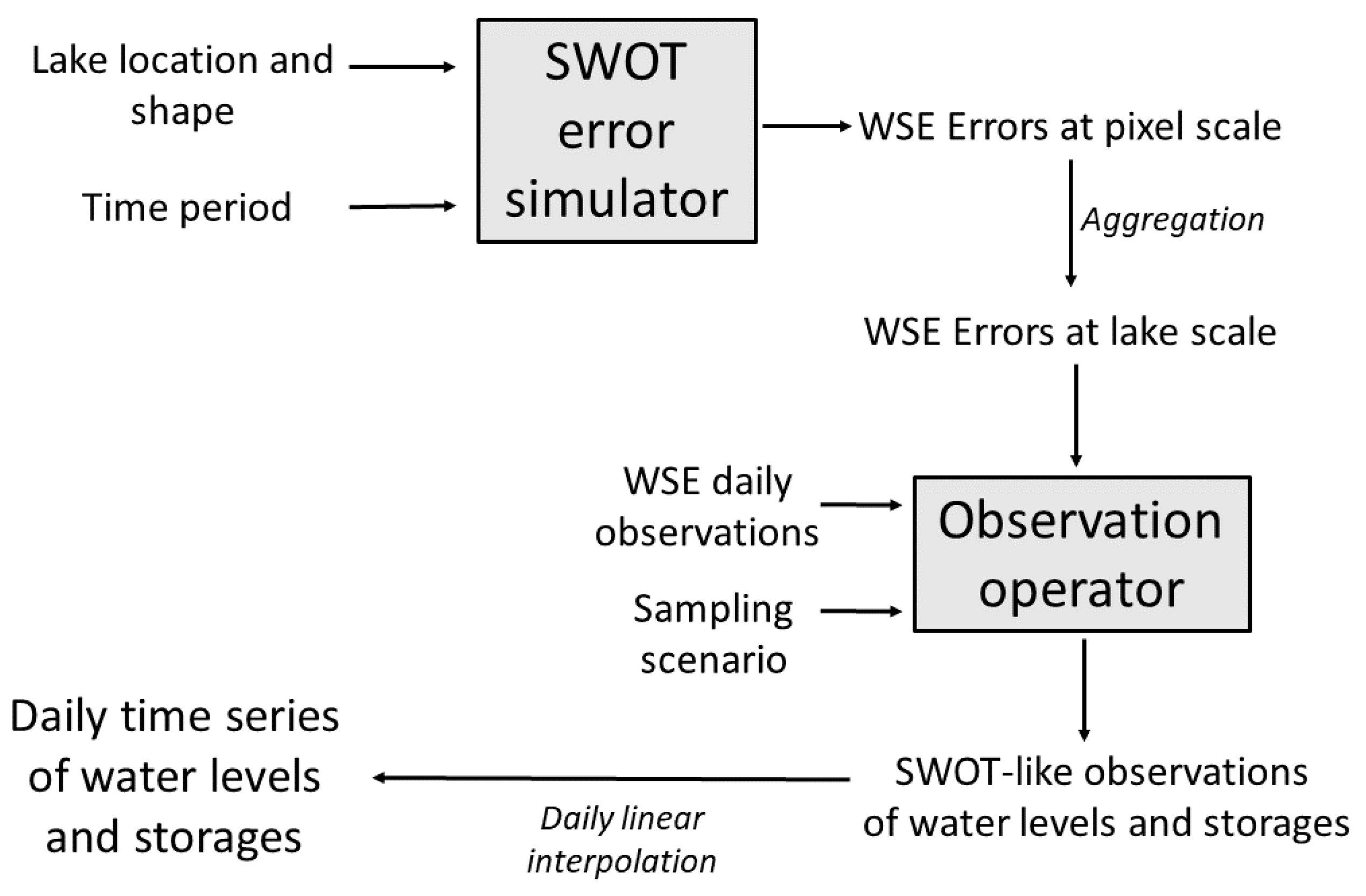
4. Simulation of SWOT-Like WSE Errors

4.1. Method

WSE errors were simulated with the large-scale SWOT simulator on the studied Seine reservoirs and La Bassée gravel pits. The contours of these water bodies as georeferenced polygons were extracted from the CARTHAGE database (French national hydraulic database BD CARTHAGE® IGN; see www.sandre.eaufrance.fr/Referentiel-hydrographique) and redrawn from the 2014 ortho-photography database (BD ORTHO® IGN). The simulations were performed for a five-year period to mimic the expected lifetime of the satellite set as a goal [16]. We analyzed the WSE errors at the pixel scale and at the lake scale after averaging the random errors on our studied water bodies. The spatial and temporal variations are analyzed according to the satellite orbit for the four Seine reservoirs and 1062 gravel pits of La Bassée region.

4.2. Results

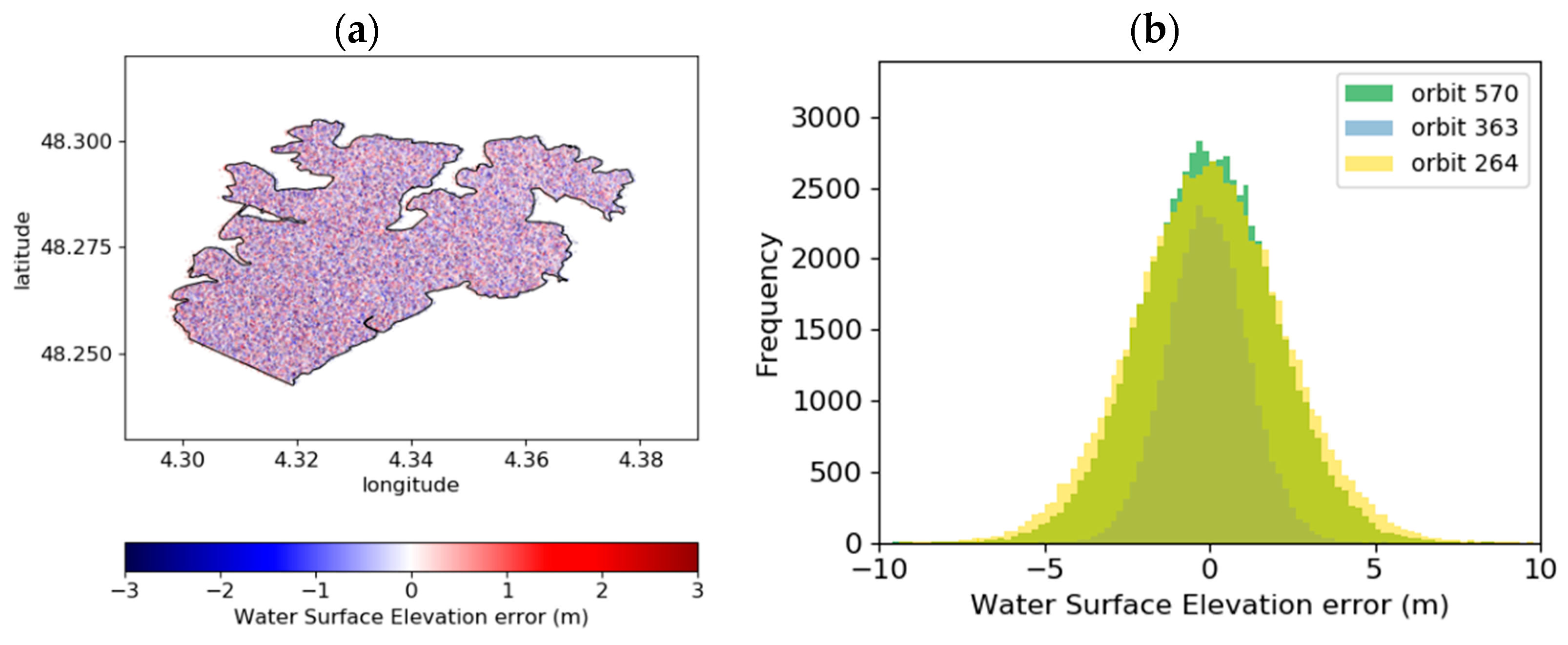
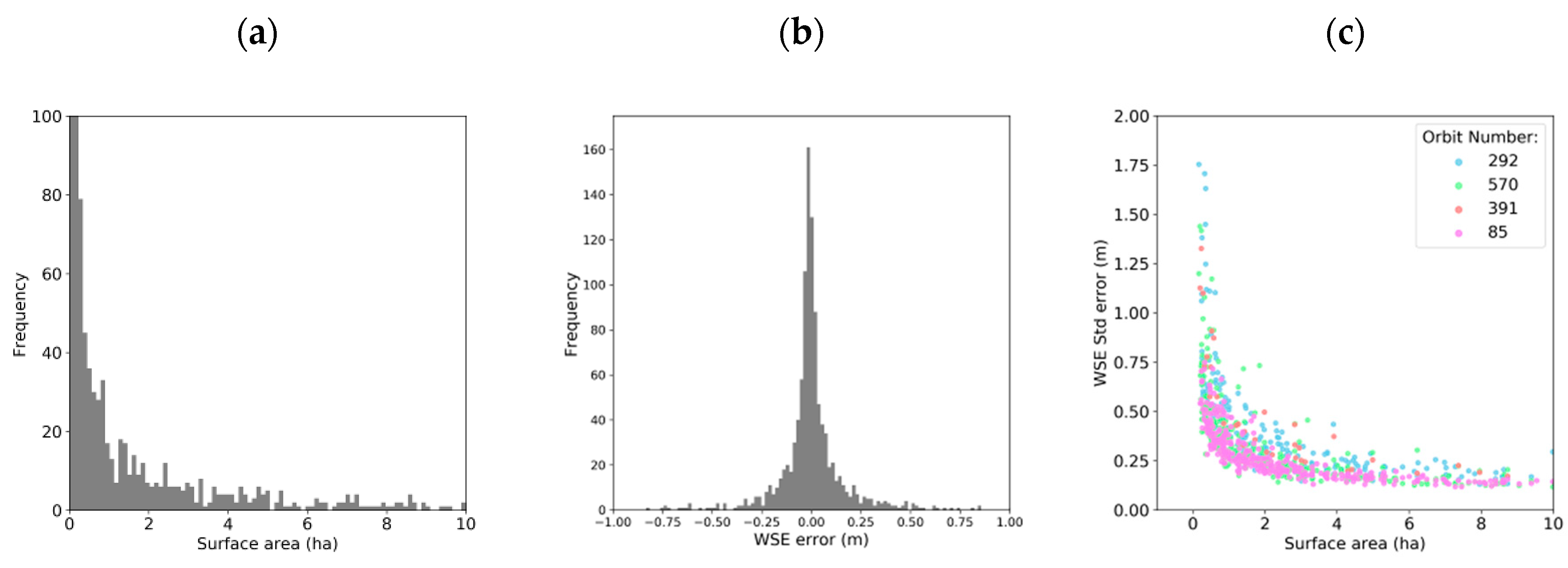
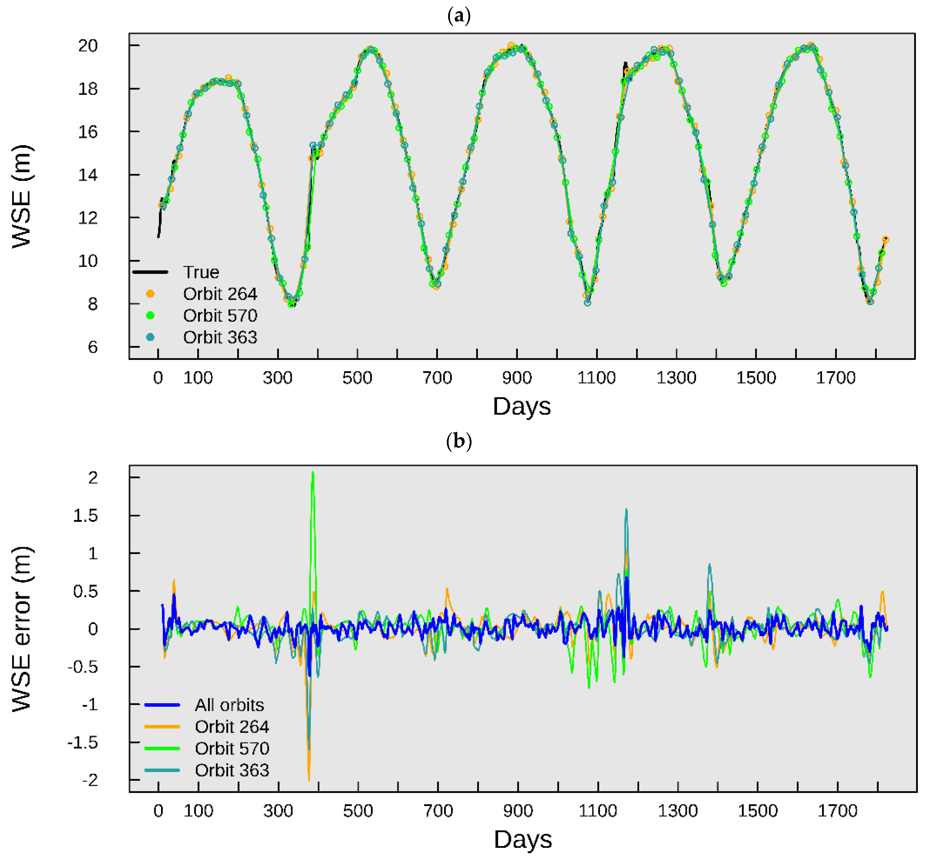
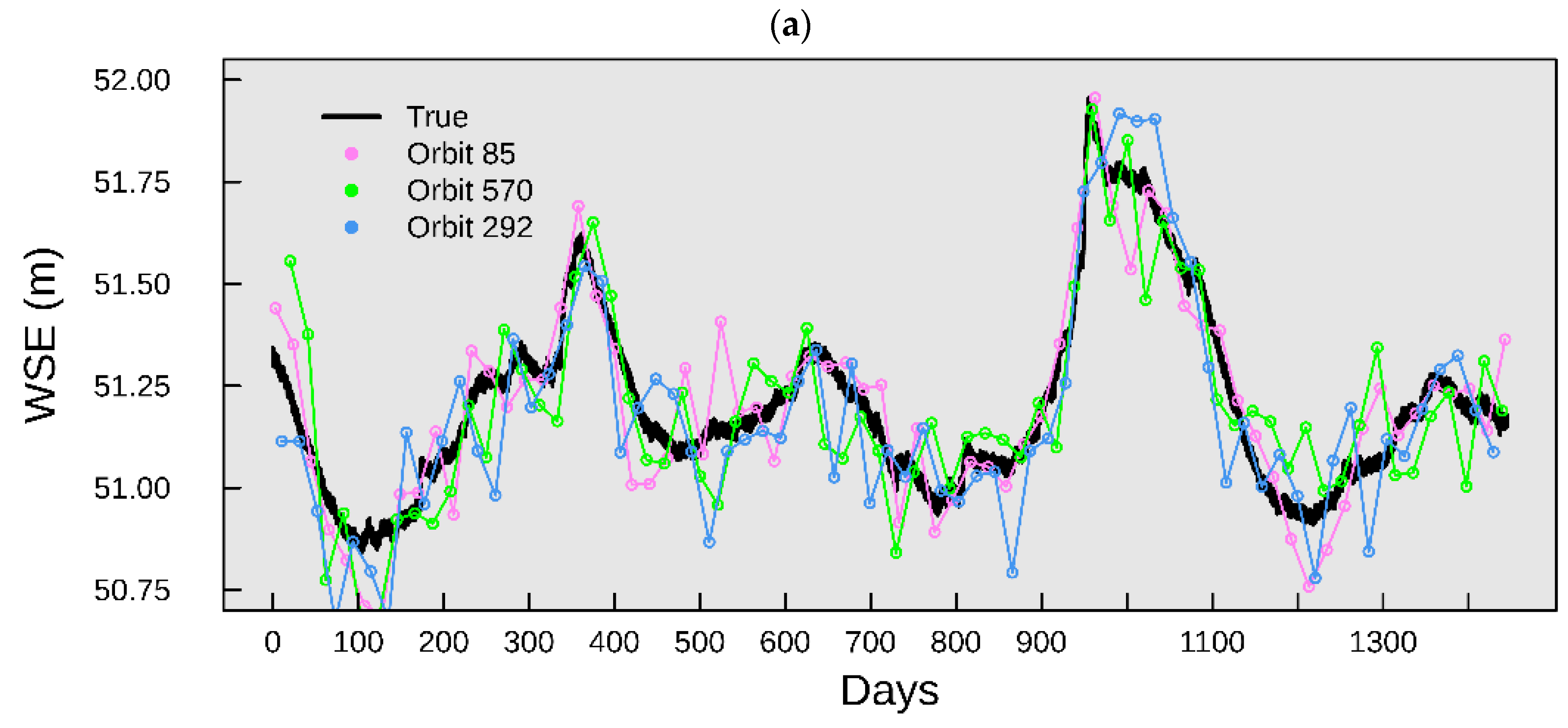
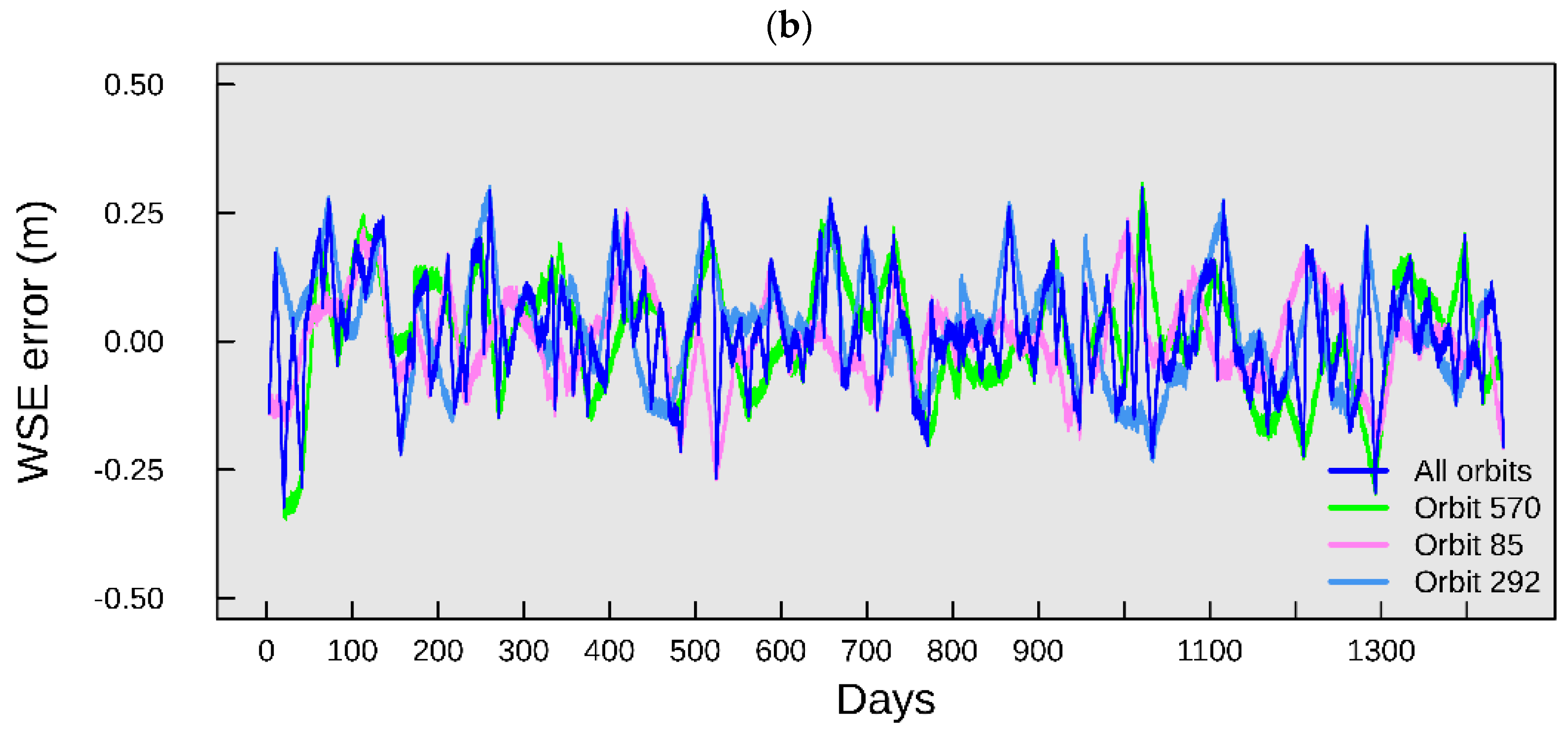
4.2.1. WSE Errors on the Seine Reservoirs

Pixel-Scale WSE Error

Figure 2 presents an example of the pixel cloud obtained for one pass (orbit 264, day 9 of the simulation) over the Orient reservoir. The noisy nature of the signal is clearly seen with pixel error values ranging between −10.09 m and +10.03 m, leading to a mean error value equal to −0.024 m. The effect of the geolocation error is clearly seen on the western part of the reservoir with larger positive errors. This can be explained by the fact that the geolocation error impacts differently positive and negative vertical errors, in such a way that positive errors will be moved away from the satellite track and the other way round for negative errors. The distribution of the errors calculated over the five-year simulation (Figure 2b) shows the lowest range of variation for the orbit 363 compared to the orbits 570 and 264 (presenting the largest errors). This is an illustration of the impact of the distance of the Orient reservoir to the nadir line, which is roughly 20 km, 45 km and 47.5 km for the orbits 363, 570 and 264, respectively (see Figure 1). Therefore, the viewing angle is indeed lower for the orbit 363, explaining that the errors range only between −5.34 m and +4.85 m, in this case.

Lake-Scale WSE Error

When averaged over the lake surface area and because of the random nature of the signal, the pixel errors compensate and the mean WSE error (as it will be observed by the SWOT-KaRin instrument at the lake scale) decreases drastically down to a few centimeters. The standard deviation (std) and maximal (absolute value) WSE errors calculated over the five-year simulation period (90 cycles) are summarized in Table 2 for the four reservoirs and the instrumented gravel pit of La Bassée (T6G2). The surface extent and the average number of SWOT-like measurements (Np) for each orbit configuration are also provided. Note that Np can vary slightly from one pass to the other, due to the geolocation error. It can be seen that for all the lakes, the standard errors are very small, and up to 0.11 m for the smallest water body (T6G2). The maximum errors are of a few tens of centimeters and up to 0.32 m for the Pannecière reservoir and T6G2 gravel pit. The location of the water body inside the swath has a limited impact. The lower the incidence angle, the lower the error, as shown for example by the difference of about 20% between the errors obtained for the Orient reservoir for the Orbit 264 and those obtained for the Amance reservoir. In summary, these simulations clearly show that the studied water bodies are large enough to allow the measurement of their depth with a decimetric precision, even for a small lake of about 20 ha as the gravel pit T6G2.

4.2.2. WSE Errors on La Bassée Gravel Pits

In the region of La Bassée, 1062 gravel pits were extracted from the CARTHAGE database. Their size ranges between 35 m2 and 0.9 km2 (90 ha) and the size distribution presented in Figure 3a clearly shows the dominance of the small gravel pits with size lower than 1 ha. The simulator has been run on all the gravel pits sampled by the four orbits covering the region, i.e., on 801 water bodies, and on a five-year period. Given the 21-day orbit cycle, the number of observations over five years is therefore equal to 90.
The simulated SWOT-like errors averaged at the gravel pit scale are displayed on Figure 3b. The errors are larger than the ones simulated for the Seine reservoirs and range mostly in the [−1 m, +1 m] interval. Among all the errors simulated on the whole period (136,214 errors in total), around 18% are above 0.5 m (30% being lower than 0.1 m).
The impact of the size of the gravel pit on the standard deviation of the measurement error is clearly shown on the scatterplot presented in Figure 3c, where the smaller gravel pits show the largest standard deviation errors, up to 1.75 m. The four orbits show the same features with an exponential decrease to a value lower than 0.25 m when the surface area exceeds 4 ha. Among all, the orbit 85 presents the lowest values and the orbit 292 the largest. This can be explained by the location of the La Bassée region within the different swaths, with the orbit 85 observing the region with the lowest viewing angles (lowest distance to the nadir track). In any case, the results show that for the gravel pits that will be observed operationally by SWOT (with a size larger than 6 ha), the precision of WSE will be better than 0.25 m.
The spatial analysis of the WSE errors on the whole set of simulations did not show any correlation with the size of the gravel pit (Corr = −0.08), but some features appeared when the analysis was reduced to one orbit. As an illustration, Figure 4 presents the standard deviation of the errors calculated for all the gravel pits sampled by the orbit 292 located on the western part of the La Bassée region (including the T6G2 gravel pit), and calculated over the 90 SWOT-like observations of the five-year study period. Indeed, the plot shows larger values for the smaller lakes and larger values when moving from west to east, i.e., moving to the far edge of the swath. The largest gravel pits show standard values lower than 0.15 m, which is the order of magnitude obtained for T6G2 (Table 2). Moreover, most of the gravel pits (70%) present standard values lower than 0.5 m and only 11% show values larger than 1 m. The largest value (2.83 m) is obtained for a gravel pit that is located on the border of the swath and is strongly affected by geolocation errors.

4.2.3. Contribution of SWOT in WSE Daily Monitoring

Given the expected SWOT WSE errors, we found it interesting to assess the impacts of these errors on the daily monitoring of our studied water bodies according to the period of revisit, in order to quantify the benefit of SWOT temporal sampling on the reconstruction of daily records of both WSE and water volumes.
  • Methodology
For this purpose, we have generated, for each of the Seine reservoirs, SWOT-like observations of surface water level by adding the simulated errors to in-situ observations provided by the Seine Grands Lacs basin authority over the period 2003–2007 at daily time step. It should be noted that these data are water levels provided by in-situ probes or observers. These pseudo-observations were linearly interpolated at a daily time step, to generate daily time series of surface water levels as they could be derived from SWOT observations. The corresponding water volumes were estimated using empirical relationship between water storage and water level, calibrated on each lake with actual observations as proposed by [31]. In order to assess the impact of temporal sampling on the WSE errors, we generated different daily time series corresponding to different sampling scenarios, considering either a single measurement over the 21-day cycle period with each orbit separately or all the possible measurements (two or three depending on the reservoir studied). The latter scenario will be called “All orbits” hereafter. The developed methodology is displayed in Figure 5.
  • Results
As an example, Figure 6a shows the daily variation of WSE as it could be derived from SWOT observations on the Orient lake on a five-year period considering the three orbits covering the lake, therefore, for four sampling scenarios (each of the three orbits individually and all jointly). The true observations are plotted on the same graph as a reference. The WSE errors calculated as the differences between the daily time series and the true observations for the four sampling scenarios, are plotted on Figure 6b. The benefit of the more frequent sampling is clearly seen with a significant reduction of the errors when all the orbits are considered jointly (std = 0.1 m). In comparison, the errors are two to four times larger when a single orbit is considered. As expected, the errors are larger in winter, when the temporal variations of the reservoir volumes are the largest, because of the management operations (water released to river to empty the reservoirs before the floods and then stored from November on). During these periods, the WSE anomalies can reach several meters, like in winter 2003–2004 (Year 2 of the simulation, Figure 6b), when it goes up to 2 m in the case where only orbit 570 or orbit 264 is used to follow water level.
Table 3 summarizes the values of the maximal errors and standard deviations of the WSE errors, calculated for the four reservoirs on a five-year period. The largest error is found for the Orient lake and orbit 570 (WSE error of 2.08 m, corresponding to a storage error of 4.6 Mm3). In all cases, the errors are lower when all the observations are used to monitor the water level and storage, but the reduction of error is larger for the Orient and Temple reservoirs compared to the Pannecière and Amance ones. Indeed, the error is reduced by a factor of three for the first two reservoirs and by only 40% and 20% for Pannecière and Amance, respectively. This result can be easily explained by the more frequent sampling of Orient and Temple compared to the other two reservoirs (three observations/cycle instead of two). It shows that the improvement increases with the number of revisits, and also that two observations well distributed in the 21-day interval (Pannecière case) are better than when they are clustered (Amance case), especially during filling/emptying time periods when the WSE varies rapidly.
The same analysis has been performed for the monitored gravel pit T6G2, for which four years of measurements of water elevation above sea level are available on the period 13 May 2015–12 June 2019. As an indication, the elevation of the surrounding area is around 53 m. In the case of an unmanaged lake, the WSE temporal variations (Figure 7a) are much smoother than those for the managed reservoirs previously described. Therefore, the daily maximal and standard errors are much smaller (up to a factor of seven for the maximal error and a factor of two for the standard error) and the benefit of increased sampling is less significant (Figure 7b and Table 3). The anomalies show about the same patterns whatever the sampling scenario. The maximum error is equal to 0.35 m with a standard deviation of 0.11 m (in the case of orbit 570) with no reduction when all orbits are used. This result would suggest that for such small water bodies, the SWOT error is too large and cannot be reduced by an increase of the sampling up to three observations per cycle; a larger sampling would be needed in that case.

5. Impacts on Water Energy Budget Modeling

The contribution of SWOT data on the estimation of the energy budget of the Seine reservoirs and gravel pits has been assessed through sensitivity experiments performed with the FLake lake model [24]. As demonstrated by [28] through a global sensitivity analysis, lake depth plays a key role in the calculation of lake temperature and heat fluxes, and consequently, in the assessment of lake evaporation. In order to quantify the added value of SWOT measurements on the monitoring of these surface variables, we have designed a set of modeling experiments on our studied water bodies, corresponding to various levels of knowledge of the key depth parameter. The study was performed on the four Seine reservoirs as well as on the T6G2 gravel pit.

5.1. FLake Simulation Experiment Design

Three depth scenarios were built to quantify the contribution of SWOT data on surface temperature and heat fluxes modeling:
  • The first scenario (called REF) considers that the actual depth of the reservoir/gravel pit is known precisely and provided by daily local measurements; FLake simulations forced by such true data will serve as reference.
  • In the second scenario (called MAX), the water level is not measured but the maximal capacity of the reservoir/gravel pit is known (as given by the literature) and will be used to prescribe a constant value to the depth parameter.
  • In the third scenario (called SWOT), the water depth is regularly measured from space (and prone to errors) and updated at the SWOT sampling rate considering all the orbits covering the lake. It is assumed here that the water depths will have be derived from the water surface elevation measured by SWOT provided a reference measurement.
For these three scenarios, we generated depth time series for the five Seine water bodies (four reservoirs and T6G2 gravel pit) on the two time periods previously studied (2003–2007 for the reservoirs and 2015–2019 for T6G2). All the simulations were performed using the same atmospheric conditions (incident radiation, air temperature and humidity, wind speed) based on atmospheric reanalysis provided by the WFDEI (WATCH Forcing Data methodology applied to ECMWF Re-Analysis-Interim) database [32]. In order to isolate the contribution of a better knowledge of the lake depth, all the other parameters prescribed in FLake were kept the same, equal to the standard values proposed by [24] and available at http://www.flake.igb-berlin.de. It should be noted that the sediment module of FLake was not used in these simulations and that for all the simulations, a three-year spin-up period was performed to reach model equilibrium and get rid of incorrect initialization states. The results are discussed in terms of surface temperature (TS) and latent (HL) and sensible (HS) heat fluxes, which are the main lake variables interacting with the atmosphere above.

5.2. Modeling Results

The FLake simulations based on the MAX and SWOT scenarios were compared to the one forced with true depth values (scenario REF). The differences can be interpreted as errors propagated from the depth errors to the surface temperature and fluxes of the studied lakes.

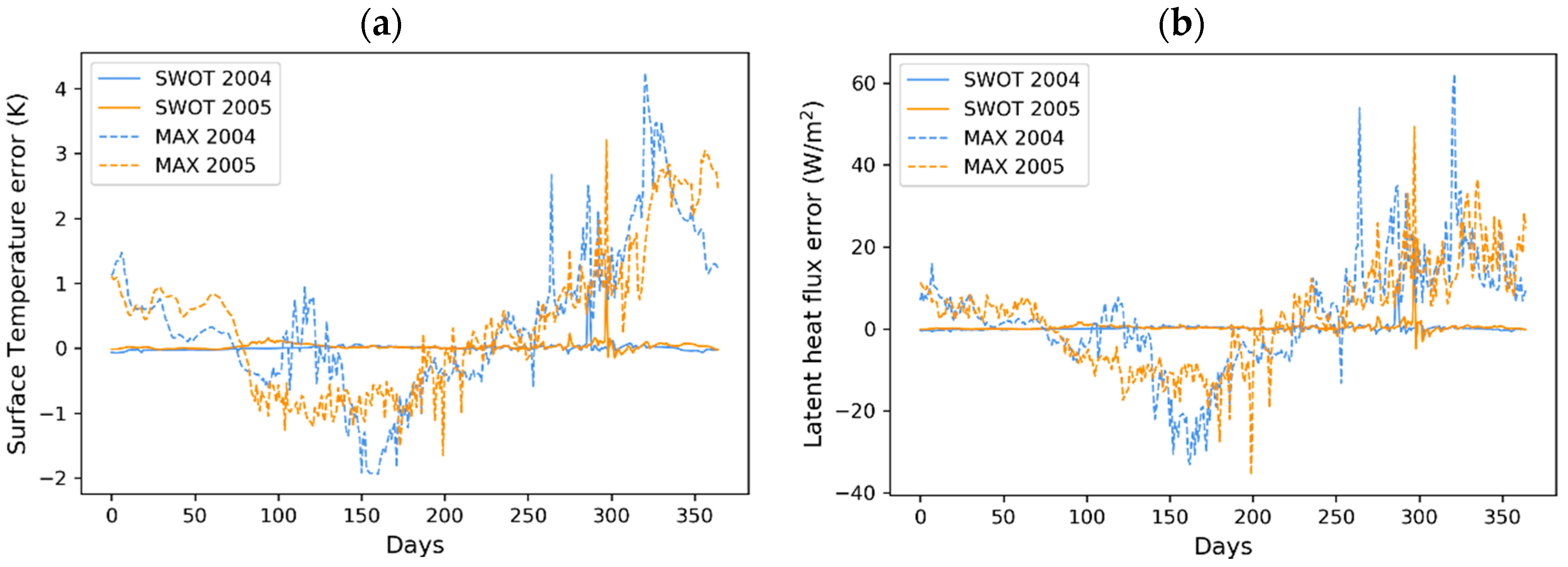
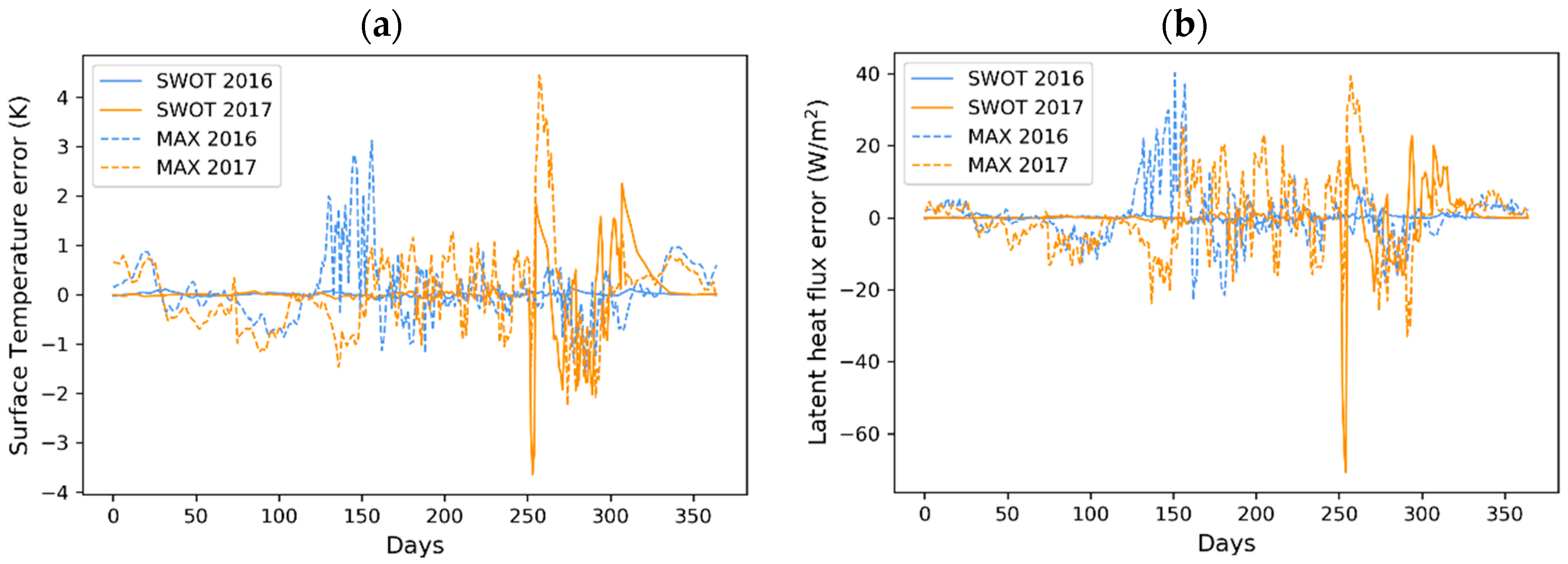
5.2.1. Model Errors on Seine Reservoirs

The analysis was performed on the four studied reservoirs and is summarized in Table 4, in terms of maximal and standard deviation errors. Figure 8 shows the daily surface temperature and evaporation flux errors obtained on the Orient reservoir on two years, 2004 and 2005, for the SWOT and MAX scenarios.
The plots clearly show the strong reduction of the errors in the SWOT simulations, on TS and also HL. The systematic overestimation of TS in winter season and underestimation in summer is the result of the overestimation of the reservoir depth by the MAX scenario (larger in winter, as discussed previously) compared to the true values, as shown in Figure 6a. Such depth errors, which can be up to 17 m at the end of fall in the case of the Orient lake, can drastically modify the lake regime, the convection flows and the temperature profile. Indeed, the largest errors occur during the periods when the reservoir level is minimum at the end of fall and in summer when the atmospheric demand is the largest, depth errors having much lower impacts in winter, when the potential evaporation is low. Here, during these two years, TS errors can exceed 4 K, which translate in HL errors up to 60 W/m2, namely an evaporation error of 2.5 mm/day. In the SWOT scenario, the depth errors are substantially reduced with maximum values up to 0.68 m (see Table 3), which will lead to TS and HL errors less than 1 K and 10 W/m2, respectively.
Table 4 summarizes the results obtained for the four reservoirs, and shows the benefit of the SWOT future observations on the reservoir energy budget monitoring. Maximal and standard deviation errors are reduced in all cases. The standard errors as compared to the MAX scenario are reduced by a factor of 6 for the Orient lake and up to 10 in the case of the Amance lake, which is the one presenting the largest error in the MAX scenario. The fluxes errors (latent heat HL and sensible heat HS fluxes) are reduced by the same factors as expected.

5.2.2. Model Errors on T6G2 Gravel Pit

On the much shallower T6G2 gravel pit, whose depth spatially varies up to 6 m, the SWOT contribution to the reduction of energy budget errors is also significant. Figure 9 presents the TS and HL errors obtained for the two scenarios MAX and SWOT, simulated for the years 2016 and 2017 (for which the depth records cover the whole year). In this case, the depth translated errors are larger than for the deeper reservoirs, for at least two reasons: the depth errors are larger and the sensitivity of the energy budgets components to the depth parameter is larger for shallow lakes, as shown by [28]. The errors are dominant in spring and fall, which correspond to the two annual periods of lake mixing and the disappearance of the thermocline layer. The date of this turnover period is strongly dependent on the lake depth: a positive/negative error on the depth will lead to a time difference (delay/ahead, respectively) in the mixing process. Interestingly, these periods are well simulated both in 2016 and in spring 2017 in the SWOT scenario, whereas, in 2017, the fall turnover after DOY 250 seems to be delayed by a few days in both simulations MAX and SWOT. This is explained when looking to the SWOT errors simulated on the same period, which happened to overestimate the WSE of the gravel pit (see Figure 7a, around day 980), and consequently, lead to a delay of the lake turnover and an overestimation of TS (since the temperature of the surface layer is larger than the bottom temperature at the end of summer). The larger magnitude of the SWOT errors on this small water body does not allow to monitor precisely this specific event. The errors statistics on the four-year period summarized in Table 4 highlight again the added value of the SWOT observations even for this small lake, with a reduction of the standard deviation of the errors by a factor of around two as compared to the MAX scenario, both on surface temperature and fluxes.

6. Discussion

6.1. SWOT Reduction of Errors

The SWOT mission will provide, in a very near future, surface elevation of water bodies with an unrivalled decimetric precision and with a repeat cycle of 21 days as a minimum. These new observations will help monitoring surface water fluxes and storages in rivers, lakes, reservoirs and wetlands. In this study, we focused on the Seine basin and its large reservoirs and alluvial plain upstream the city of Paris, and tried to assess the future contribution of these new observations to follow water levels but also surface fluxes through a lake energy budget model.
The large-scale simulator [21] was used to characterize the expected instrument errors on the studied water bodies. Based on the satellite orbit and swath characteristics, the sample rates and days of revisit were computed over four out of the five Seine reservoirs, (one of the reservoirs will unfortunately never be observed because of the instrument observation nadir gap) and 801 gravel pits of the alluvial plain. Some of the gravel pits will be sampled up to four times within the 21-day orbit cycle, which will provide measurements at time intervals lower than 6 days. The SWOT simulator results show that the expected measurements over the large reservoirs will be obtained with a precision around 0.10 m and up to 0.25 m for the smaller gravel pits with size down to 6 ha. These results are in line with the instrument budget errors [29] and demonstrate the tremendous interest of SWOT future data for water management purposes, especially for poorly gauged and ungauged reservoirs and lakes. They are also in agreement with the previous works of [18,19,20] based on the JPL-SWOTsim simulator, even though our errors appear slightly larger. Thus, the Agoufou lake in Sahel, with an area varying from 100 ha to 250 ha, [20] showed that WSE could be retrieved with an accuracy better than 4 cm.
These errors were used in a second step to quantify water levels and storages errors in an objective of daily monitoring, using all the SWOT observations potentially available. Daily time series were generated by linear interpolation of SWOT observations and were compared to true measurements, in order to assess the potential of SWOT for the daily monitoring of the Seine reservoirs. The results show a slight degradation of the WSE estimation with large errors up to 2 m, occurring when only one measurement in the 21-day interval is available and during the periods of filling/emptying of the reservoirs when the water level can change very rapidly. Fortunately, these errors are considerably reduced if the reservoir is sampled more frequently. In the case of the Orient reservoir, the errors are reduced by a factor of up to 3 when the three observations within the 21-day period are used. For smaller and unmanaged water bodies such as the Seine gravel pits, the error degradation linked to the linear interpolation is less significant and the benefit of frequent revisit compared to only one was not demonstrated, because of the smoother variations of WSE and the larger errors, which would benefit from a more frequent revisit.
Finally, the time series of WSE were used in the FLake model to assess the contribution of SWOT for lake energy budget modeling. In such models, the lake water level or mean depth is a very sensitive parameter, because it determines key processes such as the flow convection within the lake due to the water density gradients, which further affects the seasonal thermal stratification. In order to quantify the foreseen added value of SWOT, we generated SWOT-like time series of daily lake depth by direct assimilation of SWOT-like observations and used them to drive the FLake model. The results were compared to Flake simulations performed either with true daily observations of depth or using a constant value. The analysis highlighted the benefit of the SWOT observations for the modeling of surface water temperature and fluxes with, again, major error reductions. Therefore, this confirms the importance for developing tools and models to prepare the assimilation of the future SWOT products in catchment monitoring systems.

6.2. SWOT Perspectives for Reservoir Monitoring

This study was limited to a small number of water bodies, but their diversity, from the small gravel pit to the large reservoir, provided insights on the future SWOT errors on such water bodies (managed and unmanaged). Furthermore, we addressed how these errors translate into surface temperature and flux errors in a lake energy budget modeling. The next step will be to use the SWOT data to also control the mass budget, through the assimilation of both the surface extent and level changes, or the use of the future SWOT products of lake water storage change, as shown by [33]. We anticipate that the use of such data will bring lake modeling major steps forward. Moreover, if we consider the added value of the future discharge products, it can be expected that the SWOT mission will bring new and very valuable data for hydrology.
The characterization of the SWOT errors was investigated using the large-scale simulator, which integrates the various types of errors expected after launch of the mission. In the simulation, the lake contour (and therefore its size) was kept constant. This assumption should not have impacted our error estimations on the Seine reservoirs because of their large size. It should be the same for most of the gravel pits whose size changes little during the year. Nevertheless, it will be interesting in the following, to run the JPL simulator on our studied water bodies to quantify the simulator uncertainties and also to test the last version of the large-scale simulator, which include some new features, such as spatialized tropospheric errors and improved rolling errors.
SWOT future lake products will include both water extent and water levels. The seasonal dynamics of water extent will also be a valuable information to better constrain lake and hydrological models. The global capacity of the instrument will allow to provide these data at global scale. Such information will be very useful to better assess the role of water bodies and wetlands on the global water cycle and more generally the land–atmosphere feedback for environmental and climate studies.

7. Conclusions

We used the CNES large scale SWOT simulator to simulate the expected instrument errors over the Seine reservoirs and gravel pits of its alluvial plain, in order to assess the potential of these new data to be used in the daily monitoring of water levels and storages. The pseudo-observations generated were used, firstly, to explore how SWOT will observe the studied reservoirs and the expected uncertainties, and secondly, to quantify the resulting surface temperature and fluxes errors in lake energy budget modelling.
Applied to four large reservoirs (with area varying from 5 km2 to 23 km2) and 801 gravel pits of various sizes (areas varying from 35 m2 to 0.9 km2), the simulator was used to estimate the expected precision of the future SWOT data (around 0.1 m for the reservoirs and better than 0.25 m for the smaller gravel pits). It was also used to provide the first quantitative assessment of the contribution of these data for constraining the simulation of the surface water energy budgets.
These findings confirm how valuable space altimetry is for reservoir/lakes monitoring, especially for ungauged water bodies or to complement in situ networks. The global capacity of SWOT to observe both water levels and surface extent and its increased spatial resolution and measurement precision, compared to the present instruments, will definitely help to better understand and model lakes and reservoirs dynamics. These new observations will certainly improve our knowledge about the role of water bodies on regional water and energy budgets, their impacts on the main biogeochemical cycles and their fate in global change scenarios.

Author Contributions

Conceptualization, C.O.; Methodology, C.O. and S.B.; Software, S.B., D.D., C.P. (Claire Pottier), and A.B.; Formal Analysis, C.O.; Resources, C.O., C.P. (Charles Perrin) and A.J.; Writing—Original Draft Preparation, C.O.; Writing—Review and Editing, C.O., A.B., S.B., A.J., D.D., C.P. (Charles Perrin) and A.d.L.; Visualization, T.V., A.B., K.P. and Z.Y.; Supervision, C.O.; Project Administration, C.O.; Funding Acquisition, C.O., C.P. (Charles Perrin), N.F., A.R. and A.J. All authors have read and agreed to the published version of the manuscript.

Funding

This research was funded by the French Space Agency (Centre National d’Etudes Spatiales) through the TOSCA-SPAWET program in preparation for the SWOT space mission. CEA (Commissariat de l’Energie Atomique et aux Energies Alternatives) is also acknowledged for funding part of A.B.’s PhD grant.

Acknowledgments

The Seine Grands Lacs basin authority is thanked for providing detailed data on the reservoirs of the Seine basin, as well as the French PIREN Seine program, who contributed to fund the data acquisition on the La Bassée gravel pits data. The anonymous reviewers are also acknowledged for their useful comments and suggestions on the previous version of this paper.

Conflicts of Interest

The authors declare no conflict of interest.

References

  1. Hanasaki, N.; Yoshikawa, S.; Pokhrel, Y.; Kanae, S. A global hydrological simulation to specify the sources of water used by humans. Hydrol. Earth Syst. Sci. 2018, 22, 789. [Google Scholar] [CrossRef] [Green Version]
  2. Wada, Y.; Wisser, D.; Bierkens, M.F.P. Global modeling of withdrawal, allocation and consumptive use of surface water and groundwater resources. Earth Syst. Dyn. 2014, 5, 15–40. [Google Scholar] [CrossRef] [Green Version]
  3. Verpoorter, C.; Kutser, T.; Seekell, D.A.; Tranvik, L.J. A global inventory of lakes based on high‐resolution satellite imagery. Geophys. Res. Lett. 2014, 41, 6396–6402. [Google Scholar] [CrossRef]
  4. Pekel, J.F.; Cottam, A.; Gorelick, N.; Belward, A.S. High-resolution mapping of global surface water and its long-term changes. Nature 2016, 540, 418–422. [Google Scholar] [CrossRef]
  5. Vorosmarty, C.J. The storage and aging of continental runoff in large reservoir systems of the world. Ambio 1997, 26, 210–219. [Google Scholar]
  6. Haddeland, I.; Heinke, J.; Biemans, H.; Eisner, S.; Flörke, M.; Hanasaki, N.; Stacke, T. Global water resources affected by human interventions and climate change. Proc. Natl. Acad. Sci. USA 2014, 111, 3251–3256. [Google Scholar] [CrossRef] [Green Version]
  7. Mao, Y.; Wang, K.; Liu, X.; Liu, C. Water storage in reservoirs built from 1997 to 2014 significantly altered the calculated evapotranspiration trends over China. J. Geophys. Res. Atmos. 2016, 121, 10097–10112. [Google Scholar] [CrossRef]
  8. Yin, Z.; Ottlé, C.; Ciais, P.; Zhou, F.; Wang, X.; Jan, P.; Dumas, P.; Peng, S.; Piao, S.; Li, L.; et al. Irrigation, damming and streamflow fluctuations of the Yellow River. Hydr. Earth Syst. Sci. Discuss. 2020, 1–28. [Google Scholar] [CrossRef] [Green Version]
  9. Sheng, Y.; Song, C.; Wang, J.; Lyons, E.A.; Knox, B.R.; Cox, J.S.; Gao, F. Representative lake water extent mapping at continental scales using multi-temporal Landsat-8 imagery. Remote Sens. Environ. 2016, 185, 129–141. [Google Scholar] [CrossRef] [Green Version]
  10. Calmant, S.; Seyler, F. Continental surface waters from satellite altimetry. Comptes Rendus Geosci. 2006, 338, 1113–1122. [Google Scholar] [CrossRef]
  11. Kouraev, A.V.; Zakharova, E.A.; Samain, O.; Mognard, N.M.; Cazenave, A. Ob’river discharge from TOPEX/Poseidon satellite altimetry (1992–2002). Remote Sens. Environ. 2004, 93, 238–245. [Google Scholar] [CrossRef] [Green Version]
  12. Frappart, F.; Seyler, F.; Martinez, J.M.; León, J.G.; Cazenave, A. Floodplain water storage in the Negro River basin estimated from microwave remote sensing of inundation area and water levels. Remote Sens. Environ. 2005, 99, 387–399. [Google Scholar] [CrossRef] [Green Version]
  13. Crétaux, J.-F.; Abarca-del-Río, R.; Bergé-Nguyen, M.; Arsen, A.; Drolon, V.; Clos, G.; Maisongrande, P. Lake volume monitoring from space. Surv. Geophys. 2016, 37, 269–305. [Google Scholar] [CrossRef] [Green Version]
  14. Crétaux, J.F.; Jelinski, W.; Calmant, S.; Kouraev, A.; Vuglinski, V.; Bergé-Nguyen, M.; Maisongrande, P. SOLS: A lake database to monitor in the Near Real Time water level and storage variations from remote sensing data. Adv. Space Res. 2011, 47, 1497–1507. [Google Scholar] [CrossRef]
  15. Biancamaria, S.; Lettenmaier, D.P.; Pavelsky, T.M. The SWOT mission and its capabilities for land hydrology. In Remote Sensing and Water Resources; Springer: Cham, Switzerland, 2016; pp. 117–147. [Google Scholar]
  16. Desai, S. Surface Water and Ocean Topography Mission (SWOT) Project, Science Requirements Document. NASA/JPL technical document D–61923; 2018. Available online: https://swot.jpl.nasa.gov/docs/D-61923_SRD_Rev_B_20181113.pdf (accessed on 31 March 2020).
  17. Peral, E.; Rodríguez, E.; Moller, D.; McAdams, M.; Johnson, M.; Andreadis, K.; Arumugan, D.; Williams, B. SWOT Simulator Quick User Guide; NASA: Washington, DC, USA, 2016; p. D-79123. [Google Scholar]
  18. Solander, K.; John, C.; Reager, T.; Famiglietti, J.S. How well will the Surface Water and Ocean Topography (SWOT) mission observe global reservoirs? Water Resour. Res. 2016, 52, 2123–2140. [Google Scholar] [CrossRef] [Green Version]
  19. Bonnema, M.; Hossain, F. Assessing the Potential of the Surface Water and Ocean Topography Mission for Reservoir Monitoring in the Mekong River Basin. Water Resour. Res. 2019, 55, 444–461. [Google Scholar] [CrossRef]
  20. Grippa, M.; Rouzies, C.; Biancamaria, S.; Blumstein, D.; Cretaux, J.; Gal, L.; Robert, E.; Gosset, M.; Kergoat, L. Potential of SWOT for Monitoring Water Volumes in Sahelian Ponds and Lakes. IEEE J. Sel. Top. Appl. Earth Obs. Remote Sens. 2019, 12, 2541–2549. [Google Scholar] [CrossRef]
  21. Desroches, D.; Pottier, C.; Blumstein, D.; Biancamaria, S.; Poughon, V.; Fjortoft, R. Large Scale Pixel Cloud Simulator and Hydrology Toolbox. In Proceedings of the SWOT Science Team Meeting, Montreal, QC, Canada, 23 June 2018. [Google Scholar]
  22. Villion, G. Rôle des lacs-réservoirs amont: Les grands lacs de Seine (The role of upstream dams: The large reservoirs of the Seine basin). La Houille Blanche 1997, 8, 51–56. [Google Scholar] [CrossRef] [Green Version]
  23. Rizzoli, J.L.; Gache, F.; Durand, P.Y.; Jost, C. Flood management in Ile de France, toward a shared and global strategy. La Houille Blanche-Revue Internationale de l’Eau 2011, 2, 5–13. [Google Scholar] [CrossRef]
  24. Mironov, D.V. Parameterization of Lakes in Numerical Weather Prediction: Description of a Lake Model; COSMO Technical Report No. 11; DWD: Offenbach, Germany, 2008. [Google Scholar]
  25. Mironov, D.; Heise, E.; Kourzeneva, E.; Ritter, B.; Schneider, N.; Terzhevik, A. Implementation of the lake parameterisation scheme FLake into the numerical weather prediction model COSMO. Boreal Environ. Res. 2010, 15, 218–230. [Google Scholar]
  26. Balsamo, G.; Salgado, R.; Dutra, E.; Boussetta, S.; Stockdale, T.; Potes, M. On the contribution of lakes in predicting near-surface temperature in a global weather forecasting model. Tellus A Dyn. Meteorol. Oceanogr. 2012, 64, 15829. [Google Scholar] [CrossRef] [Green Version]
  27. Le Moigne, P.; Colin, J.; Decharme, B. Impact of lake surface temperatures simulated by the FLake scheme in the CNRM-CM5 climate model. Tellus A Dyn. Meteorol. Oceanogr. 2016, 68, 31274. [Google Scholar] [CrossRef] [Green Version]
  28. Bernus, A.; Ottlé, C.; Raoult, N. Variance based sensitivity analysis of FLake lake model for global land surface modeling. J. Geophys. Res. Atmos. 2020. in revision. [Google Scholar]
  29. Biancamaria, S.; Andreadis, K.M.; Durand, M.; Clark, E.A.; Rodriguez, E.; Mognard, N.M.; Oudin, Y. Preliminary characterization of SWOT hydrology error budget and global capabilities. IEEE J. Sel. Top. Appl. Earth Obs. Remote Sens. 2009, 3, 6–19. [Google Scholar] [CrossRef] [Green Version]
  30. Esteban Fernandez, D. SWOT Project, Mission Performance and Error Budget. NASA/JPL technical document, D-79084. Available online: https://swot.jpl.nasa.gov/docs/SWOT_D79084_v10Y_FINAL_REVA__06082017.pdf (accessed on 1 April 2020).
  31. Terrier, M. Flow Naturalization Methods and Uncertainty Estimates. Ph.D. Thesis, INRAE, Antony/AgroParisTech, Paris, France, 2020. [Google Scholar]
  32. Weedon, G.P.; Balsamo, G.; Bellouin, N.; Gomes, S.; Best, M.J.; Viterbo, P. The WFDEI meteorological forcing data set: WATCH Forcing Data methodology applied to ERA‐Interim reanalysis data. Water Resourc. Res. 2014, 50, 7505–7514. [Google Scholar] [CrossRef] [Green Version]
  33. Munier, S.; Polebistki, A.; Brown, C.; Belaud, G.; Lettenmaier, D.P. SWOT data assimilation for operational reservoir management on the upper Niger River Basin. Water Resour. Res. 2015, 51. [Google Scholar] [CrossRef]
Figure 1. The Surface Water and Ocean Topography (SWOT) swaths over the Seine reservoirs and over the La Bassée region. The rivers and water bodies were extracted from the cartographic Carthage database (https://geo.data.gouv.fr/fr/datasets). The location of the five reservoirs studied and T6G2 gravel pit is highlighted. The same color code is used for the two maps.
Remotesensing 12 02911 g001
Figure 2. SWOT-like errors simulated for the Orient reservoir: (a) pixel cloud of the errors simulated for one date (Orbit 264, day 9 of the simulation); (b) histogram of the pixel errors for the three orbits covering the Orient reservoir calculated over one repeat cycle (i.e., for days 9, 13 and 20 of the simulation).
Remotesensing 12 02911 g002
Figure 3. (a) Gravel pits size distribution; (b) Water Surface Elevation (WSE) errors simulated for 801 gravel pits of La Bassée on a five-year period; (c) standard deviation of the simulated SWOT-like WSE errors according to the surface area and for the four orbits sampling the 801 gravel pits studied.
Remotesensing 12 02911 g003
Figure 4. Standard deviation of the SWOT-like errors simulated on the gravel pits of the western part of the La Bassée region and for the Orbit 292 for the five-year period studied.
Remotesensing 12 02911 g004
Figure 5. Methodology workflow used to generate the daily time series of water levels and storages for the reservoirs and gravel pits studied.
Remotesensing 12 02911 g005
Figure 6. Water surface elevation (a) and anomalies (b) simulated for the Orient lake, considering three orbits separately and together, in the period 2003–2007.
Remotesensing 12 02911 g006
Figure 7. Daily evolution of the water surface elevation (a) and anomalies (b), both in meters, calculated for the T6G2 gravel pit on a four-year period (2015–2019), considering each orbit separately and together.
Remotesensing 12 02911 g007aRemotesensing 12 02911 g007b
Figure 8. Temporal evolution of the surface temperature (in K) (a) and latent heat flux (in W/m2) (b) errors calculated for the Orient reservoir and for the years 2004 and 2005. The two depth scenarios SWOT (depth forced to SWOT-like measurements) and MAX (constant depth equal to reservoir maximal capacity) are compared to the REF (actual depth) one.
Remotesensing 12 02911 g008
Figure 9. Temporal evolution of the surface temperature (a) and latent heat flux (b) errors, respectively, in K and W/m2, calculated for the T6G2 gravel pit and for the two years 2016 and 2017. The two depth scenarios SWOT and MAX are compared to REF.
Remotesensing 12 02911 g009
Table 1. Key parameters of the five reservoirs of the Seine river and the La Bassée zone studied.
Seine LakesDer-ChantecoqOrientTempleAmancePannecièreLa Bassée
Area (km2)4823.21855.228
Holding capacity (Mm3)3492081482280-
Maximal depth (m)202522224912
River controlledMarneSeineAubeAubeYonneSeine
Number of observations over the 21-day cycle033224
SWOT observation days-9, 13, 209, 13, 209, 1313, 203, 10, 14, 20
Orbit numbers-264, 363, 570264, 363, 570264, 363363, 57085, 292, 391, 570
Table 2. Standard (Std) and maximal (Max) SWOT-like water surface elevation (WSE) errors (in meters) simulated for the four studied reservoirs of the Seine and the T6G2 gravel pit. Surface extent in km2 and average number of SWOT pixels (Np) are given for each water body.
Seine LakesOrientTemplePannecièreAmanceT6G2
Area (km2)23 185.250.22
NpMax
(m)
Std
(m)
NpMax
(m)
Std
(m)
NpMax
(m)
Std
(m)
NpMax
(m)
Std
(m)
NpMax
(m)
Std
(m)
Orbit 264 72,643 0.30.1130,7550.270.09 --10,3660.280.09 --
Orbit 57068,4030.280.1040,6600.220.0974050.320.09 --5280.280.14
Orbit 36334,6110.280.1013,7070.30.1060830.260.1034500.220.08 --
Orbit 85 -- -- -- --3210.320.12
Orbit 292 -- -- -- --6800.260.11
Table 3. Maximal error and standard deviations of the errors on the estimated daily WSE (in meters) for each individual orbit and the maximum sampling scenario (all the orbits). The corresponding water storage errors (in Mm3) were derived for the four gauged reservoirs. Results for the T6G2 gravel pit are also listed.
Seine LakesOrientTemplePannecièreAmanceT6G2
Sampling scenarioMax(m) (Mm3)Std(m) (Mm3)Max(m) (Mm3)Std(m) (Mm3)Max(m) (Mm3)Std(m) (Mm3)Max(m) (Mm3)Std(m) (Mm3)Max(m) Std(m)
Orbit 2642.020.211.460.22--1.580.23--
4.40.461.080.16--0.470.07
Orbit 3631.60.211.490.251.990.371.650.23--
3.50.461.10.182.30.440.490.07
Orbit 5702.080.221.430.252.040.38--0.350.11
4.60.481.060.182.450.45
Orbit 85--------0.270.09
Orbit 292--------0.30.1
All0.680.10.70.111.490.221.380.170.320.1
1.50.220.520.081.790.260.410.05
Table 4. Standard (Std) and maximum (max) errors on FLake surface temperature (in K) and surface heat fluxes (in W/m2), calculated over a five-year period, for the four reservoirs of the Seine and T6G2 gravel pit. The comparison is done for the MAX and SWOT simulations in comparison to REF.
Seine lakesOrientTempleAmancePannecièreT6G2
Max Depth (m)252222496
Scenario 2 (MAX)
MaxStdMaxStdMaxStdMaxStdMaxStd
TS error (K)51.26.41.16.91.26.71.250.9
HS error (W/m2)56.39.260.27.866.28.864.68.849.35.7
HL error (W/m2)88.414.496.312.1104.414.7103.315.681.910.8
Scenario 3 (SWOT)
MaxStdMaxStdMaxStdMaxStdMaxStd
TS error (K)3.30.25.20.41.920.113.40.56.60.4
HS error (W/m2)37.71.459.33.116.60.8128.13.677.43.9
HL error (W/m2)612.791.44.619.30.9756.26.6152.65.1

