Modality-Free Feature Detector and Descriptor for Multimodal Remote Sensing Image Registration


The State Key Laboratory of Information Engineering in Surveying, Mapping and Remote Sensing, Wuhan University, Wuhan 430079, China
*
Author to whom correspondence should be addressed.
Remote Sens. 2020, 12(18), 2937; https://doi.org/10.3390/rs12182937
Submission received: 29 July 2020
/
Revised: 1 September 2020
/
Accepted: 7 September 2020
/
Published: 10 September 2020
(This article belongs to the Special Issue Multi-Sensor Systems and Data Fusion in Remote Sensing)
Abstract
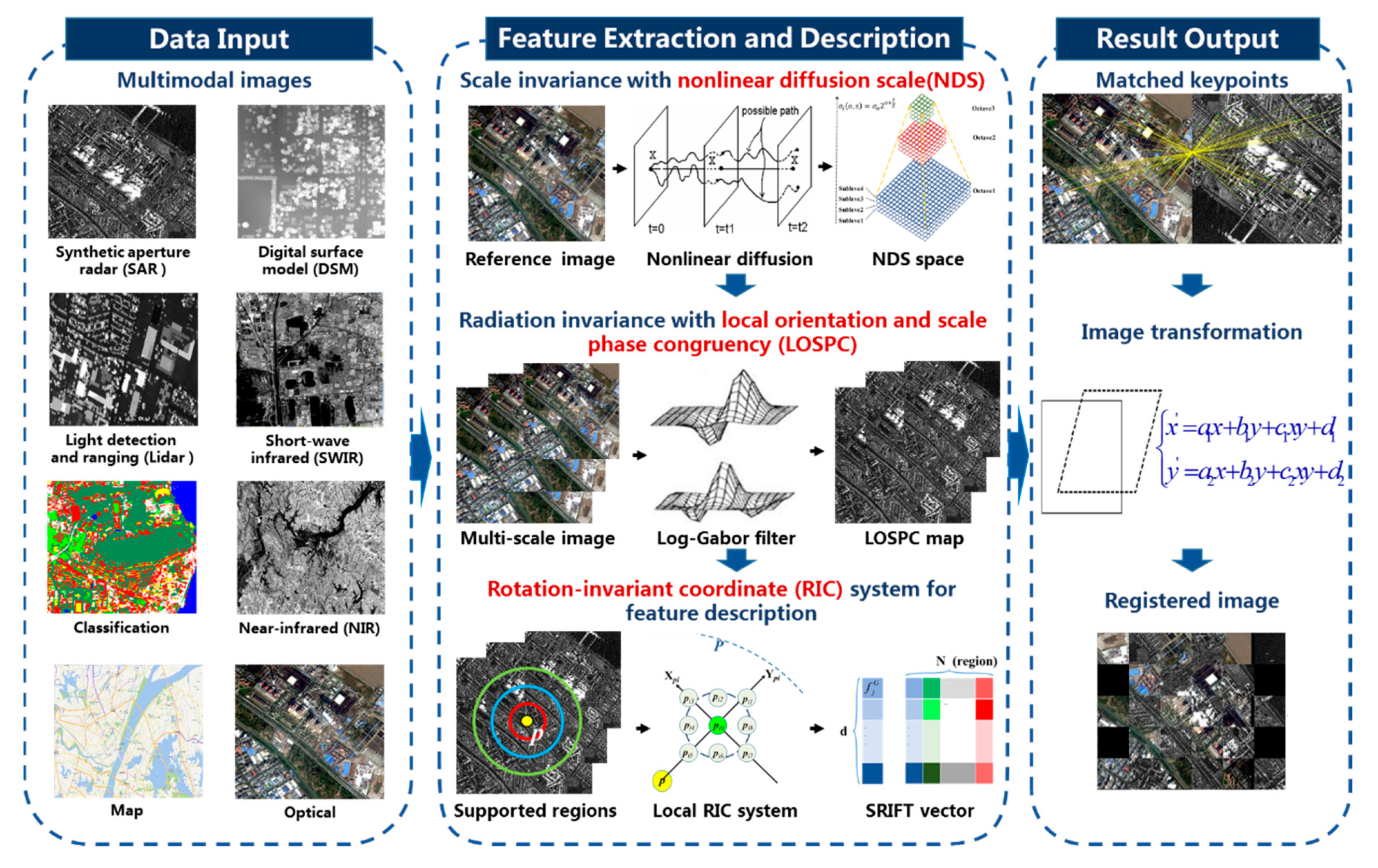
:The nonlinear radiation distortions (NRD) among multimodal remote sensing images bring enormous challenges to image registration. The traditional feature-based registration methods commonly use the image intensity or gradient information to detect and describe the features that are sensitive to NRD. However, the nonlinear mapping of the corresponding features of the multimodal images often results in failure of the feature matching, as well as the image registration. In this paper, a modality-free multimodal remote sensing image registration method (SRIFT) is proposed for the registration of multimodal remote sensing images, which is invariant to scale, radiation, and rotation. In SRIFT, the nonlinear diffusion scale (NDS) space is first established to construct a multi-scale space. A local orientation and scale phase congruency (LOSPC) algorithm are then used so that the features of the images with NRD are mapped to establish a one-to-one correspondence, to obtain sufficiently stable key points. In the feature description stage, a rotation-invariant coordinate (RIC) system is adopted to build a descriptor, without requiring estimation of the main direction. The experiments undertaken in this study included one set of simulated data experiments and nine groups of experiments with different types of real multimodal remote sensing images with rotation and scale differences (including synthetic aperture radar (SAR)/optical, digital surface model (DSM)/optical, light detection and ranging (LiDAR) intensity/optical, near-infrared (NIR)/optical, short-wave infrared (SWIR)/optical, classification/optical, and map/optical image pairs), to test the proposed algorithm from both quantitative and qualitative aspects. The experimental results showed that the proposed method has strong robustness to NRD, being invariant to scale, radiation, and rotation, and the achieved registration precision was better than that of the state-of-the-art methods.
1. Introduction
Image registration is an essential and fundamental task for remote sensing interpretation. It is aimed at registering images obtained from different sensors, different perspectives, different times or different imaging conditions [1], and is an essential preliminary task for image fusion [2], 3D modeling [3], and change detection [4]. With the rapid advance of remote sensing systems, more and more data sources can now be acquired. As a result, the complementary information between multimodal remote sensing images can significantly improve the capacity and effectiveness of the interpretation. However, the efficiency and accuracy of the image registration result greatly affects the performance of the subsequent processing [1]. Nevertheless, for multimodal remote sensing images, a large number of nonlinear radiation distortions (NRD) will be present, as a result of the different physical imaging mechanisms, which brings significant challenges to the image registration.
Generally speaking, image registration methods can be divided into two categories according to the factors (areas and features) on which they are based. The area-based methods adopt the intensity value of the image itself, while the transformation model for the registration is calculated by optimizing a similarity measure between the image to be registered and the reference image. Correlation [5,6,7], mutual information [8,9,10,11,12,13], or frequency-domain information [14,15] can be used as metrics to measure whether the images are registered. However, these area-based methods often reach a locally optimal solution for the optimization of the model transformation, especially when there is NRD among the images. At the same time, the optimization process for the image conversion parameters is of high computational complexity. The feature-based methods have high robustness to geometric distortion and NRD, so that they are commonly adopted in the registration of multimodal remote sensing images. The feature-based methods achieve the matching goal by identifying the reliable characteristic correspondence between the images, and they are not directly based on the image intensity [16]. The features considered by the feature-based methods include point features [17,18,19], line characteristics [20], and structural features [21,22]. Scale-invariant feature transform (SIFT) [23] is a classic feature point matching method. A number of improved versions of SIFT have since been developed, including affine SIFT (ASIFT) [24], speeded-up robust features (SURF) [25], the SIFT-like algorithm for synthetic aperture radar (SAR) imaging (SAR-SIFT), and principal component analysis SIFT (PCA-SIFT). When SIFT or one of its improved algorithms is used to describe the features, the estimated reference direction must be specified, to make the descriptions more unique and robust to the rotation. Image registration based on features is confronted with two problems: (1) in the feature description stage, the estimation of the principal orientation is often prone to error when it is based on the local features of the image, and a lot of corresponding points will be removed due to incorrect principal orientation estimation; and (2) in the feature matching stage, due to the significant NRD, a feature detection result for an image can often not be found, so that there are many abnormalities in the matching result.
In recent years, research into deep learning has exploded in the computer vision field [26,27]. In the study of medical image registration, deep learning has been used to model the relationship between different modal images [28,29]. However, studies of remote sensing image registration based on deep learning are relatively rare, especially for multimodal remote sensing images [30,31,32,33]. The main reasons for this are as follows: (1) Compared with natural or medical images, remote sensing images have an extensive range, complex distortion, and weak uniqueness of targets. It is also common in remote sensing images that the same ground object type presents different forms, or the same form corresponds to different ground object types. (2) Compared with the large number of natural image datasets that can be used for training, manually annotated remote sensing image datasets are very rare. The labeling of remote sensing images needs considerable expert knowledge and manpower. Furthermore, the application of a model trained on natural images to remote sensing registration tasks is impractical. (3) Deep learning is essentially a method of supervised learning, but it is almost impossible to use a model trained on one modal image to register another modal image. For example, the performance of the LiDAR and optical image registration task can be unsatisfactory when using the SAR and optical image training model. Therefore, there is a need to develop a universal handcrafted descriptor for the multimodal remote sensing image registration task, from the perspective of the physical radiation mechanism and the imaging geometric model, in the case of limited training data.
In this paper, we propose a scale-radiation-rotation-invariant feature transform (SRIFT) algorithm for the registration of multimodal remote sensing images. The contributions of this paper can be summarized as follows:
(1) A modality-free multimodal remote sensing image registration method is proposed, which can handle the scale, radiation, and rotation distortions at the same time. The structural characteristics are captured, in which the same kind of ground object will present a similar structural distribution. Thus, the corresponding features of the images are mapped into a unified space to establish a one-to-one relationship.
(2) The nonlinear diffusion scale (NDS) space is constructed using a nonlinear diffusion filter, instead of a Gaussian filter, to preserve more structure and detail information, which is of great importance for feature extraction for the registration. The structural characteristics are captured by computing the local orientation and scale phase congruency (LOSPC) value in the NDS space of the image. The minimum and maximum moment maps of LOSPC are then used to detect the remaining points. Rotation invariance depends on a rotation-invariant coordinate (RIC) system in the feature description stage. The points in the neighborhood are statistically calculated through a continually changing local coordinate system, which itself realizes rotation invariance, without the need for the estimated orientation to be assigned.
The rest of this paper is organized as follows. The related work is introduced in Section 2. Section 3 details the process of image registration using the SRIFT algorithm. In Section 4, the experimental results obtained using both simulated and real multimodal remote sensing images are provided for the experimental verification and analysis. A summary and our conclusion are presented in Section 5.
2. Related Work
For the registration of homologous images, the pixel basis of the above methods is the intensity or the gradient of the image; however, for multimodal images, the structural information presented in the image by the same point on the ground will be entirely different, due to the NRD caused by the different imaging mechanisms. As a result, the above methods will match many pseudo-corresponding features.
With regard to multimodal remote sensing image registration, scholars have put forward various descriptors on the basis of structural information [34,35]. Compared with gradient information, structural information is less sensitive to nonlinear intensity changes [36]. For example, the edge-oriented histogram (EOH) descriptor designates the shape and contour information of the local image centered on each keypoint, instead of the gradient [37]. The partial intensity invariant feature descriptor (PIIFD) was proposed to solve the problem of the relative gradient direction of the corresponding points [38]. A descriptor for the distribution of internal geometric structures was introduced for images captured on a log-polar grid, which is known as the local self-similarity (LSS) descriptor [39]. A dense LSS (DLSS) method was used to process the registration of optical and SAR images in [40]. The histogram of oriented phase congruency (HOPC) [41] algorithm was extended on the basis of the phase congruency algorithm, and its description process adds phase direction statistics to increase the robustness. Radiation-invariant feature transform (RIFT) [42] also considers the phase congruency, and presents a maximum index map, instead of the gradient, in the feature description. The phase congruency-based structural descriptor (PCSD) [43] has also been successful in optical and SAR image registration without rotational distortion.
In this section, the HOPC and RIFT algorithms are introduced as typical registration methods for multimodal remote sensing images.
The HOPC method successfully introduces an oriented phase congruency algorithm into the automatic registration of remote sensing images, while innovatively mapping the two images acquired under different physical mechanisms into a unified space. Therefore, the corresponding features that cannot be mapped one by one can be mapped in this space. However, there are three significant deficiencies in HOPC: (1) it needs relatively accurate geographic information (or rough geometric correction) for the images in the execution process. However, many multimodal remote sensing images do not contain accurate geographic information. (2) As a template matching algorithm, it is sensitive to geometric distortion, such as rotation and scale. (3) It uses the Harris corner detector, which is very sensitive to NRD when extracting feature keypoints.
The RIFT algorithm was developed on the basis of the limitations of the HOPC algorithm. It also uses a phase congruency algorithm for reference in the stage of mapping the corresponding features, but it adopts a novel descriptor for the feature description. The RIFT algorithm is a method of describing the features per-pixel, which also takes rotation invariance into account. However, its rotation invariance and robustness are not outstanding, because of the possibility of losing the spatial information, and the time-consuming nature of its calculation process. Furthermore, it is not scale-invariant. The main disadvantages of the RIFT algorithm are as follows: (1) the RIFT algorithm adopts a “convolution sequence ring” to deal with the rotation distortion of the images, which may lose some spatial information, resulting in insufficient unique feature vectors being generated and unfavorable feature matching; and (2) the RIFT algorithm does not consider the scale invariance, so it is susceptible to scale changes.
Although image registration has been the subject of numerous studies over the last few decades, there is still no unified registration framework that can automatically register multiple multimodal images while considering the scale and rotation distortions.
3. Image Registration Based on SRIFT
In this section, we describe the proposed SRIFT method in detail. Figure 1 presents a registration flowchart based on SRIFT. The highlighted feature extraction and matching parts in the second column of the figure represent the main innovations of this paper. The first two steps of the algorithm involve solving the problem of feature extraction, and the last step involves the feature description. Initially, the NDS space is constructed using a nonlinear diffusion filter, instead of a Gaussian filter, to preserve more structural and detail information, in order to achieve scale invariance. The structural characteristics are then captured by computing the LOSPC values, in which the same kind of ground object will present similar structural distributions. Finally, the RIC system is applied, which itself realizes rotation invariance, without the need for the estimated reference orientation.
The fundamental reason that restricts the accurate registration of multiple source images is the nonlinear mapping of the corresponding features caused by the existence of NRD. Therefore, as long as the corresponding features can correspond one-to-one, the registration problem for the different source images can be transformed into a registration problem for the same source images. Hence, in the third column of Figure 1, we can use a large number of methods that have been well studied by predecessors in the field of homologous image registration for the image transformation and resampling.
3.1. Scale Invariance Through the Nonlinear Diffusion Scale (NDS) Space
In the construction process of the scale space, the SIFT algorithm uses a Gaussian space, which is generated by convolving the original image with a Gaussian filter of different scales. However, some structure and contour information in the image will be lost in the filtering process because the Gaussian filtering is a kind of smoothing operator, and the loss of information will adversely affect the feature extraction of multimodal remote sensing images with NRD.
The detailed structural information needs to be included as much as possible when the scale space is established. Inspired by anisotropic diffusion [44], a nonlinear diffusion function, instead of a Gaussian function, is adopted to generate the scale space of the image in the proposed algorithm:
where is a scale parameter, is a bifurcation operator, is the gradient operator, is the Laplace operator, and is the diffusion coefficient. In the particular case where the nonlinear diffusion is assumed to be isotropic, is a constant, and the above formula is the same as a Gaussian function. Since there is no analytical solution to the nonlinear diffusion equation, a numerical method is needed to approximate the solution. Equation (1) generates the following relationship after being applied as an additive operator splitting strategy:
where is an identity matrix, signifies the time step, and represents the direction. Along the l-th coordinate axis, matrix is established accordingly.
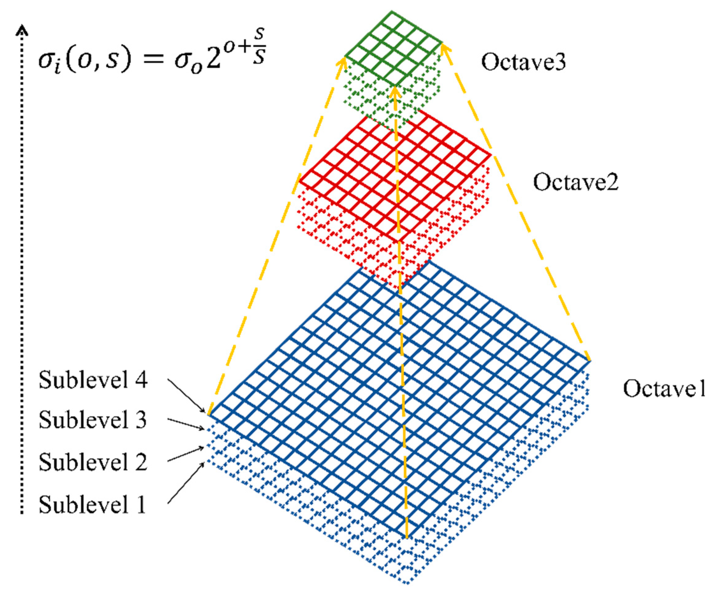
The same tactic is applied as is used in SIFT, where the scale space is discretized into a series of octaves and sublevels. By using the original image as an initial condition, the multi-scale space for the multimodal image is generated as a series of smoothed images. The scale values are equal to:
where values are calculated from the following expression:
where is the base scale level; and are the indices of octave and sublevel , respectively; and is the total number of smoothed images. It is notable that the image is downsampled when the last sublevel is reached in each octave, and the downsampled image is used as an initial image for the next octave, as shown in Figure 2.
Through the construction of the NDS space, the attained multi-scale images can preserve the structural and detail information. Therefore, it is anticipated that the proposed SRIFT method will be able to detect many more keypoints.
3.2. Radiation Invariance Through Local Orientation and Scale Phase Congruency (LOSPC)
It should be noted that the orientation and scale referred to in this section are different from the orientation referred to in Section 3.1 and the scale referred to in Section 3.3. The orientation and scale referred to in this section are aimed at giving the spatial mapping more structural information, and the orientation referred to in Section 3.1 and the scale referred to in Section 3.3 are taken into consideration to make the feature description more stable.
3.2.1. Frequency Domain Spatial Mapping via Phase Congruency
The feature extraction can be carried out after the establishment of the multi-scale space. To solve the NRD problem, the LOSPC algorithm is proposed to construct a unified and describable space, which is a prerequisite for the subsequent extraction of the corresponding features.
Feature extraction in the spatial domain of multimodal images often fails due to the distortion of the grayscale and gradient information. Instead, in the frequency domain, an image is decomposed into amplitude and phase components, where the same kind of ground object will present similar structural distribution features in the multimodal images. Phase congruency can be used to measure the degree of local phase information consistency at various angles [45]. Instead of considering the locations with the maximum intensity gradient as being the edges, the phase congruency model regards the edge points as being where the Fourier components are maximally in phase [46]. The phase information is the measurement describing the structural distribution features of the image in the frequency domain.
A 2-D phase congruency operator is developed for the calculation of the phase congruency of any point in the plane, which is a theory that can also be applied to image processing [47]. We define an image as , and then the odd-symmetric part and even-symmetric part can be obtained by convolving the image with the log-Gabor wavelet transform:
where, in scale and orientation , and stand for the even-symmetric and the odd-symmetric log-Gabor wavelets, respectively. The amplitude and the phase parts of image can be expressed as:
When all the scales and orientations are considered, the results of the two-dimensional phase congruency are calculated as follows:
where is a weight function; is a constant with a minimal number; the action is to prevent negative values, which means that when the value is negative, its result is 0; and is a phase deviation function, which is defined as:
where
Through the above formulas, each pixel in the image can acquire a statistical value for the phase congruency, which contains orientation and scale information and is based on the structural distribution. In different multimodal remote sensing images, the same ground object will have the same structural distribution. Although it has undergone different physical radiation mechanisms, the value of the phase congruency will be the same.
3.2.2. Feature Point Extraction
In the feature extraction stage, it is necessary to design a feature extraction method based on the statistical index of the phase congruency. Equation (8) is used to calculate the phase congruency of the image pixel by pixel, so an edge graph can be obtained, which is robust to the various multimodal remote sensing images. However, when the image is calculated with log-Gabor filters in different directions, the phase congruency should change with the direction of the filter. Unfortunately, this information is not recorded. Therefore, in order to prevent the phase congruency information changing with the direction, it is necessary to calculate the moment of the phase congruency in each direction, and to record the values with the change of direction. In moment statistics, the principal axis indicates that the moment at this axis is the smallest [46]. The moment perpendicular to the principal axis is the maximum moment. If the maximum moment is large, it is likely to be an edge point in the image, while if the minimum moment is large, it is likely to be a corner point in the image.
According to the moment analysis algorithm, the following three statistics can be obtained from the typical moment calculation formula:
The angle of the principal axis can then be calculated by the following formula:
After obtaining the principal axis, the minimum moment and maximum moment can are calculated as follows:
By detecting the extreme values of the maximum moment and the minimum moment on the image, a group of feature points can be obtained, which are called keypoints. The feature extraction step has now been completed. The detection of feature points is undertaken in the frequency domain, instead of the traditional approach of the feature points being detected directly from the image intensity or gradient value, so that the proposed method can better deal with the NRD in multimodal remote sensing images. These keypoints are then used in the subsequent feature matching.
3.3. Rotation Invariance Through a Rotation-Invariant Coordinate (RIC) System
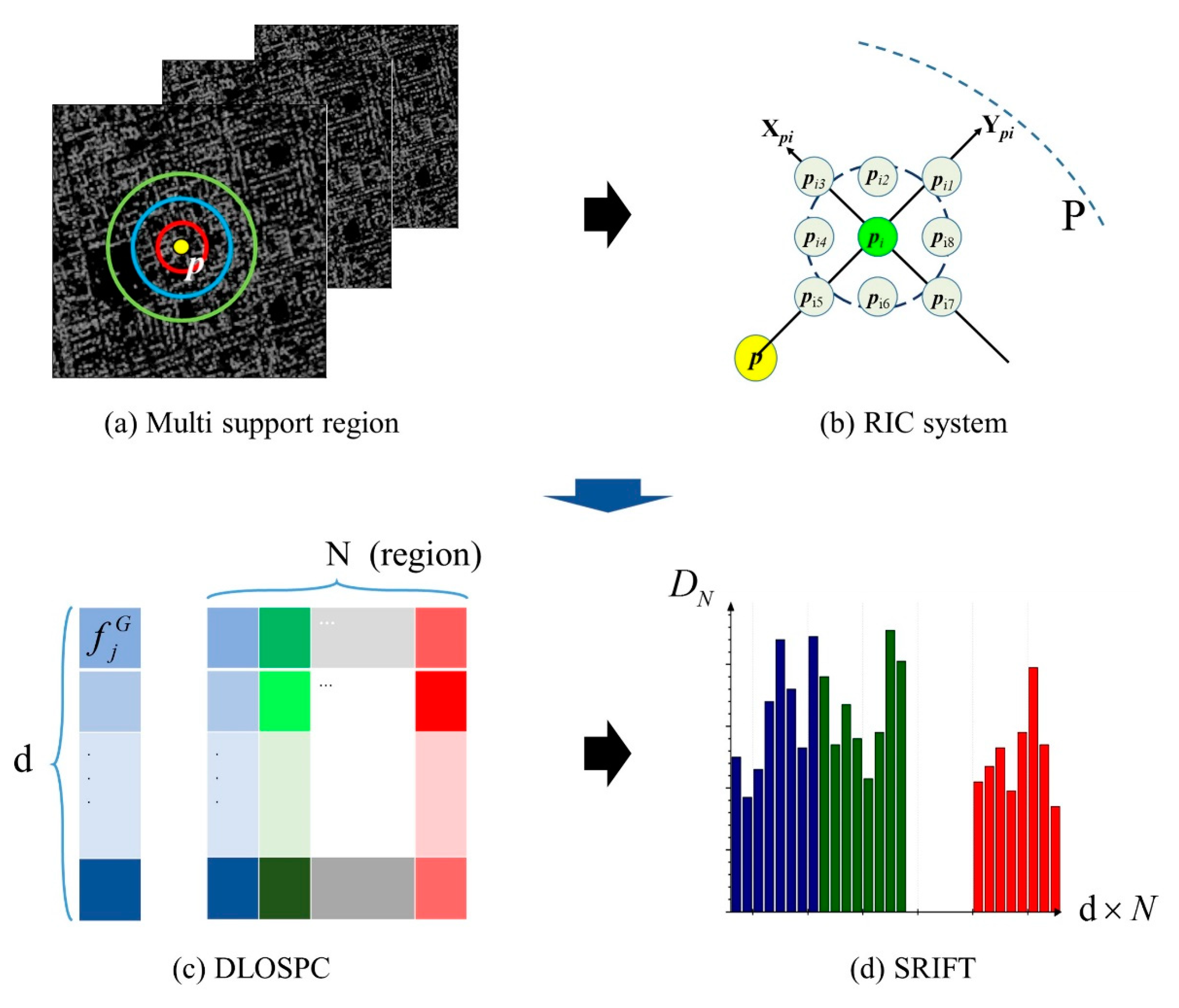
After extracting a large number of stable feature keypoints, these points then need to be described. The process of description should consider the change of features with the transformation of the various influencing factors, and should highlight the uniqueness of the features, to ensure the uniqueness of the subsequent feature matching. In order to achieve rotation invariance in the feature description stage, inspired by the work of “aggregating gradient distributions into intensity orders” [48], a RIC system is proposed. In the feature description, the sample points neighboring a keypoint are statistically calculated through a constantly changing local coordinate system, which itself realizes rotation invariance, without the need for the dominant direction. Firstly, we select several candidate support regions, according to a certain proportion. The difference between local orientation and scale phase congruency (DLOSPC) histogram is then calculated in the local RIC system at each sub-region. Finally, by connecting each DLOSPC vector in the image neighborhood of the multiple support regions, the descriptor is constructed. A flowchart of the construction of the descriptor is shown in Figure 3.
3.3.1. The Local Rotation-Invariant Coordinate (RIC) System
In order to realize the rotation invariance of the proposed algorithm, the descriptor of each support region is calculated by the local RIC system. Specifically, a RIC system is built around each keypoint. is a point in one support region of the keypoint , where the line connecting and is set as the y-axis, and the direction of the vector is the y-axis direction. We then construct a local Cartesian (x-y) coordinate system. For the sample points , the pixels in the field participate in the calculation in a rotation-invariant manner; that is to say, the local structure in the field of the sample points is retained. Therefore, the feature description in the locally invariant coordinate system is rotation-invariant. A local RIC system for keypoint is then constructed. is set as the origin, i.e., the first pixel along the direction of the y-axis is set to , and then the pixels in the eight fields of are marked as , ,... , as shown in Figure 3b.
3.3.2. The Difference between Local Orientation and Scale Phase Congruency (DLOSPC) in the RIC System
For each sample point , its difference of local orientation scale phase congruency can be computed in the local RIC system. The calculation formula is as follows:
where are point ’s neighboring points along the x-axis and y-axis in the local x-y coordinate system, and stands for the intensity at on the LOSPC map. The difference and orientation can then be computed as:
Note that is converted into the range of , along with the values of and . The gradient of is then constructed as a d-dimensional vector represented as . To do this, is divided into equivalent boxes as , and then is assigned to the different boxes by linear distance weighting :
where is the angle between and .
3.3.3. Construction of the Keypoint Descriptors Through Multiple Supported Regions
As shown in Figure 3, it is not sufficient to distinguish correct matches from a large number of wrong matches with a single support region. Furthermore, two non-corresponding keypoints may exhibit similarity in some support regions. However, the two corresponding keypoints should have a similar appearance in all the support regions of different sizes, although there may be some small differences due to positioning errors of the keypoints and area detection. That is, when multiple support regions are used, mismatches can be better handled than when only a single support region is used.
N nested support regions are selected with the different radius , centered on a keypoint, as shown in Figure 3a. The minimum support region is defined as , and then the other support regions can be expressed as , where represents the size of the -th support region. is defined as in this paper, so that the radius increments of the support regions are equal.
The cumulative vectors are combined to form a vector in each support region, and then the cumulative vectors of the different support regions are connected together to describe the features of the keypoint. is used to represent the cumulative vector for a support region:
Finally, all the vectors calculated in the N support regions are connected together to form the final descriptor .
4. Experiments and Analyses
The performance of the proposed SRIFT method was tested in both simulated and real-data experiments. In the simulated experiments, the robustness of the algorithm to geometric distortion was tested by artificially adding various scale and rotation distortions. In the real-data experiments, the registration performance obtained by the SRIFT method was compared to that of eight state-of-the-art image registration methods (SIFT [23], ASIFT [24], SAR-SIFT [49], PSO-SIFT [50], DLSS [40], HOPC [41], PCSD [43], and RIFT [51]), with different modal image pairs.
4.1. Experimental Description
The aim of the simulated experiments was to analyze the ability of SRIFT to resist different image geometric distortions, including scale, rotation, and combined distortions.
4.1.1. Simulated Dataset Construction and Evaluation
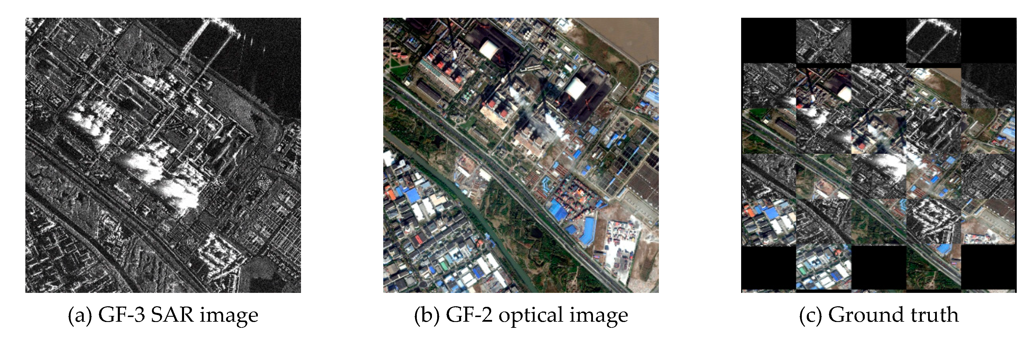
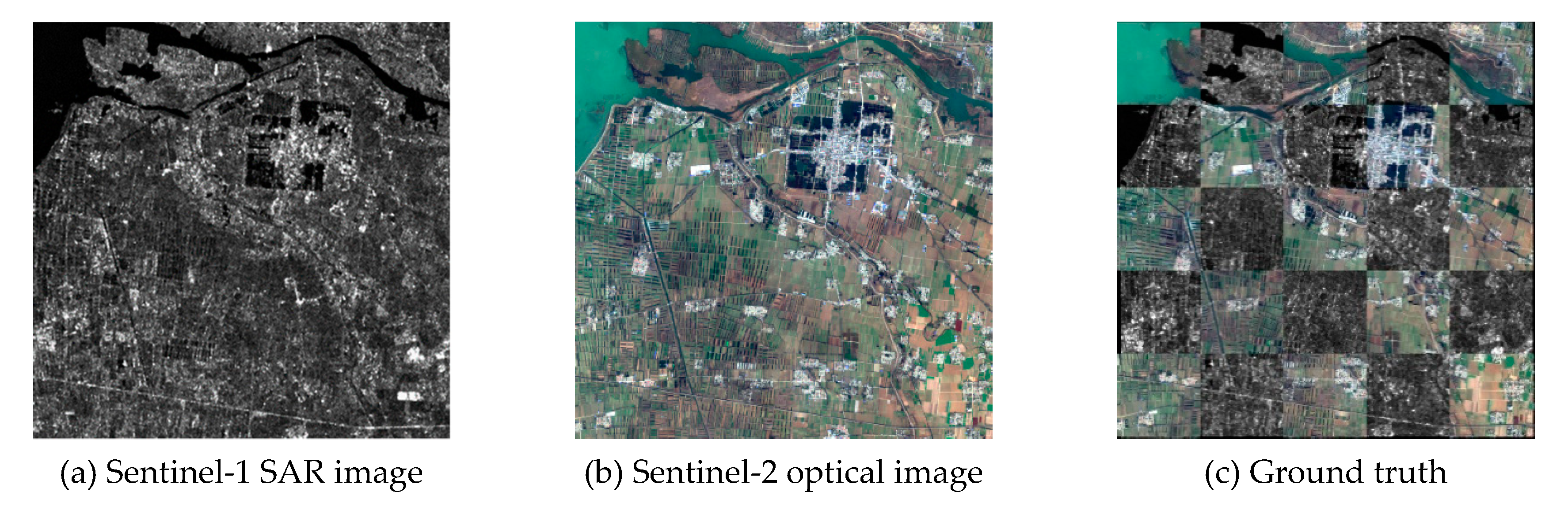
The simulated dataset experiments involved two sets of images, in which the ground truth had been geometrically corrected and manually checked, so that the positioning accuracy was better than one pixel, as shown in Figure 4 and Figure 5. Figure 4a,b show the first case of a SAR and optical image pair from Shanghai, China, which were acquired by the GF-3 and GF-2 remote sensing satellites, respectively. Figure 5a,b show the second case of a SAR and optical image pair from Leshan, Sichuan province, China, which were acquired by the Sentinel-1 and Sentinel-2 remote sensing satellites, respectively.
The experimental parameters were set as follows. The simulated datasets were generated by scale and rotation transforms with regard to the ground-truth images, where the images were resampled by 0.5, 0.3, and 0.25 times for the scale transforms and rotated by 10, 30, and 90 degrees, respectively. Therefore, the geometric distortion parameters of the images were known and could be used to calculate the accuracy of the registration results.
If the sensed image can be regarded as an initial condition, and transform matrices of the simulated dataset can be denoted as , then image can be transformed into an image . When the image has keypoints , the corresponding keypoints in the image are , and are regarded as the ground truth.
The transform matrices calculated after registration are appropriately denoted as , and the root-mean-square error (RMSE) is used to evaluate the registration accuracy of the simulated data images. The higher the RMSE, the worse the accuracy. The RMSE is defined as:
where is the residual error, which is calculated between the transformation parameters and the transformation parameters . is solved by the corresponding points after registration, while is given by the ground truth. The RMSE is measured in pixels. The keypoints in which the residual error is less than two pixels are regarded as correctly matched. The number of correctly matched () corresponding keypoints is an important evaluation metric for image matching.
4.1.2. The Overall Performance Comparison
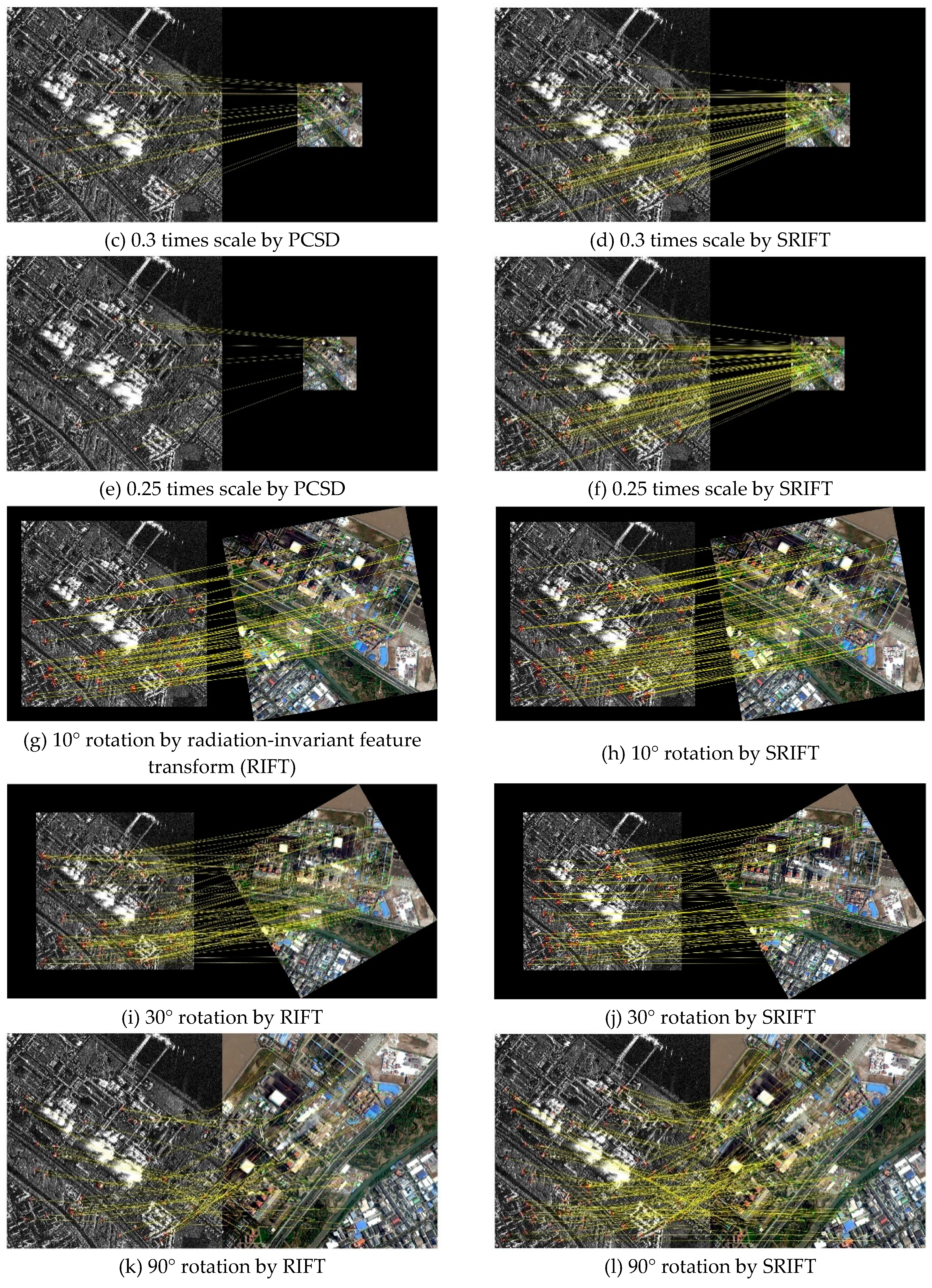
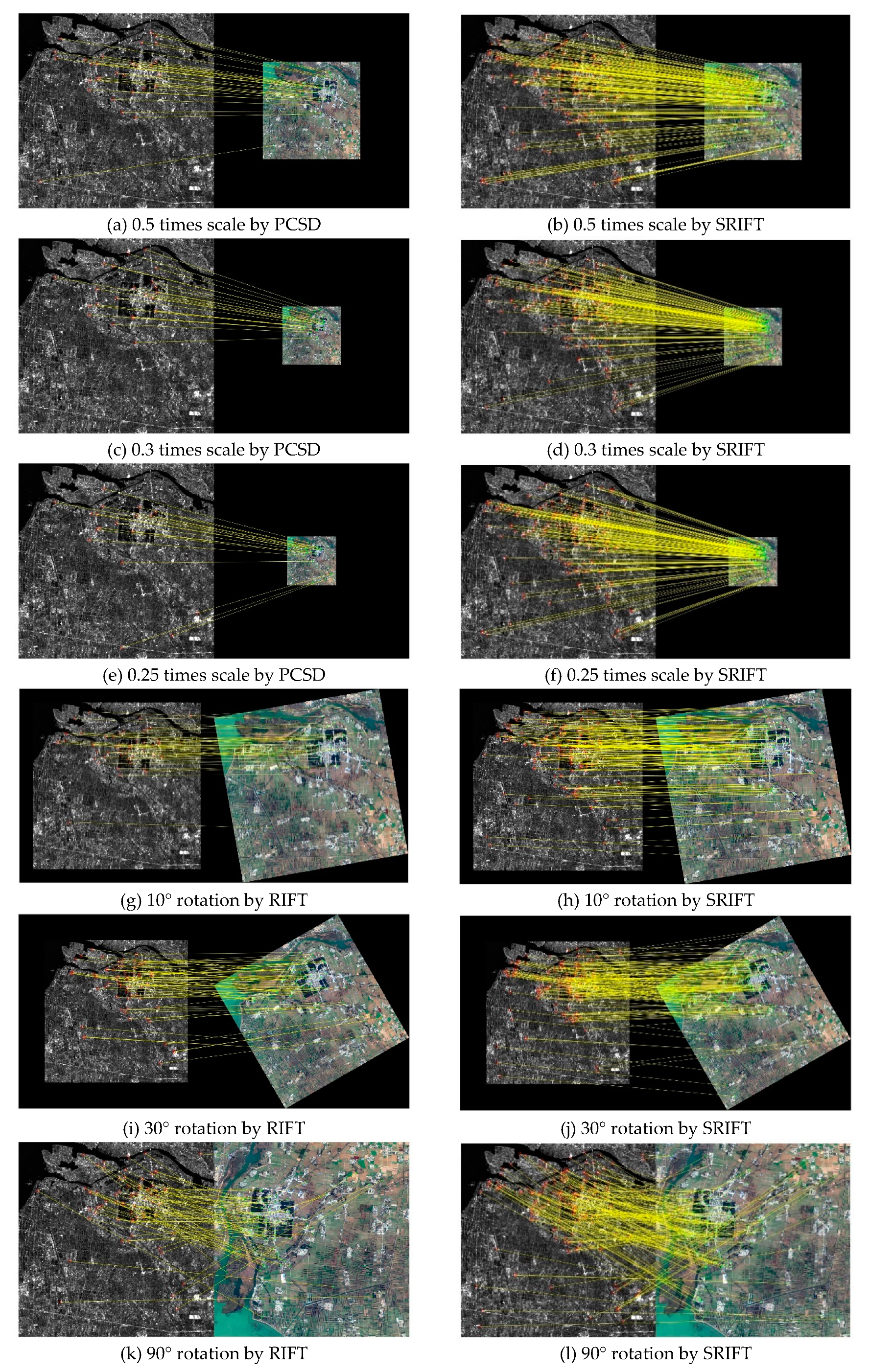
Qualitative evaluation: the overall performances for the corresponding points obtained by the proposed SRIFT method on the simulated datasets are shown in Figure 6 and Figure 7, in which the best results of the state-of-the-art comparison methods for each distortion case are selected for display. As can be seen, the corresponding points obtained by SRIFT are abundant, evenly distributed, and accurately located, and can thus be used to calculate the image transformation model, and then register the image with the calculated model to obtain the registration result.
From the experimental results, it can be seen that, in the process of keypoint extraction, the SRIFT algorithm can extract points characterized by a uniform distribution and sufficient quantity, but after the feature matching and error elimination, the regions with rich shape and texture, and high structural uniqueness, retain more keypoints. In contrast, flat regions with less texture or regions with less structural uniqueness and more repeated textures have fewer corresponding keypoints. Compared with the registration methods based on intensity or gradient, the SRIFT algorithm is essentially a kind of structural descriptor. The description vector of each keypoint is the geometric statistics in an image patch of a specific size centered on this keypoint. In other words, a SRIFT vector describes all the structural information of an image block centered on the keypoint, with a specific sized region (the region sizes are described in Section 3.3.3) as the radius. When the structural information of two image blocks is highly similar, their center points are the registered keypoints.
Quantitative evaluation: Table 1 and Table 2 list the RMSEs of the simulated data image registration results of the SRIFT method, as well as those of the other state-of-the-art image registration methods.
As can be seen from Table 1 and Table 2, the registration accuracy of the SRIFT algorithm is consistently the highest. Compared with SIFT and ASIFT, the SRIFT algorithm has a better feature extraction and description ability for multimodal images. SAR-SIFT, PSO-SIFT, DLSS, HOPC, PCSD, and RIFT are specially designed for multimodal image registration. Compared with the template matching algorithms such as DLSS and HOPC, SRIFT can resist the various scale and rotation distortions. Compared with feature matching algorithms such as SAR-SIFT, PSO-SIFT, PCSD, and RIFT, SRIFT can overcome more complex image geometric distortions. For a more detailed analysis of the results of the state-of-the-art algorithms, see Section 4.2.3.
4.1.3. The Ability of the Algorithm to Resist the Scale and Rotation Distortion
To test the robustness of SRIFT to image scale and rotation distortion, simulated images were generated by resizing the image using a scale change factor from 1 to 10 with different intervals and rotating the image using a rotation change factor from 0 to 360 with an interval of 30. The matching performance of the proposed method with scale and rotation distortion is shown in Figure 8.
As shown in Figure 8a, when the image scale difference is between one time and four times, the precision of the proposed method does not decrease significantly when the scale factor increases. The proposed method maintains a good performance when the scale factor is less than four times. We can, therefore, conclude that the proposed method is robust for scale difference. However, when the scale difference increases to more than five times, the correct matching point number plummets. From Figure 8b, for rotation distortion at any angle, the proposed SRIFT algorithm extracts relatively abundant corresponding points.
4.2. Experiments with Real Images
In the real-data experiments, the registration results obtained by the proposed method were compared to those obtained by eight state-of-the-art methods: SIFT, ASIFT, SAR-SIFT, PSO-SIFT, DLSS, HOPC, PCSD, and RIFT.
4.2.1. Real Datasets
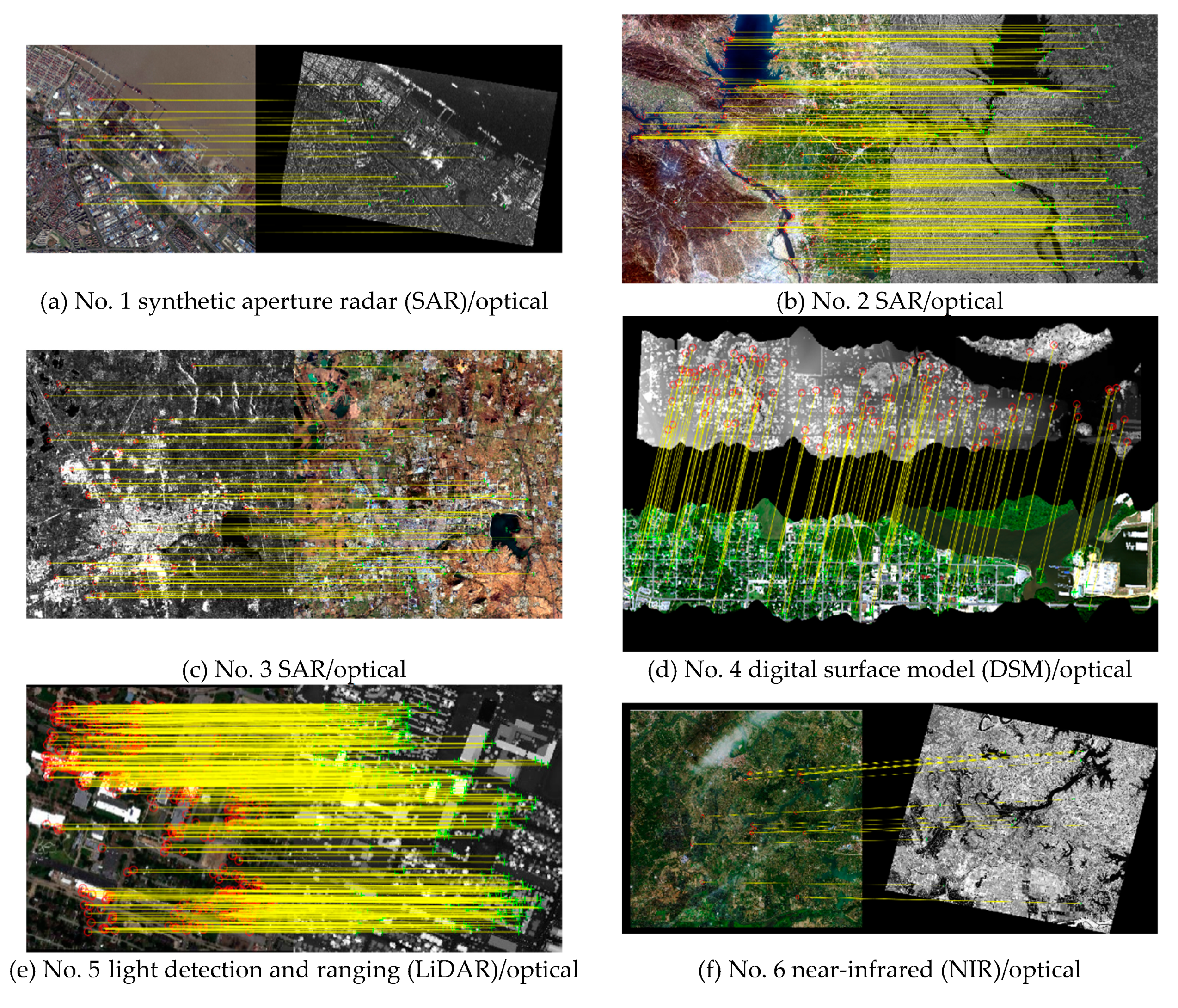
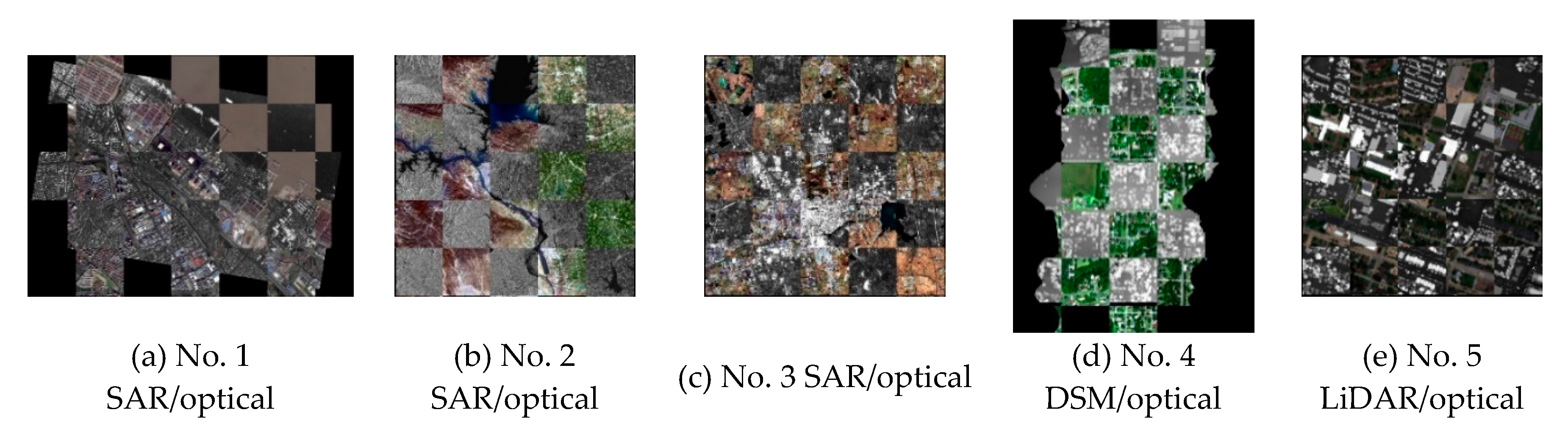
In the real-data experiments, nine sets of multimodal images were selected: SAR/optical, DSM/optical, LiDAR/optical, NIR/optical, SWIR/optical, classification/optical, and map/optical images, which are shown in Figure 9 and described in Table 3.
Figure 9a shows the first SAR/optical image pair covering an urban area. These images were acquired by the GF-3 and GF-2 remote sensing satellites, respectively. The resolution of the SAR image was set to 1 m, referring to the 4-m resolution of the optical image through panchromatic and multispectral fusion. The image sizes are 4865 × 3504 and 3979 × 3619 pixels, respectively.
Figure 9b shows the second SAR/optical image pair covering a mountainous and water area. These images were acquired by the GF-3 and GF-1 remote sensing satellites, respectively. The resolution of the SAR image was set to 8 m, referring to the original 8-m resolution of the multispectral optical image. The image sizes are both 6000 × 6000 pixels.
Figure 9c shows the third SAR/optical image pair, again covering a mountainous and water area. These images were acquired by the Sentinel-1 and Sentinel-2 remote sensing satellites, respectively, in November 2017. The resolution of the SAR image was set to 10 m, referring to the original 10-m resolution of the multispectral optical image. The image sizes are both 2000 × 2000 pixels.
Figure 9d shows the DSM/optical image pair covering an urban area. These images were acquired by manual production and an unmanned aerial vehicle (UAV), respectively, in May 2017. The resolution of the DSM was set to 1 m, referring to the original 1-m resolution of the optical image. The image sizes are both 1200 × 1200 pixels.
Figure 9e shows the LiDAR/optical image pair covering an urban area. These images were acquired by a LiDAR system and aerial photography, respectively, in June 2017. The image resolutions are 2.5 m, and the image sizes are 349 × 349 pixels.
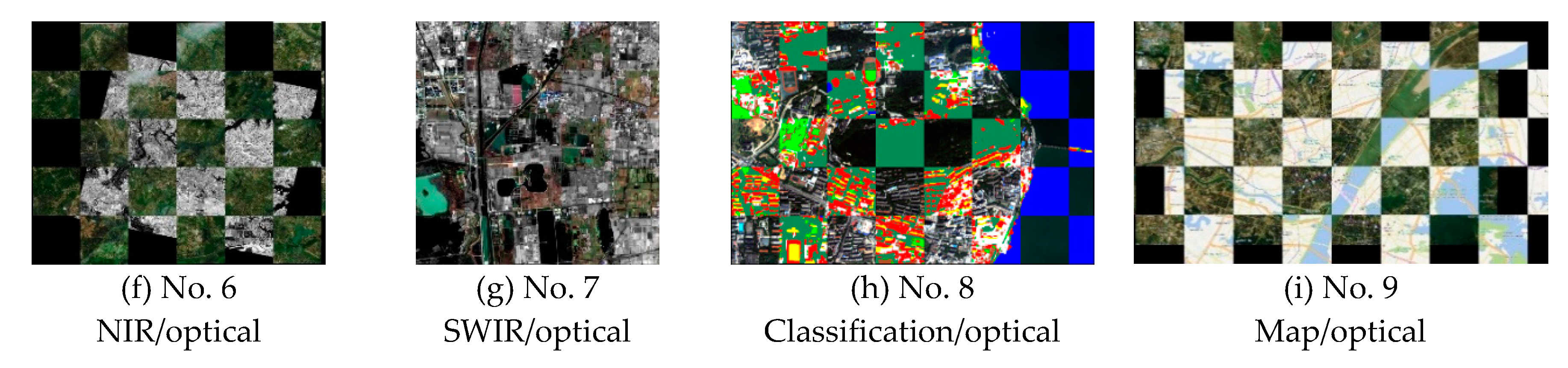
Figure 9f shows the NIR/optical image pair covering a farmland and water area. The NIR image was acquired by the GF-2 remote sensing satellite in April 2016, and the optical image was downloaded from Google Earth. The image resolutions are 3.2 m and 4 m, and the sizes are 1202×1011 and 1014 × 950 pixels, respectively.
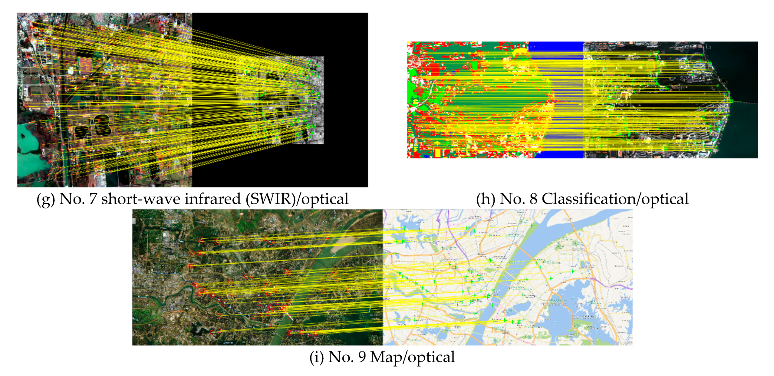
Figure 9g shows the SWIR/optical image pair covering a farmland and water area. These images were both acquired by the Sentinel-2 remote sensing satellite. The image resolutions are 20 m and 1 m, respectively, and the image sizes are 1000 × 1000 pixels.
Figure 9h shows the classification/optical image pair covering an urban area. These images were respectively acquired by manual production and the GF-1 remote sensing satellite in March 2013. The resolution of the classification image was set to 4 m, referring to the original 4-m resolution of the multispectral optical image. The image sizes are both 640 × 400 pixels.
Figure 9i shows the map/optical image pair covering an urban area. These images were downloaded from Google Earth. The image resolutions are 4 m, and the image sizes are 1867 × 1018 pixels.
There is severe distortion between all these images, especially radiation distortion. They therefore pose a significant challenge for the image registration algorithms.
4.2.2. Ground-Truth Setting and Evaluation Metrics
Ground truth is essential for the quantitative evaluation of registration. However, due to the different sensors and/or different perspectives in multimodal images, it is often impossible to achieve a one-to-one correspondence between pixels. Therefore, precise geometric correction is required for every set of image pairs in real datasets, and then the geometric correction transformation parameters are approximated as the ground truth. In detail, a certain number of precise corresponding points are artificially selected in each pair of images, and the image transformation parameters are then solved using these points. The images are registered using these parameters, and the registration result is manually checked. If the result is not accurate, the artificial selection is repeated until the two image pairs are accurately registered. When evaluating the registration accuracy, the image transformation parameters estimated by the registration algorithm are used to calculate the residuals of the artificially selected corresponding points.
For the real-data experiments, three evaluation metrics were selected to evaluate the registration performance. The precision is expressed as , where is the total number of corresponding keypoints. The definitions of and RMSE have been given in Section 4.1
4.2.3. Registration Performance Comparison
Qualitative comparison: Figure 9 intuitively shows the corresponding point-line diagrams obtained by the SRIFT algorithm in the real-image experiments, where the number and distribution of the corresponding points reflect the robustness and applicability of the algorithm. Figure 10 uses checkerboard mosaicked images of the nine groups for the qualitative evaluation, where the continuousness of the sub-region edges of the images directly reflect the accuracy of the registration.
Through the analysis of the above experimental results, the following conclusions can be drawn. The proposed SRIFT registration algorithm was able to obtain satisfactory results on all nine datasets of various multimodal remote sensing images. When dealing with the multimodal image registration task, the SRIFT algorithm fully considers the influence of NRD in the feature extraction, as well as the feature description, so that it can extract a large number of stable and evenly distributed feature points. The SRIFT algorithm can also resist image scale and rotation distortion, and the registration image has a high coincidence degree with the reference image.
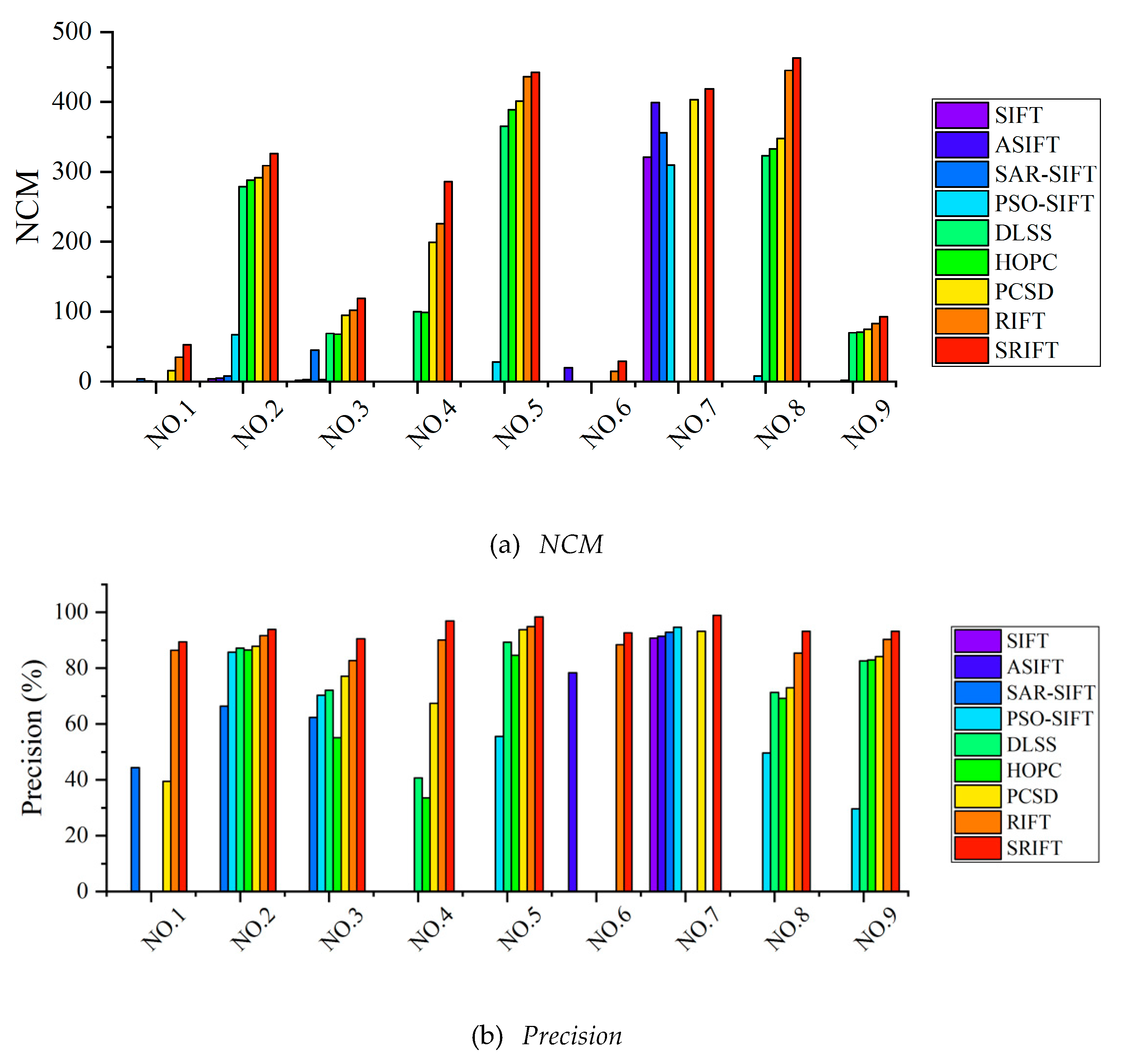
Quantitative comparison: Figure 11 quantitatively reflects the registration effect and accuracy of the eight algorithms on the nine sets of data with the three measurement indices introduced in Section 4.2. Figure 11a is the line chart of , where the higher the value of , the more keypoints are correctly matched, which reflects the ability of the different algorithms in the feature matching stage. Figure 11b is the line chart of the precision, where the higher the value, the higher the proportion of correct matching points in all the matching points, reflecting the ability of the different algorithms in the feature description stage. Figure 11c is the line chart of the RMSE, where the lower the value, the higher the registration accuracy, reflecting the overall registration ability of the different algorithms.
As can be seen in Figure 11, SRIFT achieves the best precision. RIFT ranks second and PCSD ranks third. The basic idea of the HOPC and DLSS algorithms is to divide the images into blocks by counting the local information of each image block, and to then integrate the blocks into the overall information. Their performance generally lies in the middle level among the eight compared methods. The SIFT and ASIFT algorithms are not designed for multimodal data, so that they perform the worst of all. A detailed analysis of each method is presented in the following.
Due to the SIFT algorithm detecting feature points directly based on the intensity, and using gradient information for the feature description, which is sensitive to NRD, SIFT only obtains good registration results for the SWIR/optical case. In the SWIR/optical case, the sensors are on the same satellite, and the two sources have little difference in radiation mechanism, so that the image registration is relatively easy.
The results of the ASIFT algorithm are slightly better than those of SIFT. The registration results cannot be obtained for most of the images, but the registration results are better than those of SIFT in the complex set of geometric transforms in the NIR/optical case, because ASIFT is specially designed for affine transformation. ASIFT simulates the scale and the camera direction and normalizes the rotation and the translation.
The SAR-SIFT method was specially designed for SAR imagery, and it relies on a new gradient computation method adapted to SAR images. Therefore, the image registration results for the first three SAR datasets are satisfactory. However, the redefined gradient probability has difficulty in dealing with complex radiation distortion, and the multi-scale Harris detector has insufficient resistance to NRD.
PSO-SIFT achieves the best registration effect among the SIFT-related algorithms, which is due to the fact that PSO-SIFT applies multiple constraints, e.g., the feature distance, and hence results in a better registration.
The DLSS algorithm is an improved version of the LSS algorithm, which divides the template window into spatial regions called “cells.” Each cell contains n × n pixels, and has an overlapping region of half a cell width with the neighboring cell. This method of division is essentially a template matching method, rather than a feature matching method. As a result, DLSS cannot resist the complex geometric distortion, and the registration performance in datasets 1, 4, 6, 7, and 9 is poor.
HOPC uses the Harris detector to detect the feature points. However, the Harris detector is very sensitive to NRD, and it is not universally suitable for all the different types of multimodal images. Therefore, overall, its registration effect is slightly worse than that of DLSS. Moreover, HOPC is similar to DLSS in the blocking strategy, so that HOPC also has a poor effect in images that cannot be registered by the DLSS algorithm.
The RIFT algorithm does not have scale invariance, so its registration effect in the SWIR/optical case is inferior. In order to achieve rotation invariance, RIFT transforms the initial layer to reconstruct a set of convolution sequences with different initial layers, and then calculates a maximum index map (MIM) from each convolution sequence to obtain a set of MIMs. This statistical method only establishes the relationship between the neighborhood pixels of the keypoints and the keypoints themselves, and it destroys the structural relationship between the neighborhood pixels of the keypoints. Therefore, for images with both scale and rotation transformation, the registration effect is weak.
In the feature description stage, the PCSD algorithm adopts a method similar to SIFT, which requires estimation of the main direction, and error in the primary direction estimation causes the extracted corresponding points to be deleted by mistake. In the feature extraction stage of PCSD, the points with the closest cosine similarity to the keypoints in the reference image are matched. However, this method does not take advantage of a phase congruency algorithm in the feature extraction, and its stable alignment points are insufficient.
The analysis of the experimental results confirms the powerful registration ability of the SRIFT algorithm. If the structural information of the images to be registered is similar, the SRIFT algorithm can register the images without considering the distortion of the image intensity.
4.2.4. Computational Cost
An experiment addressing the computational cost of the proposed method and that of some of the comparison methods (SIFT, SAR-SIFT, PCSD, HOPC, RIFT, SRIFT) was undertaken. The average run times of the different methods on the real datasets are shown in Table 4. The experiment is carried out on a computer with an Intel i7-6200U CPU @ 2.30GHz and 8 GB of RAM. All the methods were implemented in MATLAB.
According to Table 4, the SIFT algorithm has the highest computational efficiency, followed by the SAR-SIFT algorithm, because neither algorithm performs phase congruency calculation. Among the four methods that adopt phase congruency (PCSD, HOPC, RIFT, and SRIFT), RIFT shows the highest computational efficiency because it replaces phase congruency with maximum index graph. PCSD and HOPC are in the middle level, but the calculation time of the proposed method is relatively high. Due to the use of the multi-scale space, phase congruency, and RIC system to deal with the NRD, as well as the complex scale and rotation variation, the proposed method is relatively time-consuming. Algorithm optimization and efficiency improvement will be carried out in the future.
5. Conclusions
In this paper, we have presented a modality-free multimodal remote sensing image registration method named SRIFT, which has the advantage of scale, radiation, and rotation invariance, making it suitable for use with different multimodal remote sensing images. The building of a robust NDS space, the definition of a new concept called LOSPC, and the development of a new RIC system are the three main contributions of the proposed SRIFT method. The NDS space is constructed to resist the scale distortion of image pairs with a large difference in gradient distribution. LOSPC is computed in the NDS space of the images, in which the same kind of ground object will present similar structural distributions, and thus the features of these images are mapped into the same space. The idea of the RIC system is that the points in the neighborhood are statistically calculated through a continually changing local coordinate system, which is more suitable for the feature matching task than a global coordinate system, and realizes rotation invariance, without the need for the estimated orientation to be assigned. In the experimental analysis, two simulated datasets and nine sets of real data were used to qualitatively and quantitatively compare the registration performance of SIFT, ASIFT, SAR-SIFT, PSO-SIFT, DLSS, HOPC, PCSD, RIFT, and the proposed SRIFT method. The registration performance of the SRIFT algorithm on the multimodal images with NRD was superior to that of the other state-of-the-art image registration methods. Our future study will focus on research into a correction model and error elimination for multimodal image registration.
Author Contributions
S.C. established the motivation, designed the method, developed the code, performed the experiments, and wrote the manuscript; M.X. and Y.Z. provided funding; A.M. and Y.Z. reviewed and improved the manuscript. All authors have read and agreed to the published version of the manuscript.
Funding
This research was supported by the National Key Research and Development Program of China under grant nos. 2018YFB0504801 and 2017YFB0504202, and in part by the Fundamental Research Funds for the Central Universities under grand no. 2042020kf0014, and in part by the National Natural Science Foundation of China under grant nos. 41622107 and 41801267.
Acknowledgments
The authors would like to thank Yuanxin Ye for sharing the code of the HOPC method and some of the experimental data, and Wenping Ma for sharing the code of the PSO-SIFT method.
Conflicts of Interest
The authors declare no conflicts of interest.
References
- Zitová, B.; Flusser, J. Image registration methods: A survey. Image Vis. Comput. 2003, 21, 977–1000. [Google Scholar] [CrossRef] [Green Version]
- Wu, Y.; Fan, J.; Li, S.; Wang, F.; Liang, W.; Wu, Y.; Fan, J.; Li, S.; Wang, F.; Liang, W. Fusion of synthetic aperture radar and visible images based on variational multiscale image decomposition. J. Appl. Remote Sens. 2017, 11, 025006. [Google Scholar] [CrossRef]
- Hirschmuller, H. Stereo processing by semiglobal matching and mutual information. IEEE Trans. Pattern Anal. Mach. Intell. 2007, 30, 328–341. [Google Scholar] [CrossRef]
- Jia, L.; Li, M.; Zhang, P.; Wu, Y. Sar image change detection based on correlation kernel and multistage extreme learning machine. IEEE Trans. Geosci. Remote Sens. 2016, 54, 5993–6006. [Google Scholar] [CrossRef]
- Pratt, W. Correlation techniques of image registration. IEEE Tans. Aerosp. Electron. Syst. 1974, 10, 353–358. [Google Scholar] [CrossRef]
- Mahmood, A.; Khan, S. Correlation-coefficient-based fast template matching through partial elimination. IEEE Trans. Image Process. 2012, 21, 2099–2108. [Google Scholar] [CrossRef] [PubMed]
- Yang, L.; Tian, Z.; Zhao, W.; Yan, W.; Wen, J. Description of salient features combined with local self-similarity for sar image registration. J. Indian Soc. Remote Sens. 2017, 45, 131–138. [Google Scholar] [CrossRef]
- Viola, P.; Wells, W.M., III. Alignment by maximization of mutual information. Int. J. Comput. Vis. 1997, 24, 137–154. [Google Scholar] [CrossRef]
- Oliveira, F.P.M.; Tavares, J.M.R.S. Medical image registration: A review. Comput. Methods Biomech. Biomed. Eng. 2014, 17, 73–93. [Google Scholar] [CrossRef] [PubMed]
- Wu, Y.; Miao, Q.; Ma, W.; Gong, M.; Wang, S. Psosac: Particle swarm optimization sample consensus algorithm for remote sensing image registration. IEEE Geosci. Remote Sens. Lett. 2018, 15, 242–246. [Google Scholar] [CrossRef]
- Zhang, J.; Zareapoor, M.; He, X.; Shen, D.; Feng, D.; Yang, J. Mutual information based multi-modal remote sensing image registration using adaptive feature weight. Remote Sens. Lett. 2018, 9, 646–655. [Google Scholar] [CrossRef]
- Hu, H.; Pun, C.-M.; Liu, Y.; Lai, X.; Yang, Z.; Gao, H. An artificial bee algorithm with a leading group and its application into image registration. Multimed. Tools Appl. 2019, 79, 14643–14669. [Google Scholar] [CrossRef]
- Chen, S.; Li, X.; Zhao, L.; Yang, H. Medium-low resolution multisource remote sensing image registration based on sift and robust regional mutual information. Int. J. Remote Sens. 2018, 39, 3215–3242. [Google Scholar] [CrossRef]
- De, C.E.; Morandi, C. Registration of translated and rotated images using finite fourier transforms. IEEE Trans. Pattern Anal. Mach. Intell. 1987, 9, 700–703. [Google Scholar]
- Tong, X.; Ye, Z.; Xu, Y.; Liu, S.; Li, L.; Xie, H.; Li, T. A novel subpixel phase correlation method using singular value decomposition and unified random sample consensus. IEEE Trans. Geosci. Remote Sens. 2015, 53, 4143–4156. [Google Scholar] [CrossRef]
- Brown, L.G. A survey of image registration techniques. ACM Comput. Surv. 1992, 24, 325–376. [Google Scholar] [CrossRef]
- Zeng, Q.; Adu, J.; Liu, J.; Yang, J.; Gong, M. Real-time adaptive visible and infrared image registration based on morphological gradient and c_sift. J. Real Time Image Process. 2019, 17, 1103–1115. [Google Scholar] [CrossRef]
- Rister, B.; Horowitz, M.A.; Rubin, D.L. Volumetric image registration from invariant keypoints. IEEE Trans. Image Process 2017, 26, 4900–4910. [Google Scholar] [CrossRef]
- Hou, Y.; Zhou, S. Robust point correspondence with gabor scale-invariant feature transform for optical satellite image registration. J. Indian Soc. Remote Sens. 2017, 46, 1–12. [Google Scholar] [CrossRef]
- Yan, L.; Wang, Z.; Liu, Y.; Ye, Z. Generic and automatic markov random field-based registration for multimodal remote sensing image using grayscale and gradient information. Remote Sens. 2018, 10, 1228. [Google Scholar] [CrossRef] [Green Version]
- Xiang, Y.; Wang, F.; You, H. An automatic and novel sar image registration algorithm: A case study of the chinese gf-3 satellite. Sensors 2018, 18, 672. [Google Scholar] [CrossRef] [Green Version]
- Xiang, Y.; Feng, W.; Ling, W.; You, H. An advanced rotation invariant descriptor for sar image registration. Remote Sens. 2017, 9, 686. [Google Scholar] [CrossRef] [Green Version]
- Lowe, D.G. Distinctive image features from scale-invariant keypoints. Int. J. Comput. Vis. 2004, 60, 91–110. [Google Scholar] [CrossRef]
- Morel, J.M.; Yu, G. Asift: A new framework for fully affine invariant image comparison. Siam J. Imaging Sci. 2009, 2, 438–469. [Google Scholar] [CrossRef]
- Bay, H.; Ess, A.; Tuytelaars, T.; Van Gool, L. Speeded-up robust features (surf). Comput. Vis. Image Und. 2008, 110, 346–359. [Google Scholar] [CrossRef]
- LeCun, Y.; Bengio, Y.; Hinton, G. Deep learning. Nature 2015, 521, 436–444. [Google Scholar] [CrossRef]
- Reichstein, M.; Camps-Valls, G.; Stevens, B.; Jung, M.; Denzler, J.; Carvalhais, N.; Prabhat. Deep learning and process understanding for data-driven earth system science. Nature 2019, 566, 195–204. [Google Scholar] [CrossRef]
- Niethammer, M.; Kwitt, R.; Vialard, F.-X. Metric learning for image registration. In Proceedings of the IEEE Conference on Computer Vision and Pattern Recognition, Nashville, TN, USA, 19–25 June 2019; pp. 8463–8472. [Google Scholar]
- Shen, Z.; Han, X.; Xu, Z.; Niethammer, M. Networks for joint affine and non-parametric image registration. In Proceedings of the IEEE Conference on Computer Vision and Pattern Recognition, Long Beach, CA, USA, 29–31 October 2019; pp. 4224–4233. [Google Scholar]
- Zhang, H.; Ni, W.; Yan, W.; Xiang, D.; Wu, J.; Yang, X.; Bian, H. Registration of multimodal remote sensing image based on deep fully convolutional neural network. IEEE J. Sel. Top. Appl. Earth Obs. Remote Sens. 2019, 18, 1–15. [Google Scholar] [CrossRef]
- Ma, W.; Zhang, J.; Wu, Y.; Jiao, L.; Zhu, H.; Zhao, W. A novel two-step registration method for remote sensing images based on deep and local features. IEEE Trans. Geosci. Remote Sens. 2019, 57, 4834–4843. [Google Scholar] [CrossRef]
- Merkle, N.; Luo, W.; Auer, S.; Müller, R.; Urtasun, R. Exploiting deep matching and sar data for the geo-localization accuracy improvement of optical satellite images. Remote Sens. 2017, 9, 586. [Google Scholar] [CrossRef] [Green Version]
- Merkle, N.; Auer, S.; Müller, R.; Reinartz, P. Exploring the potential of conditional adversarial networks for optical and sar image matching. IEEE J. Sel. Top. Appl. Earth Obs. Remote Sens. 2018, 11, 1811–1820. [Google Scholar] [CrossRef]
- Sedaghat, A.; Mohammadi, N. High-resolution image registration based on improved surf detector and localized gtm. Int. J. Remote Sens. 2018, 40, 2576–2601. [Google Scholar] [CrossRef]
- Wang, S.; Quan, D.; Liang, X.; Ning, M.; Guo, Y.; Jiao, L. A deep learning framework for remote sensing image registration. ISPRS J. Photogramm. Remote Sens. 2018, 145, 148–164. [Google Scholar] [CrossRef]
- Xu, C.; Sui, H.G.; Li, D.R.; Sun, K.M.; Liu, J.Y. An automatic optical and sar image registration method using iterative multi-level and refinement model. Int. Arch. Photogramm. Remote Sens. Spat. Inf. Sci. 2016, 7, 593–600. [Google Scholar] [CrossRef]
- Aguilera, C.; Barrera, F.; Lumbreras, F.; Sappa, A.D.; Toledo, R. Multispectral image feature points. Sensors 2012, 12, 12661–12672. [Google Scholar] [CrossRef] [Green Version]
- Chen, J.; Tian, J.; Lee, N.; Zheng, J.; Smith, R.T.; Laine, A.F. A partial intensity invariant feature descriptor for multimodal retinal image registration. IEEE Trans. Biomed. Eng. 2010, 57, 1707–1718. [Google Scholar] [CrossRef] [Green Version]
- Shechtman, E.; Irani, M. Matching local self-similarities across images and videos. In Proceedings of the IEEE Computer Society Conference on Computer Vision and Pattern Recognition, Minneapolis, MN, USA, 17–22 June 2007; pp. 1–8. [Google Scholar]
- Ye, Y.; Shen, L.; Hao, M.; Wang, J.; Xu, Z. Robust optical-to-sar image matching based on shape properties. IEEE Geosci. Remote Sens. Lett. 2017, 14, 564–568. [Google Scholar] [CrossRef]
- Ye, Y.; Shen, L. Hopc: A novel similarity metric based on geometric structural properties for multi-modal remote sensing image matching. ISPRS Ann. Photogramm. Remote Sens. Spat. Inf. Sci. 2016, 3, 9–16. [Google Scholar] [CrossRef]
- Li, J.; Hu, Q.; Ai, M. Rift: Multi-modal image matching based on radiation-variation insensitive feature transform. IEEE Trans. Image Process. 2020, 29, 3296–3310. [Google Scholar] [CrossRef]
- Fan, J.; Wu, Y.; Li, M.; Liang, W.; Cao, Y. Sar and optical image registration using nonlinear diffusion and phase congruency structural descriptor. IEEE Trans. Geosci. Remote Sens. 2018, 56, 1–12. [Google Scholar] [CrossRef]
- Perona, P.; Malik, J. Scale-space and edge detection using anisotropic diffusion. IEEE Trans. Pattern Anal. Mach. Intell. 1990, 12, 629–639. [Google Scholar] [CrossRef] [Green Version]
- Kovesi, P. Phase congruency: A low-level image invariant. Psychol. Res. 2000, 64, 136–148. [Google Scholar] [CrossRef]
- Kovesi, P. Phase is an important low-level image invariant. In Pacific Rim Conference on Advances in Image and Video Technology; Springer: Berlin/Heidelberg, Germany, 2007. [Google Scholar]
- Kovesi, P. Image features from phase congruency. J. Comput. Vis. Res. 1999, 1, 115–116. [Google Scholar]
- Fan, B.; Wu, F.; Hu, Z. Aggregating gradient distributions into intensity orders: A novel local image descriptor. In Proceedings of the IEEE Computer Society Conference on Computer Vision and Pattern Recognition, Providence, RI, USA, 20–25 June 2011; pp. 2377–2384. [Google Scholar]
- Dellinger, F.; Delon, J.; Gousseau, Y.; Michel, J.; Tupin, F. Sar-sift: A sift-like algorithm for sar images. IEEE Trans. Geosci. Remote Sens. 2015, 53, 453–466. [Google Scholar] [CrossRef] [Green Version]
- Ma, W.; Wen, Z.; Wu, Y.; Jiao, L.; Gong, M.; Zheng, Y.; Liu, L. Remote sensing image registration with modified sift and enhanced feature matching. IEEE Geosci. Remote Sens. Lett. 2017, 14, 3–7. [Google Scholar] [CrossRef]
- Li, J.; Hu, Q.; Ai, M. Rift: Multi-modal image matching based on radiation-invariant feature transform. arXiv 2018, arXiv:1804.09493. [Google Scholar]
Figure 1.
Multimodal image registration flowchart based on scale-radiation-rotation-invariant feature transform (SRIFT).
Figure 1.
Multimodal image registration flowchart based on scale-radiation-rotation-invariant feature transform (SRIFT).

Figure 2.
Creation of the nonlinear diffusion scale (NDS) space.

Figure 3.
A flowchart of the construction of the descriptor. (a) Multiple supported regions. (b) Local RIC system. (c) difference between local orientation and scale phase congruency (DLOSPC). (d) Vectors of SRIFT.
Figure 3.
A flowchart of the construction of the descriptor. (a) Multiple supported regions. (b) Local RIC system. (c) difference between local orientation and scale phase congruency (DLOSPC). (d) Vectors of SRIFT.

Figure 4.
The original simulated data and the ground truth for the GF-3 and GF-2 images.

Figure 5.
The original simulated data and the ground truth for the Sentinel-1 and Sentinel-2 images.
Figure 5.
The original simulated data and the ground truth for the Sentinel-1 and Sentinel-2 images.

Figure 6.
The simulated experiment results for the GF-3 and GF-2 images.


Figure 7.
The simulated experiment results for the Sentinel-1 and Sentinel-2 images.

Figure 8.
SRIFT matching performance with scale and rotation distortion.

Figure 9.
Feature point matching for the real multimodal remote sensing image pairs.


Figure 10.
Multimodal remote sensing image registration display.


Figure 11.
Performance comparison of the different descriptors on the input images.


Table 1.
Root-mean-square error (RMSE) comparison for simulated dataset 1 (GF-3 SAR image and GF-2 optical image).
Table 1.
Root-mean-square error (RMSE) comparison for simulated dataset 1 (GF-3 SAR image and GF-2 optical image).
| Transform | RMSE (Pixels) | ||||||||
|---|---|---|---|---|---|---|---|---|---|
| SIFT | ASIFT | SAR-SIFT | PSO-SIFT | DLSS | HOPC | PCSD | RIFT | SRIFT | |
| Scale | |||||||||
| 0.5 | - | - | 3.89 | 2.16 | - | - | 1.93 | - | 1.36 |
| 0.3 | - | - | - | - | - | - | 2.85 | - | 1.77 |
| 0.25 | - | - | - | - | - | - | 2.22 | - | 1.69 |
| Rotation | |||||||||
| 10 | - | - | 2.98 | 2.88 | 1.91 | 1.87 | 2.06 | 1.82 | 1.62 |
| 30 | - | - | 3.33 | 3.10 | - | - | 2.96 | 1.97 | 1.82 |
| 90 | - | - | 3.12 | 2.79 | - | - | - | 1.92 | 1.49 |
Table 2.
RMSE comparison for simulated dataset 2 (Sentinel-1 SAR image and Sentinel-2 optical image).
Table 2.
RMSE comparison for simulated dataset 2 (Sentinel-1 SAR image and Sentinel-2 optical image).
| Transform | RMSE (Pixels) | ||||||||
|---|---|---|---|---|---|---|---|---|---|
| SIFT | ASIFT | SAR-SIFT | PSO-SIFT | DLSS | HOPC | PCSD | RIFT | SRIFT | |
| Scale | |||||||||
| 0.5 | - | - | 3.65 | 1.99 | - | - | 1.89 | - | 1.21 |
| 0.3 | - | - | - | - | - | - | 2.23 | - | 1.43 |
| 0.25 | - | - | - | - | - | - | 1.98 | - | 1.36 |
| Rotation | |||||||||
| 10 | - | - | 2.22 | 2.14 | 1.98 | 1.99 | 1.96 | 1.95 | 1.47 |
| 30 | - | - | 3.84 | 3.27 | - | - | 2.66 | 1.97 | 1.72 |
| 90 | - | - | 3.01 | 2.52 | - | - | - | 1.99 | 1.36 |
Table 3.
The real datasets.
| No. | Data Source | Image Type | Size | GSD | Date | Image Content | Description |
|---|---|---|---|---|---|---|---|
| 1 | GF-3 | SAR | 4865 × 3504 | 4 m | Urban | SAR/optical | |
| GF-2 | Visible | 3979 × 3619 | 4 m | ||||
| 2 | GF-3 | SAR | 6000 × 6000 | 8 m | Mountains and water | SAR/optical | |
| GF-1 | MSS | 6000 × 6000 | 8 m | ||||
| 3 | Sentinel-1 | SAR | 2000 × 2000 | 10 m | 04/11/2017 | Mountains and water | SAR/optical |
| Sentinel-2 | Visible | 2000 × 2000 | 10 m | 06/11/2017 | |||
| 4 | Manual | DSM | 1200 × 1200 | 1 m | 15/05/2017 | Urban | DSM/optical |
| UAV | Visible | 1200 × 1200 | 1 m | 15/05/2017 | |||
| 5 | LiDAR | Intensity | 349 × 349 | 2.5 m | 22/06/2012 | Urban | LiDAR/optical |
| Airborne | Hyperspectral | 349 × 349 | 2.5 m | 23/06/2012 | |||
| 6 | GF-2 | NIR | 1202 × 1011 | 3.2 m | 11/04/2016 | Farmland and water | NIR/optical |
| Google Earth | Visible | 1014 × 950 | 4 m | ||||
| 7 | Sentinel-2 | SWIR | 1000 × 1000 | 20 m | Farmland and water | SWIR/optical | |
| Sentinel-2 | Visible | 1000 × 1000 | 10 m | ||||
| 8 | Manual | Classification | 640 × 400 | 4 m | 05/03/2013 | Urban | Classification/optical |
| GF-1 | Visible | 640 × 400 | 4 m | 05/03/2013 | |||
| 9 | Google Earth | Map | 1867 × 1018 | 4 m | Urban | Map/optical | |
| Google Earth | Visible | 1867 × 1018 | 4 m |
Table 4.
Computational cost comparisons (seconds).
| Method | SIFT | SAR-SIFT | PCSD | HOPC | RIFT | SRIFT |
|---|---|---|---|---|---|---|
| Computational cost | 2.04 | 15.25 | 46.82 | 57.63 | 38.65 | 64.70 |
© 2020 by the authors. Licensee MDPI, Basel, Switzerland. This article is an open access article distributed under the terms and conditions of the Creative Commons Attribution (CC BY) license (http://creativecommons.org/licenses/by/4.0/).
Share and Cite
MDPI and ACS Style
Cui, S.; Xu, M.; Ma, A.; Zhong, Y. Modality-Free Feature Detector and Descriptor for Multimodal Remote Sensing Image Registration. Remote Sens. 2020, 12, 2937. https://0-doi-org.brum.beds.ac.uk/10.3390/rs12182937
AMA Style
Cui S, Xu M, Ma A, Zhong Y. Modality-Free Feature Detector and Descriptor for Multimodal Remote Sensing Image Registration. Remote Sensing. 2020; 12(18):2937. https://0-doi-org.brum.beds.ac.uk/10.3390/rs12182937
Chicago/Turabian StyleCui, Song, Miaozhong Xu, Ailong Ma, and Yanfei Zhong. 2020. "Modality-Free Feature Detector and Descriptor for Multimodal Remote Sensing Image Registration" Remote Sensing 12, no. 18: 2937. https://0-doi-org.brum.beds.ac.uk/10.3390/rs12182937
Note that from the first issue of 2016, this journal uses article numbers instead of page numbers. See further details here.