Integrated Geological and Geophysical Mapping of a Carbonatite-Hosting Outcrop in Siilinjärvi, Finland, Using Unmanned Aerial Systems

Abstract

Mapping geological outcrops is a crucial part of mineral exploration, mine planning and ore extraction. With the advent of unmanned aerial systems (UASs) for rapid spatial and spectral mapping, opportunities arise in fields where traditional ground-based approaches are established and trusted, but fail to cover sufficient area or compromise personal safety. Multi-sensor UAS are a technology that change geoscientific research, but they are still not routinely used for geological mapping in exploration and mining due to lack of trust in their added value and missing expertise and guidance in the selection and combination of drones and sensors. To address these limitations and highlight the potential of using UAS in exploration settings, we present an UAS multi-sensor mapping approach based on the integration of drone-borne photography, multi- and hyperspectral imaging and magnetics. Data are processed with conventional methods as well as innovative machine learning algorithms and validated by geological field mapping, yielding a comprehensive and geologically interpretable product. As a case study, we chose the northern extension of the Siilinjärvi apatite mine in Finland, in a brownfield exploration setting with plenty of ground truth data available and a survey area that is partly covered by vegetation. We conducted rapid UAS surveys from which we created a multi-layered data set to investigate properties of the ore-bearing carbonatite-glimmerite body. Our resulting geologic map discriminates between the principal lithologic units and distinguishes ore-bearing from waste rocks. Structural orientations and lithological units are deduced based on high-resolution, hyperspectral image-enhanced point clouds. UAS-based magnetic data allow an insight into their subsurface geometry through modeling based on magnetic interpretation. We validate our results via ground survey including rock specimen sampling, geochemical and mineralogical analysis and spectroscopic point measurements. We are convinced that the presented non-invasive, data-driven mapping approach can complement traditional workflows in mineral exploration as a flexible tool. Mapping products based on UAS data increase efficiency and maximize safety of the resource extraction process, and reduce expenses and incidental wastes.

1. Introduction

Investigating the earth’s surface using unmanned aerial systems (UASs) is becoming popular in the earth sciences, as they provide a tool for fast, flexible and high-resolution data acquisition. The integration of spectral and geophysical UAS-based information offers a refined scale between airborne and ground surveys. Numerous studies and reviews have investigated the potential of UASs for various applications, e.g., in the fields of agriculture and forestry, structural geology, and sedimentology [1,2,3,4,5,6,7].

UASs offer multiple potential applications in the exploration and mining industry. In mining environments, UASs are nowadays routinely used for topographical surveys, material volume calculation and post-mining environmental monitoring [8,9]. In the context of mineral exploration, UASs provide a non-invasive way to determine vectors towards ore occurrence at deposit scale.

Successful applications of UAS-based surveys in mineral exploration were used to explore rare earths using spectral imaging [10] and target uranium deposits using radiometric gamma survey [11]. UAS geophysical magnetic mapping was employed in exploration for iron, zinc, chromite, or gold deposits [12,13,14,15]. UAS-based photogrammetric surface models were used to explore structurally controlled gold deposits [16].

Within the development of an exploration project, drilling is the decisive step for validation and modeling. It represents one primary decision-making tool [17] and at the same time is the most cost-intensive part of mine planning [18]. Hence, UAS-based non-invasive and socially acceptable data acquisition (e.g., geophysical and hyperspectral) combined with robust data-processing methods can help decision-makers minimize investment risks and optimize the drilling program [19].

Most of the above-mentioned studies only employ single sensors to derive geoscientific data. A combination of information from different sensors allows for a more robust geological interpretation. The combination of spectral and magnetic data has long been recognized as a potent tool in airborne mineral exploration [20], because of their capability to provide both surface and subsurface information. Bridging the observation gap between airborne and ground surveying, UASs provide the possibility of carrying different sensors to acquire high-resolution spatial, spectral and temporal data [21,22] which contribute to the understanding of geologic settings [23].

UAS-based hyperspectral imaging and magnetics were identified as a promising sensor combination for direct targeting of iron ores [24], using surficial proxy iron-bearing minerals and high magnetic susceptibility. While there is ample scientific literature on using UAS for geological investigations, UAS are not established in the mineral exploration and mining industry. Arguably, that is due to a lack of case studies, processing and validation schemes, and dedicated software. This study showcases the value of multi-sensor UAS data and provides a guideline to maximize UAS potential in exploration scenarios in order to provide support to exploration geologists.

Here, multi- and hyperspectral drone-based imagery is used to delineate and classify surface lithologies using data fusion. Magnetic data are used to survey the extension of lithologic features and close observation gaps. The data provided by the different sensors are fused and supervised image classification is used to separate spectrally non-distinct rock types. Thus, we can link surface and subsurface information as indicators for mineral occurrences, relating surface classifications to magnetic minerals as lithologic proxies. Our final result is a UAS-borne digital geologic outcrop model, augmented by UAS data-based magnetic forward modeling and validated by a ground-truthing strategy for indirect exploration targeting. This study, to our knowledge at the time, is the first to attempt this integrated approach used for UAS data in geologic mapping and mineral exploration.

Our area of investigation is the Siilinjärvi apatite ore mine in Finland [25]. The site is an ideal testing ground due to the wealth of existing evaluation data, including geophysical [26,27,28,29] structural–geological [30,31,32], geochronological, and mineralogical information [33,34]. We used two on-site survey days to acquire high-resolution UAS data and ground validation in an area of about 1 km². We introduce our general and transferable workflow, which we adapt to the specifications of our survey site, show results and interpretation and finalize in five concluding statements.

2. Materials and Methods

In this section, we lay out the UAS survey approach. Our proposed workflow is based upon two fixed-wing UASs, one for magnetic and one for RGB and multispectral measurements, and one multicopter UAS for detailed hyperspectral data acquisition. Both fixed-wings cover the complete target area with high spatial resolution but in reduced spectral detail. The multicopter, on the other hand, provides high spectral resolution but reduced spatial coverage as it acquires data at a lower altitude and pace. This allows higher detail for selected areas of interest within the survey area. We show that the methodic combination of fixed-wings and multicopter complement each other. In the following subsection, we define the proposed workflow (Figure 1), introducing data processing routines and the used ground truthing methods that include spectroscopy, magnetic susceptibility, and structural measurements for a successful field campaign.

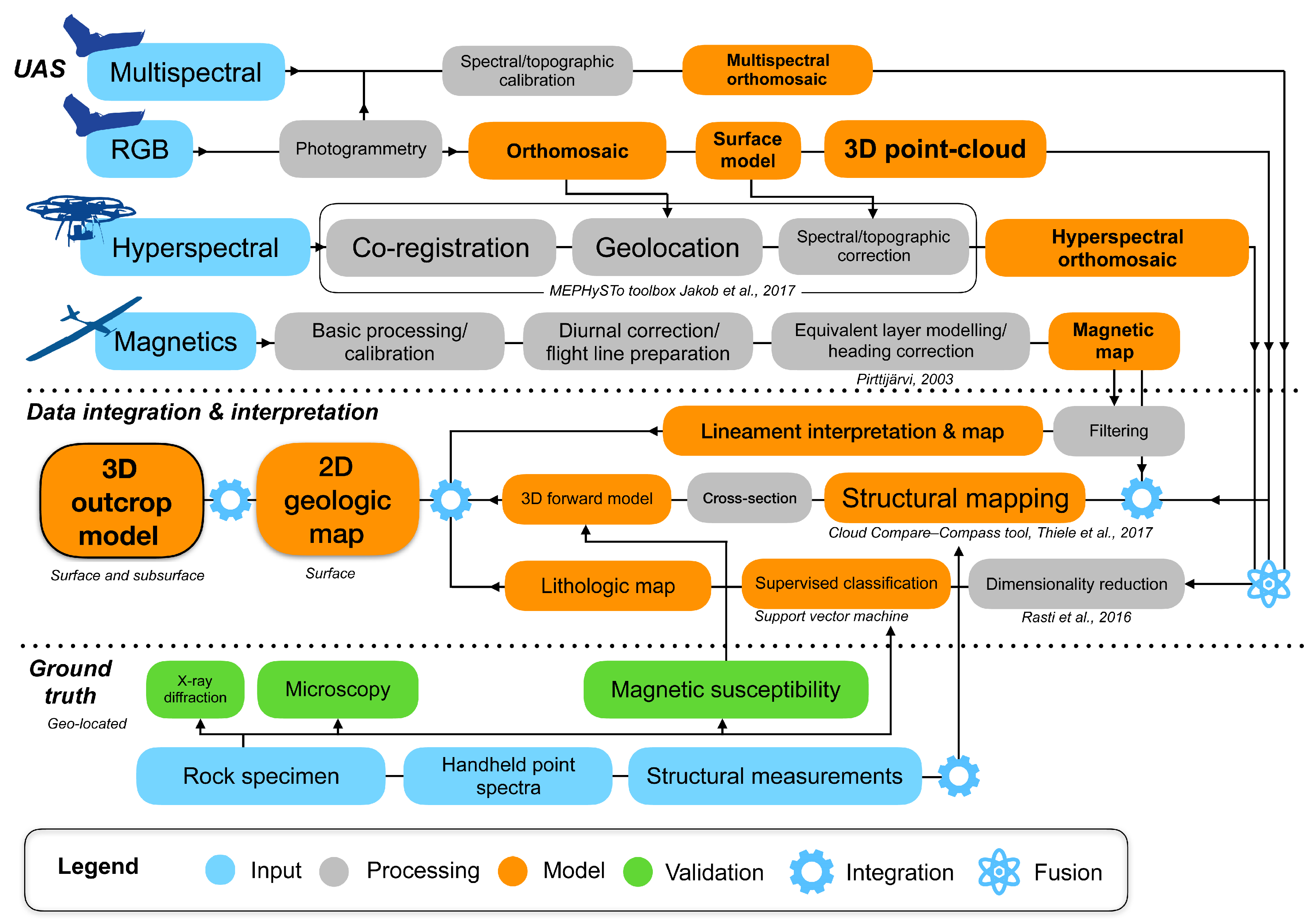
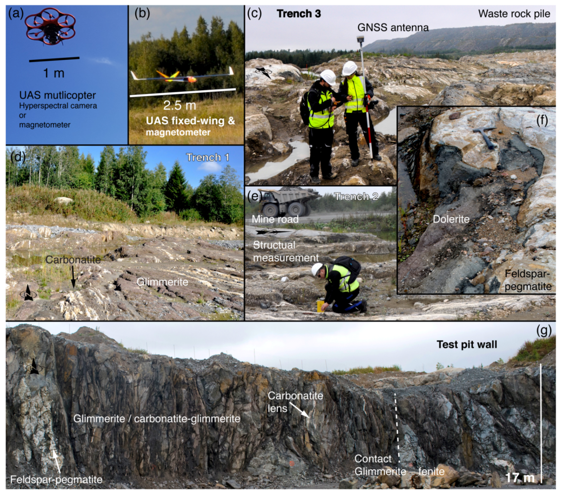
2.1. UAS Data Acquisition Method

We collect RGB and multispectral images (MSI) with a fixed-wing UAS. Structure-from-motion multi view stereo (SfM-MVS) photogrammetric workflows allow us to construct a digital surface model and an orthomosaic from RGB and MSI orthophotos. RGB information, that provides the highest spatial resolution, is used to identify geological structures. MSIs provide additional spectral information compared to RGB images, and a much larger footprint than hyperspectral image (HSI) data in this acquisition setup. All images are geotagged from the drone’s onboard GPS. Images are rectified using a number of ground control points.

The resulting SfM-MVS digital surface model (DSM) is used for topographic correction and referencing of the HSIs, and for structural analysis. By means of CloudCompare (www.danielgm.net/cc, vers. 2.11) and its Compass tool plugin [35], we semi-automatically trace and define best-fit planes for faults, foliation, and lithologic contacts directly on the point cloud. For ambiguous areas, supporting UAS data layers (e.g., HSIs, magnetics) are re-examined in the 3D environment.

We acquire UAS-based hyperspectral data frames with pre-coded flight paths in stop-and-go mode along the outcrop to maximize UAS surface coverage. We employ UAS-borne frame-based cameras because of their advantage in creating full image frames which, in our experience, are inherently less distorted than push-broom scanner data. For all HSI data, we manually crop water bodies and non-geologic structures such as roads and vegetated zones from the mosaics, or use semi-automatic masking with a spectral vegetation index.

We conduct UAS-based magnetic surveys using a fixed-wing drone to collect a high-resolution magnetic data set over the survey area, using predefined flight plans. Subsequently, we apply standard magnetic interpretation methods to inspect the shape and dimensions of the measured magnetic anomalies. The analytic signal or total gradient amplitude method [36] is utilized to estimate the location and depth of anomaly sources, as this function is independent of source magnetization direction [37]. Furthermore, we compute the first vertical derivative from total magnetic intensity (TMI) data to enhance the magnetic anomalies and reduce residual influences [38].

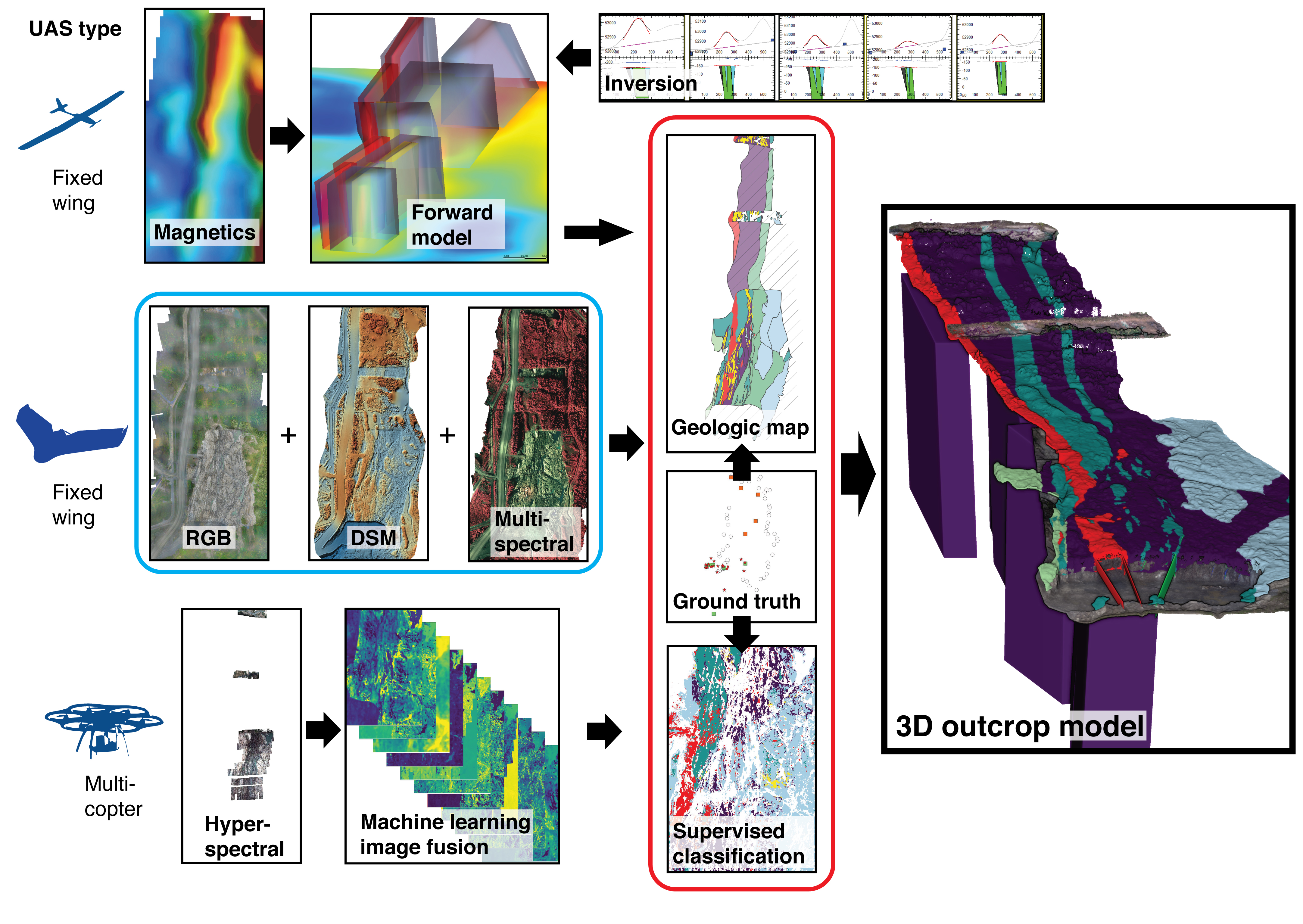
2.2. Data Products: Feature Extraction, Supervised Image Classification and Magnetic Forward Modeling

We perform data fusion on a “noisy” outcrop to reduce ambiguity of interpretation while increasing detection confidence and accuracy of classifications [39]. The feasibility of such a fusion approach was laid out for different lithologies at laboratory scale where multi-source hyperspectral and photogrammetric techniques were combined [40]. We apply spatially constrained feature extraction on the UAS-based optical imagery for a consistent classification as part of our multi-sensor data approach to enhance image classification results. The orthogonal total variation component analysis (OTVCA) is used to reduce data dimensionality [41]. It optimizes a cost function to obtain the best representation for multi-layer image data in lower-dimensional feature space, while giving a spatial smoothness over local neighboring pixels by minimizing the total variation of the image signal. OTVCA is robust towards non-systematic, random noise (e.g., salt-and-pepper noise) and has increased weight on neighboring pixels during the dimensionality reduction [42].

For supervised image classification, we choose the support vector machine (SVM) algorithm with Gaussian radial basis function (RBF) kernel, using the library for support vector machines (LibSVM) toolbox [43]. RBF-SVM is proven to perform well with heterogeneous classes and sparse training data, both of which are common cases in geological mapping [42]. Training and validation samples or pixels are defined by selecting pixel aggregates from the HSI data in a GIS environment from points with defined lithologies. The number of training/validation classes varies according to our field observations of the local lithologies.

For a 3D integration and interpretation of our UAS magnetic data, we use forward modeling. Model geometries are established by the UAS-based orthoimagery, hyperspectral mosaics and the DSM. The photogrammetric 3D outcrop model and ground measurements provide constraints on strike/dip and azimuth of the source bodies. Magnetic susceptibility values assigned to the modeled bodies are taken from published literature [27,28,44] and from additional measurements collected with a handheld susceptibility sensor over selected rock samples.

2.3. The Adapted Workflow Conducted for This Survey

We summarize the main characteristics of used sensors here (

Table 1. Sensors with technical specifications and platforms used for experimental data during this study.

Senor Type/Carrier Platform	Sensor	Resolution Spatial/Spectral	Bands/Sampling Range/Frequency	Data Product
Snapshot camera/Fixed-wing UAS	Parrot S.O.D.A.	5472 × 3648/ –	3/RGB/0.3 Hz	Orthomosaic-RGB, digital surface model
Snapshot camera/Fixed-wing UAS	Parrot Sequoia	1280 × 960/10–40 nm (FWHM)	4/550–790 nm/0.3 Hz	Orthomosaic multispectral
Frame-based camera/Multicopter UAS	Senop Rikola	1010 × 648/8 nm	50/504–900 nm/manual	Orthomosaic hyperspectral
Three-component fluxgate/Fixed-wing UAS	Radai magnetometer	– /0.5 nT	1/±100,000 nT/10 Hz	Magnetic raster grid

) and for specific technical details of our UAS workflow and data acquisition, we refer to Appendix A and [24].

We used the senseFly eBee Plus fixed-wing (www.sensefly.com, senseFly, Cheseaux-sur-Lausanne, Switzerland) equipped with either a high-resolution RGB camera (www.parrot.com, Parrot S.O.D.A., Parrot SA, Paris, France), or a multispectral camera (Parrot Sequoia). Processing of RGB and multispectral drone-based data was conducted in Agisoft Photoscan (vers. 1.4, Agisoft Ltd., St.Petersburg, Russia) following recommended protocols [45,46].

Our used hyperspectral frame camera was the Senop Rikola hyperspectral imager (www.senop.fi, Senop, Oulu, Finland). The camera was stabilized by a gimbal (roll and pitch axes) and transported on board of the Aibotix Aibot X6v2 multicopter (www.leica-geosystems.com, Leica Geosystems, Heerbrugg, Switzerland). Automatic HSI georeferencing, mosaicking and application of topographic corrections (c-factor method) on each HSI scene based on the photogrammetric DSM was conducted after Jakob et al., 2017 [47]. We applied the empirical line method [48] to convert the images from radiance to reflectance units, using ground calibration targets.

Magnetics were flown with a composite material fixed-wing UAS Albatros VT2 from Radai Oy (www.radai.fi, Radai Ltd., Oulu, Finland). This UAS utilizes a three-component fluxgate magnetometer, a cost-reducing drone-based sensor [49], attached to the drone’s tail boom. With 2.5 m of wingspan and a flight endurance of roughly 3 h, it can easily cover outcrops at square kilometer scales. The survey was flown with traverse lines at 30 m spacing, 99.4⁰ azimuth and tie lines at 60 m spacing and 9.4⁰ azimuth. The fixed-wing follows the topography along the flight plan based on any available high-resolution digital elevation model. In this case, we used publicly available data from the National Land Survey of Finland.

Magnetic data processing involved removal of spikes and duplicate points, compensation of the fluxgate magnetometer, computation of the total magnetic intensity from the compensated component magnetic data and removal of diurnal effects. Position coordinates, time stamps, barometric pressure and the three-component magnetic data were recorded simultaneously by data logging hardware. An equivalent source algorithm (equivalent layer model (ELM) after [50]) was utilized to prepare the final TMI grid for the survey with the minimum curvature gridding method of ELM data at 15 m cell size. The software Model Vision (vers. 16.0, Tensor Research Pty Ltd., Greenwich, Australia) was used for subsequent forward modeling. Five magnetic profiles crossing along the E–W direction on top and near the main trenches were used in the forward model. A number of simplified bodies with tabular geometries were modeled until a reasonable root mean square error (3–5%) between the measured and synthetic TMI response was achieved.

Covering the known lithologies, ground sampling locations of rock specimens (n = 23) and ground control points (n = 19) were localized with a Trimble global navigation satellite system (GNSS) kit (Trimble R5 base station, Trimble R10 rover; Trimble Inc., Sunnyvale, USA). An overview of the complete workflow is shown in Figure 1.

2.4. Ground Truthing and Laboratory Validation

Data integration at multiple scales, using local ground truth, airborne magnetics, and regional geology is an established method that can provide excellent results and meaningful geologic interpretations [51]. Our ground-truthing program involves rock sampling, as well as structural (n = 38) and spectral measurements (n = 336) and ground-based photogrammetry. All ground samples are geolocated using GNSS. All rock samples are cut and polished for optical investigation and some for analysis with selected geochemical and mineralogical methods.

We take several structural measurements (geological compass), which we incorporate in forward modeling of magnetic data. Main observations are made for contacts, orientation of dykes, and foliation.

During the outcrop studies, we record point representative spectra using a portable spectroradiometer in the available wavelength range of 400–2500 nm. We use selected scans as reference for the supervised image classifications (see Appendix A for point distribution and spectrometer specifications).

Laboratory validation methods, which represent traditional geological, mineralogical, and petrophysical verification methods, are selected to confirm our field observations, and to extract further geologic information from the study site itself. All measurements are conducted on collected rock specimens in the laboratory. Thin section samples are created from specimens covering all main lithologies of the outcrop and examined with optical and polarized light microscopy. Magnetic susceptibility and X-ray diffraction analysis is applied on selected samples (see Appendix D for additional information).

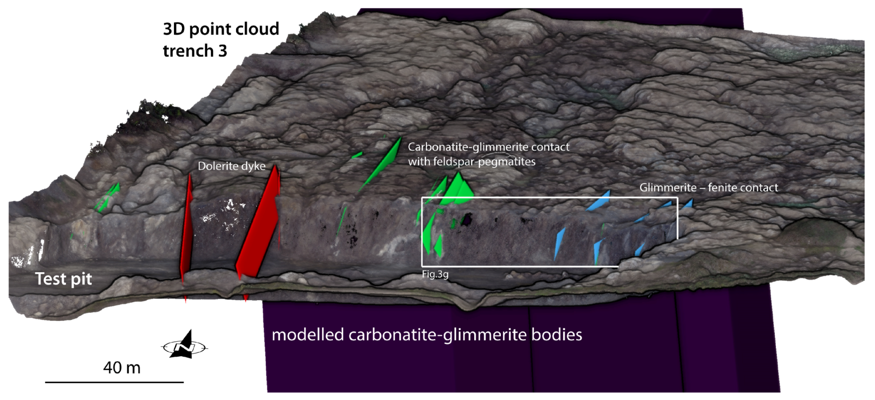
3. Case Study: The Siilinjärvi Carbonatite Complex

Here, we introduce the test area together with the geology. The Siilinjärvi carbonatite complex is situated 20 km north of the city of Kuopio in central Finland and extends for 16 km in N–S and 1.5 km in E–W directions (Figure 2a), with an estimated depth of 800 m [27]. It is one of the oldest known carbonatites with an Archean age of 2.6 Ga±10 Ma, according to U-Pb zircon dating [52]. The Siilinjärvi mine extracts carbonatite–glimmerite-hosted apatite ore for fertilizer production as one of the biggest producers in Europe.

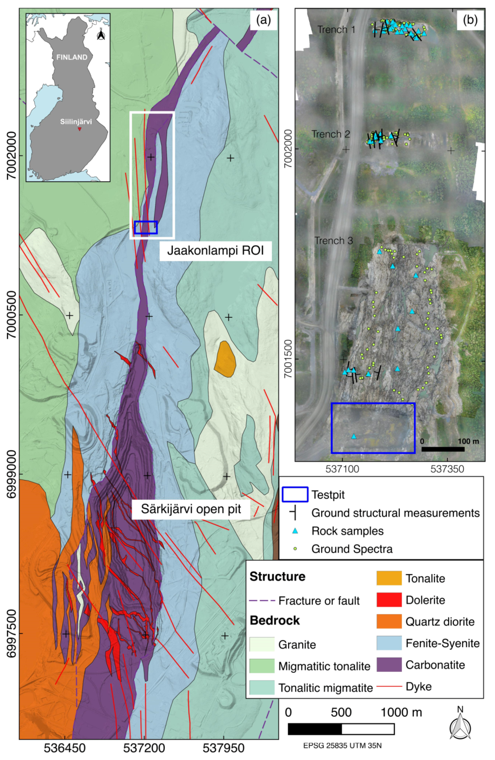
3.1. Local Geology and Study Area

The carbonatite intrusion was emplaced into basement gneiss and deformed by the Svecofennian orogeny at 1.8 Ga [53]. Local rock types are fenite, gneiss, carbonatite–glimmerite, diabase, and other dykes (e.g., local diorites). The central carbonatite–glimmerite ore body has a tabular form, is up to 900 m in width, and is surrounded by a fenite margin created by carbonatite-derived alkali metasomatism of the granite–gneiss country rock and syenite [54].

Brittle and ductile deformation caused structural segmentation of the carbonatite complex and surrounding rock, expressed as sharp boundaries within some areas of intermixed diabase, fenite, tonalite and carbonatite–glimmerite. Fenites as metasomatic products of diorite and gneiss are found in the magmatic contact zones between country rock and carbonatite–glimmerite [25]. This halo of fenitized rocks contains microcline, orthoclase, amphibole, and pyroxene, as well as carbonate, zircon, and quartz.

Several generations of mafic dykes (dolerite) cut the Siilinjärvi intrusion in NW–SE and NNW–SSE directions, with widths ranging from centimeters to meters [54]. Most of the dykes are steeply dipping and, depending on their generation, were subjected to deformation [31]. Sheared feldspar-rich pegmatite dykes with widths varying from 1–50 m were recently discovered by a large-scale drilling program in the Jaakonlampi area [55] and are exposed on the surface. Structural emplacement of the dykes is still not fully understood, but given their size and increased magnetic susceptibilities, they could be an important component of forward modeling.

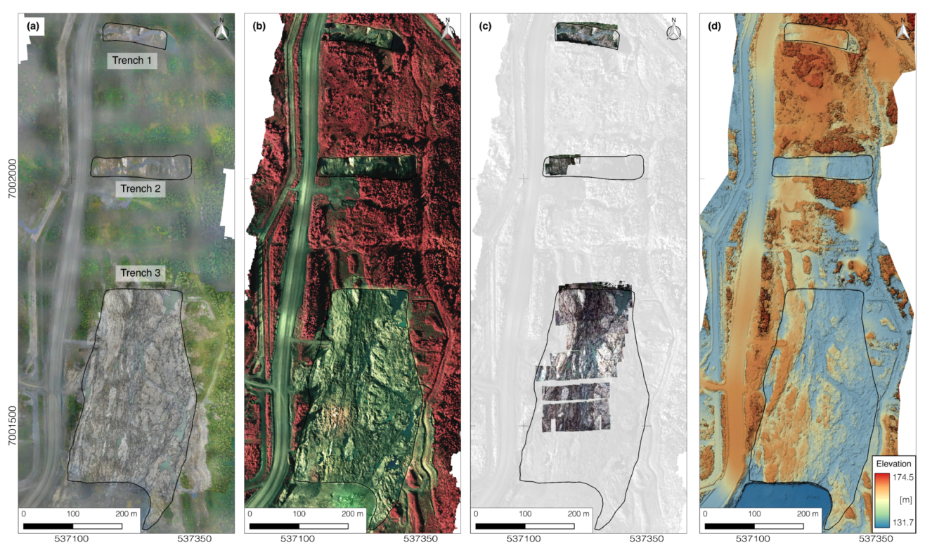
3.2. The Jaakonlampi Test Area

Situated 1.2 km north of the Särkijärvi main pit, the Jaakonlampi area (Figure 2b) provided the test zone for our UAS survey. Jaakonlampi extends ~1 km in the northern direction and is characterized by three distinct exploration trenches, which from north to south, henceforth we refer to as trench 1, trench 2, and trench 3. The mine company expanded the exploration program for trench 3 in 2018 and removed significant soil overburden, uncovering a large exploration trench (Figure 3c). However, the recent uncovering resulted in some remains of sand and clays on top of trench 3’s surface, challenging subsequent image classifications.

Within the glimmerite, the carbonatite is featured as thin, sub-vertical veins. The composition of carbonatite is mainly calcite, apatite (1.4–2.3 vol.%,) and magnetite (1 vol.%). On average, the ore contains 65% phlogopite, 19% carbonates, 10% apatite, 5% richterite, and 1% accessories that are mainly magnetite and zircon [54]. The composition of the three trenches (Figure 3c–f) is similar to the general configuration of the Siilinjärvi deposit. The southern-located trench 3 connects seamlessly to a so-called test pit (Figure 3g), an outcrop wall which presents a vertical geologic cross section of the lithological units further used in this study:

• Carbonatite–glimmerite (CGL) and carbonatite (CRB)
• Dolerite (DL)
• Felspar-rich pegmatite veins (FSP-PEG)
• Fenite (resp. syenitic fenite or fenite-syenite) (FEN-SYN)
• Glimmerite (GL)
• Granite–gneiss (GRGN)

4. Results

We present the mapping results sorted by method. Survey conditions, camera settings, and technical UAS-related data are found in Appendix A (

Table A1. Properties of test trenches, information for the UAS surveys, and further details of the HSI mapping, as we only surveyed the exposed trench rocks by HSIs. Altitude in m above sea level. The last column refers to the input layers used in the OTVCA for supervised image classification. GSD = ground sampling distance.

Outcrop/Method	Coordinates	Dimension x-y	Survey Condition	Used Bands/Integration Time	Flights/Coverage	GSD	Altitude	OTVCA Layers
Method(Hyperspectral only)
Trench 1	63.147N, 27.738E	130 × 36 m	sunny, windless	50/10 ms	1/5500 m2	2.7 cm	40 m	HSI
Trench 2	63.145N, 27.738E	200 × 40 m	sunny, windless	50/10 ms	1/3050 m2	2.3 cm	30 m	HSI
Trench 3	63.141N, 27.738E	220 × 400 m	low clouds, breeze	50/30 ms	3/38,200 m2	3.4 cm	50 m	HSI, MSI, RGB
Multi-spectral	63.143N, 27.738E	450 × 1430 m	sunny, windless	4/automatic	1/0.649 km2	10.5 cm	100 m	–
RGB	63.143N, 27.738E	540 × 1290 m	low clouds, breeze	3/automatic	2/0.623 km2	2.7 (1.5) cm	100 m/70 m	–
Magnetic	63.143N, 27.738E	620 × 1100 m	sunny, windless	–	1/0.695 km2	30 m *	40 m	–

* 15 m after interpolation.

). All trenches and the forested areas in between were surveyed by high-resolution RGB and multispectral UAS images and UAS magnetics. Additional hyperspectral imaging covers trench 1 completely, the western half of trench 2 (the other half was submerged by water), and the northern half of trench 3. Visual observation of the test pit wall showed dipping bodies between 70–90°, broadly striking along N–S.

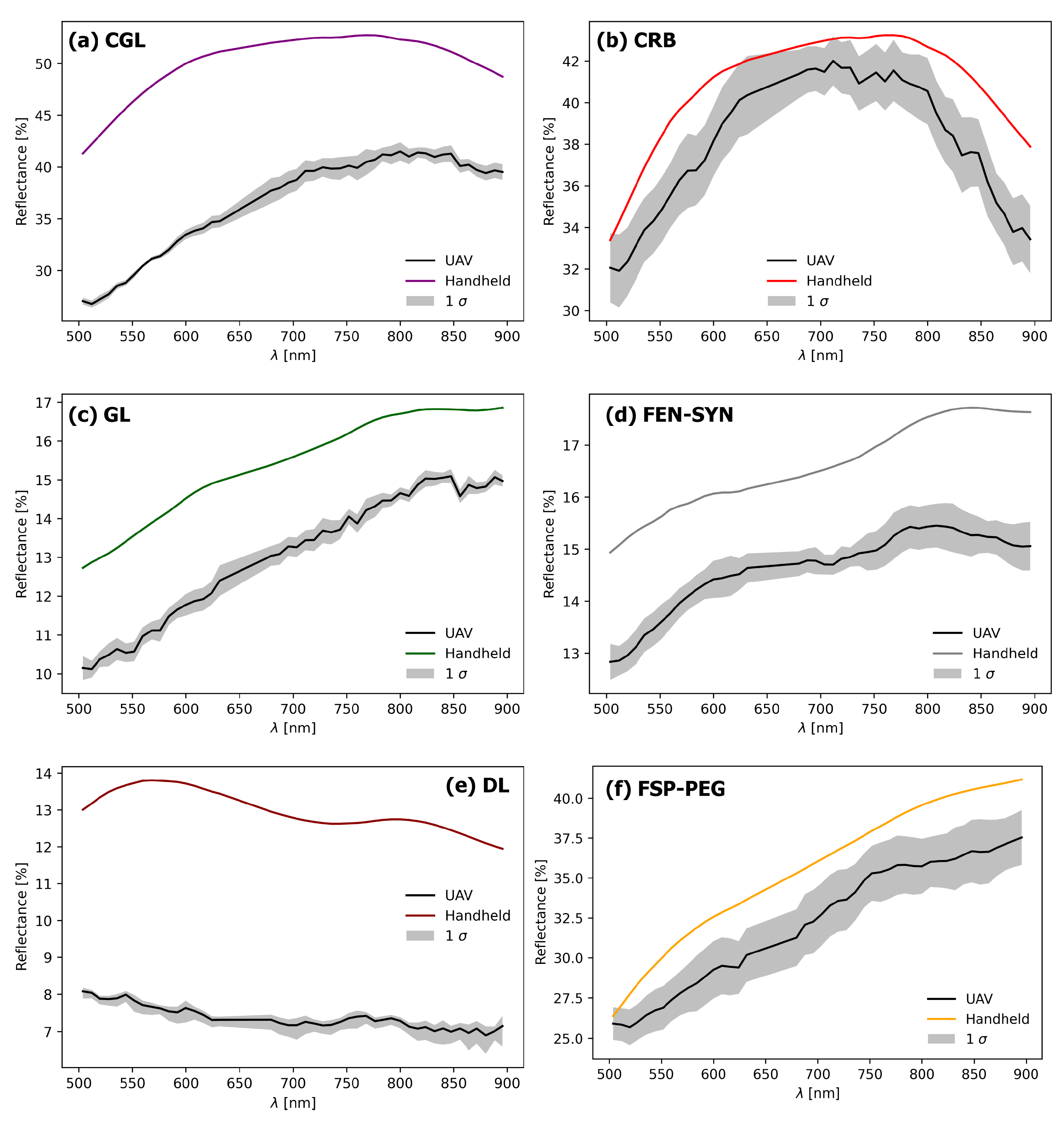
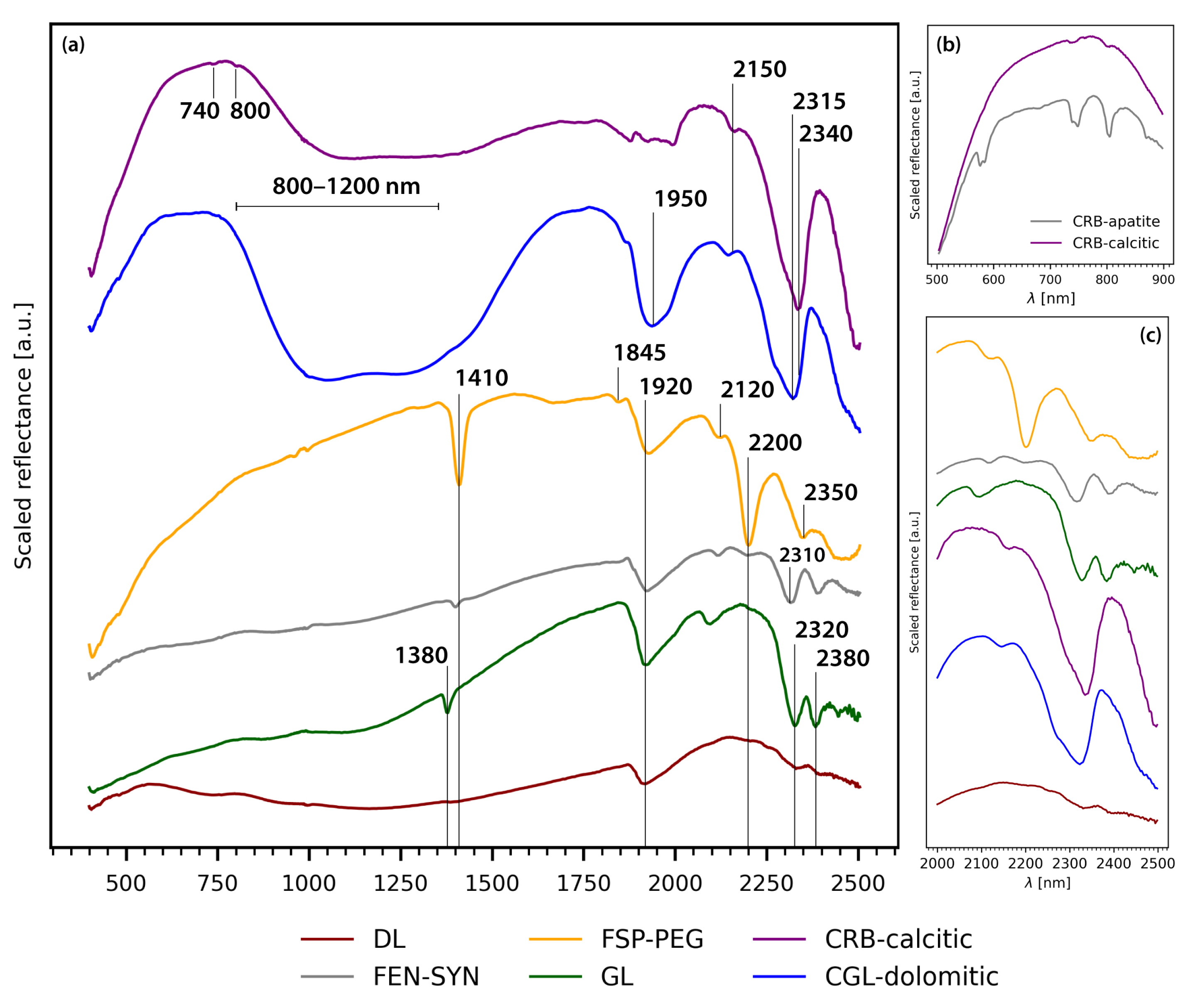
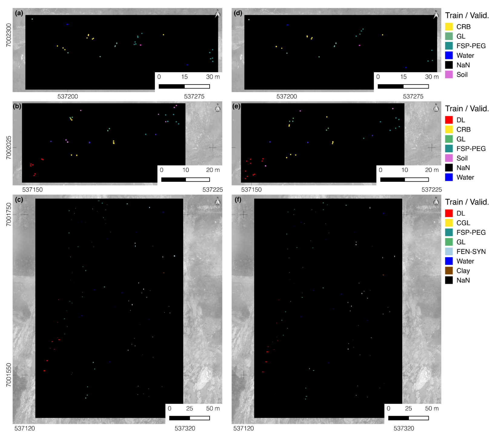
4.1. Ground Spectroscopy and Principal Lithologic Representation

We measured the three trenches in situ with a representative dense spectral point sampling campaign (Figure 2b) at trench 1 and 2 (275 locations). For trench 3, we conducted a broader sampling sweep (61 locations, 37 of those covered by UAS-based HSIs and MSIs). While understanding the spectral differences of the lithologies, we selected training samples for the supervised classification (Figure 1, last row) guided by the ground spectra (representative spectra in Figure 4), the RGB mosaic, and the OTVCA layers.

A relatively broad absorption between 900~1200 nm is attributed to the Fe²⁺ content in calcite and dolomite-rich carbonatite [56]. We detected rare earth element (REE) related absorptions at 580 ± 10 nm, 740 ± 10 nm, and 800 ± 10 nm (Figure 5b) [57]. A spectral shift from calcite-rich to dolomite-rich carbonatite is visible in our point scans, at the spectral minima transition from 2320 nm to 2340 nm (Figure 5c), related to vibrational processes of CO₃ combinations and overtones [58,59]. For glimmerite spectra, rich in phlogopite and biotite, we observe characteristic OH^- features at 1380 ± 10 nm and Mg-OH vibrational bands at 2320 ± 10 nm and 2380 ± 5 nm [58]. Carbonates are likely to influence the position of the absorption minima here. Hydroxyl group absorption features are seen for fenitized syenite spectra at 2315 nm and 2385 nm. Dolerite spectra show the lowest overall reflectance, weak Fe²⁺/Fe³⁺ charge-transfer absorptions at 800 nm [60] due to iron alteration but a prominent absorption at 1920 nm (OH^- related). Feldspar-rich pegmatites, expressing a larger spectral variety and incorporating Fe²⁺ and pronounced OH^- features are found at 1410 nm, 2200 nm (Al-OH), and 2350 nm (Mg-OH). We observed apatite in carbonatite–glimmerite rock samples as a possible proxy for REE occurrence.

4.2. UAS-Based Optical Remote Sensing Observations

The RGB orthophoto (Figure 6a), the MSI mosaic (Figure 6b) and the HSI mosaics (Figure 6c) provide first-order information for subsequent interpretation. Low ceiling clouds were present during the RGB acquisition flight, producing horizontal gray stripes in the data. Occasional leftover dirt patches reduce the spectral quality in some HSI scans of trench 3. Topographic expressions are seen in the UAS-based DSM (ground sampling distance 10.6 cm; Figure 6d). The eBee RGB and MSI orthomosaics envelope the complete rock outcrop extension, which is covered by vegetation stripes between trenches 1 and 2 and between trenches 2 and 3. HSI mosaics were acquired completely for trenches 1 and 2. Trench 2 was partly covered with water on large surface portions. Low illumination conditions during the HSI acquisition of trench 3 reduced the spectral quality for all scans there. We augment the data set of trench 3 by using two additional data layers (DSM, MSIs) from the area. Those additional layers were resampled to the common lowest resolution (from the DSM) and fused with the HSI data set before applying the dimensionality reduction by OTVCA to improve supervised image classification.

The OTVCA-based false-color band combinations we selected for high variations are shown in Figure 7a,b. Only the merged multi-sensor OTVCA bands for trench 3 (Figure 7c) contain MS, RGB, and DSM data. Fusing those additional data layers for the classification of trench 3 helped to close some data coverage gaps of the hyperspectral survey (Figure 7c). The final classification produced by the SVM classifier and visual inspection was used to create the surface geology map. The resulting overall accuracy (OA) for all three trenches (>90% OA each) is acceptable. Overall supervised classification accuracies with used ground truth are as follows in mean accuracy (MA), OA, and kappa coefficient (κ): trench 1—MA 96.5, OA: 95.3, κ: 0.94; trench 2—MA 91.0, OA: 90.0, κ: 0.88; trench 3—MA 95.3, OA: 95.3, κ: 0.95. We refer to Appendix A for visualized training and validation samples, as well as confusion matrices per trench classification.

Although we achieved high classification accuracies, three falsely classified zones are identified (Figure 7f), i.e., a large block of carbonatite (25 m length) in the fenitized syenite and a stripe of dolerite extending into the feldspar–pegmatites and the mine road.

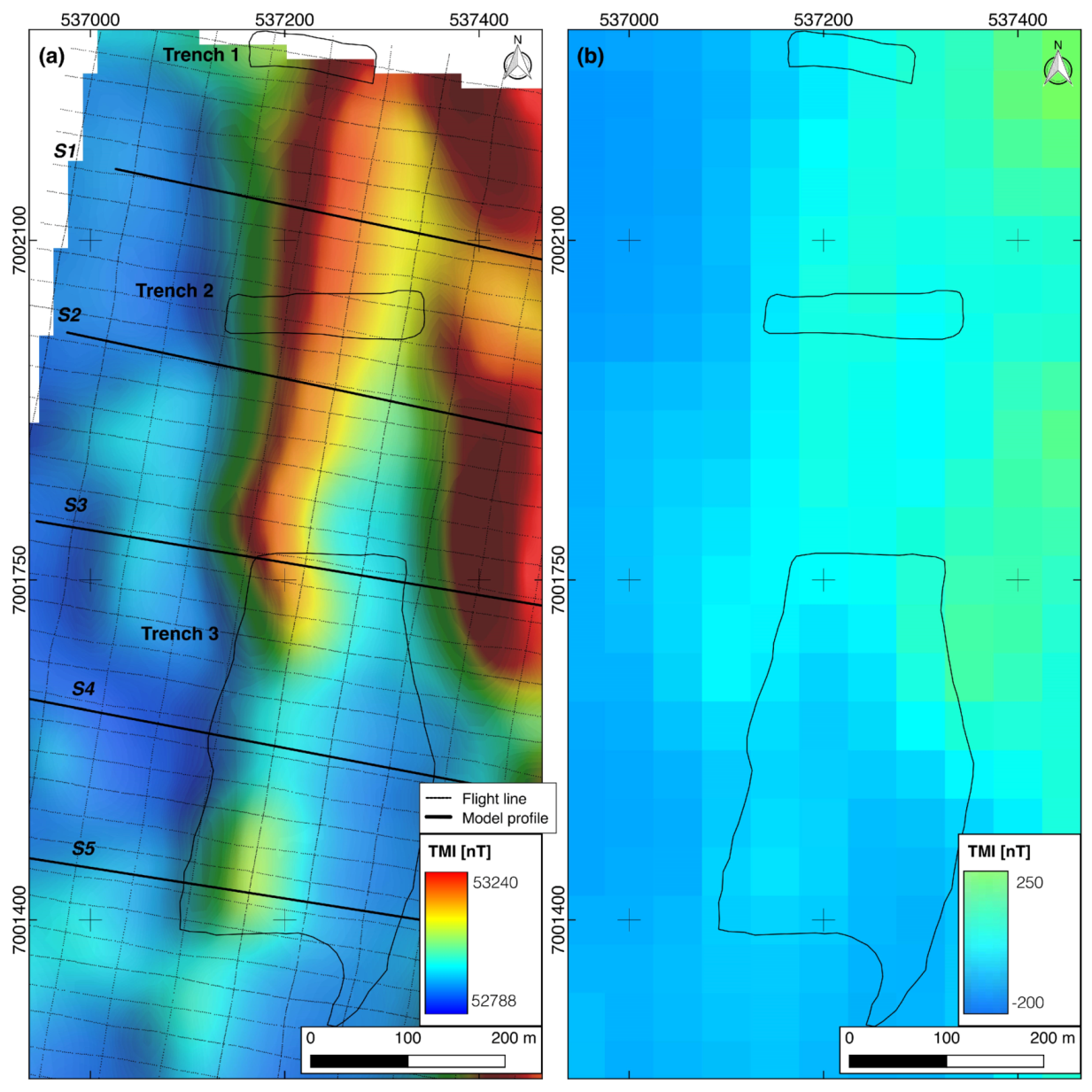
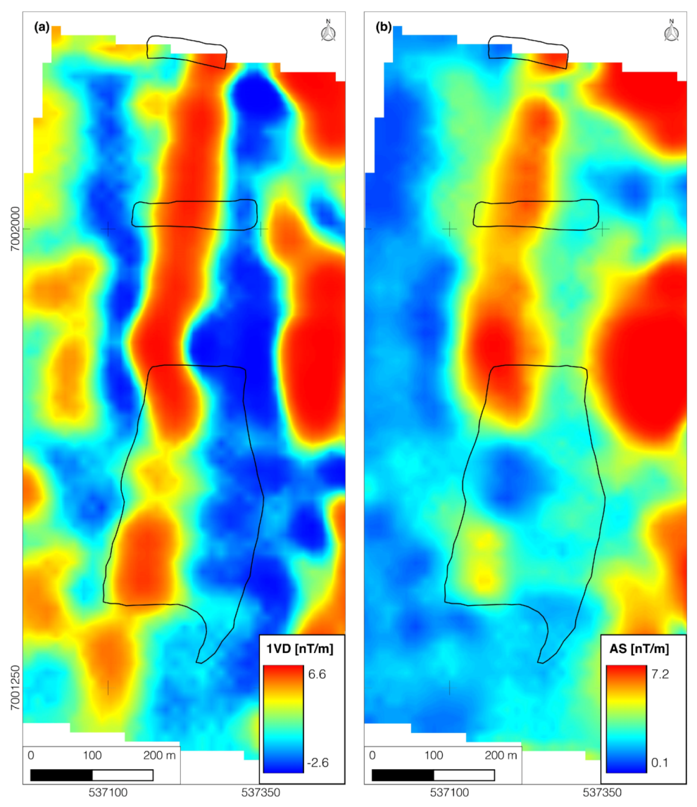
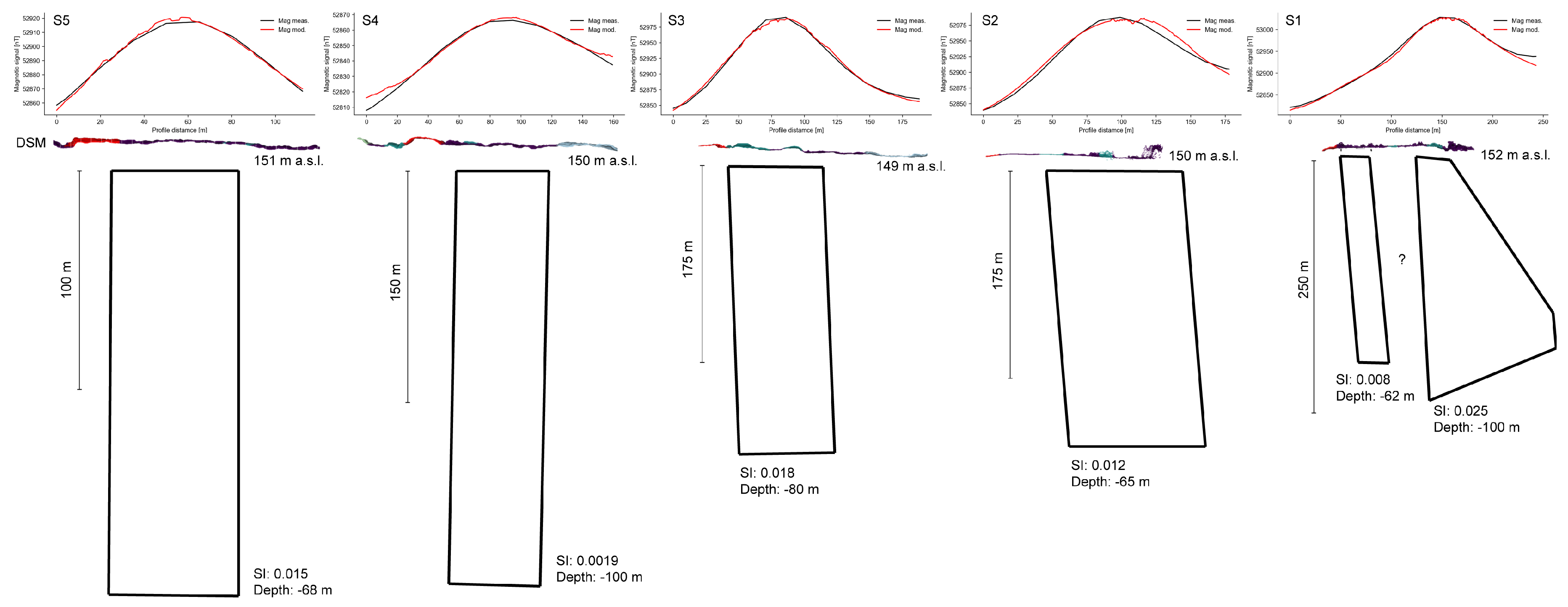
4.3. UAS-Based Magnetic Observations

Magnetic data interpretation is based on the processed TMI (Figure 8a) and filtered data products. The total survey length was ~ 39 km, with a mean flight height of 48 m above sea level (a.s.l.), a sampling line point distance of 2.1 m, and a mean velocity of 17.7 m/s. We show regional airborne magnetics ([61] modified after Geologic Survey of Finland © 2016) for comparison (Figure 8b). The regional field shows a decreasing tendency towards the west. A pronounced magnetic anomaly, with values reaching 400 nT, is heading in the north to south direction. At the center of trench 3, the TMI trend is decreasing. A TMI field strength reduction is visible at the southern end of trench 3 above the vertical wall of the test pit.

The first vertical derivative (1VD, Figure 9a) sharpens the edge of the N–S trending anomaly and the 1VD outlines the distinct transition from low to high TMI values, which we interpreted as possible lithologic contact between country rock and fenite. By using the analytic signal (AS), which serves to minimize the impact of any magnetic remanence on the observed magnetic anomaly pattern, we enhance magnetic contacts, interpreted here as carbonatite–glimmerite and country rock (Figure 9b). Based on the aforementioned image classification (Figure 7f), the western border of the dolerite unit could be traced, which is running from N–S through the whole study area. A decrease in the vertical gradient magnitude is seen again in the center of trench 3, where the shear zone is located (Figure 2 and Figure 9) [55]. The spatial width and field strength of the central anomaly could be related to the volume of material replaced by the non-magnetic feldspar-rich pegmatite dykes. The magnetic low at the center of trench 3, starting 50 m north from the test pit, is measured atop the observed fold and shear tectonics, where magnetic minerals are altered, displaced, or destroyed [62]. The two spatially large, oval-shaped anomalies cross above the eastern map border of Figure 8a.

4.4. Geologic Modeling and Ground Magnetic Susceptibility

Magnetic susceptibility measurements are imperative for a supporting forward model as a secondary data derivative, based on UAS magnetics. The susceptibility ranges of our sampled lithologies are aligned with values presented in the literature and our own sampling.

Table 2. Augmented value range for magnetic susceptibilities based on reference literature and own measurements, values given in SI units.

Lithology	Almqvist et al., 2017 [44]	V. Laakso, 2019 [28]	Measured	Used
Dolerite	1.26 × 10−4 – 1.29 × 10−3	1.0 × 10−2 – 1.6 × 10−1	7.0 × 10−4 – 1.35 × 10−2	1.0 × 10−5 – 1.7 × 10−2
Carbonatite–Glimmerite	4.27 × 10−4 – 2.09 × 10−1	1.3 × 10−1 – 2.1 × 10−1	1.0 × 10−4 – 1.1 × 10−2	3.2 × 10−3 – 2.5 × 10−2
Feldspar–Pegmatite	–	0 – 5.0 × 10−4	7 × 10−5 – 1.4 × 10−4	1.0 × 10−5 – 5.0 × 10−4
Fenite	–	1.3 × 10−1 – 1.5 × 10−1	1 × 10−6 – 1 × 10−5	–

lists susceptibility ranges for the relevant lithologies.

We constructed a model, starting with simple cuboidal geometries, and advanced to polygonal tabular sheets, with their surface geometry constrained by our UAS-based surface geologic map (Figure 10). UAS-based DSM data were used to constrain the top surface of each polygon. An approximate maximum depth of 250 m meters was imposed, based here on available literature information for the study area. Body geometry (strikes and dip, width, azimuth) were taken from photogrammetric interpretation and compared with our own ground measurements. Initial susceptibility values were assigned to geological units on the basis of the literature and measured susceptibilities (Table 2). Optimization of the model was achieved using the inversion tool provided with the ModelVision software. After continuous reiterations, a root mean squared error between synthetic and modeled TMI response of 3–5% was reached per profile. In our model (cross section in Appendix B) one implication could be that the dolerites we measured can reach magnetic susceptibilities close to carbonatite–glimmerite. Yet, this could be an observation at only some depth or related to shearing. The dolerites are known to be low or non-magnetic in the mine area (personal communication, Yara chief mine geologist). The modeling results are integrated in Section 5.1 with the surface data for the final mapping. Extracted body boundaries are used to refine the surface map in a 2D cross section depth map over trench 3 (Figure 10c).

5. Data Integration and Validation

In this section, we present the integrated results of our UAS mapping approach, bringing together data acquired with UAS platforms and ground survey. All analyses and maps were conducted and created in Quantum GIS (vers. 3.4, QGIS development team). The inferred lithologies between the outcrop trenches are mapped using the UAS magnetic observations. The following link to the integrated 3D model is available online at https://skfb.ly/6U6Xo.

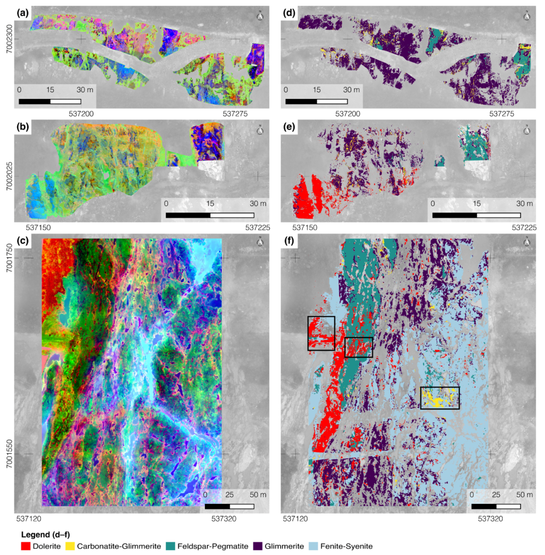
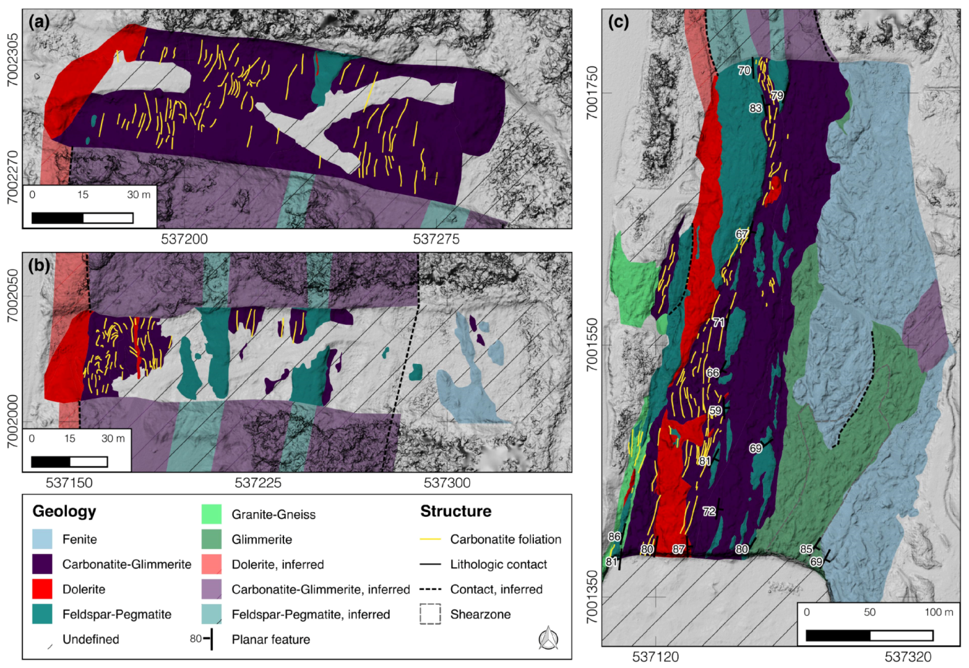
5.1. Geologic Mapping and Interpretation

Structural features (e.g., foliations, discontinuities, lineaments) and contours are interpreted visually in magnetic and DSM data, and with finer detail aided by the RGB orthophotos (Figure 8a). We produced magnetic contours from TMI, AS, and 1VD data. To do so, we calculated the contour lines from TMI and for filtered magnetics, to obtain magnetic isolines per data set in quartered data range steps and subsequently kept only each isoline representing the 50% data threshold. Thus, one isoline shows the arithmetic data threshold representing a mean. We observe that the TMI and 1VD isoline are superimposed along the western border of the main anomaly in the center of trench 3. This might reflect a well-expressed, deep contact of carbonatite–glimmerite and country rock. The ‘mag gradient’ outlines the observed field decrease (center of trench 3; Figure 9). The geologic surface interpretation (Figure 10b) brings together all data sources: RGB orthophoto, supervised classification of HSIs, and fused data. We extracted 66 discontinuities manually for the three trenches (sum of length: 4.46 km), with a mean length of 50 m per structure. We mapped a high density of features along trench 3, as a result of high contrast in both RGB and HSI mosaics. The visual overlap of RGB, HSIs, DSM and magnetics aided the extraction when contacts or boundaries were blurred or ambiguous. The shear zone in the south-east of trench 3 (Figure 10c) expresses visible lineament offsets and a dense fracture pattern in RGB data. We do not infer fenite as there are too few surface observations for reference, but the magnetics indicate a contact between carbonatite–glimmerites and fenites.

We infer that the lithologies carbonatite–glimmerite, dolerite, and feldspar–pegmatite continue their N–S trend and intersect with the surficial identified structures. A good example is the case for dolerite and feldspar–pegmatite, which we can observe for trenches 1 and 2 (Figure 10a,b compare observed vs. inferred lithologies). Additionally, we map the smaller carbonatite features based on HSI classifications and show them as overlaying foliation (Figure 11). A 3D representation of the pit wall is seen in Figure 12.

By applying the Cloud Compare compass tool [35], we could extract 21 contact planes between feldspar–pegmatite and glimmerite, 10 dolerite contacts, and 6 glimmerite–fenite contact planes, all of which were located in trench 3 (Figure 12). The largest dolerite dyke had a diameter of ~30 m. Trenches 1 and 2 expressed few topographic differences to extract meaningful contact planes.

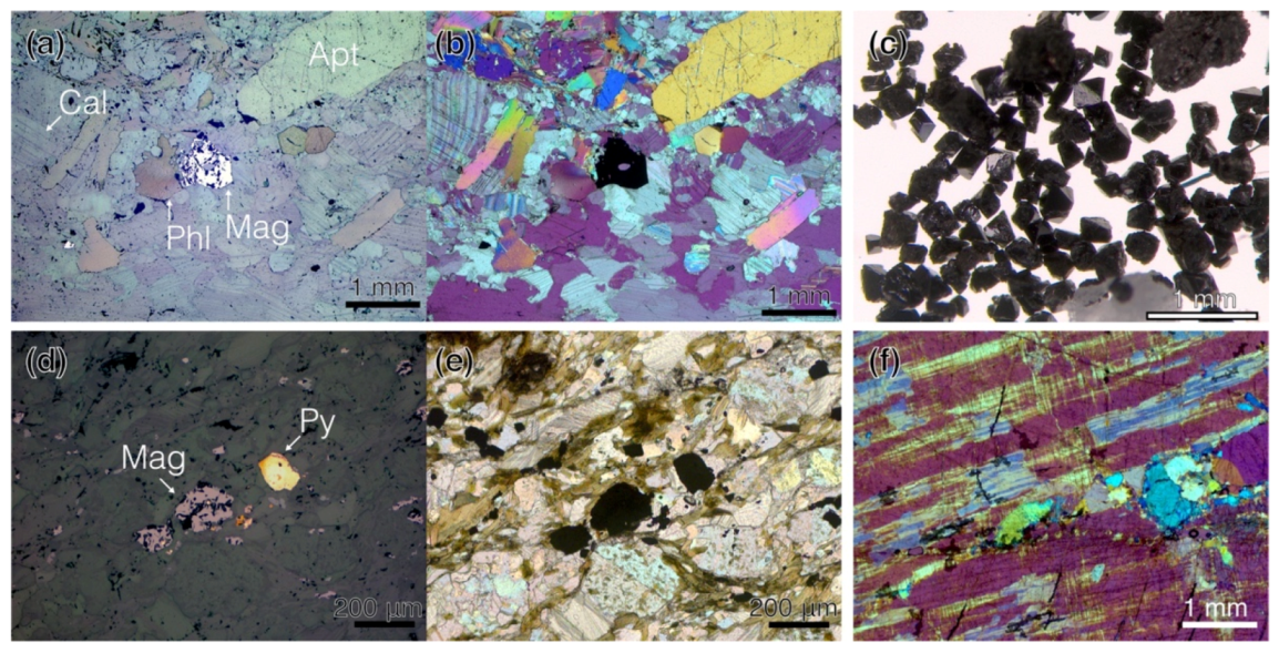
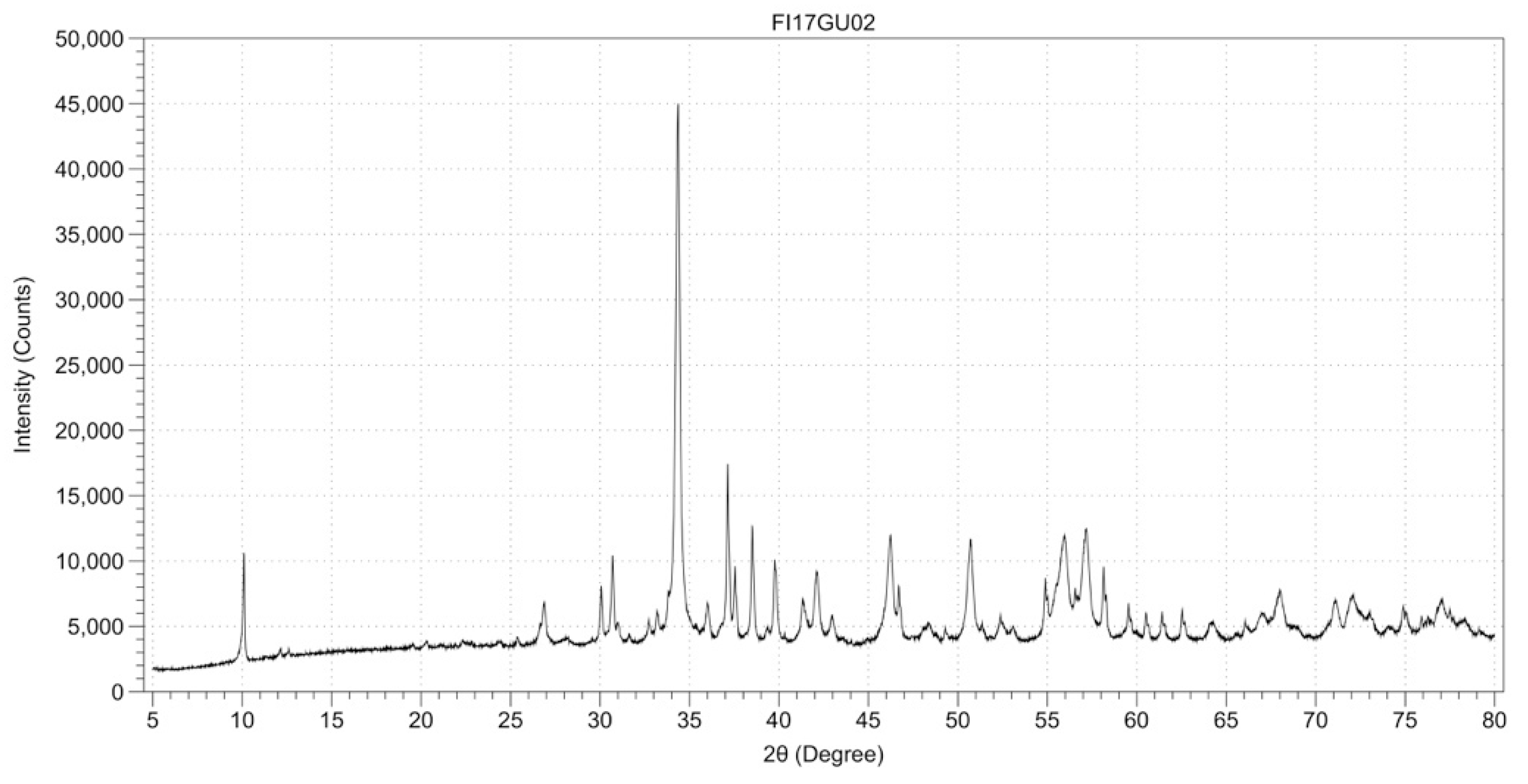
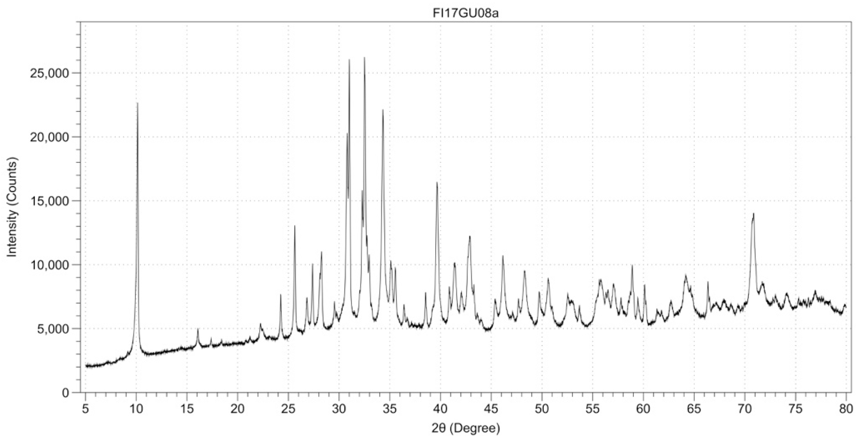
5.2. Mineralogic Validation and Additional Observation

We deployed optical microscopy (Appendix C) and X-ray diffraction (XRD) methods for mineralogical analysis. The microscopy of carbonatite–glimmerite shows calcite, a homogeneous distribution of magnetite grains ranging in size from microns to millimeters, and larger pyrite crystals. We observed idiomorph magnetite in rock thin sections of carbonatite–glimmerite, glimmerite, and dolerite. Magnetite seems to be in co-occurrence with pyrite. Combining microscopy and XRD, we detect some presence of magnetite in several mapped carbonatite–glimmerite and glimmerite units of this study. XRD of a bulk handheld specimen collected from carbonatite–glimmerite shows 1.8 wt.% of magnetite. Further evidence of magnetic minerals was only observed in one dolerite sample (2.4 wt.%). We did not identify magnetic minerals in the remaining lithologies from microscopy (fenitized syenite, feldspar–pegmatite). Moreover, XRD patterns detect calcite, apatite, biotite, pyrite, quartz, albite, ankerite, and actinolite (Appendix D).

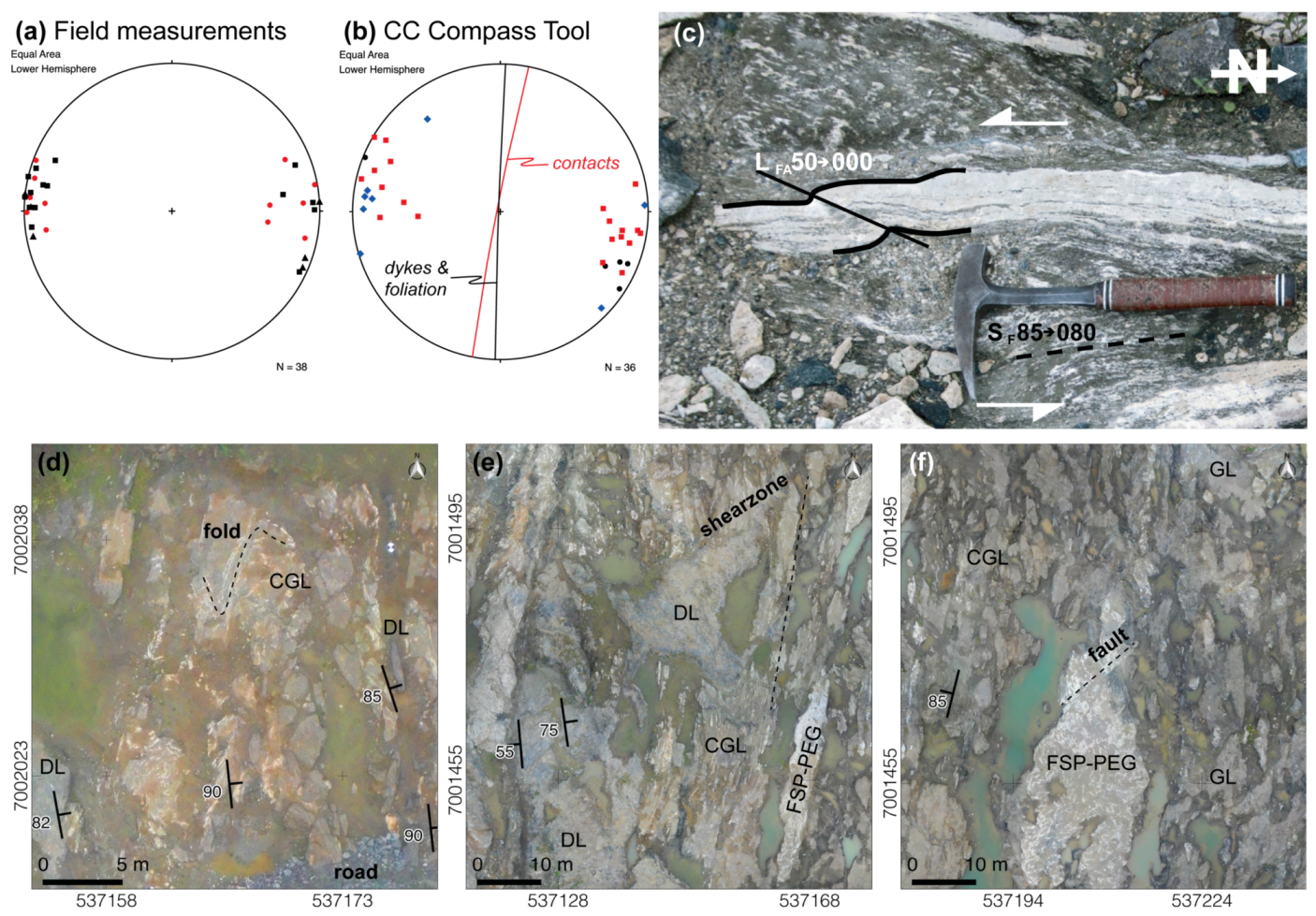
5.3. Validation of Structural Observations

The results of the digitally extracted structural measurements are summarized (Figure 13) and compared with the ground measurements. High image contrast and geometric expression were found at the test pit of trench 3, and therefore used for extraction. Thirty-two contact points, 6 foliations, and 2 dykes (carbonatite, dolerite) were measured in situ during the field campaign. Digital point cloud measurements of apparent large units were extracted mainly on the test pit wall for dolerite, carbonatite–glimmerite and fenite features. Twenty contacts between carbonatite–glimmerite and feldspar–pegmatite, 10 dolerite dykes, and 6 glimmerite–syenite–fenite contacts were extracted digitally. Our structural observations of the Jaakonlampi area show an N–S trend, which is consistent with the formerly described N–S striking foliation trend of the host rock [25], and shearing along the contacts of intrusions with host rocks [54]. Structural orientations of contacts, dykes and foliations are comparable in their main trends (Figure 13a,b,d). Smaller feldspar–pegmatite units (Figure 13e,f) were measurable along the carbonatite–glimmerite in trench 3. The rather flat surfaces, low topography and reduced RGB image contrast of trenches 1 and 2 could not provide sufficient contrast for usable structural measurements. NW–SE-oriented shearing affects structural expressions in our study area (Figure 13c). Several shearing events were identified in the Jaakonlampi area (four deformation stages with D1 || D3 identified in [55]). At the shear zone of trench 3, we observed contacts of carbonatite–glimmerite with granite–gneiss and an occasional absence of the fenite–syenite halo.

6. Discussion

6.1. Assessing the General UAS Survey Workflow with Focus on Image Data

We tested a survey approach that is only limited by the external conditions for UAS operations, such as weather and legislation. Our multi-sensor UAS toolkit aids geologic ground mapping, i.e., at around 1 km² [64]. Our combination of different UAS-based sensors fills spatial gaps during the survey, and provides a wealth of interpretable data. Extracted spectroscopic and magnetic observations complement each other to capture surface and subsurface information, which allows an integrated geologic interpretation. Furthermore, we expand the coverage of the survey area by complementing missing areas with data from other sensors.

As expected from our lithologies at hand, a full class distinction based solely on HSI and RGB data was not feasible at first. Here, sensor integration substantially improved the UAS-based supervised image classifications. Some lithological boundaries seen in spectral data are expressed in the DSM topography. For example, classification accuracy for the feldspar–pegmatite intrusion and dolerite contacts was improved by including the DSM layer in the OTVCA feature extraction of trench 3, because those lithologies are more extruded. Particularly for trench 3, the occasional clay–soil patches smear larger surfaces and the cloudy weather during this data acquisition made it worthwhile to include additional information. OTVCA takes spatial relationships of multi-dimensional data (i.e., dozens of image channels) into consideration. By optical inspection, the selection of 13–20 bands of each extracted OTVCA data set of the three trenches (equaling 20–30% of the provided number of input bands) for the SVM classifier was feasible. Optical inspection means here that OTVCA bands with obvious noise content (stripes, artifacts, contrast gradients) are discarded. With a careful selection of training samples, we obtained a classification in good agreement with geologic ground mapping.

The multicopter-based hyperspectral data could identify spatially small (~5 cm), spectrally pronounced anomalies, i.e., fine carbonatite lenses and is effective at the given outcrop dimension. The same lenses are visible in RGB, but cannot be distinguished spectrally, e.g., from feldspar–pegmatite rubble. Some lithologies (feldspar–pegmatite, fenite–syenite, granite–gneiss) are hardly discernable due to their lack of characteristic spectral features in the VNIR range. For example, average reflectance of fenite–syenite was similar or higher than for feldspar–pegmatite and granite–gneiss. However, we could still discriminate those rocks by using the machine learning-based spatially constrained feature extraction. OTVCA allowed us to pass not only spectral information, but also slight spatial, textural, or overall reflectance changes to the classifier. With a set of representative, well-defined training points, the classifier is able to assign meaningful labels even to classes lacking any indicative spectral features. While delivering a good classification performance, this approach is highly dependent on good-quality training data. UAS short-wave infrared (SWIR) sensors would add more confidence to the classification and allow a direct, spectroscopic analysis of a much wider range of mineralogical features, however, their pricing and weight is still an obstacle. Light-weight VNIR sensors in combination with advanced, open-source machine learning techniques, have been shown to offer a cheaper, but still reliable, alternative for the discrimination of known lithological domains.

Furthermore, we see a high feasibility when UAS spectroscopy is used for, e.g., iron oxides and rare earth element identification. Neodymium and dysprosium are promising targets for remote sensing studies [57]. We observed specific rare earth element-related absorptions in VNIR regions of handheld spectra in local apatite (Figure 5b). For mapping, we are particularly interested in spectral absorption of Fe²⁺ bands in the range of 800–1200 nm as a target for the HSI camera. Further CO₃ related absorption around 2330 nm, indicative for carbonate mineralogy (i.e., carbonatite), is only detectable in the SWIR range of handheld spectroscopy [65,66]. To assist with UAS magnetic mapping, first-order results from UAS-based RGB orthophotos are available directly after each flight (Figure 6a). Orthomosaics could be further used to optimize and refine magnetic flight plans in the field, if important anomalies are identified. While atmospheric conditions influenced the data quality acquired from optical sensors, the magnetics could be flown with a low cloudy ceiling or over wet surfaces without any disturbance. Line spacing, altitude, and sampling frequency of UAS magnetics define the features we can resolve physically, and therefore the size of targets we can model and interpret. We consider that the fixed-wing UAS probably created more valuable data for mapping with high surface coverage. Fixed-wing flight endurance was not exhausted with the current target area. In this case study, the following surface coverages were achieved per sensor:

• Magnetics: 0.695 km² (interpolated grid surface from 39-line km);
• MSIs: 0.649 km²;
• RGB: 0.623 km²;
• HSIs: 0.047 km² (sum of HSI flights).

The used UAS-fitted workflows are matured to a high user friendliness and could be flexibly adapted to all mining and exploration scenarios, where high resolution and spatial coverage is required. Safety concerns for detailed mapping along pit walls are mitigated by UAS mapping, when used for vertical outcrop scanning along unstable wall sections [67].

Our UAS mapping could improve the planning of material extraction processes in the mine. The volume of less profitable rock material can be reduced, which limits resource use and costs for additional drilling and curtails waste rock. Production schedules and mine layout planning could be improved. As example from UAS magnetics, we infer that the ore body cuts or continues below a mine road in the west on the outcrops, which could require a geotechnical repositioning of said infrastructure (Figure 2b and Figure 9a, west of trench 1). Once regular UAS surveys become best practice for open-pit drilling, drill locations could be predefined in detailed orthophotos and subsurface drill orientations could be optimized by model-based interpretation of 3D data. In active mines, optical imagery is already implemented for explosive energy distribution optimization [68].

6.2. Further Implications of UAS Magnetic Surveys and Added Understanding of the Local Geology

UAS-based magnetics revealed the subsurface extension and trend of the glimmerite–carbonatite body between the trenches, and was validated on the trench surface. A high potential for ground- or UAS-based magnetic surveys to study lateral extension of those ore bodies was noted before [27], together with the recognition of the high magnetic susceptibility of Siilinjärvi carbonatite. The shape and direction of magnetic anomalies directly correlate with the extension of the lithologies at hand. For example, we interpret the pronounced trend (Figure 9a, eastern trench border) in the TMI-1VD as contact of the magnetic carbonatite with an intruded dolerite dyke. Furthermore, we interpret the TMI-AS as the estimated maximum width of glimmerite–carbonatite for this survey site. The two large anomalies crossing the eastern survey border (Figure 8) are likely part of much deeper granite–gneiss country rocks, however, neither hyperspectral data nor rock samples of those zones were acquired. We conclude that the abundant magnetite in the targeted lithologies is mostly responsible for the detected magnetic anomalies in UAS data, while fenite can be disregarded (Matias Carlsson, personal communication). The average magnetite content in the deposit is 1 wt.% [25], and is a highly abundant accessory mineral of both glimmerite and carbonatite [69]. Minor contents of pyrite, pyrrhotite, and some chalcopyrite occurrence form sulfide minerals in locally high abundance [54]. Sövite, a carbonatite variety, can carry 1–2% of magnetite, often together with apatite, biotite, and pyrochlore [70]. Although another source for high susceptibilities could be the mafic dykes, those are smaller in dimension as compared to the carbonatite–glimmerite and local fenite.

In a rock thin section of a dolerite sample, pyrite and magnetite were observed and confirmed by XRD measurements. For the glimmerite rocks, para- and ferrimagnetic effects can increase magnetic susceptibility in phlogopite due to magnetite domains in significant fractions [71].

Two-dimensional structural interpretation of the shear zones suggests an increasing mixture of ore and waste rocks in trench 3 (Figure 12 and Figure 13e,f). Possibly, feldspar–pegmatites ascended near trench 3 and extruded laterally along the carbonatite–glimmerite contacts, following a path of least resistance.

To magnetically detect and model smaller dolerite dykes, a denser flight line pattern is recommended for higher spatial resolution. It was noted before [25] that aeromagnetic surveying cannot resolve the carbonatite–glimmerite, however, this is now possible with UAS-based magnetic surveying.

7. Conclusions

This study introduced a cohesive multi-sensor survey approach using optical and geophysical UAS sensors. We integrated UAS-based surface and sub-surface data to create a digital outcrop model for precise geology mapping. Detailed surface information from high-resolution orthophotos and structural trends from point clouds provided information to map geologic features at the centimeter scale. We measured structural constraints of carbonatite–glimmerite, mafic dykes, and feldspar-rich pegmatite on digital outcrop twins. Furthermore, we used a sensor fusion approach and machine learning methods for a supervised classification of outcropping rocks, partially covered by soil and captured during unfavorable atmospheric conditions. With hyperspectral data, we were able to identify and distinguish apatite-bearing lithologies from waste rock, i.e., feldspar-rich pegmatite intrusions and country rock. Based on UAS-borne magnetics, we created a surface-constrained forward model aided by measured and adapted magnetic susceptibilities to extract subsurface information, which revealed the extent of ore-bearing carbonatite-glimmerite. We observed this carbonatite structure at outcropping trenches, visible along the test pit wall, plunging into the subsurface and traced further based on magnetic data. The presumed high magnetic anomaly of carbonatite–glimmerite was measured in detail by a UAS. The scale and resolution of the magnetics covered all trenches in one UAS flight. Our survey lasted for two field work days, and included a spectral surface sampling campaign. All UAS flights were conducted in parallel to the sampling with a combined flight time of <6 hours in total.

The principal conclusions and highlights of this study are:

• Rapid, flexible and automatized UAS-based surveying of lithologic surface and subsurface features, using light-weight multi-sensor technology, resulted in a 3D outcrop interpretation and provided material and structural information as a valuable alternative to time-consuming ground surveying.
• Forward modeling of UAS-based magnetic data provided insight on orientation and depth of lithologies concealed from surface observation, here, UASs provided a link between 2D and 3D mapping.
• Challenges arose in the integration of high-resolution HSI data at smaller scales and missing overlap between outcrops, together with spectrally inert rock types at the given spectral range.
• Integration and fusion of topographic and spectral data using supervised surface classification of spectrally non-distinct targets with a support vector machine on dimensionality-reduced feature extraction data was successful in overcoming the challenges.
• We recommend the use and combination of fixed-wing UASs for target-based surveying in the RGB, multispectral, and magnetic domains for advanced geologic mapping and interpretation, while using multicopter-borne HSI data for potential non-distinct lithology discrimination, sub-decimeter feature mapping and to identify features of narrow spectral range.

From this study, we observe that photo-based geology is transformed by UAS imaging techniques into automatic procedures, where magnetic and hyperspectral methods could become state of the art. MSIs and HSIs would stand next to the already implemented photogrammetric methods, to add potential for less invasive, data-driven mineral exploration and mining. UAS-based SWIR cameras will extend the range of identification for target lithologies, and future geophysical UAS sensors such as gravity, radiometric, and electromagnetic methods will extend the depth and resolution of observations.

References

1. Kim, J.; Kim, S.; Ju, C.; Son, H. Il Unmanned Aerial Vehicles in Agriculture: A Review of Perspective of Platform, Control, and Applications. IEEE Access 2019, 7, 105100–105115. [Google Scholar] [CrossRef]
2. Adão, T.; Hruška, J.; Pádua, L.; Bessa, J.; Peres, E.; Morais, R.; Sousa, J.J. Hyperspectral imaging: A review on UAV-based sensors, data processing and applications for agriculture and forestry. Remote Sens. 2017, 9, 1110. [Google Scholar] [CrossRef] [Green Version]
3. Bemis, S.P.; Micklethwaite, S.; Turner, D.; James, M.R.; Akciz, S.; Thiele, S.T.; Bangash, H.A. Ground-based and UAV-Based photogrammetry: A multi-scale, high-resolution mapping tool for structural geology and paleoseismology. J. Struct. Geol. 2014, 69, 163–178. [Google Scholar] [CrossRef]
4. Dering, G.M.; Micklethwaite, S.; Thiele, S.T.; Vollgger, S.A.; Cruden, A.R. Review of drones, photogrammetry and emerging sensor technology for the study of dykes: Best practises and future potential. J. Volcanol. Geotherm. Res. 2019, 373, 148–166. [Google Scholar] [CrossRef]
5. Fairley, I.; Mendzil, A.; Togneri, M.; Reeve, D.E. The use of unmanned aerial systems to map intertidal sediment. Remote Sens. 2018, 10, 1918. [Google Scholar] [CrossRef] [Green Version]
6. Jackisch, R.; Lorenz, S.; Zimmermann, R.; Möckel, R.; Gloaguen, R. Drone-Borne Hyperspectral Monitoring of Acid Mine Drainage: An Example from the Sokolov Lignite. Hyperspectral Monitoring of Acid Mine Drainage: An Example from the Sokolov Lignite District. Remote Sens. 2018, 10, 385. [Google Scholar] [CrossRef] [Green Version]
7. Padró, J.; Carabassa, V.; Balagué, J.; Brotons, L.; Alcañiz, J.M.; Pons, X. Science of the Total Environment Monitoring opencast mine restorations using Unmanned Aerial System (UAS) imagery. Sci. Total Environ. 2019, 657, 1602–1614. [Google Scholar] [CrossRef]
8. Lee, S.; Choi, Y. Reviews of unmanned aerial vehicle (drone) technology trends and its applications in the mining industry. Geosystem Eng. 2016, 19, 197–204. [Google Scholar] [CrossRef]
9. Ren, H.; Zhao, Y.; Xiao, W.; Hu, Z. A review of UAV monitoring in mining areas: Current status and future perspectives. Int. J. Coal Sci. Technol. 2019, 6, 320–333. [Google Scholar] [CrossRef] [Green Version]
10. Booysen, R.; Zimmermann, R.; Lorenz, S.; Gloaguen, R.; Nex, P.A.M.; Andreani, L.; Möckel, R. Towards multiscale and multisource remote sensing mineral exploration using RPAS: A case study in the Lofdal Carbonatite-Hosted REE Deposit, Namibia. Remote Sens. 2019, 11, 2500. [Google Scholar] [CrossRef] [Green Version]
11. Parshin, A.; Grebenkin, N.; Morozov, V.; Shikalenko, F. Research Note: First results of a low-altitude unmanned aircraft system gamma survey by comparison with the terrestrial and aerial gamma survey data. Geophys. Prospect. 2018, 66, 1433–1438. [Google Scholar] [CrossRef]
12. Malehmir, A.; Dynesius, L.; Paulusson, K.; Paulusson, A.; Johansson, H.; Bastani, M.; Wedmark, M. The potential of rotary-wing UAV-based magnetic surveys for mineral exploration: A case study from central Sweden. Leading Edge. 2017, 7, 552–557. [Google Scholar] [CrossRef]
13. Cunningham, M.; Samson, C.; Wood, A.; Cook, I. Aeromagnetic Surveying with a Rotary-Wing Unmanned Aircraft System: A Case Study from a Zinc Deposit in Nash Creek, New Brunswick, Canada. Pure Appl. Geophys. 2018, 175, 3145–3158. [Google Scholar] [CrossRef]
14. Parvar, K.; Braun, A.; Layton-Matthews, D.; Burns, M. UAV magnetometry for chromite exploration in the Samail ophiolite sequence, Oman. J. Unmanned Veh. Syst. 2018, 6, 57–69. [Google Scholar] [CrossRef] [Green Version]
15. Walter, C.; Braun, A.; Fotopoulos, G. High-resolution unmanned aerial vehicle aeromagnetic surveys for mineral exploration targets. Geophys. Prospect. 2020, 68, 334–349. [Google Scholar] [CrossRef]
16. Sayab, M.; Aerden, D.; Paananen, M.; Saarela, P. Virtual structural analysis of Jokisivu open pit using “structure-from-motion” Unmanned Aerial Vehicles (UAV) photogrammetry: Implications for structurally-controlled gold deposits in Southwest Finland. Remote Sens. 2018, 10, 1296. [Google Scholar] [CrossRef] [Green Version]
17. Haldar, S. Mineral Exploration Principles and Applications, 2nd ed.; Elsevier: Amsterdam, The Netherlands, 2018; ISBN 978-0-12-814022-2. [Google Scholar]
18. Marjoribanks, R. Geological Methods in Mineral Exploration and Mining; Springer Science & Business Media: Berlin, Germany, 2010; ISBN 9783540743705. [Google Scholar]
19. Abedi, M.; Norouzi, G.H. Integration of various geophysical data with geological and geochemical data to determine additional drilling for copper exploration. J. Appl. Geophys. 2012, 83, 35–45. [Google Scholar] [CrossRef]
20. Slavinski, H.; Morris, B.; Ugalde, H.; Spicer, B.; Skulski, T.; Rogers, N. Integration of lithological, geophysical, and remote sensing information: A basis for remote predictive geological mapping of the Baie Verte Peninsula, Newfoundland. Can. J. Remote Sens. 2010, 2, 99–118. [Google Scholar] [CrossRef]
21. Beyer, F.; Jurasinski, G.; Couwenberg, J.; Grenzdörffer, G. Multisensor data to derive peatland vegetation communities using a fixed-wing unmanned aerial vehicle. Int. J. Remote Sens. 2019, 40, 9103–9125. [Google Scholar] [CrossRef]
22. Heincke, B.; Jackisch, R.; Saartenoja, A.; Salmirinne, H.; Rapp, S.; Zimmermann, R.; Pirttijärvi, M.; Vest Sörensen, E.; Gloaguen, R.; Ek, L.; et al. Developing multi-sensor drones for geological mapping and mineral exploration: Setup and first results from the MULSEDRO project. Geol. Surv. Denmark Greenl. Bull. 2019, 43, 2–6. [Google Scholar] [CrossRef] [Green Version]
23. Van der Meer, F.D.; van der Werff, H.M.A.; van Ruitenbeek, F.J.A. Multi- and hyperspectral geologic remote sensing: A review. Int. J. Appl. Earth Obs. Geoinf. 2012, 14, 112–128. [Google Scholar] [CrossRef]
24. Jackisch, R.; Madriz, Y.; Zimmermann, R.; Pirttijärvi, M.; Saartenoja, A.; Heincke, B.H.; Salmirinne, H.; Kujasalo, J.-P.; Andreani, L.; Gloaguen, R. Drone-borne hyperspectral and magnetic data integration: Otanmäki Fe-Ti-V deposit in Finland. Remote Sens. 2019, 11, 2084. [Google Scholar] [CrossRef] [Green Version]
25. Puustinen, K. Geology of the Siilinjärvi Carbonatite Complex, Eastern Finland. Bull. la Commision Geol. Finlande 1971, 249, 1–43. [Google Scholar]
26. Luoma, S.; Majaniemi, J.; Kaipainen, T.; Pasanen, A. GPR survey and field work summary in Siilinjärvi mine during July 2014. Geol. Surv. Finland. Arch. Rep. 2016, 39, 1–39. [Google Scholar]
27. Malehmir, A.; Heinonen, S.; Dehghannejad, M.; Heino, P.; Maries, G.; Karell, F.; Suikkanen, M.; Salo, A. Landstreamer seismics and physical property measurements in the siilinjärvi open-pit apatite (phosphate) mine, central Finland. Geophysics 2017, 82, B29–B48. [Google Scholar] [CrossRef]
28. Laakso, V. Testing of Reflection Seismic, GPR and Magnetic Methods for Mineral Exploration and Mine Planning at the Siilinjärvi Phosphate Mine Site in Finland. Master’s Thesis, University of Helsinki, Helsinki, Finland, 2019. [Google Scholar]
29. Da Col, F.; Papadopoulou, M.; Koivisto, E.; Sito, Ł.; Savolainen, M.; Socco, L.V. Application of surface-wave tomography to mineral exploration: A case study from Siilinjärvi, Finland. Geophys. Prospect. 2020, 68, 254–269. [Google Scholar] [CrossRef] [Green Version]
30. Pajunen, M.; Salo, A.; Suikkanen, M.; Ullgren, A.-K.; Oy, Y.S. Brittle structures in the south-western corner of the Särkijärvi open pit, Siilinjärvi carbonatite occurrence. Geol. Surv. Finland. Arch. Rep. 2017, 38, 1–38. [Google Scholar]
31. Mattsson, H.B.; Högdahl, K.; Carlsson, M.; Malehmir, A. The role of mafic dykes in the petrogenesis of the Archean Siilinjärvi carbonatite complex, east-central Finland. Lithos 2019, 342–343, 468–479. [Google Scholar] [CrossRef]
32. Tuomas, K.; Pietari, S.; Emilia, K.; Savolainen, M. 3D modelling of the dolerite dyke network within the Siilinjärvi phosphate deposit. In Proceedings of the Visual3D Conference—Visualization of 3D/4D Models in Geosciences, Exploration and Mining, Luleå, Sweden, 1–2 October 2019; p. 33. [Google Scholar]
33. Tichomirowa, M.; Grosche, G.; Götze, J.; Belyatsky, B.V.; Savva, E.V.; Keller, J.; Todt, W. The mineral isotope composition of two Precambrian carbonatite complexes from the Kola Alkaline Province—Alteration versus primary magmatic signatures. Lithos 2006, 91, 229–249. [Google Scholar] [CrossRef]
34. Carlsson, M.; Eklund, O.; Fröjdö, S.; Savolainen, M. Petrographic and geochemical characterization of fenites in the northern part of the Siilinjärvi carbonatite-glimmerite complex, Central Finland. In Proceedings of the Geological Society of Finland, Abstracts of the 5th Finnish National Colloquium of Geosciences, Helsinki, Finland, 6–7 March 2019; p. 29. [Google Scholar]
35. Thiele, S.T.; Grose, L.; Samsu, A.; Micklethwaite, S.; Vollgger, S.A.; Cruden, A.R. Rapid, semi-automatic fracture and contact mapping for point clouds, images and geophysical data. Solid Earth 2017, 8, 1241–1253. [Google Scholar] [CrossRef] [Green Version]
36. Nabighian, M.N. The Analytic Signal Of Two-Dimensional Magnetic Bodies With Polygonal Cross-Section: Its Properties And Use For Automated Anomaly Interpretation. Geophysics 1972, 37, 507–517. [Google Scholar] [CrossRef]
37. Hinze, W.J.; von Frese, R.R.B.; Saad, A.H. Gravity and Magnetic Exploration; Cambridge University Press: Cambridge, UK, 2013; ISBN 9780511843129. [Google Scholar]
38. Vacquier, V.; Steenland, N.C.; Henderson, R.G.; Zietz, I. Interpretation of Aeromagnetic Maps; Geological Society of America: Boulder, CO, USA, 1951; ISBN 9780813710471. [Google Scholar]
39. Khaleghi, B.; Khamis, A.; Karray, F.O.; Razavi, S.N. Multisensor data fusion: A review of the state-of-the-art. Inf. Fusion 2013, 14, 28–44. [Google Scholar] [CrossRef]
40. Lorenz, S.; Seidel, P.; Ghamisi, P.; Zimmermann, R.; Tusa, L.; Khodadadzadeh, M.; Contreras, I.C.; Gloaguen, R. Multi-sensor spectral imaging of geological samples: A data fusion approach using spatio-spectral feature extraction. Sensors 2019, 19, 2787. [Google Scholar] [CrossRef] [PubMed] [Green Version]
41. Rasti, B.; Ulfarsson, M.O.; Sveinsson, J.R. Hyperspectral Feature Extraction Using Total Variation Component Analysis. IEEE Trans. Geosci. Remote Sens. 2016, 54, 6976–6985. [Google Scholar] [CrossRef]
42. Ghamisi, P.; Yokoya, N.; Li, J.; Liao, W.; Liu, S.; Plaza, J.; Rasti, B.; Plaza, A. Advances in Hyperspectral Image and Signal Processing: A Comprehensive Overview of the State of the Art. IEEE Geosci. Remote Sens. Mag. 2017, 5, 37–78. [Google Scholar] [CrossRef] [Green Version]
43. Chang, C.C.; Lin, C.J. LIBSVM: A Library for support vector machines. ACM Trans. Intell. Syst. Technol. 2011, 2, 27. [Google Scholar] [CrossRef]
44. Almqvist, B.; Högdah, K.; Karell, F.; Malehmir, A. Anisotropy of magnetic susceptibility (AMS) in the Siilinjärvi carbonatite complex, eastern Finland. In Proceedings of the Geophysical Research Abstracts, EGU General Assembly, Vienna, Austria, 23–28 April 2017; p. 9887. [Google Scholar]
45. James, M.R.; Robson, S.; D’Oleire-Oltmanns, S.; Niethammer, U. Optimising UAV topographic surveys processed with structure-from-motion: Ground control quality, quantity and bundle adjustment. Geomorphology 2016, 280, 51–66. [Google Scholar] [CrossRef] [Green Version]
46. James, M.R.; Chandler, J.H.; Eltner, A.; Fraser, C.; Miller, P.E.; Mills, J.P.; Noble, T.; Robson, S.; Lane, S.N. Guidelines on the use of structure-from-motion photogrammetry in geomorphic research. Earth Surf. Process. Landforms 2019, 2084, 2081–2084. [Google Scholar] [CrossRef]
47. Jakob, S.; Zimmermann, R.; Gloaguen, R. The Need for Accurate Geometric and Radiometric Corrections of Drone-Borne Hyperspectral Data for Mineral Exploration: MEPHySTo-A Toolbox for Pre-Processing Drone-Borne Hyperspectral Data. Remote Sens. 2017, 9, 88. [Google Scholar] [CrossRef] [Green Version]
48. Karpouzli, E.; Malthus, T. The empirical line method for the atmospheric correction of IKONOS imagery. Int. J. Remote Sens. 2003, 5, 1143–1150. [Google Scholar] [CrossRef]
49. Gavazzi, B.; Le Maire, P.; Mercier de Lépinay, J.; Calou, P.; Munschy, M. Fluxgate three-component magnetometers for cost-effective ground, UAV and airborne magnetic surveys for industrial and academic geoscience applications and comparison with current industrial standards through case studies. Geomech. Energy Environ. 2019, 20, 100117. [Google Scholar] [CrossRef]
50. Pirttijärvi, M. Numerical Modeling and Inversion of Geophysical Electromagnetic Measurements Using a Thin Plate Model. Ph.D. Dissertation, University of Oulu, Oulu, Finland, 2003. [Google Scholar]
51. Austin, J.R.; Schmidt, P.W.; Foss, C.A. Magnetic modeling of iron oxide copper-gold mineralization constrained by 3D multiscale integration of petrophysical and geochemical data: Cloncurry District, Australia. Interpretation 2013, 1, T63–T84. [Google Scholar] [CrossRef]
52. Tichomirowa, M.; Whitehouse, M.J.; Gerdes, A.; Götze, J.; Schulz, B.; Belyatsky, B.V. Different zircon recrystallization types in carbonatites caused by magma mixing: Evidence from U-Pb dating, trace element and isotope composition (Hf and O) of zircons from two Precambrian carbonatites from Fennoscandia. Chem. Geol. 2013, 353, 173–198. [Google Scholar] [CrossRef]
53. Poutiainen, M. Fluids in the Siilinjarvi carbonatite complex, eastern Finland: Fluid inclusion evidence for the formation conditions of zircon and apatite. Bull. Geol. Soc. Finl. 1995, 67, 3–18. [Google Scholar] [CrossRef]
54. O’Brien, H.; Heilimo, E.; Heino, P. The Archean Siilinjärvi Carbonatite Complex. Miner. Depos. Finl. 2015, 1, 327–343. [Google Scholar]
55. Salo, A. Geology of the Jaakonlampi Area in the Siilinjärvi Carbonatite Complex. Bachelor’s Thesis, University of Oulu, Oulu, Finland, 2016. [Google Scholar]
56. Gaffey, S.J. Reflectance spectroscopy in the visible and near- infrared (0.35–2.55 micrometers): Applications in carbonate petrology. Geology 1985, 4, 270–273. [Google Scholar] [CrossRef]
57. Neave, D.A.; Black, M.; Riley, T.R.; Gibson, S.A.; Ferrier, G.; Wall, F.; Broom-Fendley, S. On the feasibility of imaging carbonatite-hosted rare earth element deposits using remote sensing. Econ. Geol. 2016, 111, 641–665. [Google Scholar] [CrossRef] [Green Version]
58. Hunt, G.R. Spectral signatures of particulate minerals in the visible and near infrared. Geophysics 1977, 42, 501–513. [Google Scholar] [CrossRef] [Green Version]
59. Clark, R.N. Spectroscopy of rocks and minerals, and principles of spectroscopy. Man. Remote Sens. 1999, 3, 2. [Google Scholar]
60. Hunt, G.R.; Ashley, R.P. Spectra of altered rocks in the visible and near infrared. Econ. Geol. 1979, 74, 1613–1629. [Google Scholar] [CrossRef]
61. Airo, M.-L. Aerogeophysics in Finland 1972–2004: Methods, System Characteristics and Applications. Spec. Pap. Geol. Surv. Finl. 2005, 39, 197. [Google Scholar]
62. Burkin, J.N.; Lindsay, M.D.; Occhipinti, S.A.; Holden, E.J. Incorporating conceptual and interpretation uncertainty to mineral prospectivity modelling. Geosci. Front. 2019, 10, 1383–1396. [Google Scholar] [CrossRef]
63. Cardozo, N.; Allmendinger, R.W. Spherical projections with OSXStereonet. Comput. Geosci. 2013, 51, 193–205. [Google Scholar] [CrossRef]
64. Jackisch, R. Drone-based surveys of mineral deposits. Nat. Rev. Earth Environ. 2020, 1, 187. [Google Scholar] [CrossRef]
65. Rowan, L.C.; Kingston, M.J.; Crowley, J.K. Spectral reflectance of carbonatites and related alkalic igneous rocks: Selected samples from four North American localities. Econ. Geol. 1986, 81, 857–871. [Google Scholar] [CrossRef]
66. Rowan, L.C.; Mars, J.C. Lithologic mapping in the Mountain Pass, California area using Advanced Spaceborne Thermal Emission and Reflection Radiometer (ASTER) data. Remote Sens. Environ. 2003, 84, 350–366. [Google Scholar] [CrossRef]
67. Kirsch, M.; Lorenz, S.; Zimmermann, R.; Andreani, L.; Tusa, L.; Pospiech, S.; Jackisch, R.; Khodadadzadeh, M.; Ghamisi, P.; Unger, G.; et al. Hyperspectral outcrop models for palaeoseismic studies. Photogramm. Rec. 2019, 34, 385–407. [Google Scholar] [CrossRef] [Green Version]
68. Valencia, J.; Battulwar, R.; Naghadehi, M.Z.; Sattarvand, J. Enhancement of explosive energy distribution using uavs and machine learning. In Proceedings of the Mining Goes Digital 39th International Symposium on Application of Computers and Operations Research in the Mineral Industry, Leiden, The Netherlands, 4–6 June 2019. [Google Scholar]
69. Heilimo, E.; Brien, H.O.; Heino, P. Constraints on the Formation of the Archean Siilinjärvi Carbonatite-Glimmerite Complex, Fennoscandian Shield. 2015. Available online: https://bit.ly/339EGyI (accessed on 2 June 2020).
70. Le Bas, M.J. Nephelinites and carbonatites. Geol. Soc. Spec. Publ. 1987, 30, 53–83. [Google Scholar] [CrossRef]
71. Borradaile, G.J.; Werner, T. Magnetic anisotropy of some phyllosilicates. Tectonophysics 1994, 235, 223–248. [Google Scholar] [CrossRef]
Figure 1. Detailed chart of proposed data-driven unmanned aerial system (UAS) based integration and modeling workflow.
Remotesensing 12 02998 g001
Figure 2. (a) Official geologic map (bedrock of Finland scale-free map © Geological Survey of Finland 2019, http://hakku.gtk.fi) that combines data of different map scales. The Jaakonlampi region of interest (ROI) includes our test area for UAS survey. (b) UAS-based orthophoto of the Jaakonlampi ROI, showing structural measurements, rock sample positions and ground spectroscopy.
Remotesensing 12 02998 g002
Figure 3. Photographic illustrations of the applied field methods, data acquisition by UASs and ground truthing, and overviews for the visited outcrops in the Jaakonlampi area. (a) Hyperspectral survey using multicopter UAS. (b) Magnetic fixed-wing UAS. (c) Ground spectroscopy and geo-locating on trench 3. (d) Trench 1 during hyperspectral survey. (e) Ground sampling on trench 2 including structural measurements and spectral surface scans. (f) Contact between dolerite dyke and feldspar-rich pegmatite intrusions. (g) Photograph of the test pit wall that marks the southern survey end zone.
Remotesensing 12 02998 g003
Figure 4. (af) Representative hyperspectral image (HSI) drone-based spectra compared to handheld point scans from the same lithologies and in direct spatial neighborhood, plotted between 504–900 nm. Spectra were manually extracted from representative spots of the main lithologies. GCL = Carbonatite–glimmerite; CRB = Carbonatite; GL = Glimmerite; FEN-SYN = Fenite–syenite; DL = Dolerite; FSP-PEG = Feldspar–pegmatite.
Remotesensing 12 02998 g004
Figure 5. (a) Six selected handheld scans, representative for the mapped lithologies, plotted between 450–2500 nm and with indicated positions of spectral absorptions. (b) Zoom within the available UAS-based HSI wavelength window (504–900 nm) showing two carbonatites, where both apatite-rich carbonatites express some rare earth element-related absorption. (c) Enhanced view of the shortwave-infrared region between 2000–2500 nm, same color legend. DL = Dolerite; FSP-PEG = Feldspar–pegmatite; CRB = Carbonatite; CGL = Carbonatite–glimmerite; FEN-SYN = Fenite–syenite; GL = Glimmerite.
Remotesensing 12 02998 g005
Figure 6. Overview of image-based data products showing the three trenches, with the test pit at the southern end of trench 3. (a) RGB orthomosaic from the eBee Plus UAS and S.O.D.A. camera. (b) Multispectral false-color infrared mosaic from the eBee Plus UAS and Sequoia camera (bands 735 nm, 660 nm, 550 nm). (c) Hyperspectral false-color RGB mosaic from Rikola camera images (bands 650 nm, 551 nm, 504 nm) flown on multicopter UAS. (d) Hillshaded digital surface model derived from SfM-MVS photogrammetry, based on eBee Plus orthophotos, elevation in meters above sea level.
Remotesensing 12 02998 g006
Figure 7. Display of feature extractions (ac) and supervised classification maps, where only the geologically meaningful classes are shown for comparison (df), plotted on a grayscale UAS-RGB background orthophoto. (a) Trench 1—Orthogonal total variation component analysis (OTVCA) color combination bands 2,1,4. (b) Trench 2—OTVCA color combination bands 2,1,3. (c) Trench 3—OTVCA color combination bands 3,5,2. (d) Trench 1—Support vector machine (SVM) supervised image classification. (e) Trench 2—SVM supervised image classification. (f) Trench 3—SVM supervised image classification. Black frames highlight misclassified zones.
Remotesensing 12 02998 g007
Figure 8. (a) Total magnetic intensity data plotted with shaded relief and UAS flight paths as stippled lines from fixed-wing magnetics. Recovered in-line sampling distance after processing varies between 1.5–2.2 m. Bold black profile lines are used in magnetic forward modeling. (b) Regional aeromagnetic data from the Geological Survey of Finland (40 m nominal flight altitude, 200 m line spacing; colors are hard-coded; definitive magnetic reference field version 1965 removed from the data).
Remotesensing 12 02998 g008
Figure 9. Comparison of magnetic data at different scales with black outlines representing the trenches. (a) Analytical signal from UAS total magnetic intensity (TMI) data. (b) First vertical derivative from UAS TMI data.
Remotesensing 12 02998 g009
Figure 10. Structural and geological information is synthesized. A semi-transparent MSI mosaic is set as a background for referencing on both maps. (a) Extracted isolines from magnetics (Mag contour) are shown together with structural interpretations as observed discontinuities and lithologic contacts, based on UAS-based point clouds, digital surface model (DSM), and orthophotos. (b) Interpreted geologic map of surface lithologies. Color legend valid for (b) and (c), which shows an interpreted profile plot crossing trench 3. Main lithologies are drawn from surface mapping and extended in depth, based on forward modeling and structural measurements from photogrammetry; TMI response plotted above DSM. Orientation of planar features is indicated in dip→dip direction. In the shear zone, the magnetic anomaly is diminished, possibly caused by subsequent alteration and relocation of magnetite. A small diorite intrusion was observed during field mapping.
Remotesensing 12 02998 g010
Figure 11. Enlarged maps of the interpreted geology from the three surveyed trenches. Gray background shows a hillshaded representation of UAS-based DSM to add topographic contrast. (a) Trench 1. (b) Trench 2. (c) Trench 3.
Remotesensing 12 02998 g011
Figure 12. Enlarged view on an orthographically projected point cloud of trench 3 (see also Figure 1a and Figure 2g), showing the test pit wall with 3D best-fit planes for digital structural measurements. The white box highlights the field photograph of Figure 3g. A 3D version is found online at https://skfb.ly/6U6Xo.
Remotesensing 12 02998 g012
Figure 13. First row (ac) shows a compilation of structural data from field work and point cloud analysis. Second row (df) presents UAS-based RGB orthophoto zooms with exemplary structural features. (a) Structural orientations obtained from field measurements. Triangle: foliation, circle: contacts, box: dykes. (b) Structural orientations resulting from point cloud analysis using the Cloud Compare Compass tool. Circle: contact FSP-GL, box: contact FSP-CGL; diamond: dolerite dykes. Large circles in (b) are the mean planes derived from weighted contouring (Kamb contours [63]) for the respective sub-groups. (c) Field photograph showing detail of the structures and relationship of carbonatite and glimmerite from trench 2. Hammer for scale (length 33 cm). Notation is “Plunge→Trend” for linear (L) and “Dip→Dip Direction” for planar (S) features. (d) Close-up of RGB UAS orthophoto of trench 2, with a folded carbonatite–glimmerite section. (ef) UAS-RGB close-ups of trench 3’s southern shear zone, showing a larger block of dolerite, relocated. Feldspar–pegmatite (pinch and swell and/or boudinage) dyke indicates horizontal displacement. Planar features measured with compass in the field.
Remotesensing 12 02998 g013