Article

Soil Moisture Estimation for the Chinese Loess Plateau Using MODIS-derived ATI and TVDI

1
School of Public Policy and Management, China University of Mining and Technology, Daxue Road 1, Xuzhou 221116, China
2
Department of Geography, Earth System Science, Vrije Universiteit Brussel, Pleinlaan 2, 1050 Brussels, Belgium
3
Department of Geology Engineering and Geomatics, Chang’an University, Yantalu 120, Xi’an 710054, China
4
School of Humanities and Law, Jiangsu Ocean University, Cangwu Road 59, Lianyungang 222005, China
5
Henry Fok College of Biology and Agriculture, Shaoguan University, Daxue Road 26, Shaoguan 512005, China
6
School of Environment and Spatial Informatics, China University of Mining and Technology, Daxue Road 1, Xuzhou 221116, China
*
Author to whom correspondence should be addressed.
Remote Sens. 2020, 12(18), 3040; https://0-doi-org.brum.beds.ac.uk/10.3390/rs12183040
Submission received: 9 August 2020 / Revised: 9 September 2020 / Accepted: 16 September 2020 / Published: 17 September 2020
(This article belongs to the Special Issue Remote Sensing of Water Resources in Semi-Arid Regions/Drought Areas)

Abstract

:
Timely and effective estimation and monitoring of soil moisture (SM) provides not only an understanding of regional SM status for agricultural management or potential drought but also a basis for characterizing water and energy exchange. The apparent thermal inertia (ATI) and Temperature Vegetation Dryness Index (TVDI) are two widely used indices to reflect SM from remote sensing data. While the ATI-based model is routinely used to estimate the SM of bare soil and sparsely vegetated areas, the TVDI-based model is more suitable for areas with dense vegetation coverage. In this study, we present an iteration procedure that allows us to identify optimal Normalized Difference Vegetation Index (NDVI) thresholds for subregions and estimate their relative soil moisture (RSM) using three models (the ATI-based model, the TVDI-based model, and the ATI/TVDI joint model) from 1 January to 31 December 2017, in the Chinese Loess Plateau. The initial NDVI (NDVI0) was first introduced to obtain TVDI value and two other thresholds of NDVIATI and NDVITVDI were designed for dividing the whole area into three subregions (the ATI subregion, the TVDI subregion, and the ATI/TVDI subregion). The NDVI values corresponding to maximum R-values (correlation coefficient) between estimated RSM and in situ RSM measurements were chosen as optimal NDVI thresholds after performing as high as 48,620 iterations with 10 rounds of 10-fold cross-calibration and validation for each period. An RSM map of the whole study area was produced by merging the RSM of each of the three subregions. The spatiotemporal and comparative analysis further indicated that the ATI/TVDI joint model has higher applicability (accounting for 36/38 periods) and accuracy than the ATI-based and TVDI-based models. The highest average R-value between the estimated RSM and in situ RSM measurements was 0.73 ± 0.011 (RMSE—root mean square error, 3.43 ± 0.071% and MAE—mean absolute error, 0.05 ± 0.025) on the 137th day of 2017 (DOY—day of the year, 137). Although there is potential for improved mapping of RSM for the entire Chinese Loess Plateau, the iteration procedure of identifying optimal thresholds determination offers a promising method for achieving finer-resolution and robust RSM estimation in large heterogeneous areas.

Graphical Abstract

1. Introduction

Soil moisture (SM) is a key hydrological variable influencing water availability for vegetation and plays a fundamental role in land-atmosphere interactions [1]. Various remote sensing data, spanning the electromagnetic spectrum from microwave to optical range, have been tested for SM estimation since the 1970s [2,3,4]. Particularly, the use of optical and thermal infrared satellite images, with their fine spatial resolutions and wide coverage, has offered the potential for evaluating surface/sub-surface SM [5,6,7].
In the optical and thermal infrared regions of the electromagnetic spectrum, a range of SM indicators (e.g., TVDI—Temperature Vegetation Dryness Index and ATI—apparent thermal inertia) has successfully been applied for SM retrieval. TVDI is derived from vegetation indices (e.g., NDVI—normalized difference vegetation index) and land surface temperature (LST) [8,9,10], whereas ATI is obtained from LST and albedo [11,12,13,14,15,16]. Soil thermal inertia (TI) is a factor that reflects the temperature change of soil surface and is highly correlated with SM [17,18]. Based on this principle, simplified TI, namely ATI, is routinely used to estimate the SM of bare and less-vegetated soil [19,20,21,22,23,24,25,26]. There are no strict limitations on the number and time of day of LST observations using the ATI-based model comparing to other methods [27]. In addition, based on the relationship between remotely sensed LST and NDVI (generally called NDVI-LST space) [28], Sandholt et al. defined TVDI [29], which can represent the degree of SM in the area with vegetation coverage. Since then, this index has been adopted by many researchers to estimate SM from Moderate Resolution Imaging Spectroradiometer (MODIS) data on global and regional scales [18,30,31,32,33,34,35]. The potential of the MODIS-derived land surface dryness index for SM estimation over large geographical areas has been well demonstrated in specific seasons [20,36]. During the early stages of crop growth, the monitoring accuracy of ATI is better than that of TVDI. However, as crop growth progresses, the advantages of TVDI become evident. Therefore, it is inappropriate to employ a single model throughout the year because a single model (e.g., ATI or TVDI) generally is suitable for a similar land cover class rather than seasonal variation in surface coverage [27,37,38]. Wang et al. provided a viable method for time series SM monitoring and overcome the limitations of a single method (PDI—perpendicular drought index or TVDI) [10]. To date, few attempts have been made to test the joint use of the ATI-based and TVDI-based models and whether such joint can yield a more accurate SM estimation should be further investigated [17,39,40].
The scatter plots of remotely sensed LST and the NDVI often exhibit triangular or trapezoidal shapes and are called the NDVI-LST space. As an effective method based on the NDVI-LST feature space, the TVDI-based model considers vegetation coverage in SM estimation and has been widely applied to vegetated areas. Previous studies related the NDVI-LST triangle or trapezoid space with the linear fitting of the dry edge (the boundary derived based on observed maximum LST for the same NDVI representing limited water availability) and wet edge (the boundary derived based on observed minimum LST for the same NDVI representing unlimited water access) to represent SM variations [41,42,43]. Several researchers proposed parabolic or logarithmic fitting of the dry/wet edge in the space [44,45] or applied other types of vegetation index (VI) for an improved space [31,46,47]. However, the initial NDVI (NDVI0) in the NDVI-LST space is rarely considered in constructing dry/wet edges, applying different NDVI0 will derive different dry/wet edges, thereby further affecting SM estimation. The NDVI0 is the low limit of NDVI, below which the data are excluded and should be tested for SM retrieval from the TVDI-based model.
K-fold cross-validation is a sampling technique for model validation when observation data are limited and can also be used for evaluating the performance of a machine-learning model [48]. It is known that cross-validation provides an unbiased estimation result because every observation has an opportunity to appear in training and testing datasets [49,50]. Cross-validation on models demonstrated the potential of radar and LANDSAT data for the estimation of surface moisture [51,52]. Baldwin et al. run a 20-fold cross-validation procedure to test the predictive skill of Soil Moisture Analytical Relationship infiltration model-Kalman filter (SMAR-EnKF) for the parameter regressions [53]. Relative soil moisture (RSM) represents the percentage of SM that accounts for the moisture storage capacity and is used to describe the soil moisture levels in the present study. It would be interesting to adopt a cross-validation method in the process of calibration (e.g., a 10-fold cross-calibration [54]) to examine the relationship between dryness indices (ATI or TVDI) and in situ RSM measurements, since they are random variables. After the 10th fold calibration, the correlation coefficient (R) between estimated RSM and in situ RSM measurements is calculated to evaluate the performance of the model (e.g., the ATI-based model).
Deep and loose loess soil in the Chinese Loess Plateau can retain a high amount of water, while high soil porosity causes strong evaporation and scarcity of surface water. Large-scale dryness detecting and monitoring in dry areas are essential for improving agricultural management and formulating policies that support drought risk reduction. As mentioned above, a new method is needed to not only estimate soil moisture accurately but also help to address the above problems. The main goal of the presented study is to improve soil moisture estimation for the Chinese Loess Plateau using the ATI-based model, the TVDI-based model, and the ATI/TVDI joint model. Three optimal NDVI thresholds are identified for subregional RSM retrieval. Then, the mapping the retrieved RSM for each period from 1 January to 31 December 2017, and spatial distribution of RSM will be also presented by season.

2. Study Area and Data

2.1. Study Area

The study area is the Chinese Loess Plateau (100°54′–114°33′E, 33°43′N-41°16′N, Figure 1) in northwestern China, covering a total area of approximately 6.4 × 10⁵ km2 and ranging from 200 m to 3000 m in elevation. This area is a typical water-limited terrestrial ecosystem with a temperate continental monsoon climate. The long-term mean annual temperature of the CLP is 4 °C in the northwest and 14 °C in the southeast. The annual precipitation ranges from 200 mm in the northwest to 750 mm in the southeast [55] and occurs in the form of thunderstorms during summer months from July to September (accounting for 60% of the annual precipitation). The dominant porous loess soil and heavy rainfall make the CLP prone to erosion. The main land use types include native grassland, farmland, and introduced vegetated land. There are 213 Chinese automatic soil moisture observation stations (CASMOS) on the CLP (Figure 1).

2.2. Satellite Data and Image Pre-processing

A series of 6 Collection Terra Moderate Resolution Imaging Spectroradiometer (MODIS) products were freely downloaded from the website of Level-1 and Atmosphere Archive and Distribution System (LAADS) Distributed Archive Center (DAAC) [56]. The Terra MODIS image data, imaged in the optical and thermal infrared region of the electromagnetic spectrum in the year of 2017 (Julian day 1 to 365), were used to estimate RSM in this study. The satellite products are summarized in Table 1. In detail, the merged Terra 8-day surface reflectance and temperature products (MOD09A1/MOD11A2) are distributed on 8-day synthesis periods of clear sky data accumulation, which includes quality flags and information on influence from clouds. Five granules of MODIS data (h25v04, h26v04, h25v05, h26v05, and h27v05) were used to cover the CLP for every single period and each 8-day composite pixel contains the best possible observation according to specified criteria [57]. Five granules were then mosaicked and re-sampled at the resolution of 1/224° (~500m) and re-projected into Geographic Coordinate System on the WGS 84 geoid using the MODIS Reprojection Tool (MRT) (https://lpdaac.usgs.gov/tools/modis_reprojection_tool/), and were clipped using the vector borders of the CLP in ArcGIS 10.2 (ESRI Inc., Redlands, CA, USA). In the following experiments, MODIS-derived NDVI was calculated and after the quality flagging procedure, the daytime LST was used to compute TVDI [58]. In addition, the variable ATI was produced with surface reflectance and the difference between LST of daytime and nighttime.

2.3. In Situ Measured RSM Data

Hourly RSM at 20 cm depth measurements at 213 automatic SM observation stations (Figure 1; see Table A1 for their locations) in 2017 were obtained from the Chinese Meteorological Data Service Center (CMDC) [59]. It is worth mentioning that the number of observation stations varied temporarily with maximal 213 stations available among the 46 periods in 2017 (DOY—day of the year, 1-DOY 361), which includes 45 periods from the first day to the 360th day of 2017 with an 8-day interval and one period (DOY 361) composited with the last five days of the year. For an accurate temporal match between the in situ measurement data and the 8-day composite products, the daily granule acquisition time of the MOD09GA products (from the beginning to ending date-time) should be collected first to serve as the reference for selecting corresponding in situ RSM measurements. In particular, the revisit period of the Terra satellite is 16 days, and the varying acquisition time daily within 16 days is observed according to viewing information from the website (https://ladsweb.modaps.eosdis.nasa.gov/). The acquisition times of the MODIS granules and their corresponding in situ RSM measurements on DOY 113 and at Station 52,765 are shown in Table 2, for example. The 8-day average in situ RSM value on DOY 113 at Station 52,765 was 25.18%, which was calculated by averaging the daily RSM (the figures in the last column in Table 2).

3. Methods

3.1. ATI and TVDI

3.1.1. Apparent Thermal Inertia (ATI)

Soil thermal inertia (TI) is described as a thermal property of soil that characterizes its resistance to temperature change and has been used for near-surface SM retrieval [60,61]. However, the calculation of soil TI is relatively complex because of the difficulty in acquiring the values of the required parameters. Price proposed that solar radiation incident in the calculation should be treated as a constant under some conditions [11]. ATI, to simplify the TI, is calculated by spectral surface albedo and the diurnal LST range for RSM retrieval [62]. ATI normally ranges from 1 to 0, estimated by the following equation [63]:
ATI = 1 A Δ LST
Δ LST = L S T d a y t i m e L S T n i g h t t i m e
where ATI is apparent thermal inertia [K−1], A is full band albedo, Δ LST is the difference between L S T d a y t i m e and L S T n i g h t t i m e [K], L S T d a y t i m e is the 8-day average daytime LST [K], and L S T n i g h t t i m e is the 8-day average nighttime LST [K].
To estimate the full band albedo, Liang et al. proposed an empirical formula for MODIS image data [64]:
A = 0.16 b 1 + 0.291 b 2 + 0.243 b 3 + 0.11 b 4 + 0.112 b 5 + 0.081 b 7 0.0015
where b 1 b 5 and b 7 refer to the reflectance of MODIS bands.

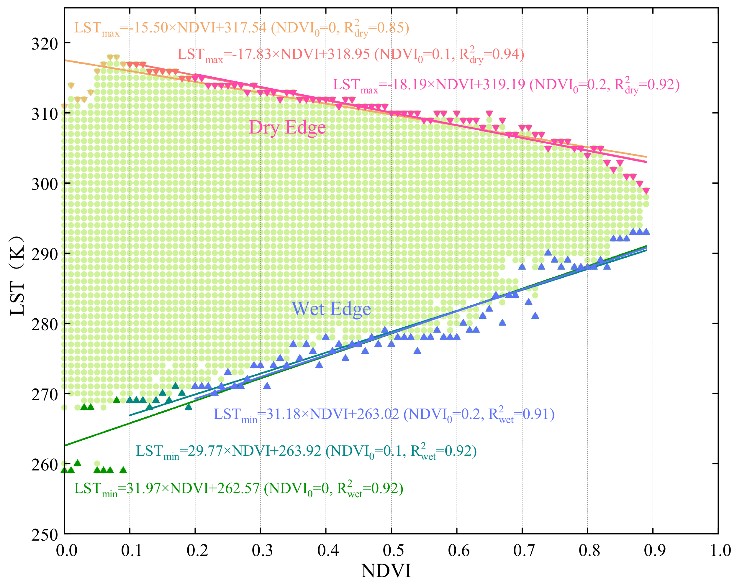
3.1.2. Interpretation of the NDVI-LST Triangle Space

Previous researchers have noted a negative relationship between NDVI and LST, which usually forms a triangular shape [29,65,66,67] in the scatter plot of NDVI against LST. It can be related to vegetation coverage and SM, thus is widely used to estimate SM [31,34,68,69,70,71,72].
The conceptual NDVI-LST triangle space is shown in Figure 2. In the triangle, the edges in red or blue can be defined as representing extreme conditions of SM and evapotranspiration. While the decreasing dry edges in red (CE, C’E’) represent limiting conditions (maximum LST and no evapotranspiration) of SM and evapotranspiration for different land cover classes, the horizontal wet edges in blue (DE, D’E’) represent the LST (LSTmin) under unlimited water access conditions and potential evapotranspiration. The pixels closest to the dry edge reflect extremely stressed surfaces with low SM. As green vegetation increases along the x-axis, LSTmax declines. Theoretically, in the triangular space, the temperatures of full vegetation cover and bare soil are the same when soil moisture is saturated [46]. The left and right edges (CD, C’D’) represent bare soil, ranging from dry to wet (LSTmax to LSTmin, respectively). Thus, the green color lines in the NDVI-LST space can be considered as a set of SM contours and the location of a pixel in the NDVI-LST triangular space is influenced mainly by SM availability (Figure 2).

3.1.3. Temperature Vegetation Dryness Index (TVDI)

To obtain information on RSM, the spatial distribution of TVDI shows clearly that TVDI is higher (maximum 1) and soil moisture is lower (water-stressed) at the dry edge, whereas TVDI is lower (minimum 0) and soil moisture is higher (saturated) at the wet edge [44]. The dryness index TVDI acquired from the NDVI-LST triangle space is defined by Sandholt et al. [29] as follows:
TVDI = LST LST min LST max LST min
where LST is the MODIS-derived LST in a given pixel, LSTmin refers to the minimum LST in the triangle space defining the wet edge at a given NDVI, LSTmax is the maximum LST in the triangle space defining the dry edge at a given NDVI.
As demonstrated in Figure 2, both dry and wet edges in the NDVI-LST triangle space are linearly regressed for an area large enough and the corresponding formula are shown as:
LST max = a dry   ×   NDVI + b dry
LST min = a wet   ×   NDVI + b wet
with Equations (5) to (6), Equation (4) for TVDI can be transformed as follows [8,10,75,76]:
TVDI = LST a wet   ×   NDVI + b wet a dry   ×   NDVI + b dry a wet   ×   NDVI + b wet
where a wet , a dry , b wet , and b dry are the linear fitting coefficients (slope and intercept) defining the dry and wet edges.

3.1.4. Applying Initial NDVI0 for Determination of TVDI

The scatterplot for the relationship between NDVI and LST, exemplified by DOY 113, is demonstrated in Figure 3. As the initial NDVI0 increases, both dry edge and wet edges change slightly. Such relationships (LSTmax or LSTmin and NDVI) are indicated when the initial NDVI0 equals 0, 0.1, and 0.2, respectively, with the linear equations in the scatterplot (Figure 3), positive slope values for the dry edge equations, and negative slope values for the wet edge equations. Thus, the TVDI value for a given pixel, to some extent, is influenced by the fluctuated wet or dry edge. Additionally, the TVDI-based model is more applicable to vegetated land with relatively high NDVI. In order to improve TVDI-based RSM retrieval, it is necessary to test NDVI0 from 0 to 0.5 with a small interval of 0.01 in the study area. The new TVDI value was calculated based on a given NDVI0 in an iteration. It is worth mentioning that the pixels of NDVI less than 0 were ignored in this study since these pixels are mainly water body, cloud, or snow,which are regarded as 100% RSM.

3.2. Establishment of the Retrieval Model

The linear relationship between ATI and in situ RSM measurements, and between TVDI and in situ RSM measurements is simple, but which subregion using the ATI-based model or TVDI-based model for the whole study area seems rather complex. In that case, it is challenging to get corresponding reliable thresholds for subregions using different models. We proposed an iteration procedure to obtain optimal NDVI thresholds for subregions. In detail, as can be seen in Figure 4, the initial NDVI (NDVI0) should be used first to determine the TVDI-based model. Once the NDVI0 is determined, the wet and dry edges and their linear regression equations (Equations (5) and (6)) will be formed with the specific value of adry, awet, bdry, bwet, R2wet, and R2dry. The second and third NDVI threshold (NDVIATI and NDVITVDI, respectively) are then used to divide the entire study area into three subregions, namely the ATI subregion (ATI), the TVDI subregion (TVDI), and the ATI/TVDI subregion (MATI/TVDI). While the area with NDVI less than NDVIATI was regarded as the ATI subregion, where only the ATI-based model was applied to the retrieval of RSM, the area with NDVI greater than NDVITVDI was regarded as the TVDI subregion where only the TVDI-based model was applied. For the ATI/TVDI subregion (NDVIATI ≤ NDVI ≤ NDVITVDI), the average of ATI and TVDI (MATI/TVDI) was used to estimate RSM. The procedure of calibration, that the linear regression between ATI and in situ RSM measurements, between MATI/TVDI and in situ RSM measurements, and between TVDI and in situ RSM measurements, was performed in each iteration for the three subregions.
Here, we took the ATI subregion as an example. Both NDVI0 and NDVIATI ranged from 0 to 0.5 with a small interval of 0.01 and NDVITVDI ranged from 0 to 0.7 with an interval of 0.01 in the iterative optimization procedure. For one iteration, linear regression analysis was performed to examine the relation between ATI and in situ RSM measurements through the 10-fold crossing-calibration in the calibration process. In the validation procedure, ten sets of statistics between in situ RSM measurements and estimated RSM, including R-values, RMSE (root mean square error), MAE (mean absolute error), and the p-values for significance tests were computed with corresponding NDVI0, NDVIATI, and NDVITVDI thresholds. The mathematical expressions of the goodness validation between in situ RSM measurements and estimated RSM in the study are presented in Table A2. Then the average R values of ten rounds were calculated as measures of the goodness-of-fit between in situ RSM measurements and estimated RSM. The calibration and validation steps in the ATI subregion were performed simultaneously in the TVDI subregion and the ATI/TVDI subregion with corresponding NDVI0, NDVIATI, and NDVITVDI thresholds.
After completing all iterations, the NDVI thresholds corresponding to maximum R-value were chosen as the optimal thresholds when NDVI0, NDVIATI, and NDVITVDI thresholds exist simultaneously for RSM estimation in the whole CLP. The subregional RSM was estimated by applying selected optimal thresholds (NDVI0, NDVIATI, and NDVITVDI) for each period. Generally, the whole region was divided into three subregions by selected NDVIATI and NDVITVDI, and the overall RSM map, ultimately produced using a combination of the subregional RSM for each period. The completely iterative optimization procedure was repeated for all 46 periods in 2017. The spatiotemporal distribution of RSM was characterized by derived RSM imagery.
In terms of establishing NDVI thresholds, it is worth mentioning that NDVI0 should be smaller than or equal to NDVIATI, which is smaller than or equal to NDVITVDI (NDVI0 ≤ NDVIATI ≤ NDVITVDI). In this way, the TVDI value for each pixel could be calculated in the TVDI subregion. Similarly, the mean of ATI and TVDI for each pixel could be assigned in the ATI/TVDI subregion.

3.2.1. RSM Estimation for the ATI Subregion

In the following experiment, the focus was on identifying an NDVIATI threshold which allows the CLP to be divided into two subregions first. The area with NDVI less than or equal to NDVIATI (hereinafter ATI subregion) was assigned ATI value. The NDVIATI threshold was selected from 0 to 0.5 with a small interval of 0.01. In general, ATI has a positive correlation with RSM, and the ATI-based model is mainly applied to barely or sparsely vegetate ground [77]. Thus, we chose the area where NDVI was less than the NDVIATI threshold as the ATI subregion for the application of the ATI-based model in the calibration process. The regression parameters ( a ATI   and b ATI ) of the ATI subregion can be calculated using the following empirical linear equation:
RSM = a ATI   ×   ATI + b ATI
where RSM is the relative soil moisture value (unit: %) measured at depth of 20 cm by automatic soil moisture observation stations, ATI is the ATI value for a given pixel (NDVI ≤ NDVIATI), a ATI and b ATI are the regression parameters using ATI value and in situ RSM measurements.

3.2.2. RSM Estimation for the TVDI Subregion

In this study, the TVDI-based model was also used for RSM estimation. Since ATI generally results in weaker correlations with in situ RSM measurements in vegetated areas than TVDI, it is better to consider the application of TVDI for RSM estimation to the TVDI subregion. To outline the TVDI subregion, an additional threshold of NDVITVDI was considered, which was greater than or equal to NDVIATI. The NDVITVDI threshold was selected from 0 to 0.7 with an interval of 0.01. The area for which NDVI was larger than or equal to NDVITVDI was regarded as the TVDI subregion and the TVDI value was applied to such an area for constructing a linear regression model with in situ RSM measurements in the calibration process. Therefore, the calibration of the model is presented as follows:
RSM = a TVDI   ×   TVDI + b TVDI
where TVDI refers to the TVDI for a given pixel (NDVI ≥ NDVITVDI) ;   a TVDI and b TVDI are the regression parameters using TVDI value and in situ RSM measurements

3.2.3. RSM Estimation for the ATI/TVDI Subregion

To achieve higher RSM estimation accuracy, both ATI and TVDI are utilized to retrieve the RSM of the remaining area of the CLP (i.e., the CLP except for the ATI subregion and TVDI subregion; hereinafter as the ATI/TVDI subregion), which overcomes the limitations of a single method (ATI-based or TVDI-based models). Zhao et al. (2012) proposed a model-level integrated approach to effectively retrieve large-scale daily soil moisture. They regarded the average value of soil moisture from the ATI-based model and the TVDI-based model as the soil moisture when NDVI ranged from 0.1 to 0.18 [78]. Wang et al. (2020) applied the soil moisture obtained by averaging the PDI (perpendicular drought index)-based model and TVDI-based model [10]. In our study, the average of ATI and TVDI value was calculated where NDVI varied from NDVIATI and NDVITVDI in the ATI/TVDI subregion, as a joint index MATI/TVDI ranging from 0 to 1. However, the nature of the correlation (positive or negative) between MATI/TVDI and in situ RSM measurements varied. The calibration equations for calculating MATI/TVDI and in situ RSM measurements in the ATI/TVDI subregion are given below:
M ATI / TVDI = ATI + TVDI 2
RSM = a ATI / TVDI   ×   M ATI / TVDI + b ATI / TVDI
where M ATI / TVDI   is the average of ATI and TVDI for a given pixel (NDVIATI < NDVI < NDVITVDI) and a ATI / TVDI and b ATI / TVDI are the regression parameters using M ATI / TVDI and in situ RSM measurements.

3.2.4. Calibration and Validation

The 10-fold cross-calibration method (traditionally called 10-fold cross-validation in statistics [79]) would be used to improve the accuracy of RSM estimation. In general, this method is used primarily for assessing how accurately a predictive model performs [80,81]. Moreover, to reduce the variability of the calibration, 10 rounds of 10-fold cross-calibration are performed between generated dryness indices (ATI, TVDI, MATI/TVDI) and in situ RSM measurements in those three subregions, respectively.
The ATI subregion was taken as an example to illustrate the calibration and validation procedures (Figure 5). The paired ATI and in situ RSM measurements were regarded as original samples and the RSM estimation was allowed only when the number of available RSM observation stations was greater than 20 in the ATI subregion. In detail, one round of cross-calibration involved random splitting of the original samples of paired ATI and in situ RSM measurements into complementary 10 subsamples with 9 as training data and one as testing data. The detailed calibration is shown in Figure 6. Training data in our analysis were calibrated using Equation (8) one-fold. The estimated RSM for one-fold was calculated using ATI value in testing data and obtained regression parameters (aATI and bATI) in the process of one-fold calibration. In this way, one group of estimated RSM and in situ RSM measurements was generated. We repeated this process until every 10-fold served as the testing data in practice. After the 10th fold was accomplished, we collected 10 groups of estimated RSM and in situ RSM measurements as the validation data. The validation results, including RATI, RMSE, and MAE, as well as the p-value for a significance test, were computed, which was just called “one-round”.
The original samples of paired ATI and in situ RSM measurements would be randomly split into 10 subsamples and the same calibration and validation were performed again. After ten rounds of iterations, we averaged the ten rounds of validation outcomes of the R ( R A T I ¯ ) as the reference to evaluate corresponding NDVI thresholds, since the ATI subregion was generated from NDVIATI. It should be noted that the same procedures of calibration and validation were conducted in the TVDI subregion as well as in the ATI/TVDI subregion. Similarly, the R T V D I ¯ value was determined by the thresholds NDVI0 and NDVITVDI. The three thresholds (NDVI0, NDVIATI, and NDVITVDI) together determined the value of R A T I / T V D I ¯ .

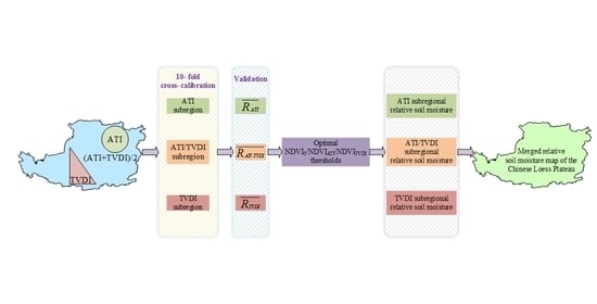
3.2.5. Identifying and Applying the Optimal NDVI Thresholds for Subregional RSM Retrieval

The optimal NDVI thresholds were identified dependent on the average validation results of the correlation coefficient ( R A T I ¯ , R A T I / T V D I ¯ and R T V D I ¯ ), which directly impact the accuracy of RSM retrieval. It is worth mentioning that the NDVI thresholds corresponding to maximum R-value among three subregions were chosen as the optimal thresholds when NDVI0, NDVIATI, and NDVITVDI thresholds exist simultaneously for one period. Here, we could not guarantee that all three subregions reach the highest averaged R-value in their subregions at the same time with selected optimal NDVI thresholds. To some extent, subregional RSM with the lower R-value could not be produced.
In addition, it was preferable to set NDVIATI larger than or equal to NDVI0 and NDVITVDI larger than or equal to NDVIATI, namely NDVI0 ≤ NDVIATI ≤ NDVITVDI. In that case, the TVDI value was given to all pixels in the TVDI subregion when NDVI0 was less than or equal to NDVITVDI. NDVIATI less than or equal to NDVITVDI could prevent certain overlapping between the ATI subregion and the TVDI subregion. If NDVI0 was bigger than NDVIATI, there would be some pixels filled with ATI value rather than the average of ATI and TVDI value in the ATI/TVDI subregion. As mentioned before, both NDVI0 and NDVIATI range from 0 to 0.5, and [0, 0.7] is for NDVITVDI with an interval of 0.01. The total number of NDVI thresholds collocation for one period is 48,620, which means a maximum of 48,620 iterations performed in three subregions when the number of available RSM observation stations was greater than 20.

3.2.6. Combining Subregional RSM Maps to Generate overall RSM Maps

The subregional RSM was separately estimated using the corresponding model with selected optimal NDVI thresholds. Then, we combined them to obtain an overall RSM map for one period. The combined equations were used as follows:
R S M overall = R S M A T I = a A T I   ×   A T I + b A T I                       N D V I 0 , N D V I A T I R S M A T I / T V D I = a A T I / T V D I   ×   A T I + T V D I 2 + b A T I / T V D I     N D V I N D V I A T I , N D V I T V D I R S M T V D I = a T V D I   ×   T V D I + b T V D I               N D V I N D V I T V D I ,1
where R S M o v e r a l l represents RSM obtained with the optimal NDVI thresholds using the combined method, R S M A T I   and R S M T V D I are the RSM estimated by the ATI-based and TVDI-based models, respectively, R S M A T I / T D V I represents the RSM estimated by the ATI/TVDI joint model, a A T I and b A T I are coefficients from fitting the ATI values and in situ RSM measurements in the ATI subregion, a T V D I and b T V D I are coefficients from fitting the TVDI values and in situ RSM measurements in the TVDI subregion, a A T I / T V D I and b A T I / T V D I are coefficients from fitting the average value of ATI and TVDI and in situ RSM measurements in the ATI/TVDI subregion, and   N D V I A T I and N D V I T V D I are the selected optimal thresholds for generating three subregions.
To illustrate the improvement in the proposed method, ATI-based and TVDI-based models were solely applied for RSM estimation. Quantitative comparison between observed and estimated RSM was performed at some stations (even distributed over the CLP) on DOYs 17 (in winter), 97 (spring), 137 (spring), 161 (summer), 209 (summer), 297 (autumn), 329 (autumn) and 353 (winter).

4. Results

4.1. Evaluation of the Calibration and Validation Results

4.1.1. Comparing Validation Results

While 46 periods of data were analyzed in 2017 (DOYs 1-361 with an 8-day interval), only 38 RSM maps (except for DOYs 1, 9, 33, 65, 73, 201, 225, and 241) were obtained eventually using the above-mentioned models over the study area. For the CLP, winter (December-February) was the coldest season of 2017 (Julian day/DOY337-361 and DOY 1-49). While DOY 57 to 145 and DOY 153 to 233 were generally considered as spring and summer, respectively, the rest of the days of the year belonged to autumn (DOY 241-329). It should be noted that 74-213 stations in the CLP were used and the number of stations (~100) used in winter was less than the other periods (usually exceeding 200) (Table 3). Fewer measurements were available for the study area due to RSM not being measured when the soil was frozen. The RSM maps on DOYs 1, 9, 33, 65, 73 were uncalculated in the cold days since the average R-value was relatively low (less than 0.18).
The last column of Table 3 has the highest R values in the validation corresponding to optimal NDVI thresholds—after 10 rounds of 10-fold cross-calibration for each 8-day data. As the DOY increased, the value of R fluctuated over time with no clear trends, while the R of DOY 313 imagery was the largest, up to 0.75 ± 0.008, using the ATI/TVDI joint model, and the minimum R was 0.17 ± 0.060, using the ATI/TVDI joint model, on DOY 273. In addition, the error of the model was calculated with the largest and smallest RMSE values being 6.79 ± 0.212% (DOY 273) and 2.83 ± 0.039% (DOY 313), both using the ATI/TVDI joint model. In terms of MAE, the maximal MAE was 0.50 ± 0.066 using the ATI/TVDI joint model on DOY 361 and the minimum MAE 0.01 ± 0.009 using the ATI-based model on DOY 161.

4.1.2. The NDVIATI and NDVITVDI Thresholds for Generating Subregions

As shown in Table 3, no fixed NDVIATI and NDVITVDI thresholds were applying to data throughout the year. In this study, it is observed that most of the identified NDVIATI thresholds were in the vicinity of 0.17 in the first four months and in November and December. However, NDVIATI in almost the entire summer (DOYs 153-217) was larger (more than 0.3) than in the other seasons. It is noted that only a few periods, e.g., DOYs 129, 161, and 257, saw their NDVIATI value approximated the upper limit (0.5) that was set. Table 3 also shows that the smallest NDVIATI (0.14) was used for DOY 25 and 49.
Regarding the NDVITVDI thresholds over the study area, the months from May to September witnessed larger NDVITVDI values (~0.5). Additionally, the minimum NDVITVDI appeared in the later months of 2017 when NDVIATI was quite small as well. As for modeling, the joint index MATI/TVDI was used for nearly all periods (36/38). In other words, most of the RSM was estimated using the ATI/TVDI joint model in the ATI/TVDI subregion. The value of R was relatively low (0.34 ± 0.044 on DOY 161 and 0.32 ± 0.018 on DOY 361, respectively) solely using the TVDI-based model, which is in agreement with the results from Lu et al. [17]. The subregional RSM maps were merged for DOY 257 and DOY 361 (Figure 7 and Figure 8). There are some discrepancies at the boundary of the subregions for the imagery of two periods because they are constructed according to different NDVI ranges—namely the selected optimal NDVI thresholds.

4.1.3. The Threshold NDVI0 for TVDI

Our results demonstrate that NDVI0 was generally small, particularly in the first four months and the last month of the year. It was 0, at its lowest, on DOYs 41, 217, 289, 313, and 337, rising to 0.43 on DOY 193. The NDVI and LST on the dry edge and wet edge generally showed significant correlations with R d r y 2 and R w e t 2 up to 0.97 on DOY 121 and 0.92 on DOYs 81 and 113, respectively (Table 3).
The parameters of dry and wet edge equations (slope a, intercept b, and correlation coefficient R) are illustrated in Figure 9 for a better understanding of the fitting results. These observations were consistent with the TVDI concept—i.e., the dry edge with a negative slope and the wet edge with a positive slope formed the NDVI-LST triangular space for all the periods of 2017 (Figure 9). Despite similar patterns, the slope of dry edge (adry) had higher values in cold days than on warm days, which was the opposite in the case of the slope of wet edge (awet). The intercepts bdry and bwet also had similar trends (values were higher on warm days than on cold days) but the trend of bdry was more prominent. Regarding the correlation coefficients,   R d r y 2 was generally higher than   R w e t 2 .

4.2. Analysis of RSM Estimation Using an Optimal Model and Optimal NDVI Thresholds

4.2.1. Calibration and Validation Analysis of RSM Estimation

The subregional RSM was estimated by applying the optimal thresholds (NDVI0, NDVIATI, and NDVITVDI) for each period. In practice, no RSM estimation was performed for subregions with low R-values. According to Table A3, in the process of calibration, the linear regression between three indices (ATI, MATI/TVDI, and TVDI) and in situ RSM measurements was various with both positive and negative relationships in the certain subregion.
For example, MATI/TVDI showed a positive correlation with in situ RSM measurements on most of the periods (~80%) except for DOY 137, 145, 161, 249, 257, 273, 281, and 289. In our research, two negative slope values occurred in the fitting equation between ATI and in situ RSM measurements on DOY 25 and 153. TVDI was positively correlated with in situ RSM measurements on DOYs 161 and 361 with the regression coefficient 0.24 and 0.14, respectively, in the calibration procedure. The largest R2 was 0.66 and 1 in the calibration and validation process, respectively. It is worth mentioning that the fitting outcomes for each period passed the hypothesis test with confidence of 0.1 (Table A3).

4.2.2. Estimated RSM Maps over the CLP

The spatial distribution of RSM is illustrated by season (Figure 10, Figure 11, Figure 12 and Figure 13). It is clear that only the RSM in the pixels whose NDVI was within the specified NDVI range could be estimated for each imagery. The used subregions could be marked in the upper left corner of each subfigure. While NDVIATI < NDVI < NDVITVDI means that the joint index MATI/TVDI was used for the ATI/TVDI subregion, NDVI ≤ NDVIATI, and NDVITVDI ≥ NDVI represent that indices ATI and TVDI were used for the ATI subregion and TVDI subregion, respectively.
The estimated RSM tended to cluster in the northwestern of the study area when the ATI-based model was applied (Figure 10b,c, Figure 12a and Figure 13a,b,d). These regions are mainly covered by sparse vegetation or bare soil because of lower NDVI. However, the TVDI-based model could estimate RSM over the southern and eastern parts (Figure 10h).
From the perspective of RSM seasonal variation, RSM in red color was low, particularly in the southern part (RSM less than 5%) (Figure 10b,d–h) and RSM in green color was relatively high in northern China in winter (Figure 10a,e,f,h). The overall RSM in green and light blue color gradually increased with a rise to 40% in the west area in spring (Figure 11d and Figure 10e,f,g). Nearly 50% of the RSM in ultra-blue color was observed in the west area in summer (Figure 12c and Figure 10d–h). RSM with the yellow and light green color in most areas increased to its peak in August and September (Figure 12h,i and Figure 13a–d). Then RSM in orange and red color dropped gradually in the following days (Figure 13g,i–k).

5. Discussion

5.1. Applicability of the ATI/TVDI Joint Model

In this paper, the indices ATI and TVDI were used for modeling and estimating RSM in the CLP during the whole year of 2017. NDVI is a vital factor influencing not only the wet and dry edges for obtaining TVDI but also the application of models in the subregions. Compared to the ATI-based and TVDI-based models, the ATI/TVDI joint model achieved higher accuracy in calibration and the ATI-based and TVDI-based models’ advantages had a good performance in RSM estimation. It is observed from Table A3 that both ATI-based and TVDI–based models are seldom used for RSM estimation, which was consistent with the observations reported by Lu [17]. Du et al. performed the original TVDI and the modified TVDIm for drought monitoring in semi-arid regions of China and found that the improved TVDIm exhibits better performance in both meteorological and agricultural drought monitoring compared to the original TVDI. The R2 between TVDIm and in situ RSM was 0.21, which is lower than most of the R2 in calibration (Table A3) [73]. Zhang et al. calculated the correlation coefficients between TVDI and SM at depths of 10 cm and 20 cm in Southwest China and the maximum R2 was 0.29 on DOY 281, which is lower than our maximum R2 (0.66) on DOY 137 and 0.46 on DOY 281 [47]. NDVI0 that we applied played an important role in RSM estimation by the TVDI-based model according to the selected optimal NDVI thresholds. Comparative analysis indicated that the ATI/TVDI joint model had higher applicability (accounting for 36/38 periods) than the ATI-based and TVDI-based models. As shown in Table A3, there is no significant regularity for the parameters in the fitting equations since the studied period is short.
Figure 14 and Table A4 demonstrate that the combined model we applied for RSM retrieval shows the improvements solely over ATI- and TVDI-based models with the minimum difference between the estimated RSM and the observed RSM and maximum R-value (correlation coefficient) in calibration. The comparative analysis indicated that the RSM estimated by the TVDI-based model was closest to the actual RSM measured on-site compared to the ATI-based model, which shows a good agreement with Hsu’s research results [18]. Jiao et al. investigated the relationships between SM and vegetation coverage and suggested that excessive reliance on afforestation was risky for the improvement of vegetation coverage in arid and semi-arid regions and we, thus, need to focus on the soil moisture conditions during large-scale re-vegetation. Thus, the methodology presented in this study has clearly improved the estimation of SM throughout the year of 2017 over the CLP compared to other methods. It highlights the importance of vegetation coverage in soil moisture estimation and the possibility of producing a potentially complete SM estimation map for such a large area by merging subregional maps. Some researchers just performed SM estimation on a small scale at a specific period using the TVDI-based model [38,47,71]. To further this work, more research is required to examine the correlation between other indices and climate regimes as well as using a longer time series MODIS and in situ RSM measurements when they become available [36,82]. It should be noted that there were no in situ RSM measurements in the Ningxia province (Figure 1) and this blank area should be filled when station measurements become available in the future.
In the process of calibration, the 10-fold cross-calibration method was rarely applied to linear regression analysis between satellite-based indices and in situ RSM measurements, and this method indeed improved the accuracy of RSM estimation in terms of validation outcomes with limited in situ measurements. In short, the procedure from identifying NDVI thresholds to modeling could be widely applied because it enables determining an optimal model for RSM estimation.

5.2. Estimation of RSM in the CLP

To show the effectiveness of the selected optimal NDVI thresholds, RSM maps at an 8-day interval were produced for the entire CLP. The limited number of in situ RSM observation stations in the frozen period led to difficulties in ensuring better model calibrations. Regions with the frozen ground or snow-covered are generally masked out [83]. Hence, the average correlation coefficient (R) for verification was generally low at that time. In general, the soil thawing–freezing process occurs from November to March in this area. RSM rises dramatically during the thawing period and decreases rapidly in the freezing period and this phenomenon was not evident in our results. Liu et al. claimed that the TVDI-based method is suitable for obtaining satisfactory outcomes if the effects of both altitude and frozen soil are considered [34]. The main reason for the sudden rise in RSM in the autumn and summer images was very likely to be regional increases in precipitation in the rainy season [84,85,86,87]—e.g., in the west area (Qinghai province) from DOY 241 to 249 and in the northwest area from DOY 265 to 273.
In terms of incomplete RSM maps, we have here some explanations that the overall map was generated by a combination of subregional RSM for one period and it failed to select the highest R-value in certain subregions resulting in no subregional RSM map produced. The reason for that might be the limited availability in situ RSM measurements in those subregions.

5.3. Innovations and Limitations

Studies on RSM estimations and spatiotemporal dynamics on regional or continental scales using MODIS data are important for understanding the overall pattern and developing retrieval model [88]. In our study, an iteration procedure that allows us to identify optimal NDVI thresholds and models for estimating RSM with 10 rounds of 10-fold cross-calibration and validation. We separately used three models (the ATI-based model, the TVDI-based model, and the ATI/TVDI joint model) based on optimal NDVI thresholds in the corresponding subregions for retrieving the 8-day RSM from MODIS imagery with in situ RSM measurements. The combination of different subregional RSM maps for the overall map at large scales, as demonstrated in our case study, provides a new perspective for accuracy RSM estimation.
However, we here would like to highlight some of the weaknesses in this study that can be improved in future work. The MODIS images and in situ RSM measurements from observation stations did not spatially match very well and comparing the RSM estimated from 8-day composite MODIS data with the in situ RSM measurements might decrease the modeling accuracy. In addition, some environmental factors, such as soil type, latitude, topography, and hydrology, can affect the accuracy of RSM estimation and should be considered to improve the retrieval model.

6. Conclusions

In this study, we proposed an iteration procedure that allows us to identify optimal NDVI thresholds by performing 10 rounds of 10-fold cross-calibration and thus to estimate the region-specific relative soil moisture of the Chinese Loess Plateau in 2017 using different models—namely the ATI-based model, the TVDI-based model, and the ATI/TVDI joint model. The key findings and main conclusions are as follows:
  • The whole study area was divided into three subregions by selected optimal NDVI thresholds and the overall RSM map was produced by combining subregional RSM maps over the CLP. This combination-based approach provides a new perspective for the mapping of RSM over large geographical areas.
  • Spatiotemporal and comparative analysis indicated that the ATI/TVDI joint model had higher applicability (accounting for 36/38 periods) and accuracy than the ATI-based and TVDI-based models. The ATI-based model is only suitable for bare soil and sparsely vegetated areas while the TVDI-based model is more applicable to moderately or highly vegetated areas.
  • The 10-fold cross-calibration method in the iteration procedure improves overall reliability and effectiveness in terms of identifying optimal NDVI thresholds.
Our study has innovated the mapping of RSM by applying different estimation models to different land covers; however, it remains necessary to validate the ATI/TVDI joint method with more measurements from various environments. The findings of this study will contribute to decision-makers in agricultural management and formulating policies of the Chinese Loess Plateau.

Author Contributions

Conceptualization, L.Y. and L.L.; methodology, L.Y.; software, S.H.; validation, L.Y.; resources, T.Z., J.Z. and L.C. (Liang Cheng); writing—original draft preparation, L.Y. and T.Z.; writing—review and editing, L.L. and L.C. (Longqian Chen); visualization, S.H., and W.L.; supervision, L.C. (Longqian Chen) and L.L. All authors have read and agreed to the published version of the manuscript.

Funding

This research was supported by the Fundamental Research Funds for the Central Universities (Grant No.: 2018ZDPY07).

Acknowledgments

The authors thank the China Meteorological Data Service Center (CMDC, http://data.cma.cn/) for providing all in situ RSM data. The remote sensing data were freely provided by the NASA Land Processes Distributed Active Archive Center (LP DAAC, https://lpdaac.usgs.gov/). Furthermore, we appreciate the editors and reviewers for their constructive comments and suggestions.

Conflicts of Interest

The authors declare no conflict of interest.

Abbreviations

The following abbreviations are used in this manuscript:
ATI Apparent thermal inertia
CLP Chinese Loess Plateau
CMDC China Meteorological Data Service Center
DOY The day of the year
LST Land surface temperature
MATI/TVDI Mean of the value of ATI and TVDI
MAE Mean absolute error
MODIS Moderate Resolution Imaging Spectrometers
MRT MODIS Reprojection Tool
NDVI Normalized Difference Vegetation Index
NDVI0Initial NDVI for TVDI
NDVIATINDVI threshold for ATI subregion
NDVIATI/TVDNDVI threshold for ATI/TVDI subregion
NDVITVDINDVI threshold for TVDI subregion
PDIPerpendicular drought index
R2Coefficient of determination
RCorrelation coefficient
RMSE Root Mean Square Error
RSM Relative soil moisture
SMSoil moisture
TVDI Temperature Vegetation Dryness Index
UTC The Coordinated Universal Time

Appendix A

Table A1. Locations of the automatic RSM observation stations within the Chinese Loess Plateau.
Serial NumberStationLatitude
(°E)
Longitude
(°N)
Serial NumberStationLatitude
(°E)
Longitude
(°N)
152,76537.38101.614453,48840.04113.59
252,79737.19104.064553,49040.44114.06
352,85536.69101.254653,51239.79106.80
452,86236.97101.664753,51340.72107.37
552,86336.82101.954853,52240.05107.84
652,86636.73101.754953,52939.09107.96
752,86836.02101.375053,53339.81108.71
852,86936.49101.585153,54339.82110.01
952,87436.49102.415253,54539.56109.71
1052,87536.5102.105353,54739.10109.03
1152,87636.33102.845453,55339.85111.22
1252,87736.10102.265553,56239.92111.66
1352,88436.35103.935653,56439.37111.21
1452,88536.75103.255753,56539.44111.50
1552,89536.57104.695853,57439.52112.27
1652,89636.55104.155953,57639.51112.82
1752,96335.94102.026053,57839.37112.43
1852,97235.85102.466153,57939.05112.92
1952,97435.54102.036253,58039.83113.10
2052,98035.97103.306353,58239.71113.67
2152,98235.48103.566453,58439.56113.16
2252,98335.87104.146553,58539.17113.26
2352,98435.58103.186653,59039.74114.26
2452,98535.41103.346753,59439.44114.22
2552,98635.36103.866853,64438.59108.83
2652,99335.68105.066953,64638.27109.78
2752,99535.58104.607053,65138.83110.46
2852,99835.13104.207153,65937.97111.01
2953,33741.05108.287253,66238.71111.57
3053,34841.02109.137353,66338.93111.82
3153,41940.33106.997453,66538.28111.63
3253,42040.87107.137553,66638.36111.94
3353,43340.73108.657653,66938.07111.81
3453,44640.53109.887753,67338.74112.71
3553,45540.55110.557853,67438.39112.69
3653,45740.39110.037953,67638.5112.98
3753,46340.86111.578053,67737.94112.48
3853,46440.73111.178153,67838.07112.65
3953,46640.76111.718253,67937.75112.54
4053,46740.25111.258353,68138.84113.36
4153,46940.4111.828453,68538.08113.42
4253,47839.99112.468553,68737.79113.63
4353,48640.37113.778653,72537.6107.60
8753,73038.19107.4713053,88236.06113.03
8853,73237.86108.7213153,88436.51113.03
8953,73537.6108.8013253,88836.20113.44
9053,73836.92108.1813353,90635.52105.71
9153,74037.96109.2913453,90835.21105.23
9253,74837.15109.6913553,91535.53106.66
9353,75437.49110.2613653,91735.22106.06
9453,75936.99110.8313753,92335.73107.63
9553,76337.90112.1713853,92435.07107.62
9653,76437.51111.1113953,92535.68107.19
9753,76737.33111.1814053,92635.34107.35
9853,76837.15111.7514153,92735.20106.62
9953,76937.24111.7814253,92835.30107.02
10053,77037.36112.3514353,92935.21107.77
10153,77137.41112.0514453,93036.45107.99
10253,77437.58112.3714553,93136.00109.38
10353,77537.42112.5914653,93435.78107.98
10453,77637.70112.7914753,93735.53107.89
10553,77737.51112.1414853,93835.17108.28
10653,77837.17112.1814953,94135.19109.58
10753,78037.91113.1515053,94235.79109.36
10853,78337.60113.7215153,94735.06109.08
10953,78837.33113.5715253,94834.89109.63
11053,82136.57107.3015353,95035.23110.15
11153,84536.60109.5015453,95435.62110.97
11253,85336.70110.9515553,95535.52110.46
11353,85636.46110.7515653,95635.42110.84
11453,85736.06110.1815753,95735.61110.71
11553,85936.09110.6615853,95835.17110.78
11653,86135.89111.3915953,95935.11111.07
11753,86337.06111.9416053,96135.65111.49
11853,86536.66111.5616153,96235.73111.70
11953,86636.23111.6616253,96335.65111.36
12053,86836.06111.4916353,96435.62111.21
12153,86936.58111.7016453,96535.50111.57
12253,87136.86112.8716553,96635.98111.83
12353,87236.76112.6916653,96735.33111.20
12453,87336.10112.8716753,96835.28111.66
12553,87436.25111.9016853,97035.69112.19
12653,87736.16112.2516953,97335.78112.94
12753,87836.51113.3617053,97535.49112.41
12853,87936.32112.8917153,97635.50112.86
12953,88036.34113.2317253,97835.09112.63
17356,09234.99104.6519457,04234.78109.19
17457,00134.75105.3319557,04334.80109.97
17557,00334.89106.8419657,04434.40109.23
17657,00434.73104.8819757,04534.40109.49
17757,01434.56105.8719857,04734.16109.32
17857,02034.36107.3919957,04834.40108.72
17957,02234.68107.8020057,05134.79111.19
18057,02434.44107.6520157,05234.88110.45
18157,02534.51107.3820257,05334.70110.71
18257,02634.37107.8820357,05534.59110.13
18357,02734.30107.7320457,06035.16111.22
18457,02934.49108.4520557,06134.84111.20
18557,03034.69108.1420657,06634.40111.67
18657,03134.83108.5520757,07134.80112.47
18757,03234.14108.2120857,07434.42112.40
18857,03334.56108.5320957,07634.74112.79
18957,03434.31108.2421057,08034.74112.97
19057,03534.54108.2521157,12334.29108.07
19157,03734.92108.9821257,13134.45108.97
19257,03834.28108.4821357,13234.14108.58
19357,04134.63108.93
Table A2. Mathematical expressions of the goodness of validation.
AbbreviationFormula
R2 i = 0 n O i O i ¯ P i P i ¯ i = 1 n O i O i ¯ 2 i = 1 n P i P i ¯ 2 2
R i = 0 n O i O i ¯ P i P i ¯ i = 1 n O i O i ¯ 2 i = 1 n P i P i ¯ 2
RMSE 1 n i = 1 n O i P i 2
MAE 1 n i = 1 n O i P i
STD i = 1 n P i P i ¯ 2 n
where O i and P i are the in situ RSM measurements and estimated RSM, O ¯ is the mean of in situ RSM measurements and P ¯ is the mean of estimated RSM.
Table A3. Data description and accuracy of these models for RSM retrieval.
DOYCalibrationValidation
ModelFitting EquationR2R2RMSEMAE
17ATI/TVDIy = 70.61x − 6.390.36 ***1.000.910.90
25ATIy = −239.74x + 19.980.28 *1.001.891.36
41ATIy = 259.54x + 2.7320.23 **1.000.990.74
49ATI/TVDIy = 32.06x + 1.640.20 **0.573.503.39
57ATI/TVDIy = 56.46x − 2.160.19 **0.971.000.97
81ATI/TVDIy = 35.11x + 6.410.38 **1.001.951.82
89ATI/TVDIy = 30.24x + 7.220.12 **0.432.962.49
97ATI/TVDIy = 20.34x + 8.260.30 ***0.483.573.56
105ATI/TVDIy = 36.52x + 8.200.10 **0.681.371.18
113ATI/TVDIy = 75.22x + 3.210.33 **0.672.111.38
121ATI/TVDIy = 71.01x − 0.7850.25 **0.552.091.93
129ATI/TVDIy = 49.47x − 2.460.43 **1.003.102.44
137ATI/TVDIy = −75.55x + 22.470.66 ***0.723.632.71
145ATI/TVDIy = −92.69x + 27.000.30 **0.932.812.48
153ATIy = −303.76x + 25.470.12 ***0.862.212.08
ATI/TVDIy = 70.05x + 2.730.22 **1.001.541.30
TVDIy = −26.78x + 21.120.24 **0.481.571.21
161ATI/TVDIy = −237.90x + 24.390.28 ***0.734.824.06
ATIy = 37.57x + 3.660.19 *0.925.253.82
169ATI/TVDIy = 53.34x + 5.720.44 **1.000.300.27
177ATI/TVDIy = 57.34x + 1.220.29 **0.482.121.60
185ATI/TVDIy = 67.79x − 1.690.42 ***0.993.472.88
193ATI/TVDIy = 38.35x + 1.110.11 *0.335.784.75
209ATI/TVDIy = 92.55x − 8.240.40 ***0.992.481.95
217ATI/TVDIy = 88.95x − 1.720.37 ***0.633.783.75
233ATI/TVDIy = 40.50x + 4.530.17 *0.603.392.61
249ATI/TVDIy = −235.66x + 27.890.32 ***0.392.772.36
ATIy = 54.38x + 5.530.23 **0.971.891.56
257ATI/TVDIy = −159.38x + 24.870.15 ***0.464.443.61
ATIy = 64.42x + 1.020.39 ***0.407.496.40
265ATI/TVDIy = 58.62x + 5.450.42 ***0.582.972.73
273ATI/TVDIy = −38.13x + 22.980.23 ***0.902.582.37
ATIy = 63.82x + 2.860.27 **0.286.755.73
281ATI/TVDIy = −57.46x + 32.930.46 ***0.661.851.81
289ATI/TVDIy = −35.11x + 25.120.15 **0.783.853.47
297ATI/TVDIy = 85.81x-8.400.47 ***0.980.890.81
305ATI/TVDIy = 53.85x + 4.760.23 ***0.702.792.40
313ATI/TVDIy = 21.85x + 7.780.15 *0.842.682.19
321ATI/TVDIy = 55.92x − 1.920.26 ***0.971.121.03
329ATI/TVDIy = 70.01x − 7.010.48 ***1.001.881.31
337ATI/TVDIy = 57.54x − 4.170.47 ***0.861.941.55
345ATI/TVDIy = 56.01x − 5.730.32 ***0.562.361.87
353ATI/TVDIy = 49.16x − 4.130.43 ***0.902.052.04
ATI/TVDIy = 62.46x − 5.290.41 ***0.811.891.80
361TVDIy = 22.66x − 1.250.14 ***0.532.912.43
ATI/TVDIy = 91.96x − 14.320.36 ***0.952.412.02
*, **, *** significant at p < 0.1, p < 0.05 and p < 0.01, respectively.
Table A4. Comparison of the estimated RSM and R-value in calibration using different models at some stations on DOYs 17, 353 (in winter), 97, 137 (spring), 161, 209 (summer), 297, and 329 (autumn).
Month/SeasonDOYStationObserved
RSM (%)
Combined ModelATI-Based ModelTVDI-Based Model
Estimated RSM (%)R-Value in CalibrationEstimated RSM (%)R-Value in CalibrationEstimated RSM (%)R-Value in Calibration
Jan/Winter1753,7350.805.990.609.510.376.960.45
53,9315.856.8910.997.90
57,05513.4312.3610.3211.49
53,97816.1511.1610.7610.77
53,9343.163.6011.205.71
Apr/Spring9753,5437.2210.580.5515.030.1214.540.11
53,65112.8214.6514.6615.15
53,68118.0817.4514.2915.79
53,75412.1812.1814.7515.22
53,95910.6812.0015.1015.20
May/Spring13753,4335.906.770.8110.830.0910.620.08
53,4697.507.0010.9310.63
53,7325.624.0111.2210.33
53,8638.218.1111.1810.70
53,6788.296.8511.1710.59
Jun/Summer16153,91511.7213.110.49/0.53/0.4414.170.4314.100.33
53,5858.7411.3613.1711.75
53,65910.3511.7213.6712.93
52,76529.3815.4215.027.30
57,08018.2317.7815.8814.91
Jul/Summer20953,4333.676.190.6314.510.0912.400.25
52,76533.9523.6213.8517.46
53,75416.2116.2314.9214.84
57,13113.5013.7514.3714.51
57,07113.0713.6914.2214.58
Oct/Autumn29753,74811.7712.980.6917.200.2816.640.27
57,05214.2014.1118.0317.21
53,87221.5820.9513.8318.73
53,67611.7812.2516.7216.28
53,77613.8215.2116.5317.28
Nov/Autumn32953,5124.007.220.6912.590.328.100.59
53,5533.535.7011.576.00
53,5852.996.5212.447.37
53,7809.1410.6612.1810.83
53,86816.5015.2611.9514.71
Dec/Winter35353,4782.720.990.66/0.648.820.300.590.49
53,5852.096.359.527.99
53,6513.407.479.098.67
57,05314.3013.299.6912.15
57,07116.9414.419.8313.13

References

  1. Seneviratne, S.I.; Corti, T.; Davin, E.L.; Hirschi, M.; Jaeger, E.B.; Lehner, I.; Orlowsky, B.; Teuling, A.J. Investigating soil moisture-climate interactions in a changing climate: A review. Earth Sci. Rev. 2010, 99, 125–161. [Google Scholar] [CrossRef]
  2. Njoku, E.G.; Kong, J.-A. Theory for passive microwave remote sensing of near-surface soil moisture. J. Geophys. Res. Space Phys. 1977, 82, 3108–3118. [Google Scholar] [CrossRef]
  3. Colliander, A.; Chan, S.; Kim, S.-B.; Das, N.; Yueh, S.; Cosh, M.H.; Bindlish, R.; Jackson, T.; Njoku, E. Long term analysis of PALS soil moisture campaign measurements for global soil moisture algorithm development. Remote Sens. Environ. 2012, 121, 309–322. [Google Scholar] [CrossRef]
  4. Ines, A.V.; Das, N.N.; Hansen, J.W.; Njoku, E.G. Assimilation of remotely sensed soil moisture and vegetation with a crop simulation model for maize yield prediction. Remote Sens. Environ. 2013, 138, 149–164. [Google Scholar] [CrossRef] [Green Version]
  5. Rahimzadeh-Bajgiran, P.; Berg, A.A.; Champagne, C.; Omasa, K. Estimation of soil moisture using optical/thermal infrared remote sensing in the Canadian Prairies. ISPRS J. Photogramm. Remote Sens. 2013, 83, 94–103. [Google Scholar] [CrossRef]
  6. Zhang, D.; Zhou, G. Estimation of Soil Moisture from Optical and Thermal Remote Sensing: A Review. Sensors 2016, 16, 1308. [Google Scholar] [CrossRef] [Green Version]
  7. Carlson, T.N.; Petropoulos, G.P. A new method for estimating of evapotranspiration and surface soil moisture from optical and thermal infrared measurements: The simplified triangle. Int. J. Remote Sens. 2019, 40, 7716–7729. [Google Scholar] [CrossRef]
  8. Holidi, H.; Armanto, M.E.; Damiri, N.; Putranto, D.D.A. Characteristics of Selected Peatland uses and Soil Moisture Based on TVDI. J. Ecol. Eng. 2019, 20, 194–200. [Google Scholar] [CrossRef]
  9. Rahimzadeh-Bajgiran, P.; Omasa, K.; Shimizu, Y. Comparative evaluation of the Vegetation Dryness Index (VDI), the Temperature Vegetation Dryness Index (TVDI) and the improved TVDI (iTVDI) for water stress detection in semi-arid regions of Iran. ISPRS J. Photogramm. Remote Sens. 2012, 68, 1–12. [Google Scholar] [CrossRef]
  10. Wang, H.; He, N.; Zhao, R.; Ma, X. Soil water content monitoring using joint application of PDI and TVDI drought indices. Remote Sens. Lett. 2020, 11, 455–464. [Google Scholar] [CrossRef]
  11. Price, J.C. Thermal inertia mapping: A new view of the Earth. J. Geophys. Res. Space Phys. 1977, 82, 2582–2590. [Google Scholar] [CrossRef]
  12. Wang, Y.; Bian, Z.; Lei, S.; Zhang, Y. Investigating spatial and temporal variations of soil moisture content in an arid mining area using an improved thermal inertia model. J. Arid. Land 2017, 9, 712–726. [Google Scholar] [CrossRef]
  13. Minacapilli, M.; Cammalleri, C.; Ciraolo, G.; D’Asaro, F.; Iovino, M.; Maltese, A. Thermal Inertia Modeling for Soil Surface Water Content Estimation: A Laboratory Experiment. Soil Sci. Soc. Am. J. 2012, 76, 92–100. [Google Scholar] [CrossRef]
  14. Wang, L.; Qu, J.J. Satellite remote sensing applications for surface soil moisture monitoring: A review. Front. Earth Sci. China 2009, 3, 237–247. [Google Scholar] [CrossRef]
  15. Lu, S.; Ju, Z.; Ren, T.; Horton, R. A general approach to estimate soil water content from thermal inertia. Agric. For. Meteorol. 2009, 149, 1693–1698. [Google Scholar] [CrossRef]
  16. Verstraeten, W.W.; Veroustraete, F.; Van Der Sande, C.J.; Grootaers, I.; Feyen, J. Soil moisture retrieval using thermal inertia, determined with visible and thermal spaceborne data, validated for European forests. Remote Sens. Environ. 2006, 101, 299–314. [Google Scholar] [CrossRef]
  17. Lu, X.J.; Zhou, B.; Yan, H.B.; Luo, L.; Huang, Y.H.; Wu, C.L. Remote Sensing Retrieval of Soil Moisture in Guangxi Based on Ati and Tvdi Models. ISPRS—Int. Arch. Photogramm. Remote Sens. Spat. Inf. Sci. 2020, 42, 895–902. [Google Scholar] [CrossRef] [Green Version]
  18. Hsu, W.-L.; Chang, K.-T. Cross-estimation of Soil Moisture Using Thermal Infrared Images with Different Resolutions. Sensors Mater. 2019, 31, 387. [Google Scholar] [CrossRef]
  19. Kang, J.; Jin, R.; Li, X.; Ma, C.; Qin, J.; Zhang, Y. High spatio-temporal resolution mapping of soil moisture by integrating wireless sensor network observations and MODIS apparent thermal inertia in the Babao River Basin, China. Remote Sens. Environ. 2017, 191, 232–245. [Google Scholar] [CrossRef] [Green Version]
  20. Fan, L.; Al-Yaari, A.; Frappart, F.; Swenson, J.J.; Xiao, Q.; Wen, J.; Jin, R.; Kang, J.; Li, X.; Fernandez-Moran, R.; et al. Mapping Soil Moisture at a High Resolution over Mountainous Regions by Integrating In Situ Measurements, Topography Data, and MODIS Land Surface Temperatures. Remote Sens. 2019, 11, 656. [Google Scholar] [CrossRef] [Green Version]
  21. Lei, S.-G.; Bian, Z.-F.; Daniels, J.L.; Liu, D.-L. Improved spatial resolution in soil moisture retrieval at arid mining area using apparent thermal inertia. Trans. Nonferrous Met. Soc. China 2014, 24, 1866–1873. [Google Scholar] [CrossRef]
  22. Taktikou, E.; Papaioannou, G.; Bourazanis, G.; Kerkides, P. Soil moisture assessment from MODIS data. Desalin. Water Treat. 2017, 99, 59–71. [Google Scholar] [CrossRef]
  23. Yu, Y.; Wang, J.; Cheng, F.; Chen, Y. Soil Moisture by Remote Sensing Retrieval in the Tropic of Cancer of Yunnan Province. Pol. J. Environ. Stud. 2020, 29, 1981–1993. [Google Scholar] [CrossRef]
  24. Markovic, S.B.; Stevens, T.; Mason, J.A.; Vandenberghe, J.; Yang, S.; Veres, D.; Újvári, G.; Timar-Gabor, A.; Zeeden, C.; Guo, Z.; et al. Loess correlations—Between myth and reality. Palaeogeogr. Palaeoclim. Palaeoecol. 2018, 509, 4–23. [Google Scholar] [CrossRef]
  25. Veroustraete, F.; Li, Q.; Verstraeten, W.W.; Chen, X.; Bao, A.; Dong, Q.; Liu, T.; Willems, P. Soil moisture content retrieval based on apparent thermal inertia for Xinjiang province in China. Int. J. Remote Sens. 2011, 33, 3870–3885. [Google Scholar] [CrossRef]
  26. Scheidt, S.; Ramsey, M.; Lancaster, N. Determining soil moisture and sediment availability at White Sands Dune Field, New Mexico, from apparent thermal inertia data. J. Geophys. Res. Space Phys. 2010, 115, 115. [Google Scholar] [CrossRef]
  27. Van Doninck, J.; Peters, J.; De Baets, B.; De Clercq, E.M.; Ducheyne, E.; Verhoest, N.E.C. The potential of multitemporal Aqua and Terra MODIS apparent thermal inertia as a soil moisture indicator. Int. J. Appl. Earth Obs. Geoinf. 2011, 13, 934–941. [Google Scholar] [CrossRef]
  28. Moran, M.; Clarke, T.; Inoue, Y.; Vidal, A. Estimating crop water deficit using the relation between surface-air temperature and spectral vegetation index. Remote Sens. Environ. 1994, 49, 246–263. [Google Scholar] [CrossRef]
  29. Sandholt, I.; Rasmussen, K.; Andersen, J. A simple interpretation of the surface temperature/vegetation index space for assessment of surface moisture status. Remote Sens. Environ. 2002, 79, 213–224. [Google Scholar] [CrossRef]
  30. Amani, M.; Salehi, B.; Mahdavi, S.; Masjedi, A.; Dehnavi, S. Temperature-Vegetation-soil Moisture Dryness Index (TVMDI). Remote Sens. Environ. 2017, 197, 1–14. [Google Scholar] [CrossRef]
  31. Holzman, M.E.; Rivas, R.E.; Bayala, M. Subsurface Soil Moisture Estimation by VI–LST Method. IEEE Geosci. Remote Sens. Lett. 2014, 11, 1951–1955. [Google Scholar] [CrossRef]
  32. Son, N.-T.; Chen, C.-F.; Chen, C.-R.; Masferrer, M.-G.-M.; Recinos, L.-E.-M.; Castellón, A. Multitemporal Landsat-MODIS fusion for cropland drought monitoring in El Salvador. Geocarto Int. 2018, 34, 1363–1383. [Google Scholar] [CrossRef]
  33. Moon, H.; Choi, M. Dryness Indices Based on Remotely Sensed Vegetation and Land Surface Temperature for Evaluating the Soil Moisture Status in Cropland-Forest-Dominant Watersheds. Terr. Atmos. Ocean. Sci. 2015, 26, 599. [Google Scholar] [CrossRef] [Green Version]
  34. Liu, Z.; Yao, Z.; Wang, R. Evaluating the surface temperature and vegetation index (Ts/VI) method for estimating surface soil moisture in heterogeneous regions. Hydrol. Res. 2017, 49, 689–699. [Google Scholar] [CrossRef]
  35. Shi, S.; Yao, F.; Zhang, J.; Yang, S. Evaluation of Temperature Vegetation Dryness Index on Drought Monitoring Over Eurasia. IEEE Access 2020, 8, 30050–30059. [Google Scholar] [CrossRef]
  36. Zhao, C.; Jia, X.; Zhu, Y.; Shao, M. Long-term temporal variations of soil water content under different vegetation types in the Loess Plateau, China. Catena 2017, 158, 55–62. [Google Scholar] [CrossRef]
  37. Xiao, L.; Xue, S.; Liu, G.; Zhang, C. Soil Moisture Variability under Different Land Uses in the Zhifanggou Catchment of the Loess Plateau, China. Arid. Land Res. Manag. 2014, 28, 274–290. [Google Scholar] [CrossRef]
  38. Chen, J.; Wang, C.; Jiang, H.; Mao, L.; Yu, Z. Estimating soil moisture using Temperature–Vegetation Dryness Index (TVDI) in the Huang-huai-hai (HHH) plain. Int. J. Remote Sens. 2011, 32, 1165–1177. [Google Scholar] [CrossRef]
  39. Song, Y.; Fang, S.; Yang, Z.; Shen, S. Drought indices based on MODIS data compared over a maize-growing season in Songliao Plain, China. J. Appl. Remote Sens. 2018, 12, 046003. [Google Scholar] [CrossRef]
  40. Lanjie, D.; Wei, W.; Hexi, C.; Zining, N. Remote sensing inversion of soil moisture in Hebei Plain based on ATI and TVDI models. Chin. J. Eco Agric. 2014, 22, 737–743. [Google Scholar]
  41. Patel, N.; Anapashsha, R.; Kumar, S.; Saha, S.K.; Dadhwal, V.K. Assessing potential of MODIS derived temperature/vegetation condition index (TVDI) to infer soil moisture status. Int. J. Remote Sens. 2008, 30, 23–39. [Google Scholar] [CrossRef]
  42. Sun, L.; Sun, R.; Li, X.; Liang, S.; Zhang, R. Monitoring surface soil moisture status based on remotely sensed surface temperature and vegetation index information. Agric. For. Meteorol. 2012, 166, 175–187. [Google Scholar] [CrossRef]
  43. Babaeian, E.; Sadeghi, M.; Jones, S.B.; Montzka, C.; Vereecken, H.; Tuller, M. Ground, Proximal, and Satellite Remote Sensing of Soil Moisture. Rev. Geophys. 2019, 57, 530–616. [Google Scholar] [CrossRef] [Green Version]
  44. Liu, Y.; Yue, H. The Temperature Vegetation Dryness Index (TVDI) Based on Bi-Parabolic NDVI-Ts Space and Gradient-Based Structural Similarity (GSSIM) for Long-Term Drought Assessment across Shaanxi Province, China (2000–2016). Remote Sens. 2018, 10, 959. [Google Scholar] [CrossRef] [Green Version]
  45. Gao, Z.L.; Qin, Q.M.; Sun, Y.J.; Zheng, X.P.; Wu, L.; Wang, N. Improvement of TVDI for soil moisture estimation. In Proceedings of the 2014 IEEE Geoscience and Remote Sensing Symposium, Quebec, QC, Canada, 13–18 July 2014; pp. 3255–3258. [Google Scholar] [CrossRef]
  46. Shen, R.; Yu, P.; Yan, J.; Wang, Y. Retrieving Soil Moisture by TVDI Based on Different Vegetation Index: A Case Study of Shanxi Province. In Proceedings of the 2012 International Conference on Computer Science and Electronics Engineering, Hangzhou, China, 23–25 March 2012; pp. 418–422. [Google Scholar] [CrossRef]
  47. Zhang, F.; Zhang, L.-W.; Shi, J.-J.; Huang, J. Soil Moisture Monitoring Based on Land Surface Temperature-Vegetation Index Space Derived from MODIS Data. Pedosphere 2014, 24, 450–460. [Google Scholar] [CrossRef]
  48. Wong, T.-T.; Yang, N.-Y. Dependency Analysis of Accuracy Estimates in k-Fold Cross Validation. IEEE Trans. Knowl. Data Eng. 2017, 29, 2417–2427. [Google Scholar] [CrossRef]
  49. Jung, Y. Multiple predictingK-fold cross-validation for model selection. J. Nonparametr. Stat. 2017, 30, 197–215. [Google Scholar] [CrossRef]
  50. Bengio, Y.; Grandvalet, Y. No unbiased estimator of the variance of K-fold cross-validation. J. Mach. Learn. Res. 2004, 5, 1089–1105. [Google Scholar]
  51. Filion, R.; Bernier, M.; Paniconi, C.; Chokmani, K.; Melis, M.; Soddu, A.; Talazac, M.; LaFortune, F.-X. Remote sensing for mapping soil moisture and drainage potential in semi-arid regions: Applications to the Campidano plain of Sardinia, Italy. Sci. Total Environ. 2016, 543, 862–876. [Google Scholar] [CrossRef]
  52. Lievens, H.; Verhoest, N.E.C. Spatial and temporal soil moisture estimation from RADARSAT-2 imagery over Flevoland, The Netherlands. J. Hydrol. 2012, 456, 44–56. [Google Scholar] [CrossRef]
  53. Baldwin, D.; Manfreda, S.; Keller, K.; Smithwick, E. Predicting root zone soil moisture with soil properties and satellite near-surface moisture data across the conterminous United States. J. Hydrol. 2017, 546, 393–404. [Google Scholar] [CrossRef]
  54. Weiss, S.M.; Kulikowski, C.A. Computer Systems That Learn: Classification and Prediction Methods from Statistics, Neural Nets, Machine Learning and Expert Systems; Morgan Kaufmann Publishers Inc.: San Francisco, CA, USA, 1991. [Google Scholar]
  55. Su, C.; Fu, B. Evolution of ecosystem services in the Chinese Loess Plateau under climatic and land use changes. Glob. Planet. Chang. 2013, 101, 119–128. [Google Scholar] [CrossRef]
  56. Level-1 and Atmosphere Archive and Distribution System (LAADS) Distributed Archive Center (DAAC). Available online: https://ladsweb.modaps.eosdis.nasa.gov/ (accessed on 21 February 2019).
  57. Vermote Eric, F. MODIS Surface Reflectance User’s Guide Collection 6. Available online: http://modis-sr.ltdri.org/guide/MOD09_UserGuide_v1.4.pdf (accessed on 15 November 2018).
  58. Huete, A.; Didan, K.; Miura, T.; Rodriguez, E.; Gao, X.; Ferreira, L. Overview of the radiometric and biophysical performance of the MODIS vegetation indices. Remote Sens. Environ. 2002, 83, 195–213. [Google Scholar] [CrossRef]
  59. China Meteorological Data Service Center. Available online: http://data.cma.cn/en (accessed on 11 January 2019).
  60. González, R.; López, A.; Iagnemma, K. Thermal vision, moisture content, and vegetation in the context of off-road mobile robots. J. Terramechanics 2017, 70, 35–48. [Google Scholar] [CrossRef]
  61. Matsushima, D.; Asanuma, J.; Kaihotsu, I. Thermal Inertia Approach Using a Heat Budget Model to Estimate the Spatial Distribution of Surface Soil Moisture over a Semiarid Grassland in Central Mongolia. J. Hydrometeorol. 2018, 19, 245–265. [Google Scholar] [CrossRef]
  62. Claps, P.; LaGuardia, G. Assessing spatial variability of soil water content through thermal inertia and NDVI. Remote Sens. 2004, 5232, 378–388. [Google Scholar] [CrossRef]
  63. Price, J.C. On the analysis of thermal infrared imagery: The limited utility of apparent thermal inertia. Remote Sens. Environ. 1985, 18, 59–73. [Google Scholar] [CrossRef]
  64. Liang, S.; Shuey, C.J.; Russ, A.L.; Fang, H.; Chen, M.; Walthall, C.L.; Daughtry, C.S.T.; Hunt, R., Jr. Narrowband to broadband conversions of land surface albedo: II. Validation. Remote Sens. Environ. 2003, 84, 25–41. [Google Scholar] [CrossRef]
  65. Goetz, S.J. Multi-sensor analysis of NDVI, surface temperature and biophysical variables at a mixed grassland site. Int. J. Remote Sens. 1997, 18, 71–94. [Google Scholar] [CrossRef]
  66. Tagesson, T.; Horion, S.; Nieto, H.; Fornies, V.Z.; Gonzalez, G.M.; Bulgin, C.E.; Ghent, D.; Fensholt, R. Disaggregation of SMOS soil moisture over West Africa using the Temperature and Vegetation Dryness Index based on SEVIRI land surface parameters. Remote Sens. Environ. 2018, 206, 424–441. [Google Scholar] [CrossRef] [Green Version]
  67. Gillies, R.R.; Kustas, W.P.; Humes, K.S. A verification of the ’triangle’ method for obtaining surface soil water content and energy fluxes from remote measurements of the Normalized Difference Vegetation Index (NDVI) and surface e. Int. J. Remote Sens. 1997, 18, 3145–3166. [Google Scholar] [CrossRef]
  68. Cho, J.; Lee, Y.-W.; Lee, H.-S. Assessment of the relationship between thermal-infrared-based temperature−vegetation dryness index and microwave satellite-derived soil moisture. Remote Sens. Lett. 2014, 5, 627–636. [Google Scholar] [CrossRef]
  69. Wang, C.; Chen, J.; Chen, X.; Chen, J. Identification of Concealed Faults in a Grassland Area in Inner Mongolia, China, Using the Temperature Vegetation Dryness Index. J. Earth Sci. 2018, 30, 853–860. [Google Scholar] [CrossRef]
  70. Li, Z.; Wang, Y.; Zhou, Q.; Wu, J.; Peng, J.; Chang, H. Spatiotemporal variability of land surface moisture based on vegetation and temperature characteristics in Northern Shaanxi Loess Plateau, China. J. Arid. Environ. 2008, 72, 974–985. [Google Scholar] [CrossRef]
  71. Younis, S.M.Z.; Iqbal, J. Estimation of soil moisture using multispectral and FTIR techniques. Egypt. J. Remote Sens. Space Sci. 2015, 18, 151–161. [Google Scholar] [CrossRef] [Green Version]
  72. Son, N.; Chen, C.; Chang, L.; Minh, V.; Chen, C. Monitoring agricultural drought in the Lower Mekong Basin using MODIS NDVI and land surface temperature data. Int. J. Appl. Earth Obs. Geoinf. 2012, 18, 417–427. [Google Scholar] [CrossRef]
  73. Du, L.; Song, N.; Liu, K.; Hou, J.; Hu, Y.; Zhu, Y.; Wang, X.; Wang, L.; Guo, Y. Comparison of Two Simulation Methods of the Temperature Vegetation Dryness Index (TVDI) for Drought Monitoring in Semi-Arid Regions of China. Remote Sens. 2017, 9, 177. [Google Scholar] [CrossRef] [Green Version]
  74. Zhu, W.; Jia, S.; Lv, A. A time domain solution of the Modified Temperature Vegetation Dryness Index (MTVDI) for continuous soil moisture monitoring. Remote Sens. Environ. 2017, 200, 1–17. [Google Scholar] [CrossRef]
  75. Amiri, M.; Jafari, R.; Tarkesh, M.; Modarres, R. Spatiotemporal variability of soil moisture in arid vegetation communities using MODIS vegetation and dryness indices. Arid. Land Res. Manag. 2019, 34, 1–25. [Google Scholar] [CrossRef]
  76. Chen, Q.; Miao, F.; Xu, Z.-X.; Wang, H.; Yang, L.; Tang, Z. Downscaling of Remote Sensing Soil Moisture Products Based on TVDI in Complex Terrain Areas. In Proceedings of the 2019 International Conference on Meteorology Observations (ICMO), Chengdu, China, 28–31 December 2019; pp. 1–3. [Google Scholar] [CrossRef]
  77. Liu, Z.; Zhao, Y. Research on the method for retrieving soil moisture using thermal inertia model. Sci. China Ser. D Earth Sci. 2006, 49, 539–545. [Google Scholar] [CrossRef]
  78. Zhao, J.-P.; Zhang, X.; Bao, H.-Y.; Tong, Q.-X.; Wang, X.-Y.; Liao, C.-H. Monitoring land surface soil moisture: Co-inversion of visible, infrared and passive microwave sensing data. J. Infrared Millim. Waves 2012, 31, 137–142. [Google Scholar] [CrossRef]
  79. Stone, M. Cross-Validatory Choice and Assessment of Statistical Predictions. J. R. Stat. Soc. Ser. B Stat. Methodol. 1974, 36, 111–133. [Google Scholar] [CrossRef]
  80. Seni, G.; Elder, J.F. Ensemble Methods in Data Mining: Improving Accuracy through Combining Predictions. Synth. Lect. Data Min. Knowl. Discov. 2010, 2, 1–126. [Google Scholar] [CrossRef]
  81. Li, L.; Bakelants, L.; Solana, C.; Canters, F.; Kervyn, M. Dating lava flows of tropical volcanoes by means of spatial modeling of vegetation recovery. Earth Surf. Process. Landf. 2017, 43, 840–856. [Google Scholar] [CrossRef]
  82. Zhou, J.; Fu, B.; Gao, G.; Lu, N.; Lü, Y.; Wang, S. Temporal stability of surface soil moisture of different vegetation types in the Loess Plateau of China. Catena 2015, 128, 1–15. [Google Scholar] [CrossRef]
  83. Sadri, S. A SMAP-Based Drought Monitoring Index for the United States. Hydrol. Earth Syst. Sci. Discuss 2018, 182, 1–19. [Google Scholar] [CrossRef]
  84. Jiao, Q.; Li, R.; Wang, F.; Mu, X.; Li, P.; An, C. Impacts of Re-Vegetation on Surface Soil Moisture over the Chinese Loess Plateau Based on Remote Sensing Datasets. Remote Sens. 2016, 8, 156. [Google Scholar] [CrossRef] [Green Version]
  85. Zhang, F.; Zhang, W.; Qi, J.; Li, F.-M. A regional evaluation of plastic film mulching for improving crop yields on the Loess Plateau of China. Agric. For. Meteorol. 2018, 248, 458–468. [Google Scholar] [CrossRef]
  86. Zhao, X.; Wu, P.; Zhao, X.; Wang, J.; Shi, Y.; Zhang, B.; Tian, L.; Li, H. Estimation of spatial soil moisture averages in a large gully of the Loess Plateau of China through statistical and modeling solutions. J. Hydrol. 2013, 486, 466–478. [Google Scholar] [CrossRef]
  87. Tang, X.; Miao, C.; Xi, Y.; Duan, Q.; Lei, X.; Li, H. Analysis of precipitation characteristics on the loess plateau between 1965 and 2014, based on high-density gauge observations. Atmos. Res. 2018, 213, 264–274. [Google Scholar] [CrossRef]
  88. Xia, L.; Song, X.; Leng, P.; Wang, Y.; Hao, Y.; Wang, Y. A comparison of two methods for estimating surface soil moisture based on the triangle model using optical/thermal infrared remote sensing over the source area of the Yellow River. Int. J. Remote Sens. 2018, 40, 2120–2137. [Google Scholar] [CrossRef]
Figure 1. Study area. (a) The Location of the Chinese Loess Plateau in China, (b) 213 automatic soil moisture observation stations in the Chinese Loess Plateau.
Remotesensing 12 03040 g001
Figure 2. Conceptual diagram of the NDV-LST triangle space (TVDI) for determining soil moisture (adapted from [29,73,74]). Soil moisture is minimal along the dry edge and maximal along the wet edge. Soil moisture in a given pixel is linearly interpolated as the proportion between dry edge CE in red color and wet edge DE in blue color (see Equation (1)).
Remotesensing 12 03040 g002
Figure 3. The dry and wet edges shown in the NDVI-LST triangular space formed by a scatterplot of NDVI against LST in 2017 (DOY 113) over the CLP.
Remotesensing 12 03040 g003
Figure 4. Flowchart of SM estimation by the ATI-based model, the TVDI-based model, and the ATI/TVDI joint model.
Remotesensing 12 03040 g004
Figure 5. The flowchart of detailed calibration and validation procedures using 10 rounds of 10-fold cross-calibration.
Remotesensing 12 03040 g005
Figure 6. The illustration of the 10-fold cross-calibration process (adapted from Wikimedia Commons, the free media repository).
Remotesensing 12 03040 g006
Figure 7. The RSM map was produced by merging the RSM of two subregions on DOY 257. (a) The RSM map of ATI/TVDI subregion, (b) the RSM map of ATI subregion, (c) the merged RSM map of the CLP.
Remotesensing 12 03040 g007
Figure 8. The RSM map was produced by merging the RSM of two subregions on DOY 361. (a) The RSM map of ATI/TVDI subregion, (b) the RSM map of TVDI subregion, (c) the merged RSM map of the CLP.
Remotesensing 12 03040 g008
Figure 9. The parameters of the dry and wet edges over the 38 periods in 2017. (a) Slopes: adry and awet, (b) intercepts: bdry and bwet, (c) correlation coefficients: R d r y 2 and R w e t 2 .
Remotesensing 12 03040 g009
Figure 10. Spatiotemporal patterns of the relative soil moisture in the winter of 2017. (a) DOY 17 for 0.15 < NDVI < 0.21 using the ATI/TVDI joint model, (b) DOY 25 for NDVI ≤ 0.14 using the ATI-based model, (c) DOY 41 for NDVI ≤ 0.15 using the ATI-based model, (d) DOY 49 for 0.14 < NDVI < 0.64 using the ATI/TVDI joint model, (e) DOY 337 for 0.23 < NDVI < 0.31 using the ATI/TVDI joint model, (f) DOY 345 for 0.20 < NDVI < 0.32 using the ATI/TVDI joint model, (g) DOY 353 for 0.19 < NDVI < 0.22 and 0.25 < NDVI < 0.35 using the ATI/TVDI joint model, (h) DOY 361 for 0.18 ≤ NDVI and 0.16 < NDVI < 0.18 using the TVDI-based model as well as the ATI/TVDI joint model, respectively.
Remotesensing 12 03040 g010
Figure 11. Spatiotemporal patterns of the relative soil moisture in the spring of 2017. (a) DOY 57 for 0.19 < NDVI < 0.26 using the ATI/TVDI joint model, (b) DOY 81 for 0.18 < NDVI < 0.21 using the ATI/TVDI joint model, (c) DOY 89 for 0.17 < NDVI < 0.22 using the ATI/TVDI joint model, (d) DOY 97 for 0.21 < NDVI < 0.31 using the ATI/TVDI joint model, (e) DOY 105 for 0.21 < NDVI < 0.35 using the ATI/TVDI joint model, (f) DOY 113 for 0.18 < NDVI < 0.21 using the ATI/TVDI joint model, (g) DOY 121 for 0.22 < NDVI < 0.27 using the ATI/TVDI joint model, (h) DOY 129 for 0.50 < NDVI < 0.70 using the ATI/TVDI joint model, (i) DOY 137 for 0.36 < NDVI < 0.52 using the ATI/TVDI joint model, (j) DOY 145 for 0.38 < NDVI < 0.57 using the ATI/TVDI joint model.
Remotesensing 12 03040 g011
Figure 12. Spatiotemporal patterns of the relative soil moisture in the summer of 2017. (a) DOY 153 for 0.34 < NDVI < 0.41 and NDVI ≤ 0.34 using the ATI/TVDI joint model and ATI-based model, respectively, (b) DOY 161 for 0.69 ≤ NDVI, 0.49 < NDVI < 0.69, and NDVI ≤ 0.49 using all three models, (c) DOY 169 for 0.36 < NDVI < 0.43 using the ATI/TVDI joint model, (d) DOY 177 for 0.33 < NDVI < 0.46 using the ATI/TVDI joint model, (e) DOY 185 for 0.45 < NDVI < 0.57 using the ATI/TVDI joint model, (f) DOY 193 for 0.44 < NDVI < 0.60 using the ATI/TVDI joint model, (g) DOY 209 for 0.45 < NDVI < 0.56 using the ATI/TVDI joint model, (h) DOY 217 for 0.32 < NDVI < 0.51 using the ATI/TVDI joint model, (i) DOY 233 for 0.29 < NDVI < 0.56 using the ATI/TVDI joint model.
Remotesensing 12 03040 g012
Figure 13. Spatiotemporal patterns of the relative soil moisture in the autumn of 2017. (a) DOY 249 for 0.36 < NDVI < 0.50 and NDVI ≤ 0.36 using the ATI/TVDI joint model and ATI-based model, respectively, (b) DOY 257 for 0.50 < NDVI < 0.55 and NDVI ≤ 0.5 using ATI/TVDI joint model and ATI-based model, respectively, (c) DOY 265 for 0.20 < NDVI < 0.31 using the ATI/TVDI joint model, (d) DOY 273 for 0.25 < NDVI < 0.33 and NDVI ≤ 0.25 using the ATI/TVDI joint model and ATI-based model, respectively, (e) DOY 281 for 0.31 < NDVI < 0.38 using the ATI/TVDI joint model, (f) DOY 289 for 0.26 < NDVI < 0.38 using the ATI/TVDI joint model, (g) DOY 297 for 0.25 < NDVI < 0.33 using the ATI/TVDI joint model, (h) DOY 305 for 0.17 < NDVI < 0.26 using the ATI/TVDI joint model, (i) DOY 313 for 0.22 < NDVI < 0.25 using the ATI/TVDI joint model, (j) DOY 321 for 0.20 < NDVI < 0.23 using the ATI/TVDI joint model, (k) DOY 329 for 0.23 < NDVI < 0.31 using the ATI/TVDI joint model.
Remotesensing 12 03040 g013
Figure 14. Comparison of differences between the estimated RSM and the observed RSM using different models at some stations on DOYs 17, 353 (in winter), 97, 137 (spring), 161, 209 (summer), 297, and 329 (autumn).
Remotesensing 12 03040 g014
Table 1. MODIS data used in the study.
Data ProductVariables UsedUseSpatial/Temporal
Resolution
MOD09GAThe temporal range for granule acquisitionCollecting the corresponding times of in situ RSM measurements500 m, 1 day
MOD09A1Surface reflectanceCalculating NDVI, ATI, and TVDI500 m, 8 day
MOD11A2Daytime/nighttime LSTCalculating TVDI and ATI1 km, 8 day
MCD12Q1. Type2Land coversProducing a water body mask1 km, 1 year
Table 2. The acquisition times of the MODIS granules and their corresponding in situ RSM measurements on DOY 113 and at Station 52,765.
DayThe Acquisition Times of the MODIS GranulesIn Situ RSM Measurements
Time Rangeh25v04
(UTC)
h25v05
(UTC)
h26v04
(UTC)
h26v05
(UTC)
h27v05
(UTC)
Time Range
(UTC)
Daily RSM (%)
23 Apr.Start time02:05:0003:45:0002:05:0003:45:0002:05:0003:00:0025.00
End time05:30:0005:30:0003:50:0003:55:0003:55:0006:00:00
24 Apr.Start time02:45:00-01:10:0002:50:0002:50:0002:00:0025.00
End time02:55:00-02:55:0003:00:0003:00:0003:00:00
25 Apr.Start time01:50:0003:35:0001:50:0003:35:0001:55:0002:00:0025.40
End time05:15:0005:20:0003:40:0005:20:0003:40:0006:00:00
26 Apr.Start time02:35:0004:15:0000:55:0002:40:0002:35:0001:00:0026.00
End time04:20:0006:05:0004:20:0004:25:0004:25:0007:00:00
27 Apr.Start time03:20:0003:20:0001:40:0003:20:0001:40:0002:00:0025.00
End time05:05:0005:10:0003:25:0005:05:0003:30:0006:00:00
28 Apr.Start time02:25:0004:05:0000:45:0002:25:0002:25:0001:00:0025.00
End time05:45:0005:50:0004:10:0004:10:0004:10:0006:00:00
29 Apr.Start time03:05:0003:10:0001:25:0003:10:0001:30:0002:00:0024.00
End time04:55:0004:55:0004:50:0004:55:0003:15:0005:00:00
30 Apr.Start time02:10:0003:50:0002:10:0002:15:0002:15:0003:00:0026.00
End time05:35:0005:40:0003:55:0004:00:0004:00:0006:00:00
8-day average in situ RSM measurement (DOY: 113; Station: 52,765)25.18
Table 3. Calibration and validation results including selected optimal NDVI thresholds and wet/dry edge fitting R2.
DOYMonth/
Season
CalibrationValidation
No. of StationsModel N D V I 0 N D V I A T I N D V I T V D I R d r y 2 R w e t 2 R M S E   ±   S T D   % M A E   ±   S T D R   ±   S T D
17Jan/Winter75ATI/TVDI0.030.150.210.510.675.06 ± 0.0660.11 ± 0.0380.57 ± 0.011
25Jan/Winter74ATI0.050.140.550.700.714.63 ± 0.0670.03 ± 0.0180.50 ± 0.018
41Feb/Winter86ATI0.000.150.220.170.594.47 ± 0.0900.12 ± 0.0680.36 ± 0.030
49Feb/Winter101ATI/TVDI0.060.140.640.620.455.23 ± 0.0710.05 ± 0.0410.38 ± 0.023
57Mar/Spring157ATI/TVDI0.090.190.260.920.575.46 ± 0.0910.07 ± 0.0360.36 ± 0.030
81Mar/Spring209ATI/TVDI0.100.180.210.940.923.07 ± 0.0670.05 ± 0.0310.52 ± 0.024
89Apr/Spring209ATI/TVDI0.140.170.220.810.803.63 ± 0.0370.02 ± 0.0140.23 ± 0.030
97Apr/Spring210ATI/TVDI0.110.210.310.900.923.75 ± 0.0680.06 ± 0.0320.20 ± 0.051
105Apr/Spring210ATI/TVDI0.120.210.350.920.864.59 ± 0.0440.03 ± 0.0180.25 ± 0.028
113Apr/Spring210ATI/TVDI0.150.180..210.940.923.70 ± 0.0680.04 ± 0.0220.48 ± 0.025
121May/Spring210ATI/TVDI0.170.220.270.970.834.43 ± 0.0580.03 ± 0.0220.44 ± 0.018
129May/Spring211ATI/TVDI0.330.500.700.810.734.52 ± 0.0630.09 ± 0.0470.62 ± 0.013
137May/Spring211ATI/TVDI0.260.360.520.870.043.43 ± 0.0710.05 ± 0.0250.73 ± 0.011
145May/Spring211ATI/TVDI0.200.380.570.850.834.62 ± 0.0740.11 ± 0.0600.44 ± 0.022
153Jun/Summer211ATI0.230.340.410.820.795.56 ± 0.0420.02 ± 0.0180.35 ± 0.016
ATI/TVDI4.42 ± 0.0700.12 ± 0.0560.50 ± 0.020
161Jun/Summer208TVDI0.290.490.690.760.555.59 ± 0.1870.16 ± 0.0850.34 ± 0.044
ATI/TVDI5.39 ± 0.0770.14 ± 0.0480.23 ± 0.044
ATI5.22 ± 0.0350.01 ± 0.0090.54 ± 0.008
169Jun/Summer211ATI/TVDI0.090.360.430.950.594.08 ± 0.0600.07 ± 0.0340.61 ± 0.015
177Jun/Summer211ATI/TVDI0.070.330.460.930.664.44 ± 0.0390.02 ± 0.0160.50 ± 0.013
185Jul/Summer213ATI/TVDI0.330.450.570.900.384.68 ± 0.0380.03 ± 0.0170.63 ± 0.006
193Jul/Summer212ATI/TVDI0.430.440.600.870.284.92 ± 0.0650.08 ± 0.0420.18 ± 0.041
209Jul/Summer212ATI/TVDI0.310.450.560.890.686.01 ± 0.1270.05 ± 0.0380.58 ± 0.020
217Aug/Summer213ATI/TVDI0.000.320.510.720.685.10 ± 0.0940.04 ± 0.0280.57 ± 0.020
233Aug/Summer213ATI/TVDI0.290.290.560.800.605.57 ± 0.1010.08 ± 0.0340.21 ± 0.036
249Sep/Autumn213ATI/TVDI0.240.360.500.850.826.02 ± 0.1050.18 ± 0.0620.37 ± 0.040
ATI5.06 ± 0.1350.12 ± 0.0980.46 ± 0.049
257Sep/Autumn213ATI/TVDI0.250.500.550.840.824.41 ± 0.0530.16 ± 0.0350.21 ± 0.021
ATI5.59 ± 0.0500.03 ± 0.0300.32 ± 0.022
265Sep/Autumn212ATI/TVDI0.110.200.310.810.864.99 ± 0.1300.23 ± 0.0770.50 ± 0.041
273Oct/Autumn212ATI/TVDI0.110.250.330.930.766.79 ± 0.2120.17 ± 0.1300.17 ± 0.060
ATI4.00 ± 0.0340.03 ± 0.0200.43 ± 0.013
281Oct/Autumn212ATI/TVDI0.280.310.380.580.754.79 ± 0.1300.38 ± 0.0710.47 ± 0.046
289Oct/Autumn212ATI/TVDI0.000.260.380.740.885.42 ± 0.0240.04 ± 0.0360.32 ± 0.018
297Oct/Autumn212ATI/TVDI0.250.250..330.820.753.31 ± 0.0660.03 ± 0.0270.67 ± 0.014
305Nov/Autumn212ATI/TVDI0.020.170.260.510.843.95 ± 0.0360.02 ± 0.0250.45 ± 0.014
313Nov/Autumn213ATI/TVDI0.000.220.250.510.772.83 ± 0.0390.05 ± 0.0310.75 ± 0.008
321Nov/Autumn189ATI/TVDI0.200.200.230.720.533.84 ± 0.0460.05 ± 0.0340.47 ± 0.014
329Nov/Autumn185ATI/TVDI0.170.230.310.700.604.35 ± 0.0540.19 ± 0.0510.67 ± 0.008
337Dec/Winter185ATI/TVDI0.000.230.310.400.364.72 ± 0.0660.25 ± 0.0560.64 ± 0.010
345Dec/Winter185ATI/TVDI0.080.200.320.680.654.60 ± 0.0690.04 ± 0.0170.54 ± 0.017
353Dec/Winter185ATI/TVDI0.030.190.220.450.564.54 ± 0.0450.03 ± 0.0210.60 ± 0.010
ATI/TVDI0.030.250.353.86 ± 0.0260.04 ± 0.0340.61 ± 0.007
361Dec/Winter182TVDI0.040.160.180.820.845.09 ± 0.0410.02 ± 0.0120.32 ± 0.018
ATI/TVDI4.89 ± 0.1660.50 ± 0.0660.52 ± 0.025

