Time-Series Model-Adjusted Percentile Features: Improved Percentile Features for Land-Cover Classification Based on Landsat Data


Abstract
:
1. Introduction
2. Data and Study Area
2.1. Landsat Data
2.2. Reference Data
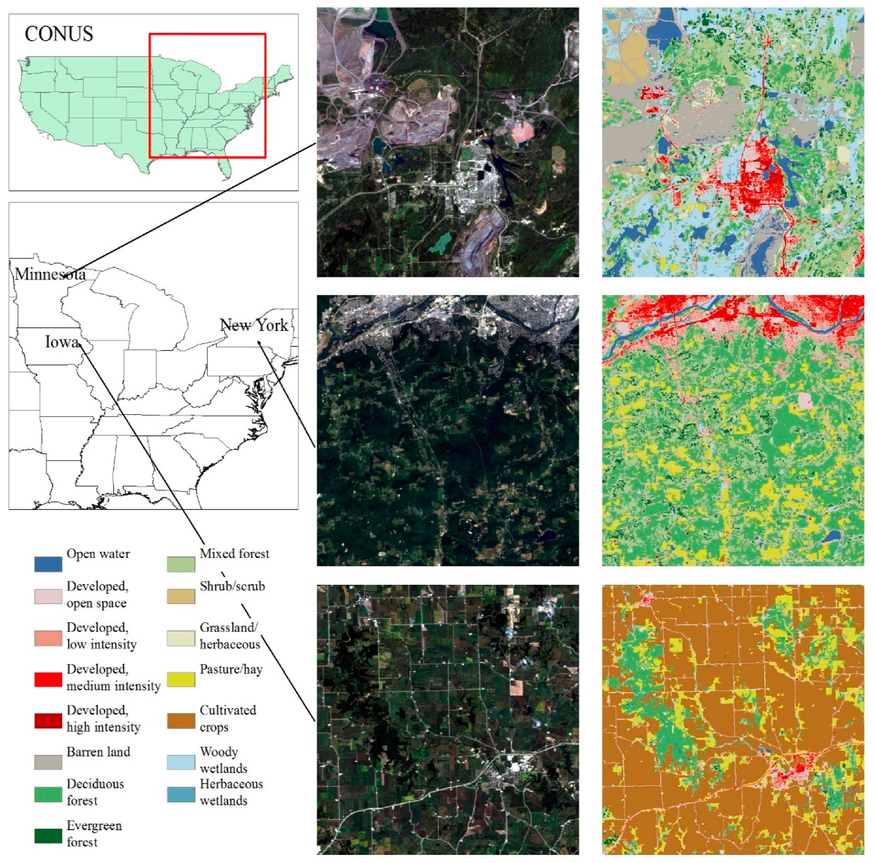
2.3. Study Areas
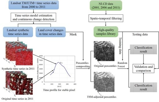
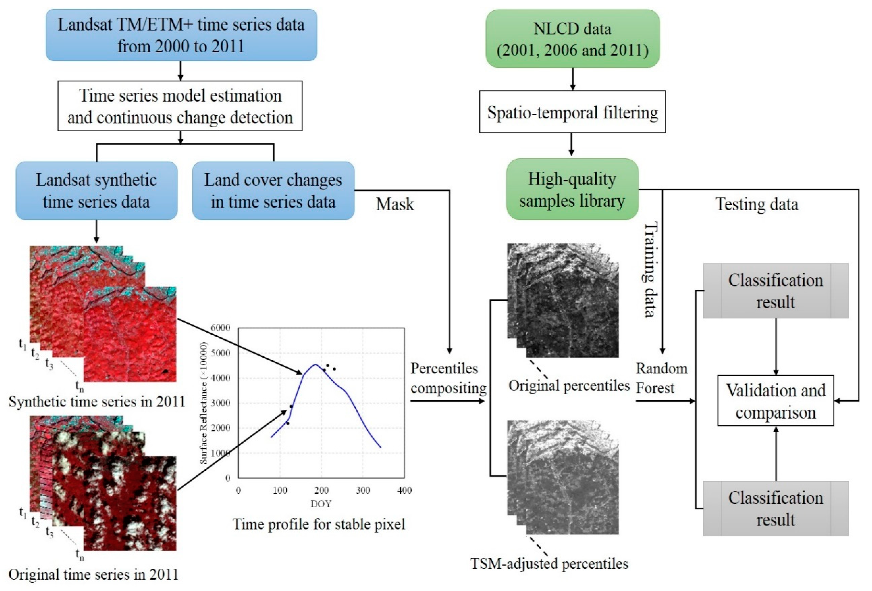
3. Methodology
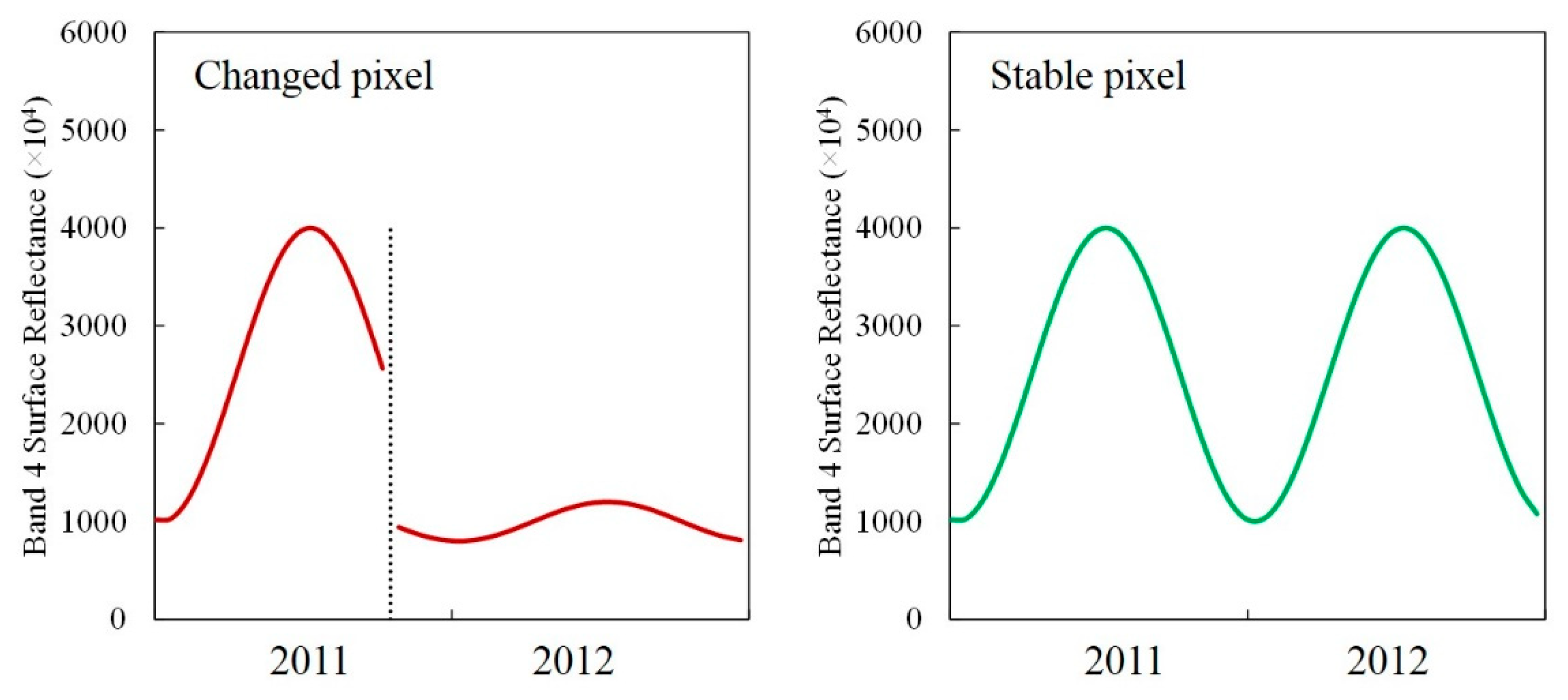
3.1. Development of the Time-Series Model and Continuous Change Detection (CCD)
- x—Julian day
- i—Landsat band i (i = 1, 2, 3, 4, 5, and 7)
- T—number of days of the year (T = 365)
- —constant term that represents the mean for Landsat band i
- , —coefficients of intra-year variation components for Landsat band i
- —coefficient of inter-year variation component (slope) for Landsat band i
- —surface reflectance of Landsat band i on Julian day x obtained using the simple model.
- , —coefficients of the intra-year bimodal variation components for Landsat band i
- —surface reflectance of Landsat band i on Julian day x obtained using the advanced model.
- , —coefficients of intra-year trimodal variation components for Landsat band i
- —surface reflectance of Landsat band i on Julian day x obtained using the full model.
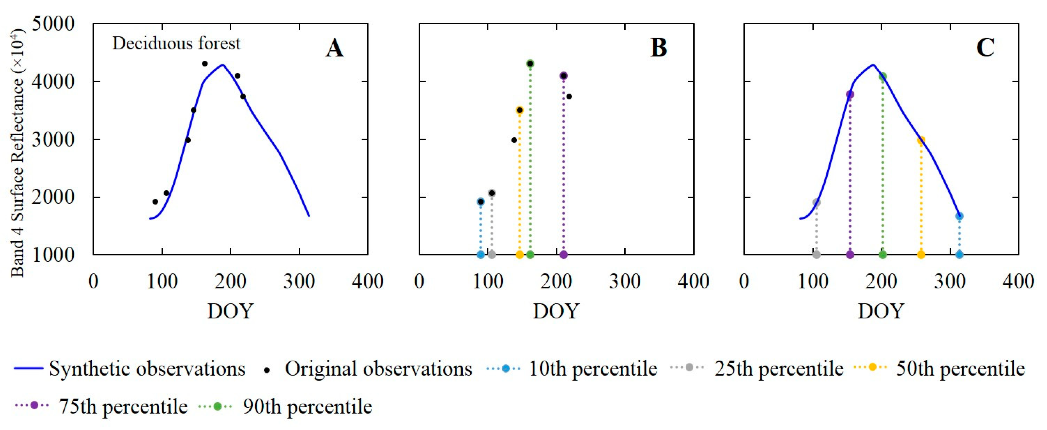
3.2. TSM-Adjusted Percentile Features
3.2.1. Method Used for Calculating Percentiles
3.2.2. Generation of TSM-Adjusted Percentile Features
3.3. Classification Experiment Methodology
4. Results
4.1. Classification of Percentiles Derived from Multispectral Reflectance and NDVI Time Series
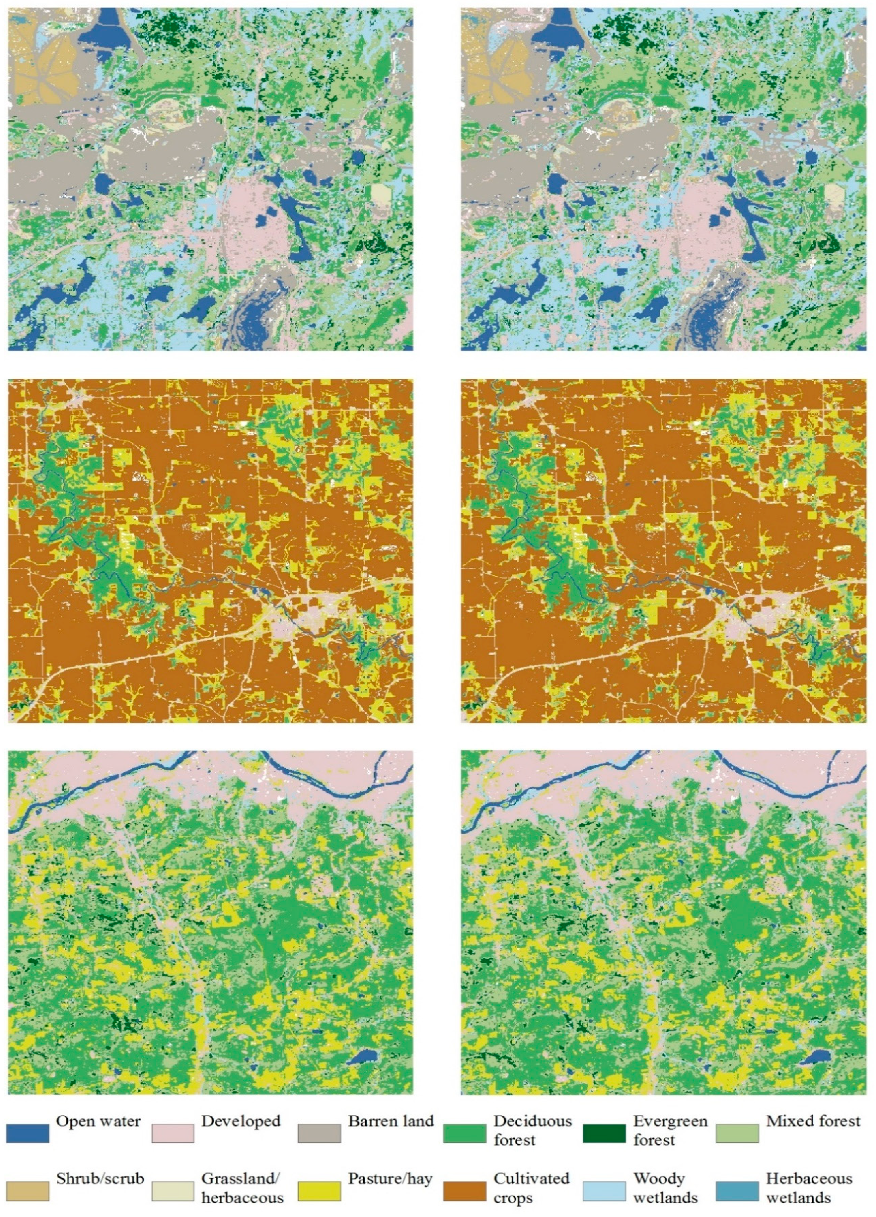
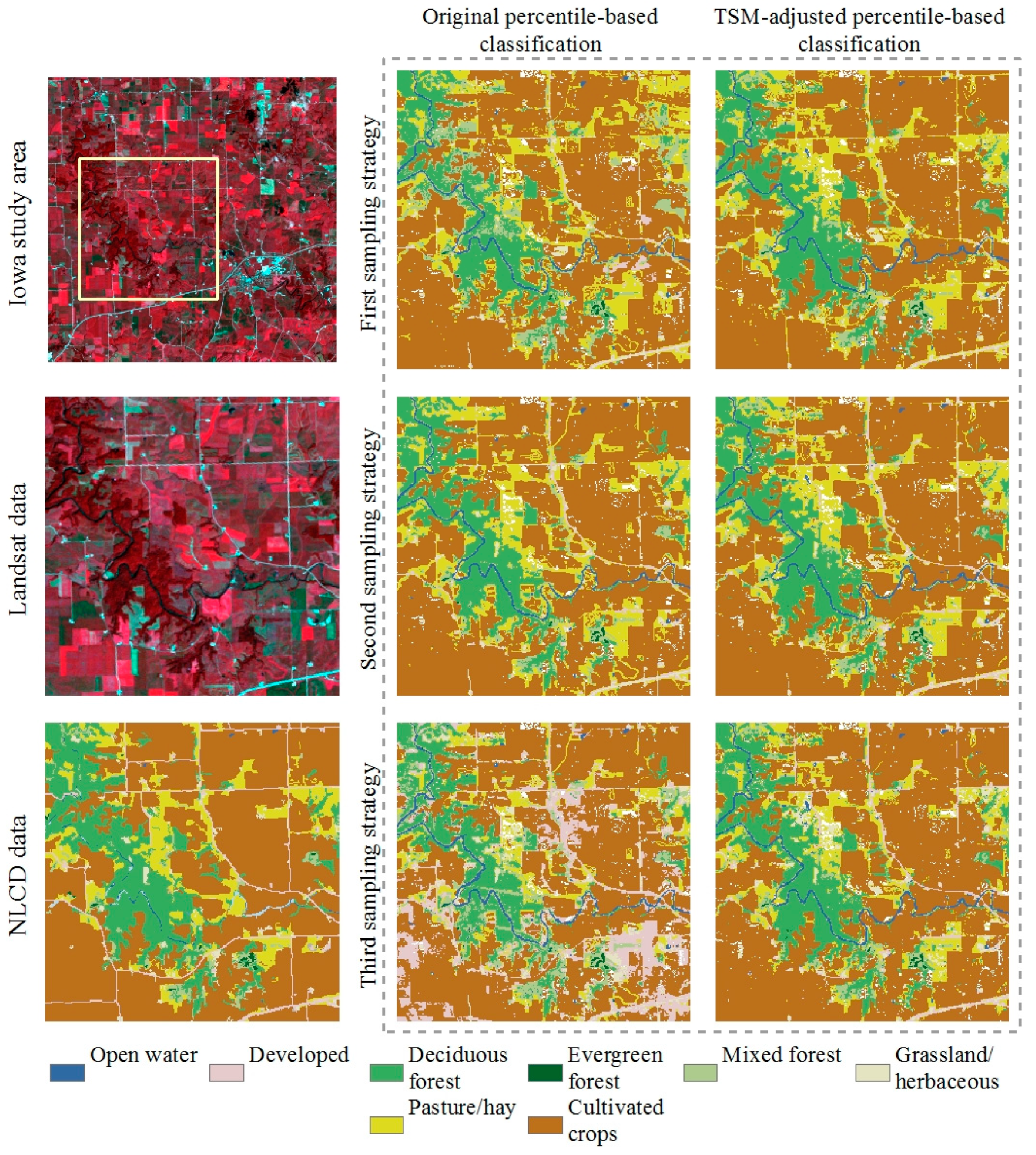
4.2. Spatially Explicit Classification Results
5. Discussion
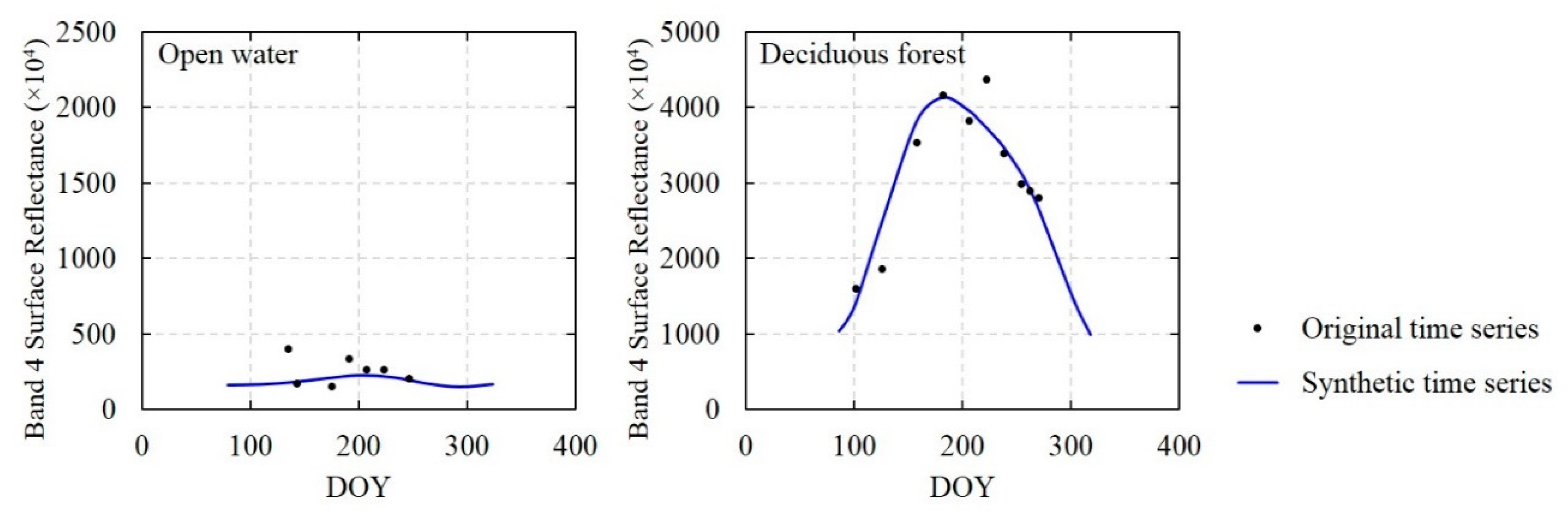
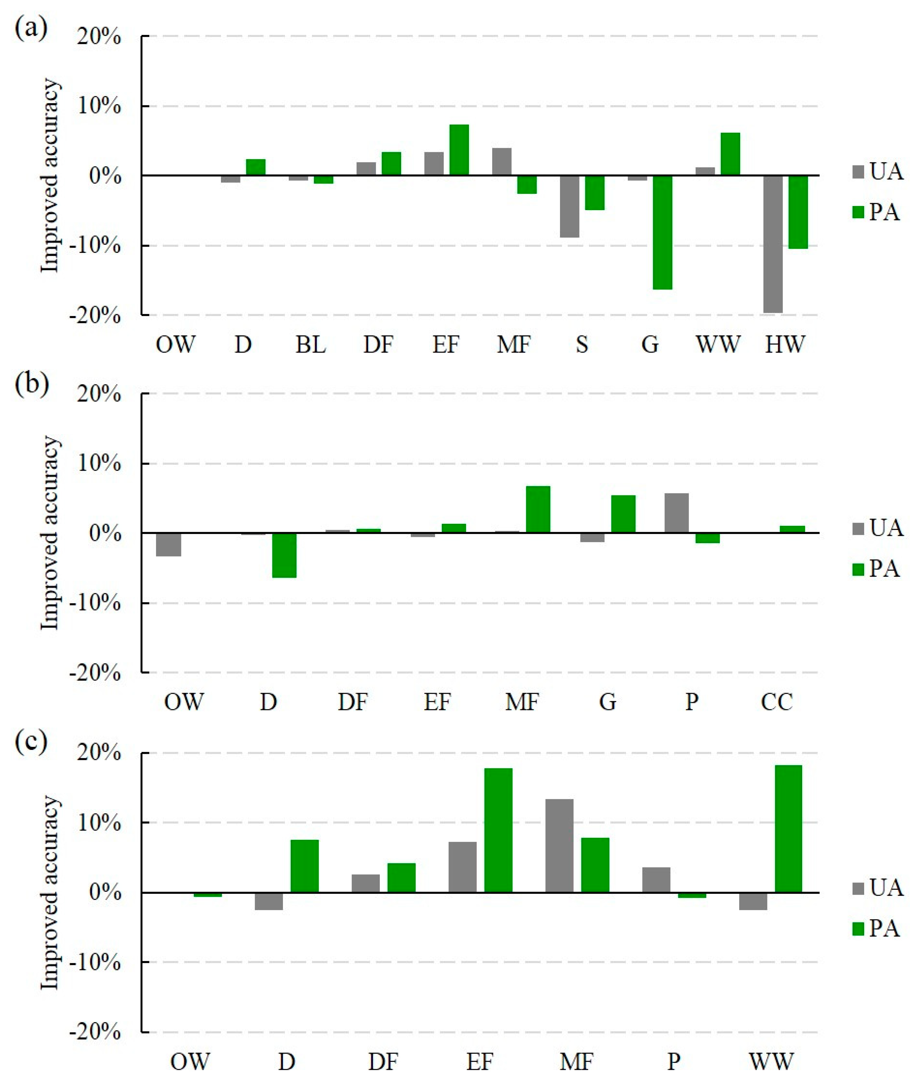
5.1. Effect of Phenological Characteristics
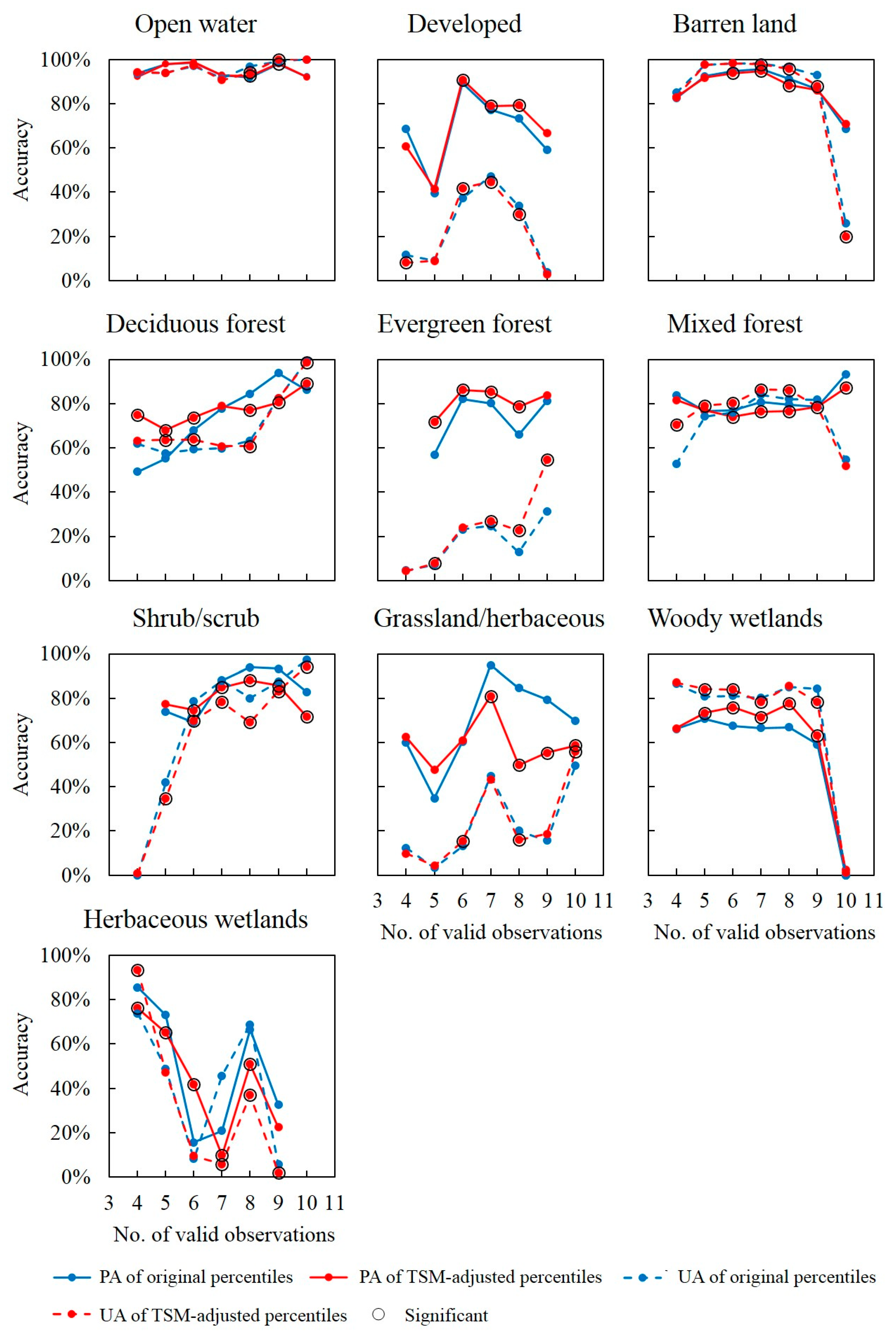
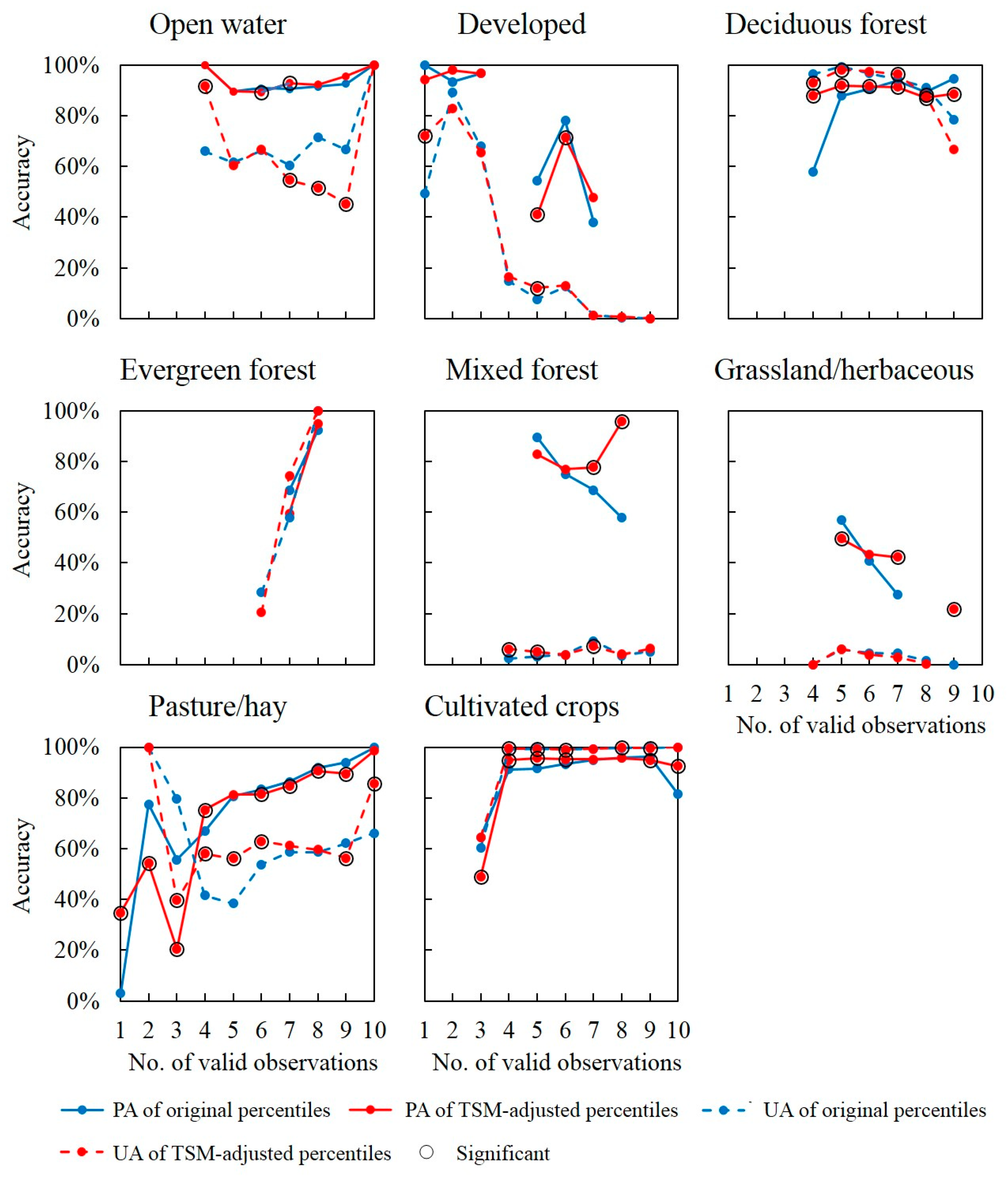
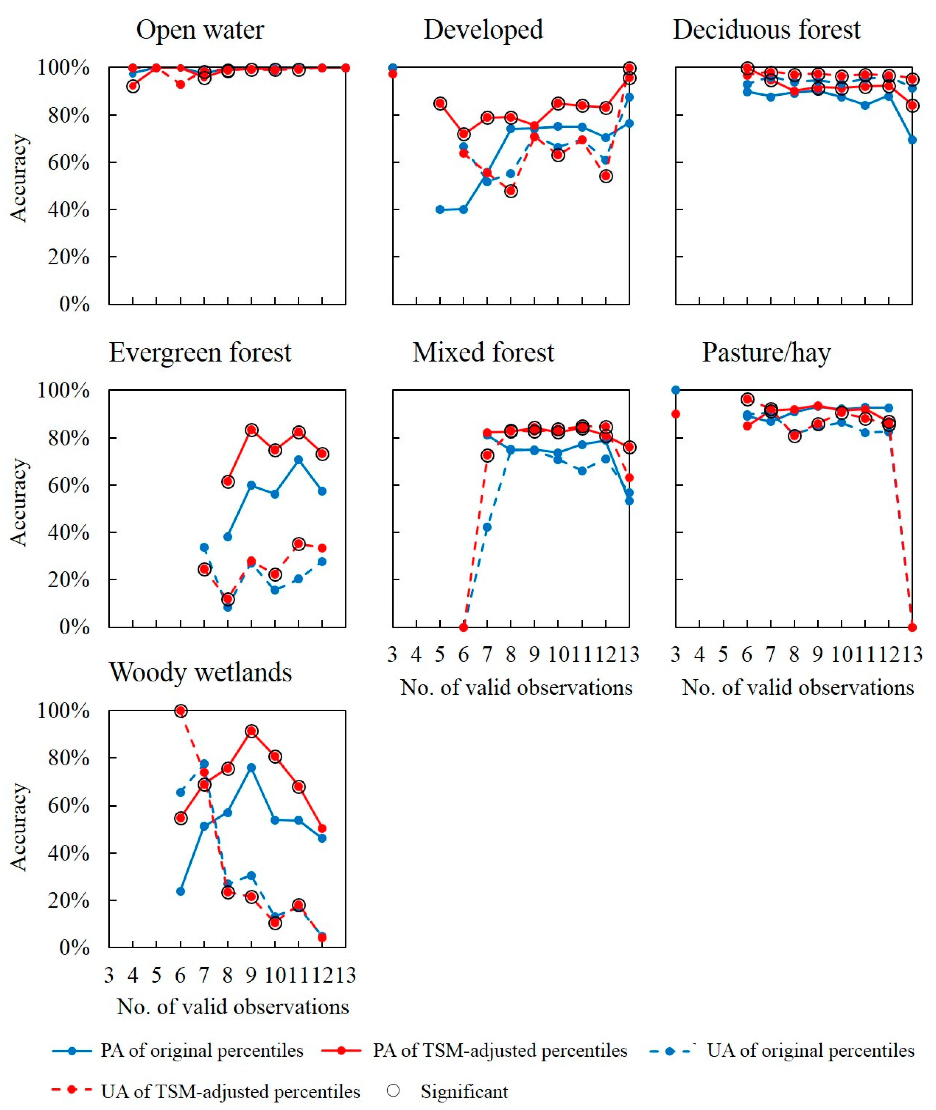
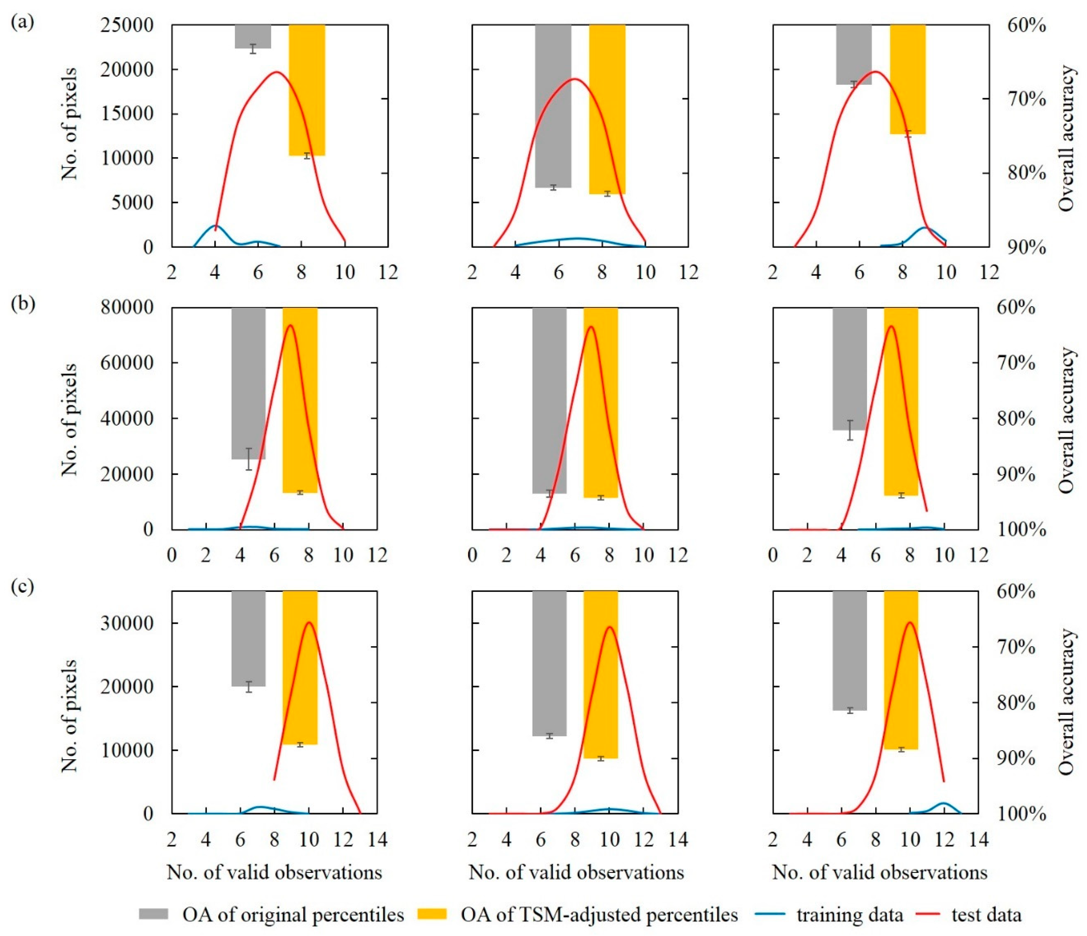
5.2. Effect of the Frequency of Valid Observations
5.3. Effect of Training Data Sampling
6. Conclusions
- (i)
- The land-cover classifications obtained using the proposed TSM-adjusted percentiles had significantly higher overall accuracies than those obtained using the original percentiles.
- (ii)
- The TSM-adjusted percentile features were more effective for forest types with obvious phenological characteristics and with less valid observations.
- (iii)
- The performance of TSM-adjusted percentiles was robust to the training data sampling strategy. The performance difference between the two sets of results was alleviated when using the random sampling across valid observation frequency stratums for each land cover class.
Supplementary Materials
Author Contributions
Funding
Acknowledgments
Conflicts of Interest
References
- Rodriguez-Galiano, V.F.; Ghimire, B.; Rogan, J.; Chica-Olmo, M.; Rigol-Sanchez, J.P. An assessment of the effectiveness of a random forest classifier for land-cover classification. ISPRS J. Photogramm. Remote Sens. 2012, 67, 93–104. [Google Scholar]
- Pereira, H.M.; Ferrier, S.; Walters, M.; Geller, G.N.; Jongman, R.; Scholes, R.J.; Bruford, M.W.; Brummitt, N.; Butchart, S.; Cardoso, A. Essential biodiversity variables. Science 2013, 339, 277–278. [Google Scholar]
- Baker, C.; Lawrence, R.L.; Montagne, C.; Patten, D. Change detection of wetland ecosystems using Landsat imagery and change vector analysis. Wetlands 2007, 27, 610–619. [Google Scholar]
- Masek, J.G.; Huang, C.; Wolfe, R.; Cohen, W.; Hall, F.; Kutler, J.; Nelson, P. North American forest disturbance mapped from a decadal Landsat record. Remote Sens. Environ. 2008, 112, 2914–2926. [Google Scholar]
- Pickell, P.D.; Andison, D.W.; Coops, N.C.; Gergel, S.E.; Marshall, P.L. The spatial patterns of anthropogenic disturbance in the western Canadian boreal forest following oil and gas development. Can. J. For. Res. 2015, 45, 732–743. [Google Scholar]
- Pflugmacher, D.; Cohen, W.B.; Kennedy, R.E. Using Landsat-derived disturbance history (1972–2010) to predict current forest structure. Remote Sens. Environ. 2012, 122, 146–165. [Google Scholar]
- Zhu, Z.; Woodcock, C.E. Continuous change detection and classification of land cover using all available Landsat data. Remote Sens. Environ. 2014, 144, 152–171. [Google Scholar]
- DeFries, R.; Hansen, M.; Townshend, J. Global discrimination of land cover types from metrics derived from AVHRR pathfinder data. Remote Sens. Environ. 1995, 54, 209–222. [Google Scholar]
- Gebhardt, S.; Wehrmann, T.; Ruiz, M.A.M.; Maeda, P.; Bishop, J.; Schramm, M.; Kopeinig, R.; Cartus, O.; Kellndorfer, J.; Ressl, R. MAD-MEX: Automatic wall-to-wall land cover monitoring for the Mexican REDD-MRV program using all Landsat data. Remote Sens. 2014, 6, 3923–3943. [Google Scholar]
- Petitjean, F.; Inglada, J.; Gançarski, P. Satellite image time series analysis under time warping. IEEE Trans. Geosci. Remote Sens. 2012, 50, 3081–3095. [Google Scholar]
- Reed, B.C.; Brown, J.F.; VanderZee, D.; Loveland, T.R.; Merchant, J.W.; Ohlen, D.O. Measuring phenological variability from satellite imagery. J. Veg. Sci. 1994, 5, 703–714. [Google Scholar]
- Azzari, G.; Lobell, D. Landsat-based classification in the cloud: An opportunity for a paradigm shift in land cover monitoring. Remote Sens. Environ. 2017, 202, 64–74. [Google Scholar]
- Hansen, M.C.; Egorov, A.; Roy, D.P.; Potapov, P.; Ju, J.; Turubanova, S.; Kommareddy, I.; Loveland, T.R. Continuous fields of land cover for the conterminous United States using Landsat data: First results from the Web-Enabled Landsat Data (WELD) project. Remote Sens. Lett. 2011, 2, 279–288. [Google Scholar]
- Zhang, H.K.; Roy, D.P. Using the 500 m MODIS land cover product to derive a consistent continental scale 30 m Landsat land cover classification. Remote Sens. Environ. 2017, 197, 15–34. [Google Scholar]
- Wessels, K.J.; Van den Bergh, F.; Roy, D.P.; Salmon, B.P.; Steenkamp, K.C.; MacAlister, B.; Swanepoel, D.; Jewitt, D. Rapid land cover map updates using change detection and robust random forest classifiers. Remote Sens. 2016, 8, 888. [Google Scholar]
- Kovalskyy, V.; Roy, D.P. The global availability of Landsat 5 TM and Landsat 7 ETM+ land surface observations and implications for global 30 m Landsat data product generation. Remote Sens. Environ. 2013, 130, 280–293. [Google Scholar]
- Hermosilla, T.; Wulder, M.A.; White, J.C.; Coops, N.C.; Hobart, G.W. Regional detection, characterization, and attribution of annual forest change from 1984 to 2012 using Landsat-derived time-series metrics. Remote Sens. Environ. 2015, 170, 121–132. [Google Scholar]
- Kennedy, R.E.; Yang, Z.; Cohen, W.B. Detecting trends in forest disturbance and recovery using yearly Landsat time series: 1. LandTrendr—Temporal segmentation algorithms. Remote Sens. Environ. 2010, 114, 2897–2910. [Google Scholar]
- Hamunyela, E.; Verbesselt, J.; Herold, M. Using spatial context to improve early detection of deforestation from Landsat time series. Remote Sens. Environ. 2016, 172, 126–138. [Google Scholar]
- Zhu, Z.; Woodcock, C.E.; Olofsson, P. Continuous monitoring of forest disturbance using all available Landsat imagery. Remote Sens. Environ. 2012, 122, 75–91. [Google Scholar]
- Zhu, Z.; Woodcock, C.E.; Holden, C.; Yang, Z. Generating synthetic Landsat images based on all available Landsat data: Predicting Landsat surface reflectance at any given time. Remote Sens. Environ. 2015, 162, 67–83. [Google Scholar]
- Loveland, T.R.; Dwyer, J.L. Landsat: Building a strong future. Remote Sens. Environ. 2012, 122, 22–29. [Google Scholar]
- Teillet, P.; Barker, J.; Markham, B.; Irish, R.; Fedosejevs, G.; Storey, J. Radiometric cross-calibration of the Landsat-7 ETM+ and Landsat-5 TM sensors based on tandem data sets. Remote Sens. Environ. 2001, 78, 39–54. [Google Scholar]
- Gorelick, N.; Hancher, M.; Dixon, M.; Ilyushchenko, S.; Thau, D.; Moore, R. Google Earth Engine: Planetary-scale geospatial analysis for everyone. Remote Sens. Environ. 2017, 202, 18–27. [Google Scholar]
- Masek, J.G.; Vermote, E.F.; Saleous, N.E.; Wolfe, R.; Hall, F.G.; Huemmrich, K.F.; Gao, F.; Kutler, J.; Lim, T.-K. A Landsat surface reflectance dataset for North America, 1990-2000. IEEE Geosci. Remote Sens. Lett. 2006, 3, 68–72. [Google Scholar]
- Foga, S.; Scaramuzza, P.L.; Guo, S.; Zhu, Z.; Dilley Jr, R.D.; Beckmann, T.; Schmidt, G.L.; Dwyer, J.L.; Hughes, M.J.; Laue, B. Cloud detection algorithm comparison and validation for operational Landsat data products. Remote Sens. Environ. 2017, 194, 379–390. [Google Scholar]
- Zhu, Z.; Woodcock, C.E. Object-based cloud and cloud shadow detection in Landsat imagery. Remote Sens. Environ. 2012, 118, 83–94. [Google Scholar]
- Wickham, J.; Homer, C.; Vogelmann, J.; McKerrow, A.; Mueller, R.; Herold, N.; Coulston, J. The multi-resolution land characteristics (MRLC) consortium—20 years of development and integration of USA national land cover data. Remote Sens. 2014, 6, 7424–7441. [Google Scholar]
- Homer, C.; Dewitz, J.; Yang, L.; Jin, S.; Danielson, P.; Xian, G.; Coulston, J.; Herold, N.; Wickham, J.; Megown, K. Completion of the 2011 National Land Cover Database for the conterminous United States–representing a decade of land cover change information. Photogramm. Eng. Remote Sens. 2015, 81, 345–354. [Google Scholar]
- Zhou, Q.; Tollerud, H.J.; Barber, C.P.; Smith, K.; Zelenak, D. Training Data Selection for Annual Land Cover Classification for the Land Change Monitoring, Assessment, and Projection (LCMAP) Initiative. Remote Sens. 2020, 12, 699. [Google Scholar]
- Wickham, J.; Stehman, S.V.; Gass, L.; Dewitz, J.A.; Sorenson, D.G.; Granneman, B.J.; Poss, R.V.; Baer, L.A. Thematic accuracy assessment of the 2011 national land cover database (NLCD). Remote Sens. Environ. 2017, 191, 328–341. [Google Scholar]
- Zhu, Z.; Wang, S.; Woodcock, C.E. Improvement and expansion of the Fmask algorithm: Cloud, cloud shadow, and snow detection for Landsats 4–7, 8, and Sentinel 2 images. Remote Sens. Environ. 2015, 159, 269–277. [Google Scholar]
- Zhu, Z.; Woodcock, C.E. Automated cloud, cloud shadow, and snow detection in multitemporal Landsat data: An algorithm designed specifically for monitoring land cover change. Remote Sens. Environ. 2014, 152, 217–234. [Google Scholar]
- Friedman, J.; Hastie, T.; Höfling, H.; Tibshirani, R. Pathwise coordinate optimization. Ann. Appl. Stat. 2007, 1, 302–332. [Google Scholar]
- Friedman, J.; Hastie, T.; Tibshirani, R. Regularization paths for generalized linear models via coordinate descent. J. Stat. Softw. 2010, 33, 1–22. [Google Scholar]
- Tibshirani, R. Regression shrinkage and selection via the lasso. J. R. Stat. Soc. Ser. B (Methodol.) 1996, 58, 267–288. [Google Scholar]
- Hansen, M.; Egorov, A.; Potapov, P.; Stehman, S.; Tyukavina, A.; Turubanova, S.; Roy, D.P.; Goetz, S.; Loveland, T.R.; Ju, J. Monitoring conterminous United States (CONUS) land cover change with web-enabled Landsat data (WELD). Remote Sens. Environ. 2014, 140, 466–484. [Google Scholar]
- Breiman, L. Random forests. Mach. Learn. 2001, 45, 5–32. [Google Scholar]
- Belgiu, M.; Drăguţ, L. Random forest in remote sensing: A review of applications and future directions. ISPRS J. Photogramm. Remote Sens. 2016, 114, 24–31. [Google Scholar]
- Zhu, Z.; Gallant, A.L.; Woodcock, C.E.; Pengra, B.; Olofsson, P.; Loveland, T.R.; Jin, S.; Dahal, D.; Yang, L.; Auch, R.F. Optimizing selection of training and auxiliary data for operational land cover classification for the LCMAP initiative. ISPRS J. Photogramm. Remote Sens. 2016, 122, 206–221. [Google Scholar]
- Congalton, R.G. A review of assessing the accuracy of classifications of remotely sensed data. Remote Sens. Environ. 1991, 37, 35–46. [Google Scholar]
- Brooks, E.B.; Thomas, V.A.; Wynne, R.H.; Coulston, J.W. Fitting the multitemporal curve: A Fourier series approach to the missing data problem in remote sensing analysis. IEEE Trans. Geosci. Remote Sens. 2012, 50, 3340–3353. [Google Scholar]
- Ju, J.; Roy, D.P. The availability of cloud-free Landsat ETM+ data over the conterminous United States and globally. Remote Sens. Environ. 2008, 112, 1196–1211. [Google Scholar]
- Kovalskyy, V.; Roy, D.P.; Zhang, X.Y.; Ju, J. The suitability of multi-temporal web-enabled Landsat data NDVI for phenological monitoring–a comparison with flux tower and MODIS NDVI. Remote Sens. Lett. 2012, 3, 325–334. [Google Scholar]


| Study Area | Number of Images from 2000 to 2011 Used for Continuous Change Detection | Number of Images from Target Year 2011 Used for Classification | Spatial Size (Pixels) | Area (km2) | Longitudinal Extent | Latitudinal Extent |
|---|---|---|---|---|---|---|
| Minnesota | 306 | 12 | 489 × 505 | 222.25 | 92.6687°W to 92.4689°W | 47.4744°N to 47.6056°N |
| Iowa | 318 | 14 | 545 × 562 | 275.66 | 91.1540°W to 90.9542°W | 42.2589°N to 42.4026°N |
| New York | 299 | 13 | 541 × 558 | 271.69 | 76.0972°W to 75.8974°W | 41.9614°N to 42.1057°N |
| Land Covers | Minnesota | Iowa | New York |
|---|---|---|---|
| Open water (OW) | 420 | 210 | 210 |
| Developed (D) | 245 | 140 | 280 |
| Barren land (BL) | 700 | - | - |
| Deciduous forest (DF) | 350 | 350 | 630 |
| Evergreen forest (EF) | 182 | 49 | 140 |
| Mixed forest (MF) | 490 | 140 | 420 |
| Shrub/scrub (S) | 280 | - | - |
| Grassland/herbaceous (G) | 140 | 70 | - |
| Pasture/hay (P) | - | 350 | 420 |
| Cultivated crops (CC) | - | 560 | - |
| Woody wetlands (WW) | 560 | - | 161 |
| Herbaceous wetlands (HW) | 70 | - | - |
| Study Area | Original Percentiles-Based Classification | TSM-Adjusted Percentiles-Based Classification |
|---|---|---|
| Minnesota | 81.98% (0.35%) | 82.82%↑(0.33%) |
| Iowa | 93.53% (0.63%) | 94.31%↑(0.38%) |
| New York | 85.99% (0.41%) | 90.05%↑(0.39%) |
| OW | D | BL | DF | EF | MF | S | G | WW | HW | ||
|---|---|---|---|---|---|---|---|---|---|---|---|
| Minnesota | UA | 95.13% | 32.51% | 96.78% | 63.89% | 17.72% | 78.26% | 83.71% | 23.95% | 81.86% | 51.84% |
| PA | 95.86% | 77.42% | 93.03% | 72.18% | 75.32% | 78.74% | 89.31% | 83.28% | 67.53% | 62.89% | |
| OW | D | DF | EF | MF | G | P | CC | ||||
| Iowa | UA | 64.09% | 9.90% | 96.08% | 84.43% | 5.05% | 4.56% | 55.10% | 99.33% | ||
| PA | 90.58% | 71.41% | 90.75% | 90.00% | 73.33% | 37.66% | 86.02% | 94.35% | |||
| OW | D | DF | EF | MF | P | WW | |||||
| New York | UA | 99.24% | 67.36% | 94.46% | 19.29% | 70.29% | 84.43% | 20.43% | |||
| PA | 99.53% | 74.27% | 87.60% | 61.28% | 75.30% | 92.46% | 57.56% |
| OW | D | BL | DF | EF | MF | S | G | WW | HW | ||
|---|---|---|---|---|---|---|---|---|---|---|---|
| Minnesota | UA | 94.96% | 31.57% | 96.12%↓ | 65.84%↑ | 21.14%↑ | 82.25%↑ | 74.90%↓ | 23.20% | 83.02%↑ | 32.17%↓ |
| PA | 95.73% | 79.80%↑ | 91.84%↓ | 75.60%↑ | 82.71%↑ | 76.16%↓ | 84.36%↓ | 66.94%↓ | 73.67%↑ | 52.47%↓ | |
| OW | D | DF | EF | MF | G | P | CC | ||||
| Iowa | UA | 60.70%↓ | 9.57% | 96.54% | 83.84% | 5.37% | 3.24%↓ | 60.79%↑ | 99.29% | ||
| PA | 90.53% | 64.93%↓ | 91.37%↑ | 91.33% | 80.00%↑ | 43.13%↑ | 84.53%↓ | 95.31%↑ | |||
| OW | D | DF | EF | MF | P | WW | |||||
| New York | UA | 99.17% | 64.87%↓ | 97.07%↑ | 26.58%↑ | 83.64%↑ | 88.05%↑ | 17.88%↓ | |||
| PA | 98.97%↓ | 81.90%↑ | 91.77%↑ | 79.01%↑ | 83.12%↑ | 91.73%↓ | 75.75%↑ |
© 2020 by the authors. Licensee MDPI, Basel, Switzerland. This article is an open access article distributed under the terms and conditions of the Creative Commons Attribution (CC BY) license (http://creativecommons.org/licenses/by/4.0/).
Share and Cite
Xie, S.; Liu, L.; Yang, J. Time-Series Model-Adjusted Percentile Features: Improved Percentile Features for Land-Cover Classification Based on Landsat Data. Remote Sens. 2020, 12, 3091. https://0-doi-org.brum.beds.ac.uk/10.3390/rs12183091
Xie S, Liu L, Yang J. Time-Series Model-Adjusted Percentile Features: Improved Percentile Features for Land-Cover Classification Based on Landsat Data. Remote Sensing. 2020; 12(18):3091. https://0-doi-org.brum.beds.ac.uk/10.3390/rs12183091
Chicago/Turabian StyleXie, Shuai, Liangyun Liu, and Jiangning Yang. 2020. "Time-Series Model-Adjusted Percentile Features: Improved Percentile Features for Land-Cover Classification Based on Landsat Data" Remote Sensing 12, no. 18: 3091. https://0-doi-org.brum.beds.ac.uk/10.3390/rs12183091