1. Introduction
During the past 30 years, differential synthetic aperture radar interferometry (DInSAR) has been proven to be an effective technique for studying the deformation processes related to both natural and man-made hazards. DInSAR uses the phase difference (interferogram) between two distinct SAR images acquired at different times over the same scene, permitting retrieval of the projection in the radar line-of-sight (LOS) of the ground deformation that occurred between the two acquisition times, with a centimeter accuracy [
1,
2,
3]. Being an active microwave Earth Observation (EO) technique, space-borne DInSAR represents a very powerful tool for the estimation of ground deformation, thanks to its characteristics of a large spatial coverage, cost effectiveness, and all-weather operability. In this scenario, since the 1992 Landers (California) earthquake, which was the first one detected by interferometric radar images acquired on repeat passes of the ERS-1 satellite [
4], the DInSAR technique has been a viable means of studying earthquakes with observations that are independent of seismology. Interferograms provide information that can be used to model the seismogenic fault that ruptured during an earthquake, thus improving our knowledge of the causative earthquake source.
The scientific literature shows that the number of papers focused on studying earthquakes through DInSAR measurements is continuously increasing [
5,
6]. This is mainly due to the large availability of SAR data archives acquired over time by several satellite systems. We refer in particular to the European Space Agency (ESA) ERS-1/2 and ENVISAT missions, operating at the C-band (a carrier frequency of about 5 GHz), that worked from 1991 to 2011; the Canadian Space Agency (CSA) RADARSAT-1/2, also operating at the C-band since 1995; the Italian COSMO-SkyMed (CSK) and the German TerraSAR-X (TSX) X-band (carrier frequency of about 10 GHz) SAR constellations, both of which were launched in 2007; the Japanese Advanced Land Observation Satellite (ALOS-1/2) L-band (carrier frequency of about 1 GHz) systems launched in 2006 and 2014, respectively.
More recently, the Sentinel-1 (S1) mission, operating since 2014 and belonging to the European Copernicus program, has been acting as a game changer in the EO scenario and natural hazard monitoring. The Sentinel-1 constellation is composed of two twin satellites operating in the C-band (the second satellite was launched in 2016), allowing systematic repeat observations down to 6 days in selected areas of the globe [
7], and thus giving operational support for many scientific and commercial fields, such as natural hazard investigations. The Sentinel-1 constellation is designed to operate with the Terrain Observation by Progressive Scans (TOPS) [
8] technique, which permits ground swaths of about 250 km wide to be imaged. In addition, the S1 acquisitions are intrinsically characterized by small spatial baselines, with an “orbital tube” that has about a 200 m nominal diameter and very accurate orbital information. The Sentinel-1 constellation is therefore particularly suitable for DInSAR applications to detect ground deformation in seismically active regions [
9,
10,
11,
12,
13,
14,
15]. The short repeat time span ensures a quick response in the case of seismic events and fosters the generation of interferograms with a good interferometric quality (because of the short perpendicular and temporal baseline characteristics), even if affecting large areas. These characteristics, along with S1’s global coverage and free and open access data policy, have lowered the barrier to accessing DInSAR data and are continuously increasing the data flow that is supplied all over the Earth, which today reaches about 12 TB per day [
16].
Key issues to be considered while handling Sentinel-1 interferometric SAR data sets are the huge data volume provided by the constellation and the large data size of each acquisition; both make the computing efficiency a crucial aspect when the expected results should be generated immediately after an earthquake. Accordingly, algorithm automation is one of the key aspects required for a successful exploitation of S1 data [
17,
18]. Moreover, to reach high processing performances, appropriate computing infrastructures are needed. Cloud Computing (CC) technologies, which can provide a theoretically “unlimited” number of processing and storage resources [
19,
20], can play a key role in this direction. The use of CC environments can overcome several limitations of in-house solutions, including resource optimization and scaling, performance improvements, complete customization of the computing architecture, and on-demand employment of computing facilities. Moreover, the increasing diffusion of public cloud processing services at reduced costs and the availability of EO data catalogs directly on-the-cloud are also pushing towards the adoption of such technologies in EO scientific contexts. For instance, Amazon Web Services (AWS), through the Amazon Simple Storage Service (S3), is making the full Sentinel-1 and Sentinel-2 data archives available [
21], as well as Google, with their Earth Engine framework [
22]. More recently, the European Commission set up the Data and Information Access Services (DIAS) [
23], where satellite data belonging to the Copernicus EO program and processing facilities are co-located to reduce the transfer time during processing.
In this context, some operational services based on Sentinel-1 DInSAR processing data have already been set up [
24,
25,
26,
27,
28]. Considering the relevance of satellite interferometric analysis for the study and monitoring of seismic hazards, as well as the availability of the Sentinel-1 constellation characterized by a high operational reliability, in this work, we present the development and implementation of an automatic and unsupervised tool for the systematic generation of S1 DInSAR coseismic displacement maps, in addition to the associated wrapped interferograms and coherence maps, at a global scale. The S1 short revisit time and the global spatial coverage permit us to theoretically generate any possible coseismic interferogram relevant to every earthquake capable of causing measurable surface deformation. The tool is triggered by the most significant (according to a set of defined thresholds) seismic events registered by the online global catalogs, such as those provided by the United States Geological Survey (USGS) [
29] and the Italian National Institute of Geophysics and Volcanology (INGV) [
30]. Then, our system, after automatically querying and retrieving the S1 data from the available online catalogs, generates pre-, co-, and post-seismic deformation maps by exploiting a proper CC environment. Finally, the retrieved information is stored and organized in a global DInSAR earthquake database that is progressively made openly available to the Solid Earth community through the European Plate Observing System (EPOS) [
31] Research Infrastructure. This allows the EO community to obtain coseismic DInSAR displacement maps and the related information in a short time frame and nearly anywhere in the world, thus significantly improving the capability for studying the seismic zones at a global scale.
The paper is organized as follows. First, we present a general description of the workflow of the unsupervised tool that automatically generates coseismic interferograms and displacement and coherence maps by using Sentinel-1 SAR data. Processing details and product specifications are also provided. Then, several examples of the results achieved through the implementation of the proposed tool are shown. In the last part, we present a discussion on the obtained results, the main limitations of the implemented system, and the future developments through which the tool can be extended. In the final section, some conclusive remarks are discussed.
2. Automatic Tool for the Generation of Coseismic Sentinel-1 DInSAR Products
In this section, we present the rationale and workflow of our tool, which can be employed for the automatic generation of S1 DInSAR displacement maps (and the associated interferograms and coherence maps) following a seismic event. Details on the specific parameters and thresholds used for the implementation of the proposed workflow are also provided.
The implementation allows us to set up an operational service that automatically generates coseismic Sentinel-1 DInSAR products. Moreover, the same tool has been run for the historical S1 data archive to populate a global database of DInSAR-based displacement maps and related information that can be made available to the scientific community.
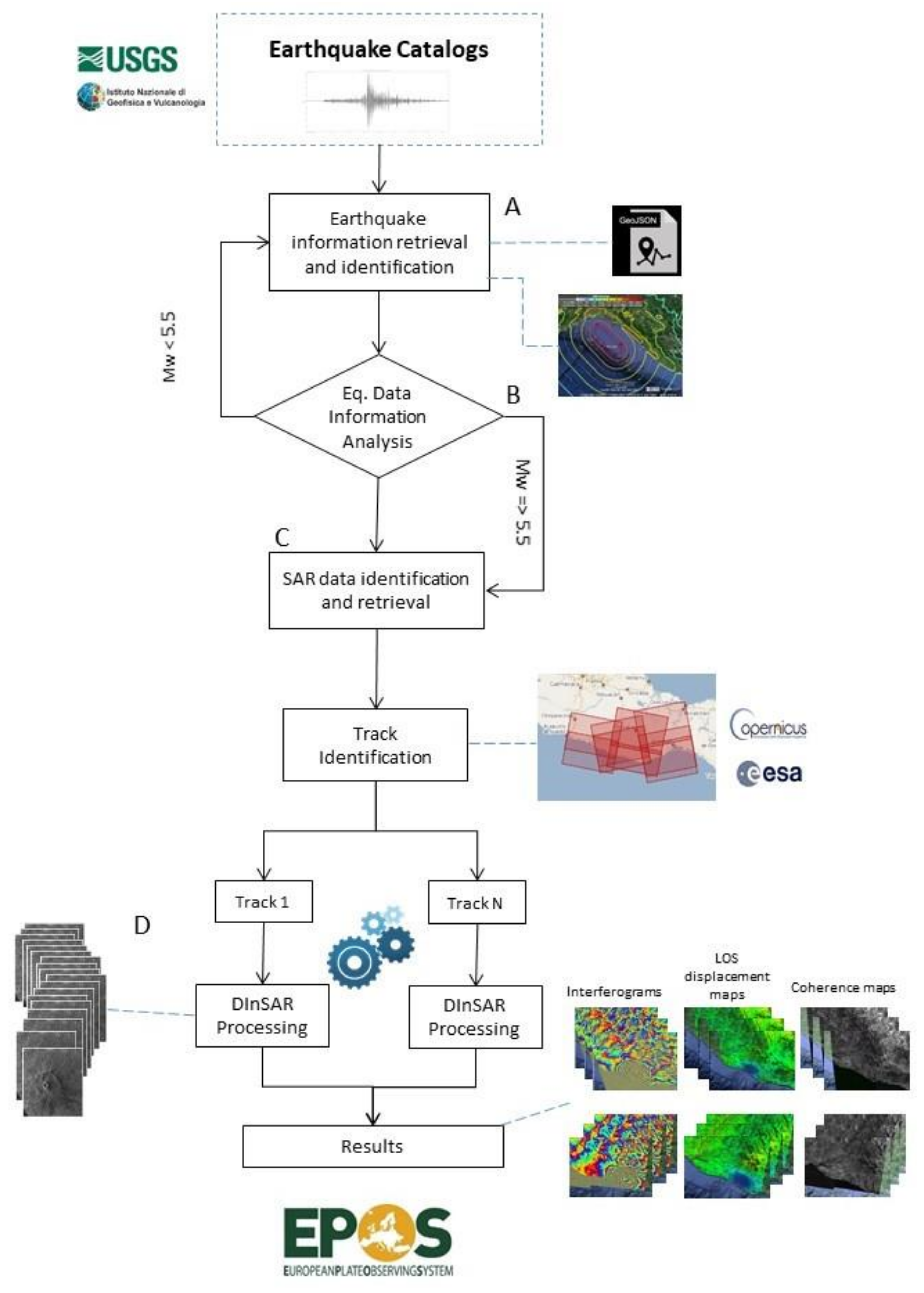
Figure 1 shows a block diagram of the tool procedure, which is described in detail in the following section.
2.1. Earthquake Information Retrieval and Identification
When an earthquake occurs, seismic information (i.e., magnitude, hypocenter location, time, etc.) is collected and made available through online public catalogs. These catalogs are managed by the main national and international geophysical institutions, including USGS [
29] and INGV [
30].
Such institutions provide information related to all of the seismic events that their networks are able to retrieve. The seismic parameters’ accuracies depend on the network density and spatial extension, but in general, the catalogs are capable of providing global seismic information. Catalogs are updated in real time at every occurrence of a new seismic event, thus making them a complete source of information for studying earthquakes at local and global scales. Moreover, the seismic parameters are searchable through a visual interface, as well as a machine-to-machine Access Program Interface (API). To guarantee interoperability, the catalogs generally provide earthquake information in open standard formats. One of the most used is the geoJSON format, which represents geographic elements along with attributes based on JavaScript Object Notation.
Once an earthquake with a significant magnitude occurs and its characteristics are calculated and published in one of the available online catalogs, our procedure starts (Block A,
Figure 1). The USGS earthquake catalog can be exploited in order to retrieve earthquake information worldwide. Moreover, specifically for the Italian territory, seismic information can be retrieved from the INGV data catalog. For national purposes, it is preferable to exploit local catalogs to rely on more accurate magnitude and localization estimates. This also allows us to perform ad hoc computations for very shallow and low-magnitude (<5.5 M
w) earthquakes in Italy.
In general, a query on the earthquake parameters can be made in different ways, according to the available catalog features. Most advanced catalogs provide continuous updates and alerts through specific subscriptions to RDF Site Summary (RSS) feeds. This implies not developing any specific procedure for catalog querying (the information is simply provided by the catalog in an automatic way); however, it makes the earthquake information retrieval completely dependent on the catalog used (because not all of them provide such features), thus limiting the tool’s portability.
On the contrary, it is possible to poll the desired catalogs to search for the required information. This provides more flexibility at the expense of defining a procedure for catalog querying and polling. In general, the last option is more customizable and is more suitable for inhomogeneous catalogs. To keep the system as general as possible, a systematic query is carried out every 15 min to identify possible new earthquakes. Note that, since the generation of S1 DInSAR displacement maps strongly depends on the S1 data availability (which has, as a minimum, a 6-day repeat), it is not mandatory to retrieve the earthquake information in real time.
Independent of the method used for querying the earthquake catalogs, the information to be retrieved consists of the magnitude, epicenter location, hypocenter depth, and time of the event. They are used to identify the SAR data to be employed to generate the coseismic interferogram and are even used to obtain a preliminary indication of the earthquake’s potential to induce surface deformation, thus indicating whether to trigger related DInSAR processing.
The magnitude represents the energy released by the earthquake and is provided as an absolute number. The epicenter location is usually provided as the latitude and longitude, both in degrees and with respect to a WGS84 reference datum, while the depth is given in kilometers beneath the surface. The earthquake occurrence time is provided in milliseconds or the UTC format [
29]. In addition to the aforementioned mandatory parameters for the proposed procedure, other parameters of interest could be relevant. They include the textual geographic name of the area affected by the earthquake (to have a common human readable name associated with the event), as well as the focal mechanism that could be used for further earthquake studies and interpretations.
2.2. Earthquake Data Information Analysis
Once collected, the retrieved earthquake descriptive parameters are evaluated to drive the subsequent interferometric processing. At a defined depth, the induced surface deformation is related to the magnitude, which then represents a key parameter for describing an earthquake. However, earthquakes of the same magnitude but at different depths can produce significantly different deformation on the Earth’s surface. Therefore, once an earthquake occurs, it first has to be evaluated whether it can induce DInSAR-detectable surface deformation. In our workflow, this evaluation is performed in Step B of
Figure 1. This evaluation is needed to avoid running the subsequent DInSAR processing for an event that we already know is very unlikely to produce detectable ground deformation.
At this stage, empirical considerations are carried out, based on previous experiences and the literature [
9,
32,
33,
34,
35]. In particular, in this work, we propose a simple classification of magnitude (specifically the moment magnitude M
w) with respect to the depth, identifying classes of magnitude that can reasonably produce surface deformation at a defined maximum depth. This is done starting from M
W 5.5 according to
Table 1.
Moreover, specifically for the Italian territory for which the seismic information from the INGV data catalog is exploited, information on earthquakes with a magnitude M
w in a range between 4.0 and 5.5, with a depth of less than 20 km, is also collected. This could be particularly useful for volcanic areas that can be affected by very shallow earthquakes of a moderate magnitude [
36,
37].
Only the earthquakes that respect the proposed classification subsequently undergo DInSAR processing. The possibility to detect the induced ground deformation also depends on the radar sensor carrier frequency; however, since the proposed tool is meant to be used with Sentinel-1 data, this discussion is left to future work. Following the first evaluation of the detected earthquake, further refinements are carried out, mainly to identify those earthquakes above the threshold for DInSAR processing. First of all, only those earthquakes that are located on land or at a distance smaller than a defined threshold (in km) from the coastline are selected. This is primarily because DInSAR can only detect deformation on land. Moreover, even epicenters on water can produce deformation on land if they are close enough to the coastline. Therefore, the threshold on the distance is defined upon a consideration of the magnitude and depth (that determine the expected area on the surface affected by deformation), and the satellite swath width. We set up a maximum allowed distance of the epicenter from the closest coastline (see
Table 1), depending on the magnitude. This is based on previous work that showed the possibility to detect ground deformation in the case of significant earthquakes (M
w > 7.0) whose epicenter is located in the sea, but relatively close to land [
10,
13].
Furthermore, there is the possibility that multiple earthquakes, which satisfy the previous selection criteria, occur in the same area, thus implying a possible duplication of DInSAR processing; this behavior should clearly be avoided to optimize the use of the computing resources. This means that the occurrence of a new earthquake in an area where DInSAR processing is already in place (because of a previous earthquake) does not imply the start of an additional run of the procedure. A particular case, which is also taken into account, is represented by the occurrence of a new earthquake within a satellite repeat cycle period, which is the typical case of aftershocks, i.e., before the generation of the coseismic interferogram related to the main shock. For this scenario, the key aim is to quantify how “close” two epicenters are, in order to consider whether they are already being covered by other DInSAR procedures that are in progress. To do this, a threshold on the maximum distance between the epicenter location and the area covered by the current DInSAR processing is imposed. We set the maximum distance between two epicenter locations to be considered as falling in the same region of an already running DInSAR process to 50 km.
We applied the proposed selection criterion not only during the occurrence of new earthquakes, but also to the entire USGS catalog collected from January 2015 up to July 2020, which corresponds to the Sentinel-1 main data availability.
2.3. SAR Data Identification and Retrieval
The earthquake parameter evaluation is followed by the selection of the Sentinenl-1 Single Look Complex (SLC) data, i.e., the SAR images in the azimuth-range radar coordinates, to be used for carrying out the DInSAR processing. For the selected earthquakes (according to the previously described procedure), an automatic query of the available SAR data catalogs is performed (Block C,
Figure 1). This query permits the identification of all the satellite tracks of Sentinel-1 level-1 data (SLC images), from both ascending and descending passes, that totally or partially cover the area likely affected by the earthquake-induced deformation. The query is performed over an area whose extension depends on the earthquake magnitude and depth. In particular, centered on the epicenter location, a search area is set according to classes of the magnitude, depth, and spatial extension, based on empirical considerations of the expected surface deformation, following
Table 1. In general, large magnitude earthquakes induce deformation at a wide spatial scale. While the area extension should not have less of an impact on satellites characterized by wide swaths (as, for instance, the Sentinel-1 one), it is nonetheless fundamental for ensuring the highest possible coverage of the area affected by deformation. The subsequent processing is carried out by merging all of the S1 data slices belonging to the same track that covers the deformed area. Once the tracks covering the earthquake area have been identified, the system retrieves all of the available SAR data up to 36 days before the event (which generally means considering three to six images, depending on the actual repeat time), in order to allow the generation of the coseismic interferograms. In case no pre-event images are available in the investigated interval, at least one image is searched in a larger time span.
The data retrieval and subsequent DInSAR processing remain active up to 36 days after the event, in order to generate several co- and post-seismic interferograms. In this way, the system can assure data redundancy, which can be very helpful for identifying an undesired phase signal. The proposed tool thus has the ability to continuously and automatically identify if a new satellite image covering the processed area is available, download the new images for every track, and update the processing to generate new (updated) DInSAR results.
The SAR data are retrieved from the SciHub catalog [
38], which is the official Sentinel-1 data repository, and the Alaska Satellite Facility (ASF) [
39], which is available on the Cloud.
2.4. Sentinel-1 DInSAR Processing
Once the relevant pre-event data have been downloaded, the subsequent DInSAR processing is carried out by using a portion of the in-house implemented Sentinel-1 Parallel Small BAseline Subset (P-SBAS) [
18] processing chain (Block D,
Figure 1). Instead of performing the whole SBAS processing, the P-SBAS chain is exploited up to the interferogram generation step, so that the processing can benefit from the implemented parallelization strategies.
To highlight some of the features of the P-SBAS processing chain, we first remark that the processing is carried out at the Sentinel-1 full spatial resolution up to interferogram generation. At this step, for generating the differential interferograms, a multilook operation is implemented with 20 looks along the range direction and 5 along the azimuth one, corresponding to about an 80 × 80 m pixel size on the ground. Moreover, the original differential interferograms are generated by exploiting the Enhanced Spectral Diversity (ESD) method [
40]. The ESD approach estimates the residual azimuth shifts among TOPS data pairs by evaluating the phase discontinuities in the overlapping regions between azimuth-adjacent bursts. The mean standard deviation value of the phase differences computed with the ESD algorithm implemented within the P-SBAS chain is around 1 × 10
−3 samples (as described in [
18]), so that a high quality of the interferometric products is guaranteed.
Furthermore, to retrieve the displacement information, a phase unwrapping procedure is applied. The Minimum Cost Flow (MCF) algorithm [
41], which corresponds to the state of the art for single interferogram phase-unwrapping, is exploited. The MCF algorithm is performed on a set of pixels, which are selected by setting a threshold of 0.25 for the interferometric coherence.
To speed up the DInSAR processing and to benefit from a scalable computing environment, our tool has been implemented within a Cloud Computing (CC) platform, which has recently been demonstrated to effectively process large amounts of EO satellite data [
18,
19]. Indeed, nowadays, several CC platforms [
21,
22,
23] are hosting large archives of EO data, making them freely available to their users. Such data archives, which are highly reliable, allow us to avoid downloading data to in-house facilities, thus reducing the whole processing time, as well as the cost of local data storage. Secondly, although processing a single DInSAR product set is not extremely computationally demanding nowadays, the scalability provided by the CC platforms is crucial for processing several tracks covering the same earthquake in parallel, as well as several earthquakes that can occur close in time, allowing a general reduction of the processing cost and an increase of the service effectiveness (particularly when the service is primarily addressed to serve civil protection authorities).
The CC infrastructure benefits for the EO field can be synthetized as follows: (1) providing access to near-real time and historical data; (2) combining data and processing in one location; (3) allowing on-demand processing; (4) providing processing that is scalable, sizeable, reliable, and secure.
We implemented the presented automatic tool by exploiting the Amazon Web Service EC2 services. In particular, we configured a customized Amazon Machine Image (AMI) containing the operating system (Linux 4.4.0-1040-aws x86_64), the workflow manager (which performs the earthquake identification, the data download, the P-SBAS processing scheduling, and the storage and final result dissemination), and the software needed for the Sentinel-1 P-SBAS processing, which is composed of a set of scripts coded in different languages, such as Interactive Data Language (IDL), Fortran, and C. The characteristics of the exploited AWS instance are provided in
Table 2.
Although the specific implementation we present exploits AWS resources, the workflow manager is coded in Linux Bash, which avoids the installation of any additional software, tools, or libraries, and finally makes it highly portable to any Linux-based system.
The Sentinel-1 P-SBAS processing strategy is performed according to [
19]. In particular, depending on the specific P-SBAS step to be executed, and exploiting the intrinsic TOPS burst granularity, different parallel jobs are distributed among the multiple cores of the AWS machine, optimizing the use of computing resources (CPUs, RAM occupation, and I/O bandwidth). Error control, as well as synchronization mechanisms, are also implemented. Moreover, the processing of the different tracks is carried out in parallel, while their actual execution depends on the available computing resources and on the effective temporal acquisition of the SAR data. Processing prioritization of the different tracks on the basis of the post-event acquisition time has been implemented (according to a First-Come-First-Served policy). However, by disposing of sufficient computing facilities, it is possible to perform the different Sentinel-1 P-SBAS processing tasks in parallel.
2.5. Output and Results
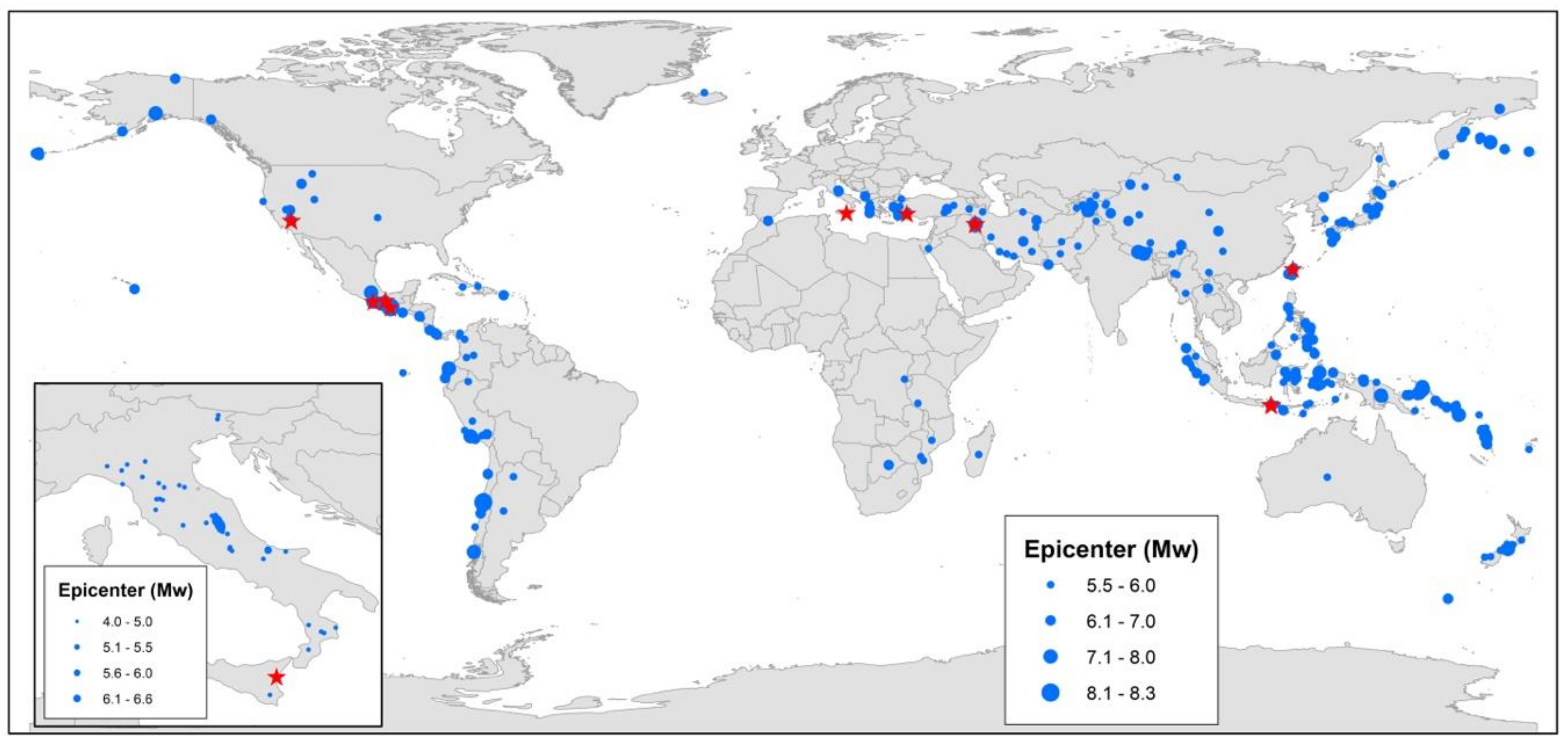
We selected 460 global earthquakes that occurred from January 2015 to 6 Jul 2020 and satisfied
Table 1 and previous criteria for DInSAR processing. From these, 333 locations were processed to avoid duplication. A further 50 actual locations were considered in Italy, due to the differently used thresholds.
Figure 2 shows the location of the identified earthquakes; in red are the events that are presented in the following experimental results section.
For all of the identified locations, the tool provided wrapped interferograms and displacement maps (unwrapped interferograms converted in centimeters) in the satellite LOS. For the latter, automatic identification of the reference point was implemented based on the epicenter location, the footprint, and the spatial coherence. The spatial coherence and unit LOS vector for each pixel are also provided, for signal quality analysis and for further post-processing investigation.
The generated DInSAR wrapped interferograms were filtered with a power spectral filter [
42] with an exponential smoothing factor of 0.5, in order to reduce the phase noise. Any other data filters and interpretations were left to the user needs and skills.
The output data were generated according to the file formats defined within the European Plate Observing System (EPOS) [
31] Research Infrastructure, to make them standardized and interoperable. In particular, the actual measurements are provided as geocoded raster floating point matrices packed within a GeoTIFF envelope to ensure product portability. The datum used was WGS84. Product previews are provided in PNG format. The metadata follow the ISO 19115 standard with custom tags for describing the DInSAR specific parameters, i.e., baselines, reference acquisitions, etc. More details on the interferometric product formats and metadata are provided in the
Supplementary Material.
Once generated, the results and final products, together with the relevant metadata and previews, were uploaded to the EPOS Satellite Data community repository (TCS-SATD) [
31], which is hosted by the Geohazards Exploitation Platform (GEP) [
24]. Presently, the EPOS catalog population is a work in progress. Uploaded products (and metadata) can be anonymously accessed through the EPOS geo-portal, which allows users to perform geographic queries and visualize a preview of the retrieved results over a background map. Moreover, it is also possible to visualize other communities’ products that can be of interest for DInSAR data previews (i.e., fault traces, available GNSS stations, seismicity, etc.). A product download is freely available to all those in the EPOS, as well as GEP registered users, according to a Creative Commons (CC-BY) license.
3. Experimental Results
We generated the coseismic interferograms and corresponding displacement and coherence maps relevant to 460 earthquakes identified according to the procedure detailed in
Section 2 and, in particular, to
Table 1.
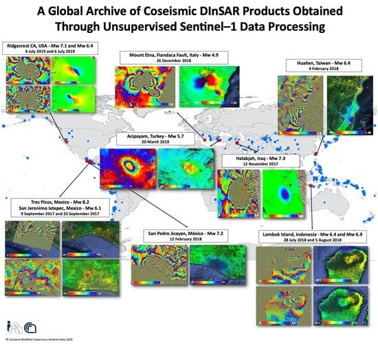
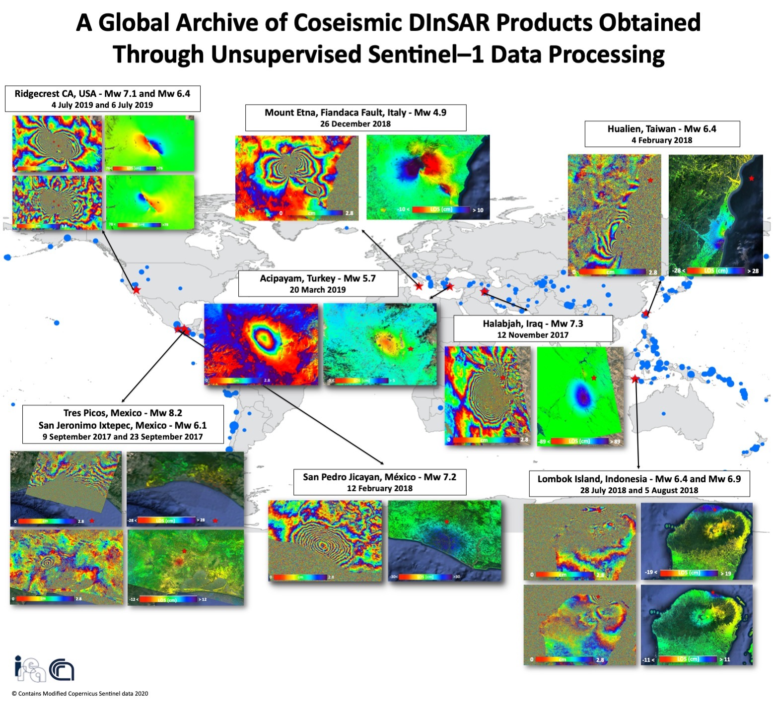
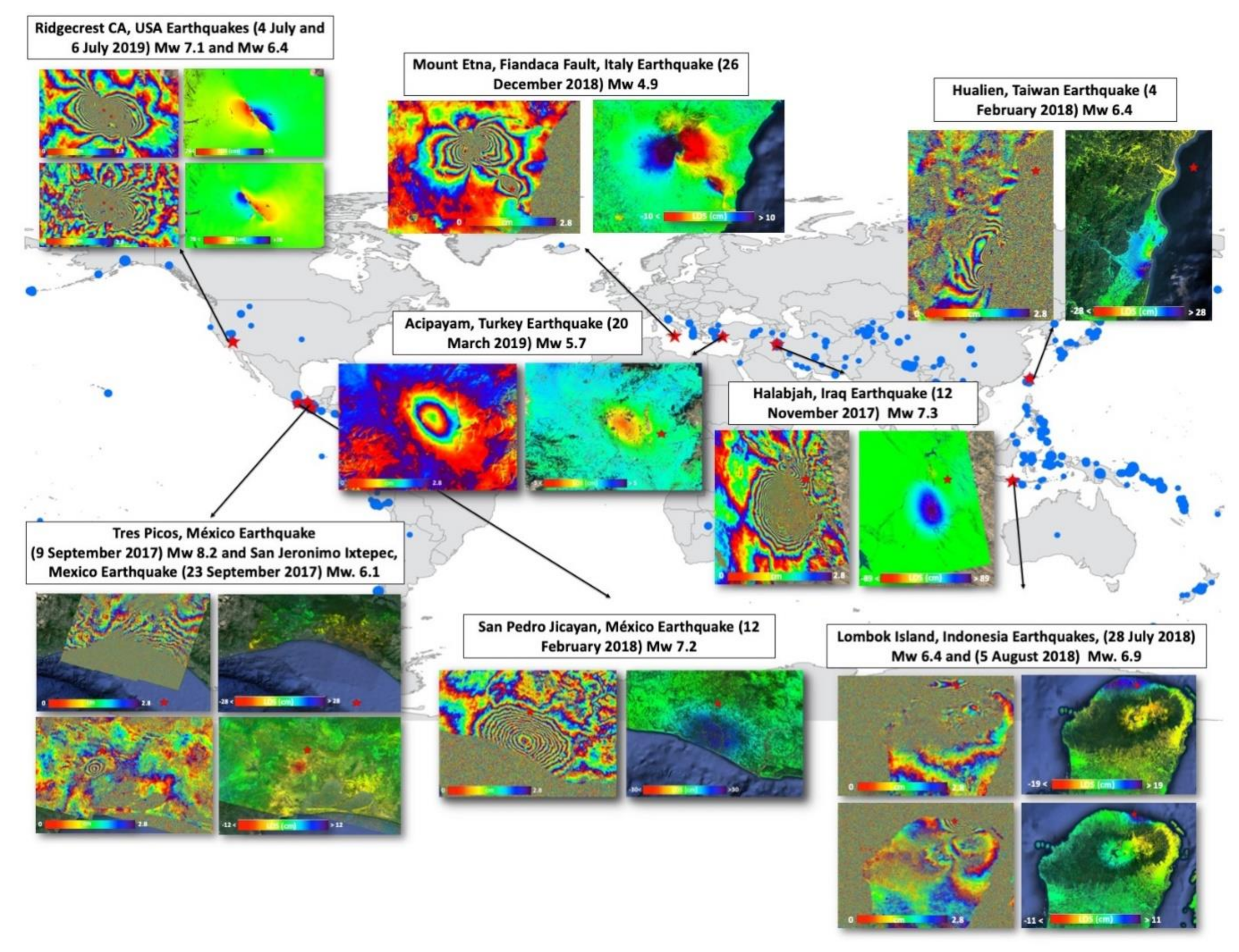
Figure 3 shows an overview of the results obtained across the Earth. These examples, as better detailed in the following text, prove the effectiveness of the implemented automatic and unsupervised DInSAR processing procedure for studying earthquakes, and permit us to show the adopted processing optimization strategies reported in
Section 2.2 and
Section 2.3. In particular, we present coseismic interferograms and displacement maps relevant to events with the following characteristics: several earthquakes occurred within a single interferogram time interval, such as for the Ridgecrest (CA, USA) case (see
Section 3.1); earthquakes and volcanic eruptions as for the Mt. Etna (Italy) case (
Section 3.2); earthquakes of a small magnitude, as with the Acipayam (Turkey) case (see
Section 3.3); earthquakes that occurred in the same area, but in different periods, as for the southern South Mexico and Lombok Island (Indonesia) cases (
Section 3.4); significant earthquakes that induced spatially large deformation patterns, as found with the southern Mexico and Halabjah (Iraq/Iran) cases (see
Section 3.5); finally, earthquakes localized in the sea, as in the Hualien (Taiwan) case (see
Section 3.6).
3.1. Several Earthquakes in the Same Interferogram
On July 2019, a seismic sequence struck the Ridgecrest area, California (USA). In particular, two major earthquakes occurred; the first one on 4 July 2019 with a M
w 6.4 and a depth of 10.5 km, and the second one just two days after (6 July 2019), with a M
w 7.1 and a depth of 8.0 km. The predominant mechanism of the M
w 6.4 earthquake was a left lateral strike-slip fault movement along a NE–SW trending fault which was conjugated with the M
w 7.1 earthquake fault that broke the Earth’s surface and involved a right-lateral strike-slip along a NW–SE trending fault [
43].
Due to the very short time interval between the two events and the S1 satellite’s repeat cycle period, it was possible to detect both seismic events in the same interferogram (and related displacement map).
Moreover, thanks to our developed DInSAR procedure (see
Section 2.2), no processing duplication occurred and only one interferogram was automatically generated following the occurrence of the first earthquake, thus avoiding the start of an additional but useless run of the procedure.
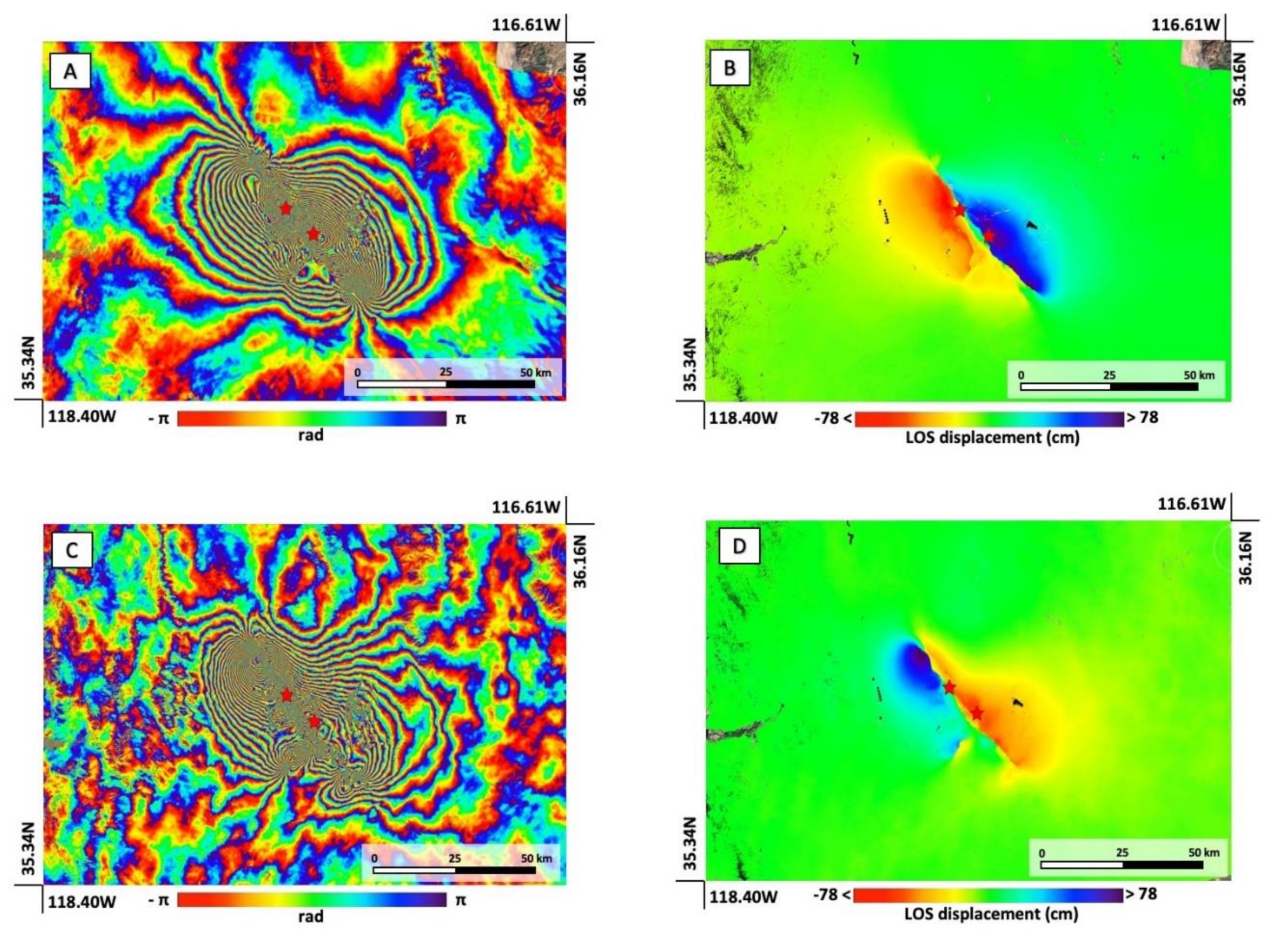
In
Figure 4, we show the coseismic interferograms and related displacement maps for both earthquakes. In particular,
Figure 4A,B reports the S1 coseismic interferogram and the corresponding deformation map, obtained by processing S1 descending images (Track 61) spanning the time interval 4 July 2019–16 July 2019, respectively.
Figure 4C,D shows the S1 coseismic interferogram and the corresponding deformation map, obtained from S1 ascending images (Track 71) spanning the time interval 4 July 2019–10 July 2019, respectively. Note that in
Figure 4A,C, the 2π radians variation corresponds to a displacement of about 2.8 cm for Sentinel-1, while in
Figure 4B,D, the red color corresponds to a sensor-target range increase and the blue one to a sensor-target range decrease. These conventions are valid for all of the following figures and are not replicated for brevity.
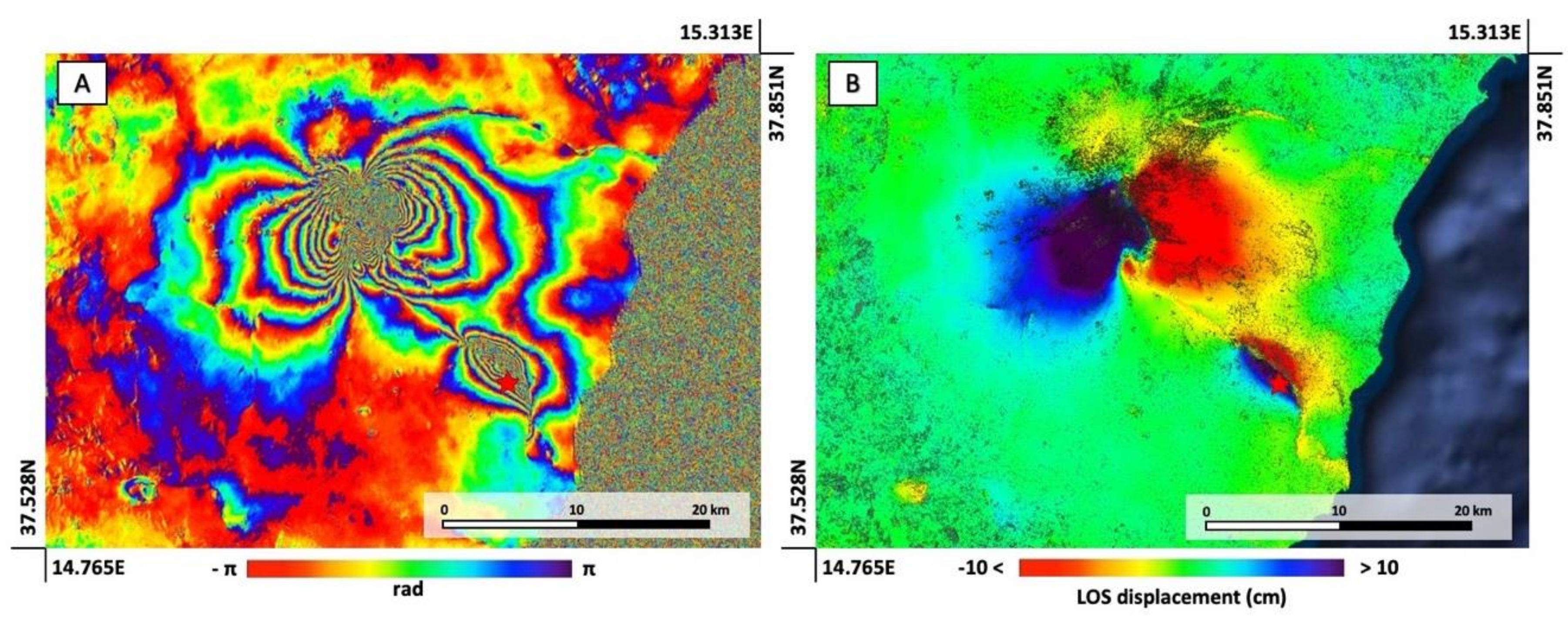
3.2. Earthquakes and Volcanic Eruptions
The seismic crisis that occurred between 22 and 28 December 2018, which was characterized by earthquakes between M
w 1.0 and 4.8, was propagated towards the south east sector of Mount Etna volcano (Italy). The strongest earthquake, which occurred along the Fiandaca Fault on 26 December 2018 with a M
w 4.8 and at a depth of 0.3 km, caused extensive damage to the surroundings in the town of Fleri (Catania). The main characteristics of this earthquake are detailed in [
37]. Moreover, the seismic swarm preceded, accompanied, and followed the Mt. Etna eruptive activity that took place on 24–27 December 2018. In
Figure 5, we show the S1 coseismic interferogram and related displacement map computed from ascending orbit (Track 44) images acquired on 22 and 28 December 2018.
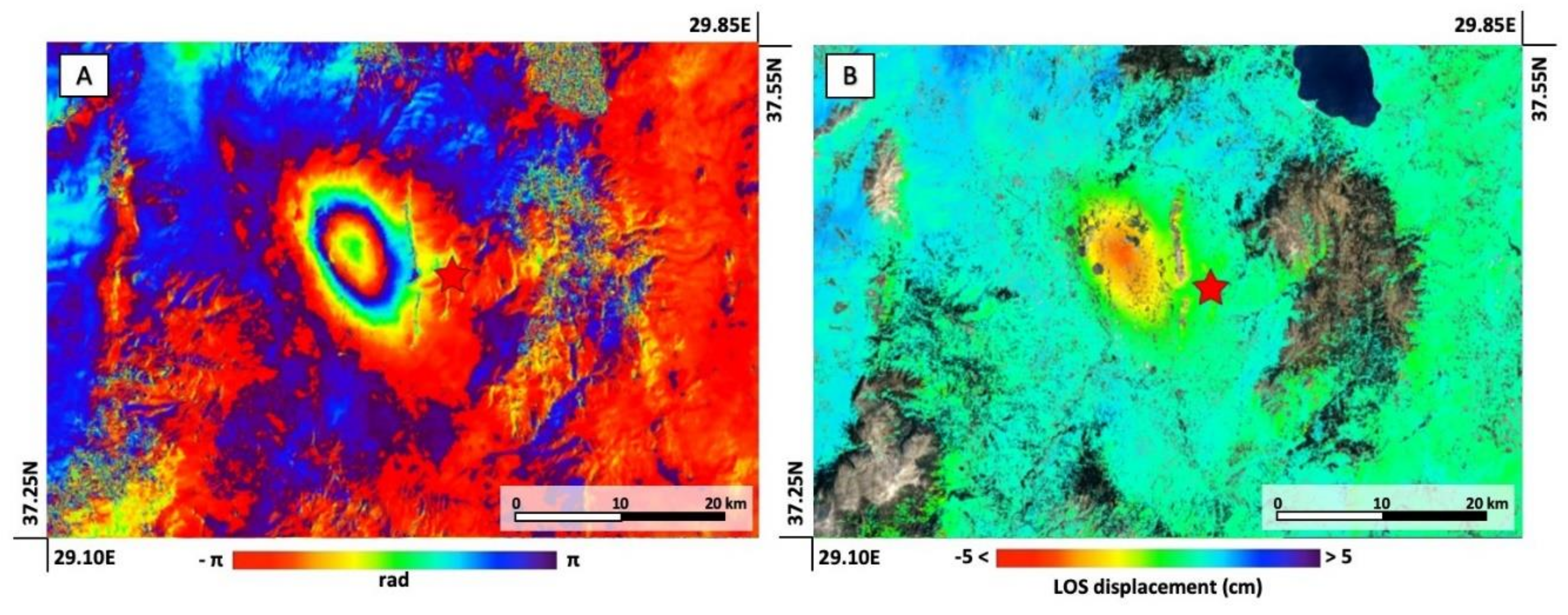
3.3. Earthquakes of a Small Magnitude
On 20 March 2019, a 5.7 M
w earthquake occurred a few kilometers away from the town of Acipayam, in Southwestern Turkey, at a depth of 8 km. This moderately strong earthquake was followed by ≈30 aftershocks, with the strongest measuring M
w 4.8. The focal mechanism from the USGS indicates that this event occurred along an approximately NW–SE trending fault with a predominantly normal mechanism. In
Figure 6, we present the coseismic interferogram and related deformation map obtained from S1 images acquired along descending orbits (Track 138) spanning the time interval 17 March 2019–23 March 2019 [
44].
3.4. Earthquakes That Occurred in the Same Area, but in Different Periods
In this subsection, we present two examples of multiple earthquakes hitting the same area in different periods.
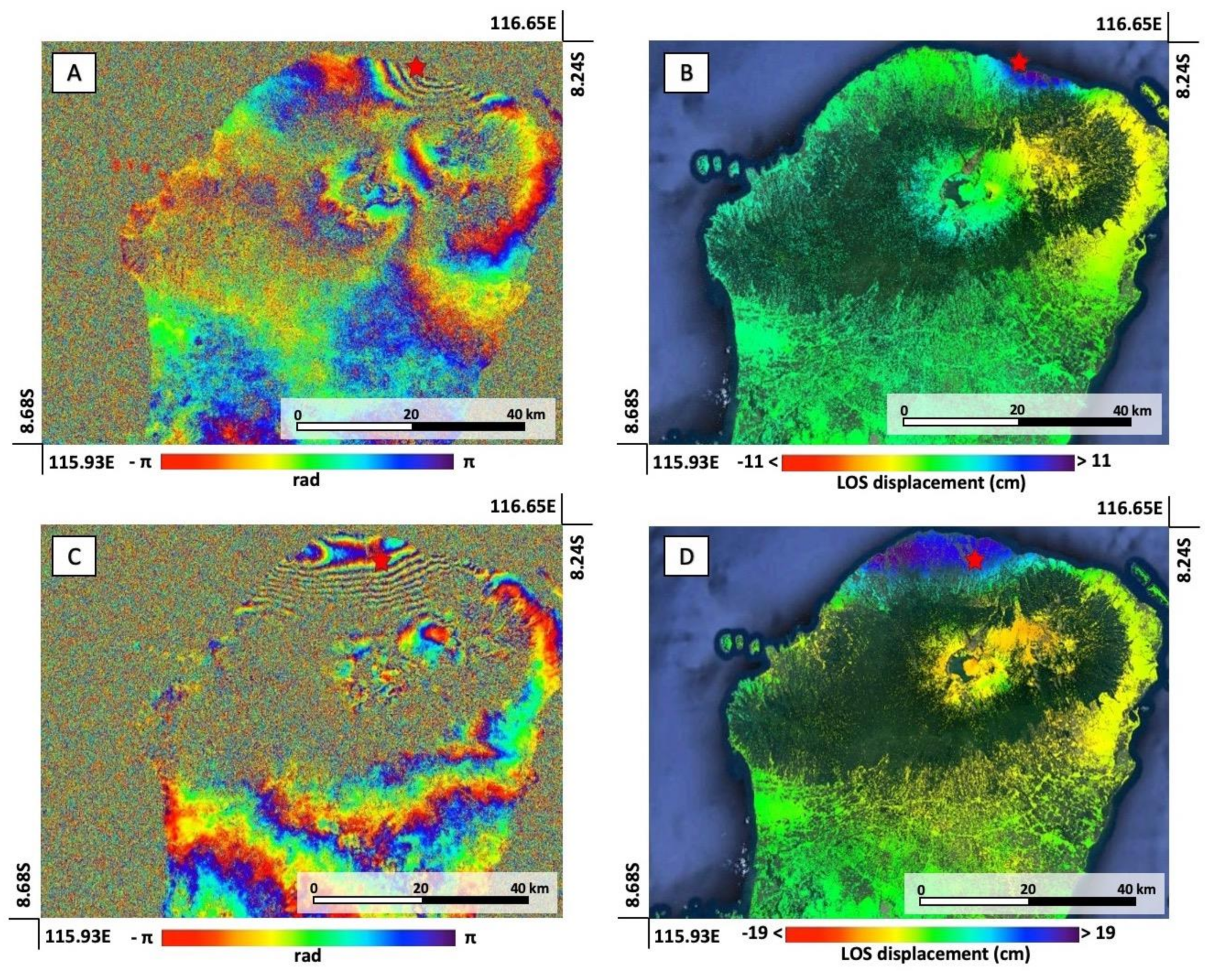
The first case is relevant to the seismic sequence that struck Lombok Island (Lesser Sonda Islands, Indonesia) between July 27 and August 25 2018, with 10 earthquakes with a significant magnitude (>5.5). The first earthquake occurred on 28 July, with a M
w 6.4 and a depth of 14 km; then, on 5 August, two earthquakes with a M
w 6.9 and 5.5 and depths of 34 and 31 km, respectively, hit the island. Subsequently, on 9 August, a new event occurred (M
w 5.9, depth of 15 km) and on 19 August, the island faced a seismic sequence of five earthquakes with M
w 6.3, 6.9, 5.6, 5.8, and 5.5 and depths from 10 to 21 km. Finally, the last earthquake occurred on 25 August, with M
w 5.5 and a depth of 11.6 km. The earthquake sequence in the north of Lombok was mainly due to back-arc thrust activity, as extensively described in [
45].
All of these earthquakes happened in a very short time period (less than one month) and the related epicenters were located very close to each other. The implemented DInSAR processing did not duplicate the processing jobs for new events occurring in this area, already struck by a previous earthquake, thus minimizing the time generation of new interferograms and related displacement maps.
As examples, we present the DInSAR results relevant to the 28 July and 5 August seismic events. In particular, in
Figure 7A,B, we show the S1 coseismic interferogram and related displacement map relevant to the 28 July earthquake, respectively. They were retrieved by using S1 ascending images (Track 32) covering the l8 July 2018–30 July 2018 interval.
Figure 7C,D shows the S1 coseismic interferogram and corresponding deformation map, relevant to the 5 August earthquake, obtained from S1 ascending images (Track 32) spanning the time interval 30 July 2018–5 August 2018, respectively.
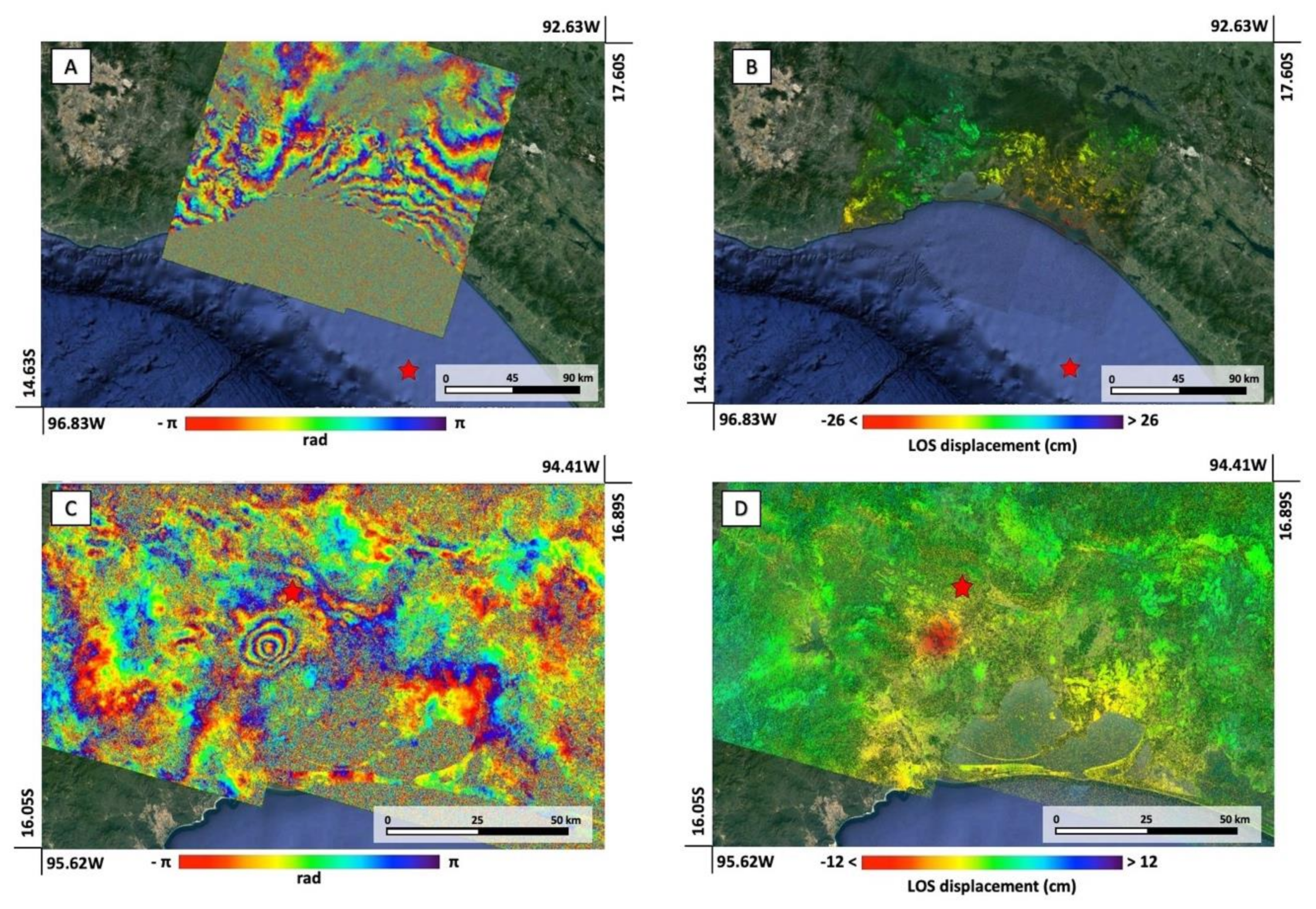
The second example is relevant to the seismic events that struck southern Mexico during September 2017.
In particular, the first earthquake occurred on 7 September off the southern coast of Mexico, near the state of Chiapas, approximately 100 km SSW of the town of Tres Picos (Chiapas), with a Mw 8.2 and a depth of 47.4 km; two weeks later, on 23 September, a second earthquake with a magnitude of Mw 6.1 and a depth of 10 km hit the area located about 24 km NE of San Jerónimo Ixtepec (Oxaca). Between these two events, other earthquakes occurred, such as the one (Mw 7.1, depth of 51 km) that struck the state of Puebla with an epicenter located south of the city of Puebla. For the sake of completeness, we point out that a few months later, on 12 February 2018, a new large earthquake hit San Pedro Jicayán (Oaxaca), with Mw 7.2 and a 22 km depth (see the next subsection).
The focal mechanism for the earthquake of M
w 8.2 shows that a slip occurred on either a fault dipping very shallowly towards the southwest, or on a steeply dipping fault striking NW–SE [
10]. The earthquake of M
w 6.1 shows a normal faulting mechanism solution [
10].
All of these earthquakes happened in a very short time period (less than a month) and the related epicenters were located not too far from each other if compared to the S1 swath width. As for the Lombok Island example, the implemented DInSAR processing did not duplicate the processing jobs (avoiding the start of useless additional runs of the procedure), thus optimizing the use of the available computing resources. As examples, we present the DInSAR results relevant to the 7 and 23 September seismic events. In particular, in
Figure 8A,B, we show the S1 coseismic interferogram and related displacement map relevant to the 7 September, respectively. They were retrieved by using S1 descending images (Track 172) spanning the 7 September 2017–13 September 2017 interval.
Figure 7C,D shows the S1 coseismic interferogram and corresponding deformation map, relevant to the 23 September earthquake, obtained from S1 descending images (Track 172) spanning the time interval 19 September 2017–25 September 2017, respectively.
3.5. Significant Seismic Events with Large Displacements
In this subsection, we present two examples of earthquakes that induced large ground displacements.
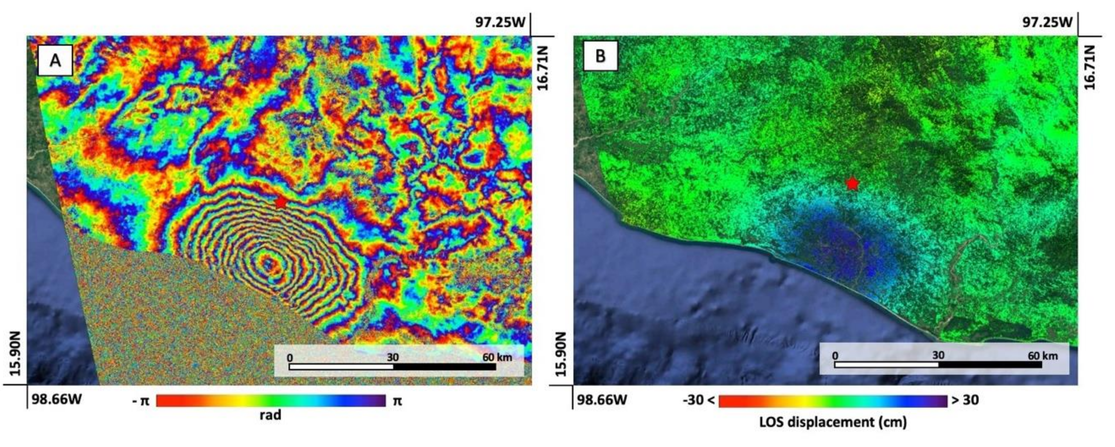
The first case is the M
w 7.2 seismic event that hit the state of Oxaca (Mexico) on 12 February 2018. It was characterized by an epicenter location close to the city of San Pedro Jicayán and a depth of 22 km. In
Figure 9, we report the S1 coseismic interferogram (
Figure 9A) and related displacement map (
Figure 9B) retrieved from ascending orbit (Track 5) images spanning 5 February 2018–17 February 2018. This earthquake occurred as a result of shallow thrust faulting on or near the plate boundary between the Cocos and North America plates, as described in [
10].
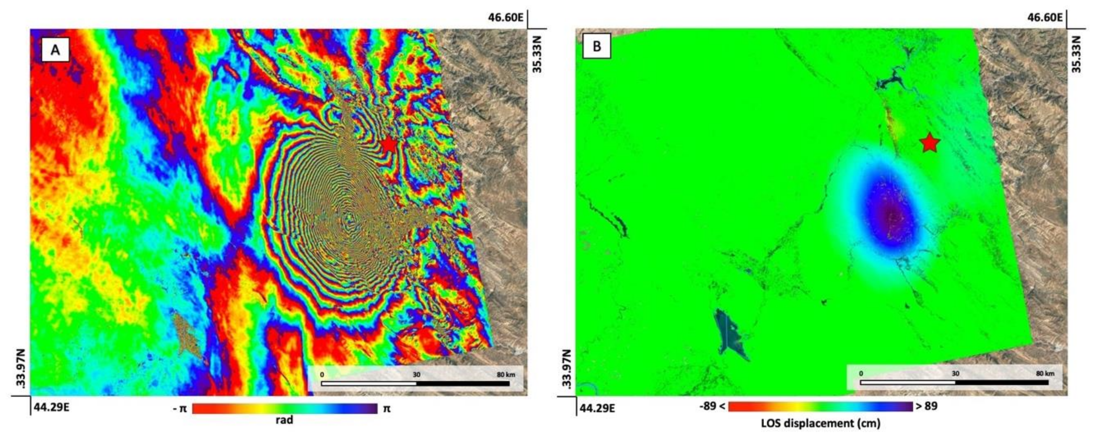
The second case regards the Halabjah earthquake (Iraq) that struck the Iran–Iraq border in northwest Iran (220 km northeast of Baghdad, Iraq), on 12 November 2017. This M
w 7.3 event had a 19 km depth, and was the result of oblique-thrust faulting at a mid-crustal depth (≈25 km). The preliminary focal mechanism solutions for the event indicate that rupture occurred on a fault dipping shallowly to the east–northeast, or on a conjugate fault dipping steeply to the southwest [
46].
In
Figure 10, we show the S1 coseismic interferogram (
Figure 10A) and related displacement map (
Figure 10B) retrieved from ascending orbit (Track 72) images spanning 11 November 2017–17 November 2017.
We highlight that both cases are representative of strong earthquakes;
Figure 9A and
Figure 10A reveal the presence of very high fringe rates that correspond to very large deformation signals (
Figure 9B and
Figure 10B) on the ground (more than 30 and 90 cm, respectively).
3.6. Earthquakes Located in the Sea
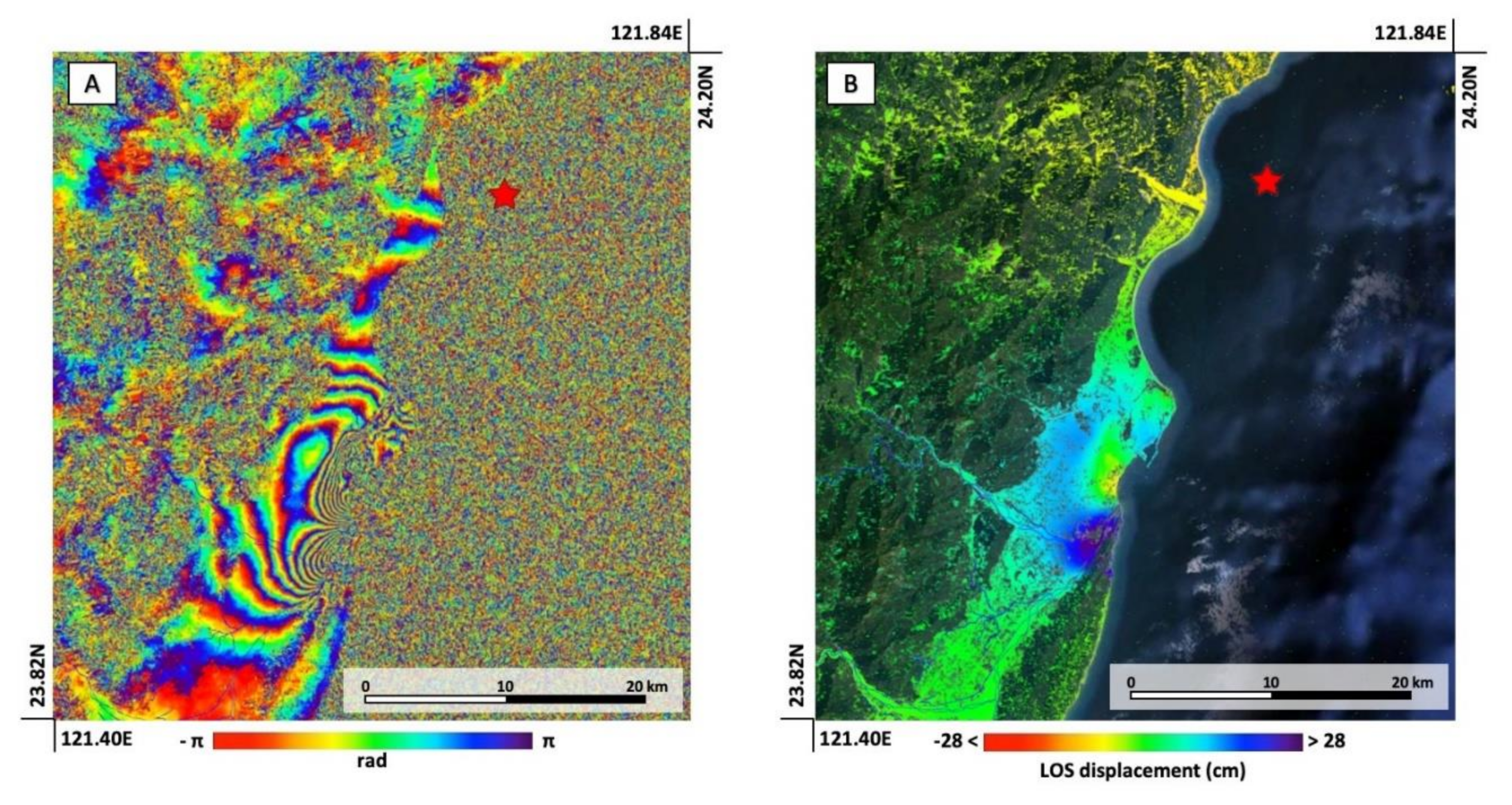
On February 2018, an earthquake swarm struck northeastern and eastern Taiwan. The first event occurred on 4 February 2018 about 22 km NNE of the Hualien city (Taiwan) with a M
w 6.1 and a 12 km depth; the epicenter of this earthquake was located offshore. It was followed by several earthquakes with a similar magnitude, all occurring within a very short time span (a couple of days), culminating with a M
w 6.4 earthquake that struck eastern Taiwan on 6 February. This earthquake occurred in the northern extension of the Coast Range, which is the junction of the collision and subduction boundaries between the Eurasian plate and the Philippine Sea plate. The focal mechanism derived from teleseismic data shows that the coseismic fault of the 2018 Hualien event had a strike angle of 209° and dipped to the west with a high dip angle of 73° and rake angle of 22° [
47,
48].
In
Figure 11, we show the DInSAR results relevant to the 4 February seismic event. In particular, in
Figure 11A, we show the S1 coseismic interferogram, and in
Figure 11B, the related displacement map; both were retrieved from ascending orbit (Track 69) images acquired on 3 and 9 February 2018.
4. Discussion
We presented an unsupervised tool for the automatic generation of coseismic DInSAR products at a global scale by means of Sentinel-1 data. Although conceived for Sentinel-1 data, the tool we implemented is independent of the SAR acquisitions used. The only dependency is on the catalog interface that requires the implementation of appropriate wrappers, while the processing module (Block D
Figure 1) can be substituted without impacting the general workflow. Tuning and refinement of the proposed thresholds might also be necessary for different locations and seismic catalogs.
The Cloud Computing services of the AWS infrastructure were used, not only for their processing capacity, but also for the online availability of the S1 archive. Despite the specific implementation in AWS, the developed tool relies on common IT methods and protocols, thus implying its portability to different computing platforms, such as the European Commission DIAS [
23], where satellite data (mainly Copernicus) and processing facilities are also co-located to reduce the transfer time during the processing.
The main results of the implemented tool consist of pre-, co-, and post-seismic (up to 36 days after the event) displacement maps, along the satellite LOS, relevant to every identified earthquake. A set of coseismic interferograms and displacement maps, related to different scenarios and case studies, were presented to demonstrate the effectiveness of the implemented tool.
Since the Sentinel-1 system is highly reliable in terms of the operational capacity and since the exploited processing chain has been well-tested with a significantly large number of cases [
18], the processing success rate is close to 100%. The main issues that can hamper the generation of DInSAR products are linked to the actual data availability for specific areas of the Earth. In particular, when dealing with small islands, the system can detect an earthquake close enough to the land to trigger the processing. Then, it could be that the SAR data searching window is large enough to retrieve Sentinel-1 images, which do not actually cover the island. This particular behavior implies that the DInSAR processing starts without generating any usable products. To manage such an issue, a check of the coherence histogram is performed to avoid the publication of completely noisy results.
Another issue is due to possible miscomputation of the residual azimuth shift when applying the ESD procedure. Indeed, the ESD works fine when a minimum coherence is guaranteed on the Sentinel-1 burst overlap areas. The main cause of a lack of coherence is the presence of water in the imaged scene, as is likely to occur in small island cases.
While the processing issues can, to a certain extent, be constrained, the usual sources of error in DInSAR products are always present. The main ones are represented by atmospheric disturbances and phase unwrapping issues. Detecting such errors in an automatic way for single interferograms is practically impossible. For instance, several large spatial scale components of atmospheric disturbances can be removed by resorting to external information (e.g., weather models [
49]), while small-scale turbulences are extremely difficult to filter out. Accordingly, to permit the user to mitigate such sources of error, the proposed tool generates multiple coseismic interferograms by exploiting different data pairs. This data redundancy allows discrimination of the phase components correlated in time (typically due to permanent surface deformation) from those that are not time coherent (such as the atmospheric disturbances). The same approach can also be useful for identifying possible phase-unwrapping errors, as well as highlighting post-seismic displacement effects.
The existing processing chain can be further improved by applying additional filters to the interferograms, such as the aforementioned ones devoted to the reduction of atmospheric disturbances by exploiting external weather models [
49]. Moreover, the possibility to introduce more sophisticated spatial filters to increase the SNR of the interferometric phase is also envisaged [
50]. We further remark that the developed tool can also be extended with additional post-processing steps for generating analytical source models (upon general elastic and homogeneous half-space conditions [
51]) from the retrieved DInSAR displacement maps. This could permit having an immediate, although rough, idea of the involved seismic source, in order to better understand the fault mechanism that generated the earthquake.
Furthermore, another improvement can be achieved by disposing of an a priori estimation of the area affected by the deformation, which can be retrieved by applying forward models based on the earthquake characteristics and then projecting the expected deformation along the satellite LOS. This a priori information can be extremely useful for driving the SAR data selection, the reference point identification, and the phase unwrapping step for earthquakes that present high fringe rate patterns.
The global generation of coseismic maps from satellite DInSAR data is presently a hot research topic, as testified by other works providing tools or services similar to the one herein presented. Among them, it is worth mentioning LiCSAR [
26], which is maintained by the UK COMET consortium, and systematically provides interferograms for all of the Earth’s seismic regions, regardless of the occurrence of an earthquake. The Advanced Rapid Imaging and Analysis (ARIA) system [
25], handled by the Jet Propulsion Laboratory (JPL), which is activated upon the request of ARIA members, is generally focused on US regions, and provides not only DInSAR maps, but also several other products related to natural hazards. Similarly, the SARVIEWS system [
27], managed by the Alaska Satellite Facility (ASF), provides DInSAR, as well as change detection and other types of maps; it acts worldwide and is generally triggered by large seismic events. In this context, the service we propose generates DInSAR products for seismic events with a magnitude (M
w) larger than 5.5 at a global scale, while particular focus is placed on shallow and small magnitude (larger than M
w 4.0) events in Italy. Our service is one of those provided within the EPOS Research Infrastructure framework.
Finally, an implementation of the proposed tool is currently experimentally running to serve the Italian Department of Civil Protection (DPC) in the framework of the monitoring activities of the Institute for the Electromagnetic Sensing of the Environment (IREA). Generated DInSAR products are used to map the extent of the area affected by surface deformation to help post-earthquake crisis management. DInSAR data can also be used to relocate earthquakes after inverting the deformation measurements for retrieving the seismic source. Moreover, from the available displacement maps, it is possible to compute accurate source models that can also permit estimations of stress accumulation and possible future ruptures.
5. Conclusions
In this work, we presented an automatic and unsupervised tool for the systematic generation of S1 DInSAR coseismic products, represented by displacement maps, interferograms, and spatial coherence. In particular, our procedure first retrieves the location, depth, and magnitude of each seismic event from interoperable online earthquake catalogs (e.g., USGS and INGV) and then automatically triggers the downloading of S1 data and processing over the area affected by the earthquake if the selected seismic event is identified as significant with respect to a set of selected thresholds. Moreover, we presented examples relevant to several earthquakes with different characteristics in terms of the magnitude, epicenter location, depth, and space–time separation, which occurred globally in recent years, proving the effectiveness of the implemented procedure.
The presented results show that the developed automatic and unsupervised tool:
Allows the creation of a global database of DInSAR S1 coseismic products by exploiting the S1 archive since 2015 (a date that corresponds to the primary availability of Sentinel-1 images). These results will be progressively made openly available through the EPOS Research Infrastructure, which represents a key reference for the wide scientific community of Solid Earth in Europe. This generated DInSAR earthquake database can boost the comprehension of Earth system dynamics in the seismic zones around the world. Indeed, the joint exploitation of huge data archives and computing resources will pave the way to a new approach to science, based on data-intensive exploration and analysis, which might lead to important advances in earthquake science;
Can provide key support to national and local civil protection authorities during seismic crises, given its capability to retrieve coseismic DInSAR products in a very short time. This further demonstrates the tool’s capability to be used in “real-life” operational scenarios.

 ,
, 


