Figure 1.
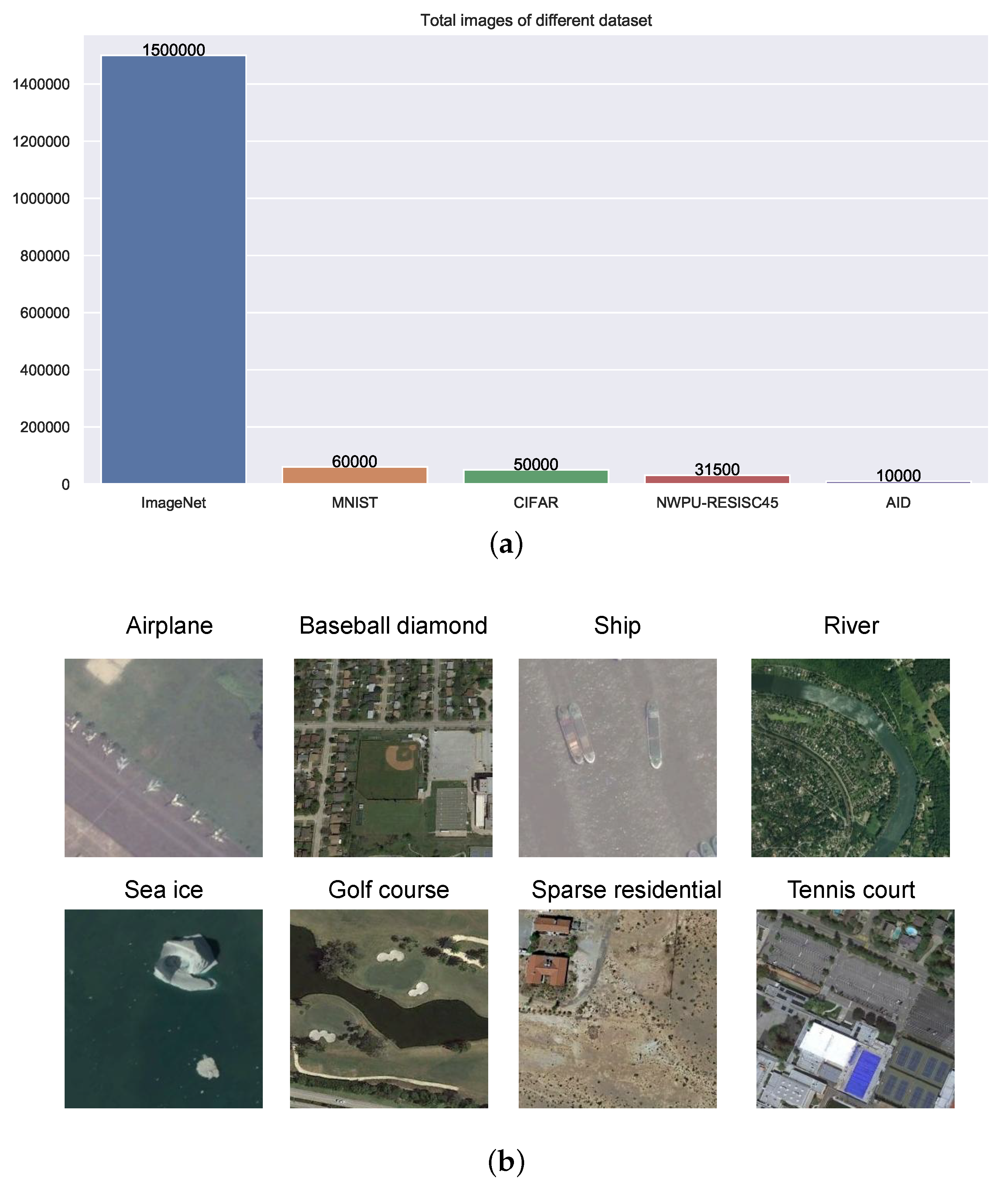
Two main problems exist: (a) Compared with datasets of natural images, the total numbers of images in remote sensing image datasets are much smaller. (b) Compared with natural images, it is difficult to find discriminative semantic features in remote sensing scene images because features containing semantic information may lie within a small area against a complex background.
Figure 1.
Two main problems exist: (a) Compared with datasets of natural images, the total numbers of images in remote sensing image datasets are much smaller. (b) Compared with natural images, it is difficult to find discriminative semantic features in remote sensing scene images because features containing semantic information may lie within a small area against a complex background.
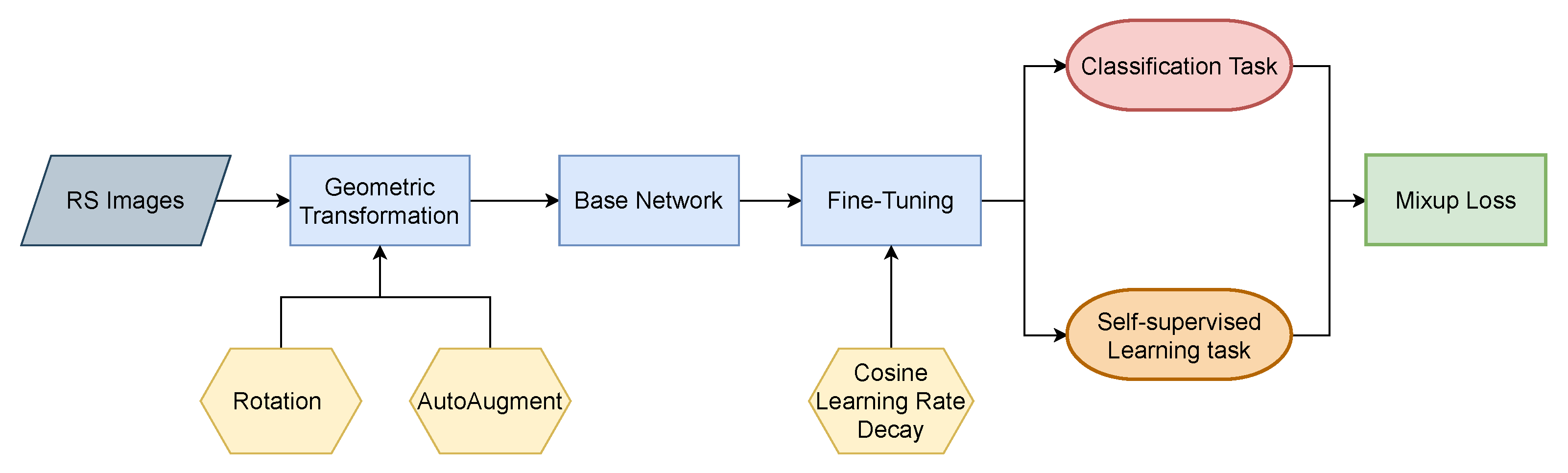
Figure 2.
Flowchart of the proposed framework.
Figure 2.
Flowchart of the proposed framework.
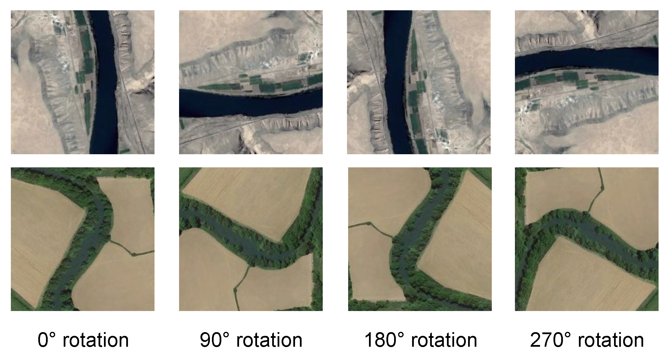
Figure 3.
Example images rotated by random multiples of 90 degrees (e.g., 0, 90, 180, or 270 degrees). The core intuition of self-supervised learning is that if the CNN model is not aware of the concepts of the objects depicted in the images, it cannot recognize the rotation that was applied to them.
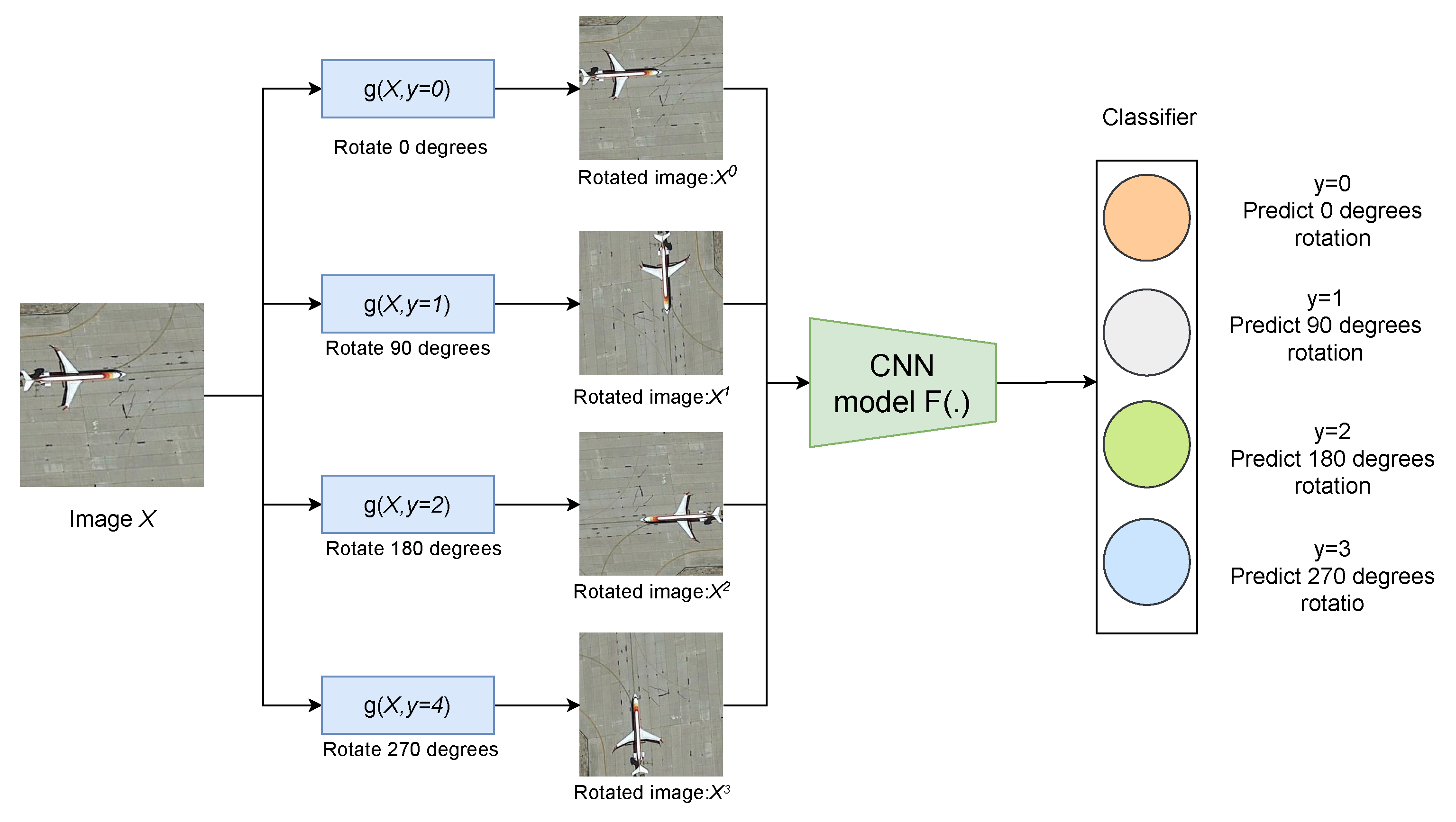
Figure 4.
Illustration of the self-supervised learning task that we propose for semantic feature learning. Given four possible geometric transformations, i.e., rotations by 0, 90, 180, and 270 degrees, we train a CNN model to recognize the rotation that has been applied to the image that it receives as input.
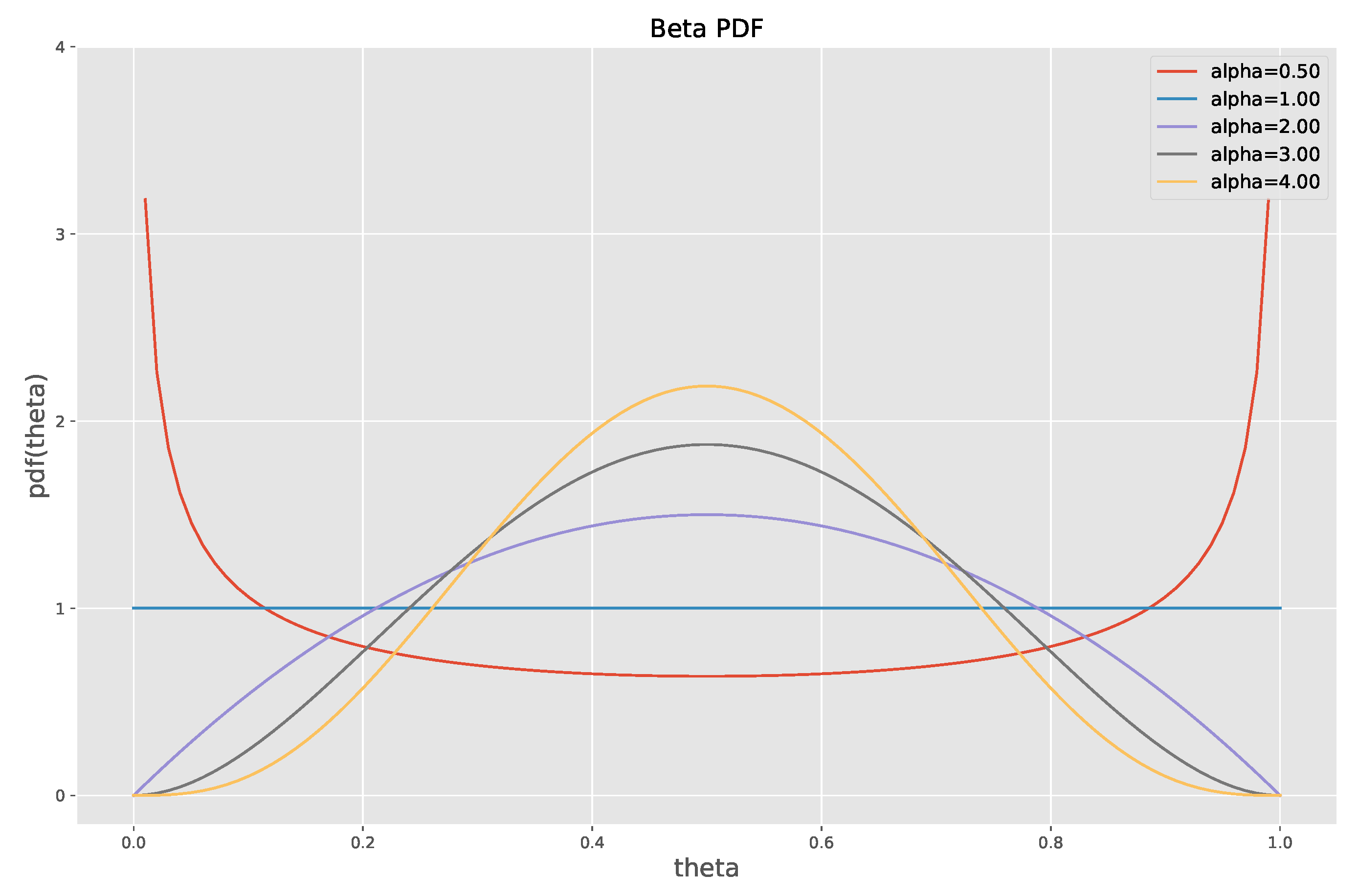
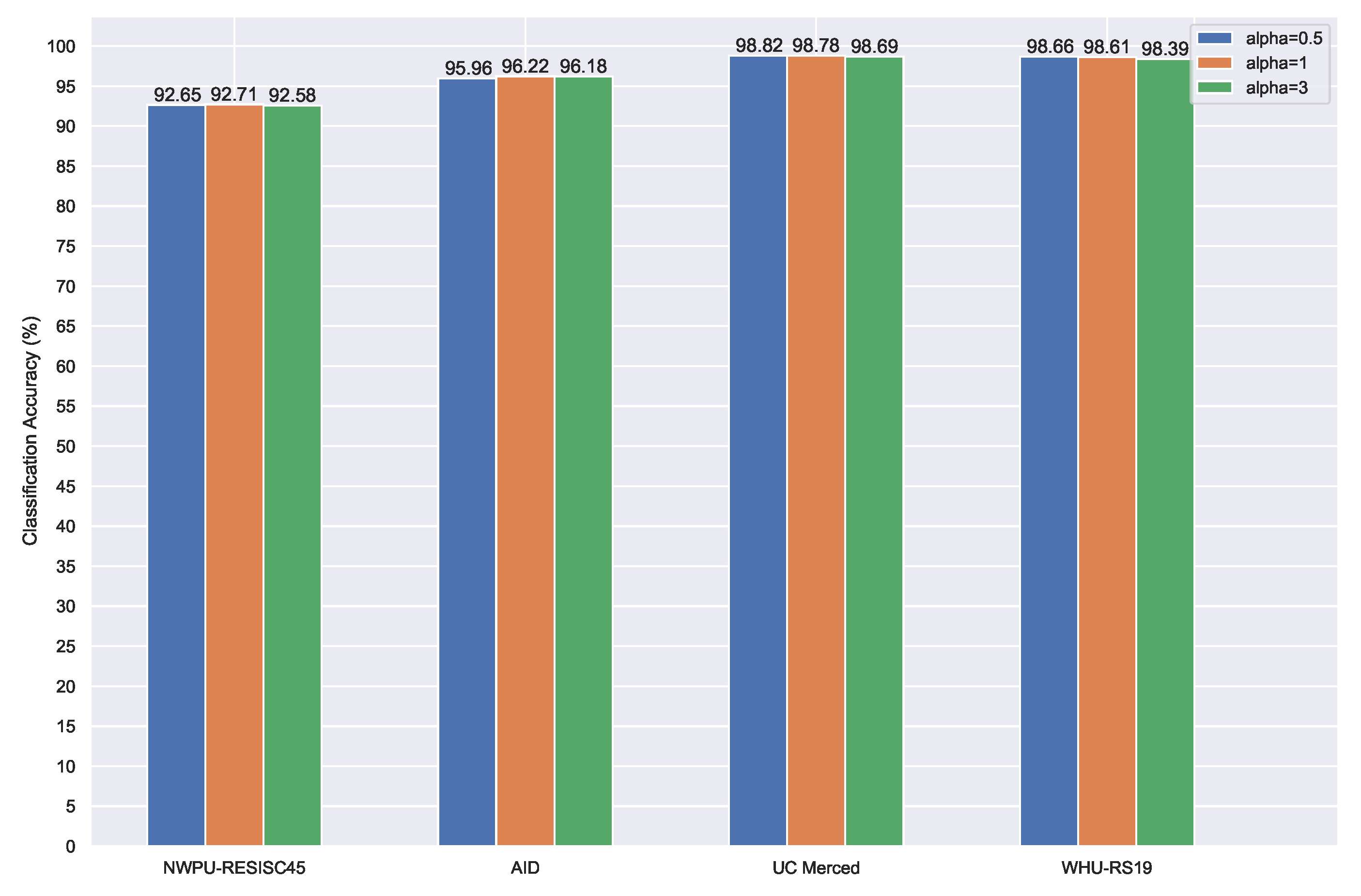
Figure 5.
The probability density functions for the beta distribution with different values of .
Figure 5.
The probability density functions for the beta distribution with different values of .
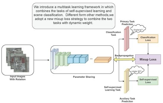
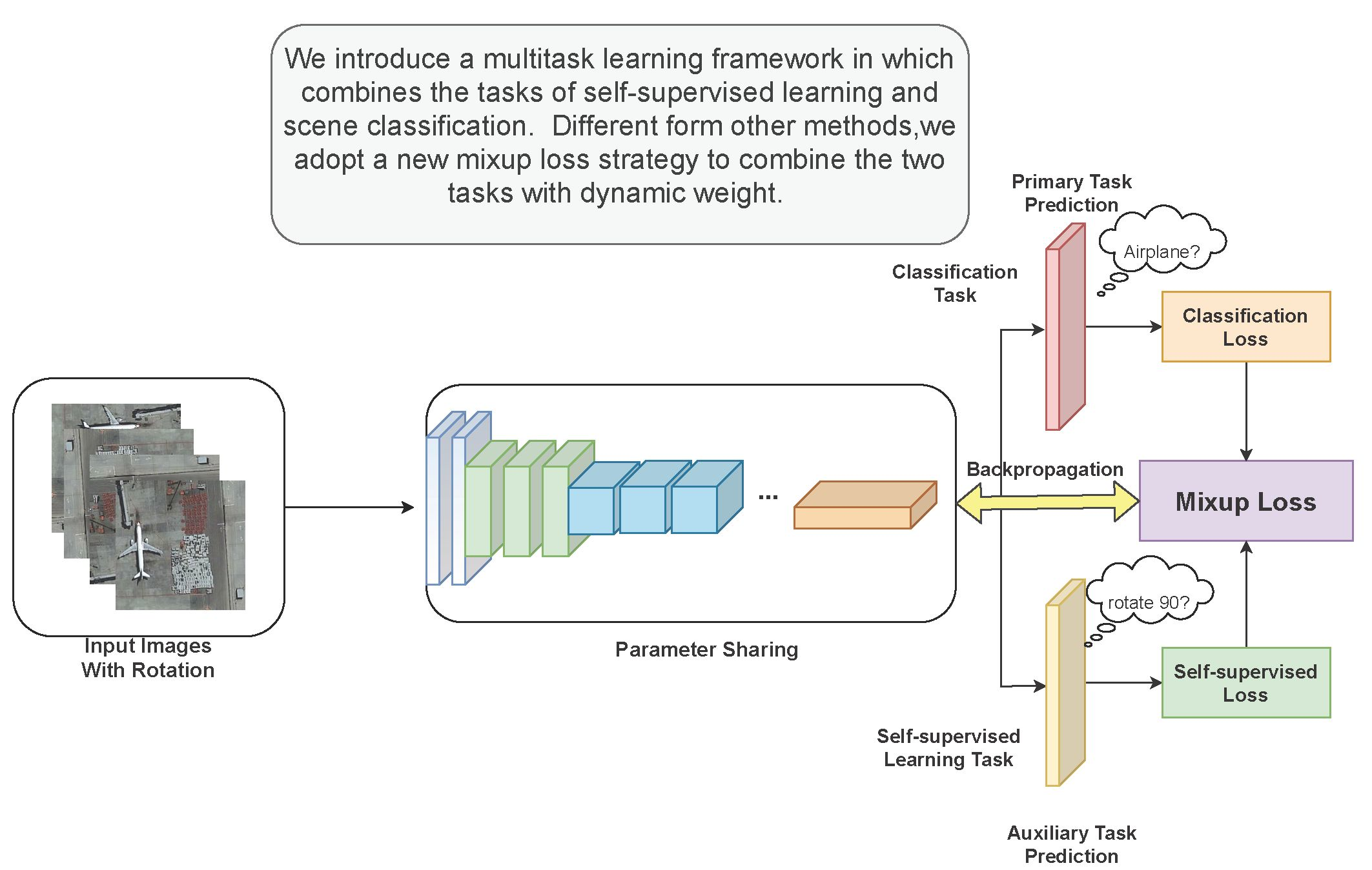
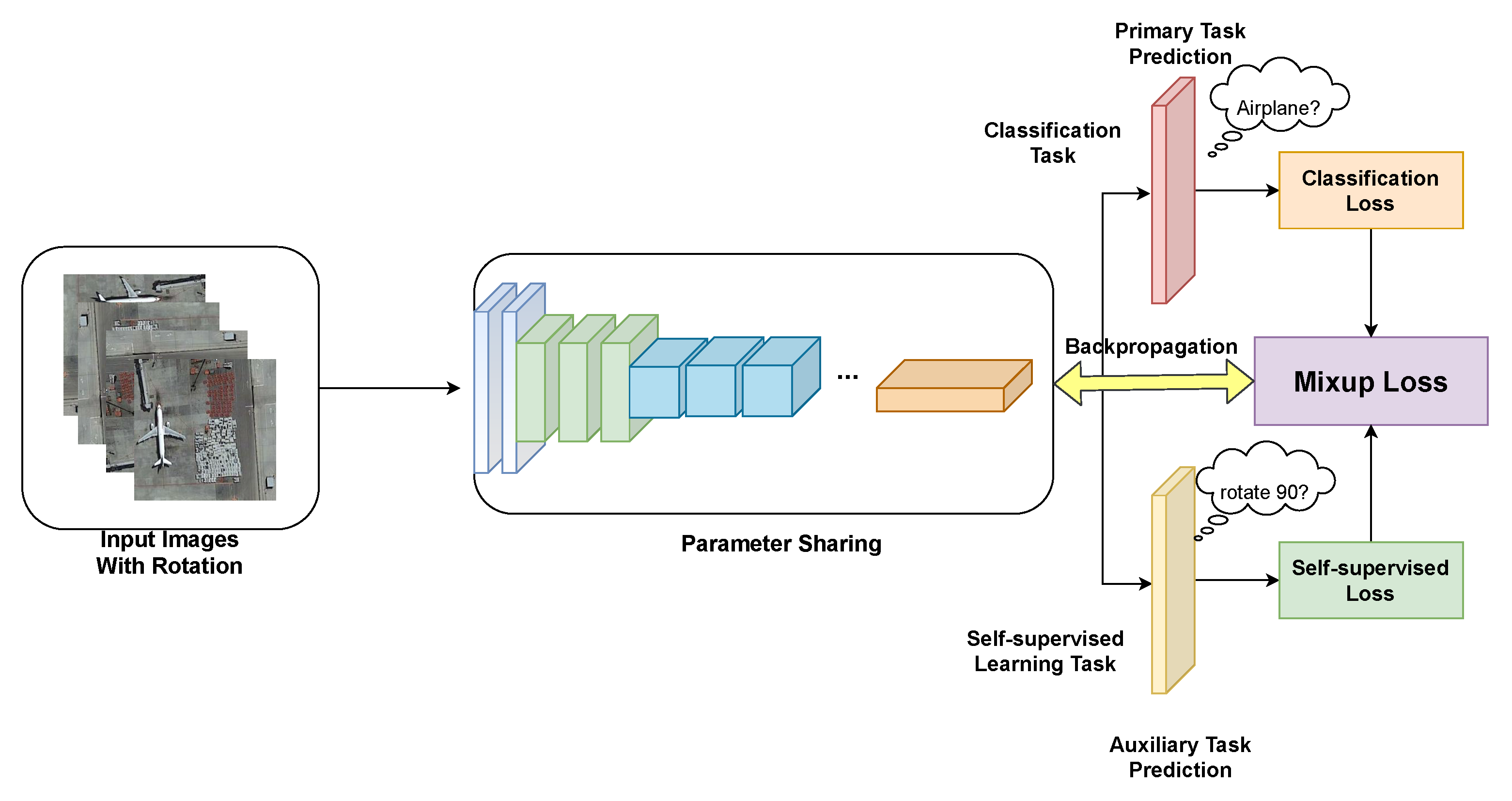
Figure 6.
Architecture of the proposed multitask learning (MTL) framework. Multiple input images are generated from a single image by rotating by 90, 180, and 270 degrees. The network is trained on two tasks. The main task is the classification task, of which the aim is to identify a determinate category for each remote sensing scene. The auxiliary task is a self-supervised learning task in which the aim is to obtain the rotation label. The two tasks are combined using the mixup loss strategy.
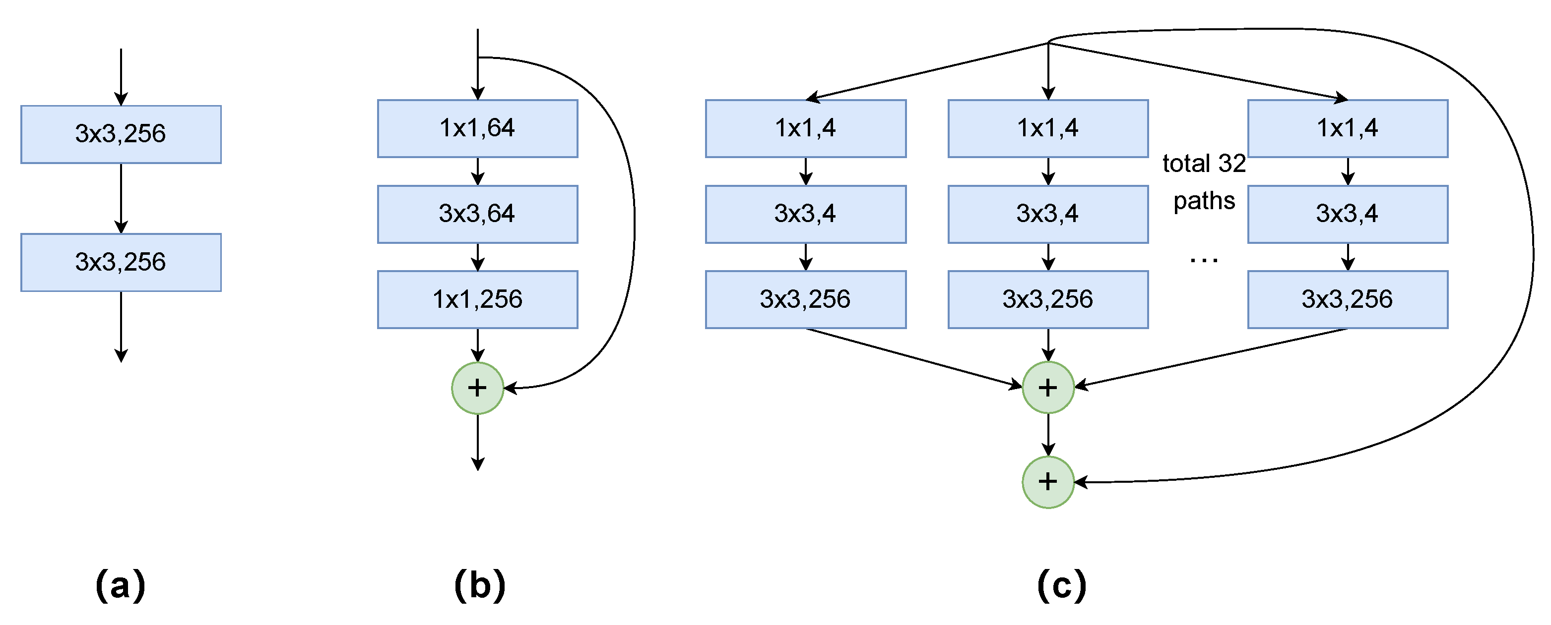
Figure 7.
Three different network building blocks: (a) A VGG block. (b) A ResNet block. (c) A ResNeXt block.
Figure 7.
Three different network building blocks: (a) A VGG block. (b) A ResNet block. (c) A ResNeXt block.
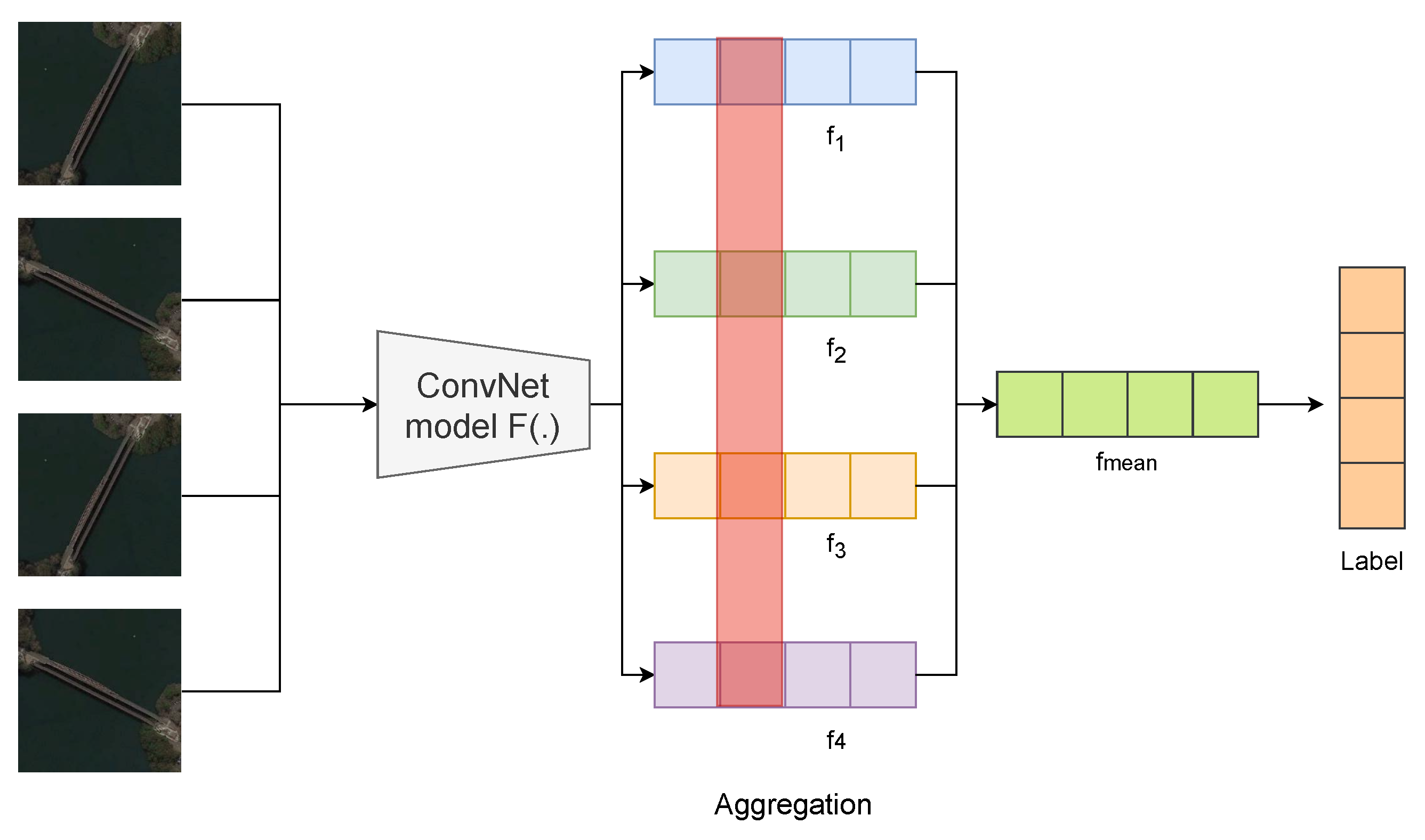
Figure 8.
In the test stage, is obtained by aggregating the four different feature descriptors , , , and . Then, is used for prediction.
Figure 8.
In the test stage, is obtained by aggregating the four different feature descriptors , , , and . Then, is used for prediction.
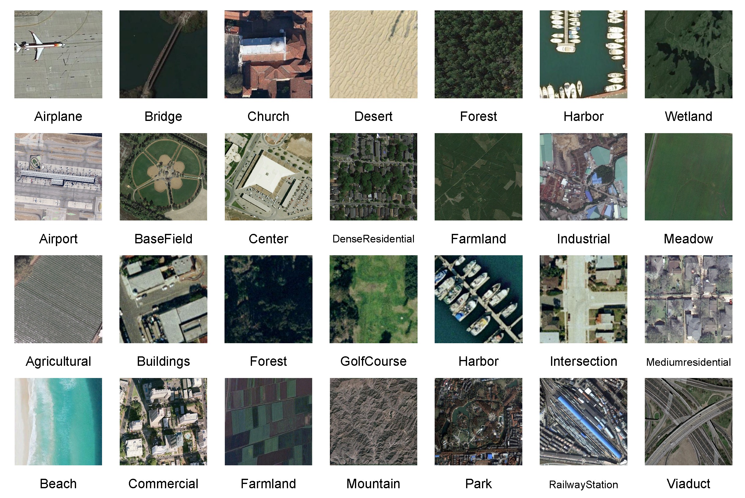
Figure 9.
Example images from the four remote sensing scene classification datasets. From the top row to the bottom row: NWPU-RESISC45, AID, UC Merced, and WHU-RS19.
Figure 9.
Example images from the four remote sensing scene classification datasets. From the top row to the bottom row: NWPU-RESISC45, AID, UC Merced, and WHU-RS19.
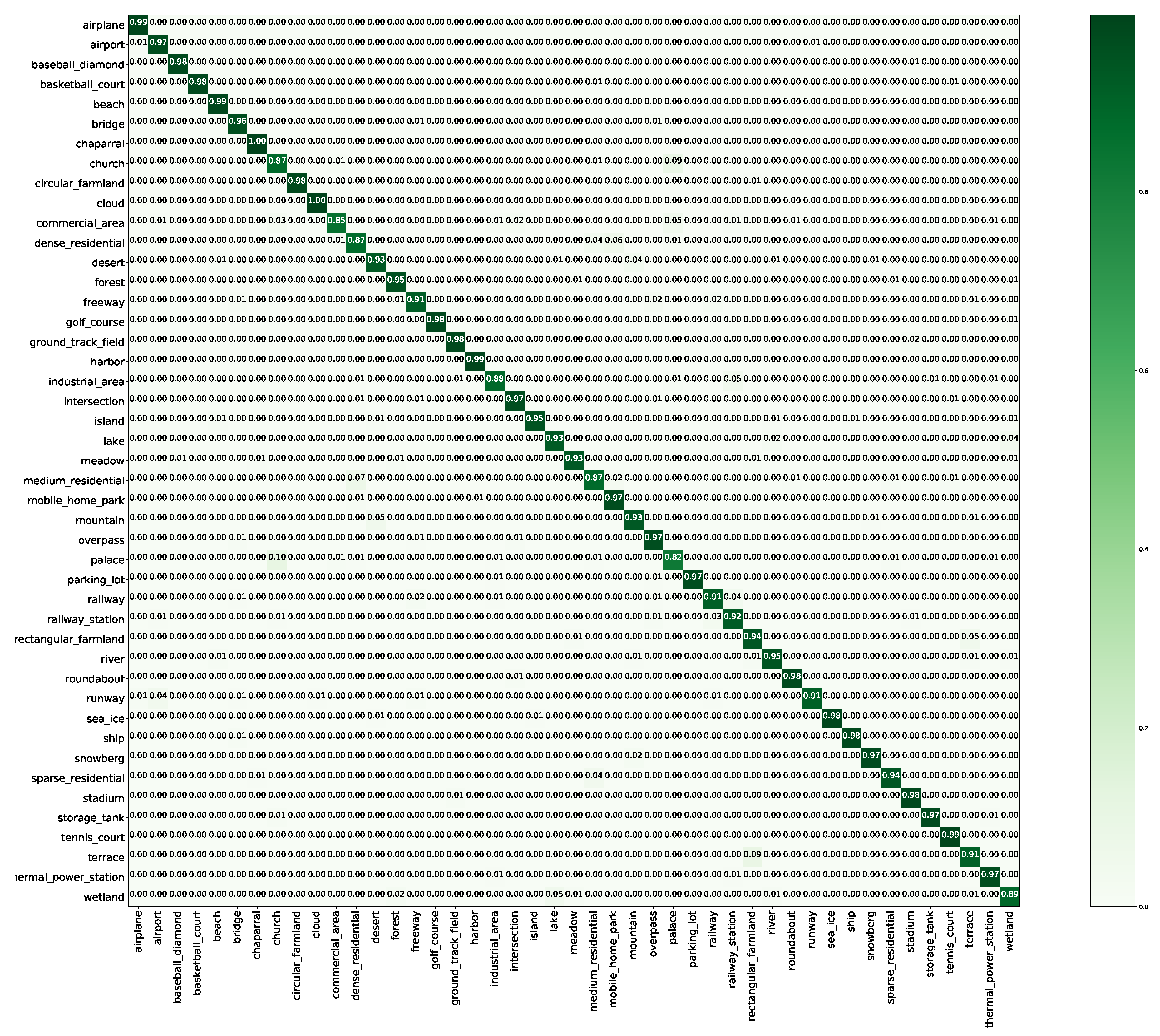
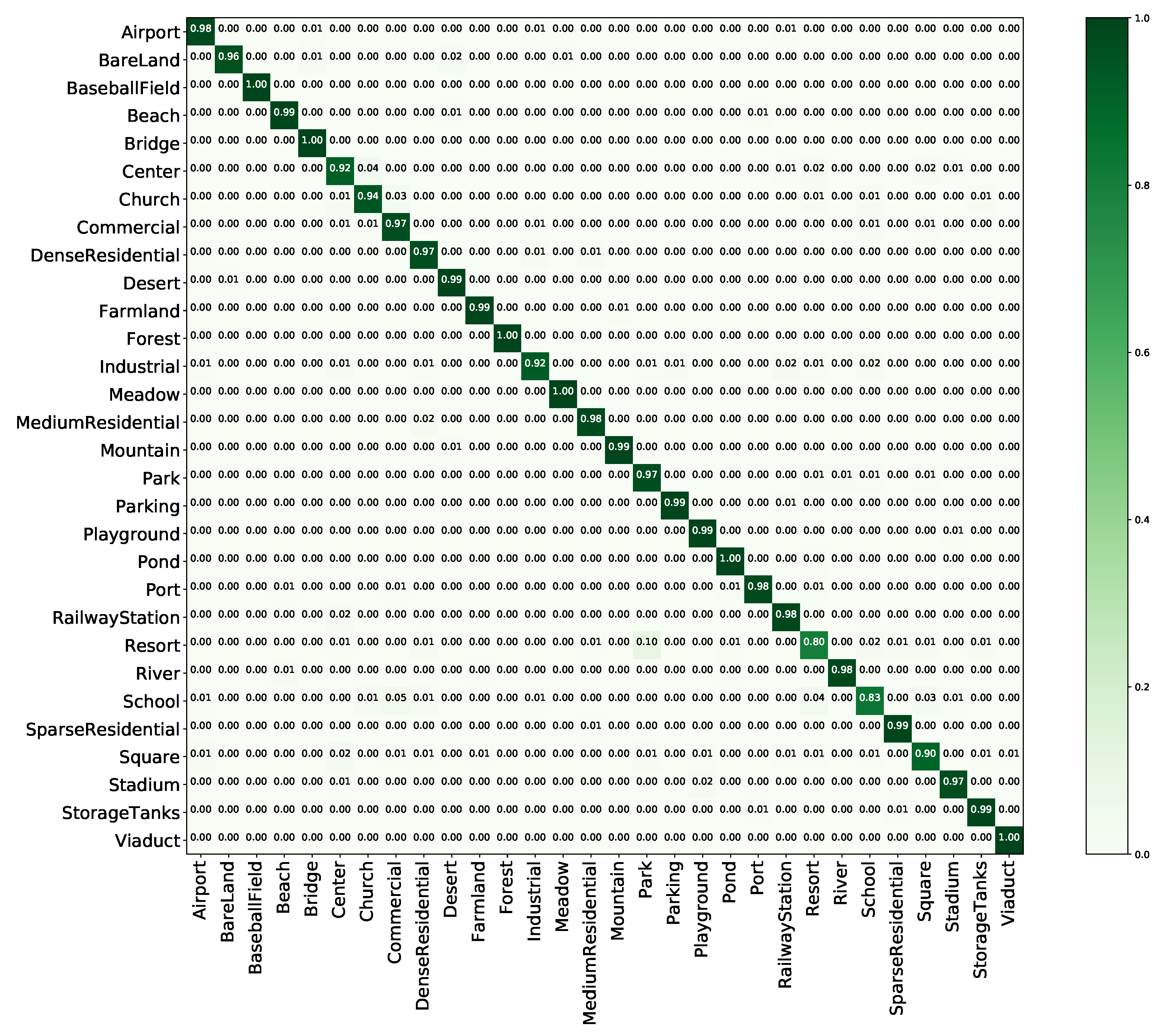
Figure 10.
Confusion matrix of the proposed method on the NWPU dataset with a training proportion of 20%.
Figure 10.
Confusion matrix of the proposed method on the NWPU dataset with a training proportion of 20%.
Figure 11.
Confusion matrix of the proposed method on AID with a training proportion of 50%.
Figure 11.
Confusion matrix of the proposed method on AID with a training proportion of 50%.
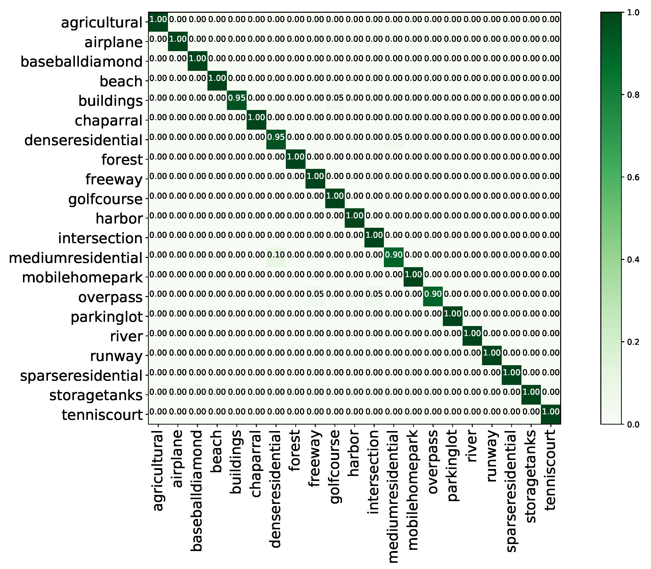
Figure 12.
Confusion matrix of the proposed method on the UC Merced land use dataset with a training proportion of 80%.
Figure 12.
Confusion matrix of the proposed method on the UC Merced land use dataset with a training proportion of 80%.
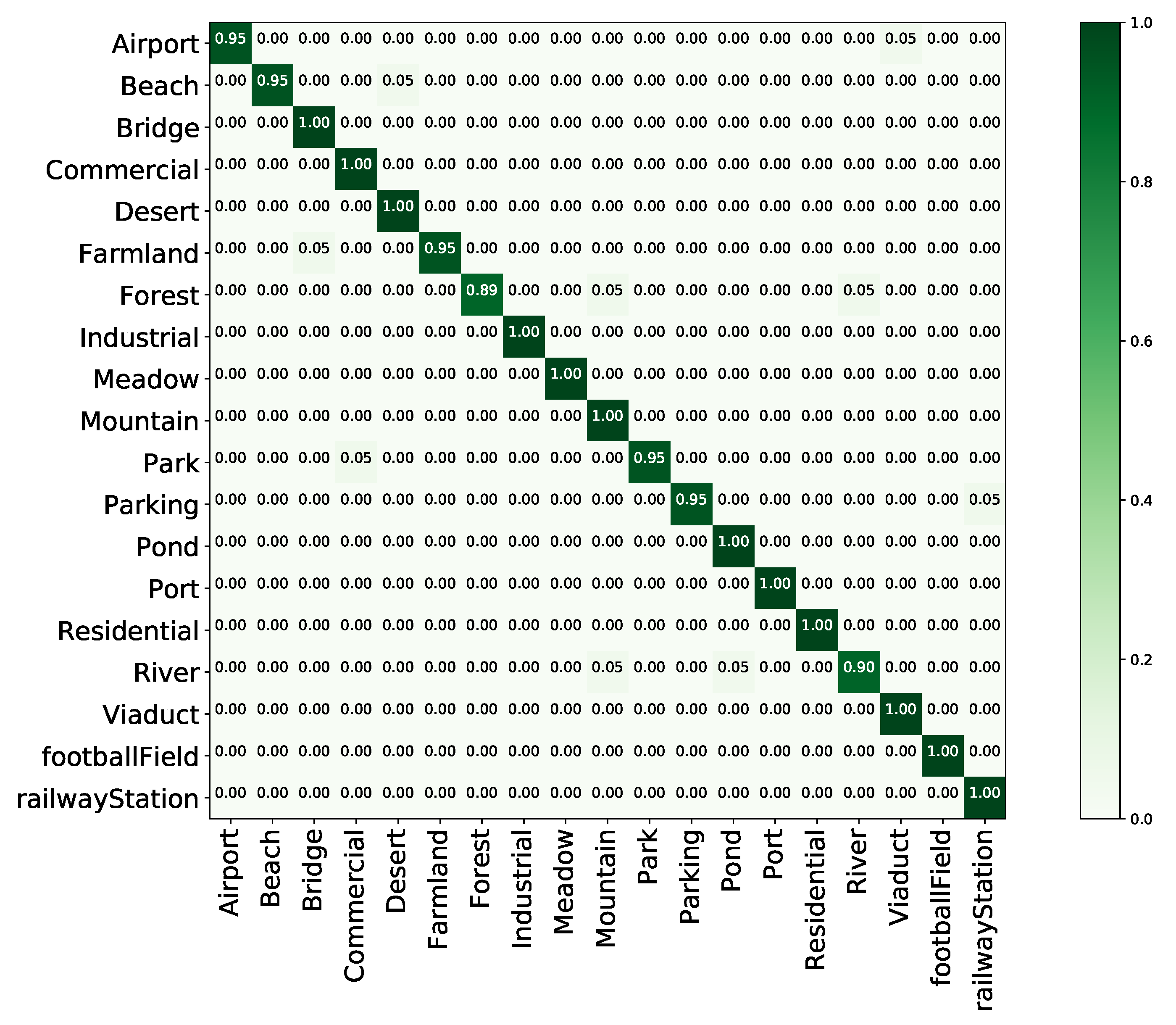
Figure 13.
Confusion matrix of the proposed method on the WHU-RS19 dataset with a training proportion of 60%.
Figure 13.
Confusion matrix of the proposed method on the WHU-RS19 dataset with a training proportion of 60%.
Figure 14.
Overall accuracy (%) of the proposed method with and without MTL on the four datasets.
Figure 14.
Overall accuracy (%) of the proposed method with and without MTL on the four datasets.
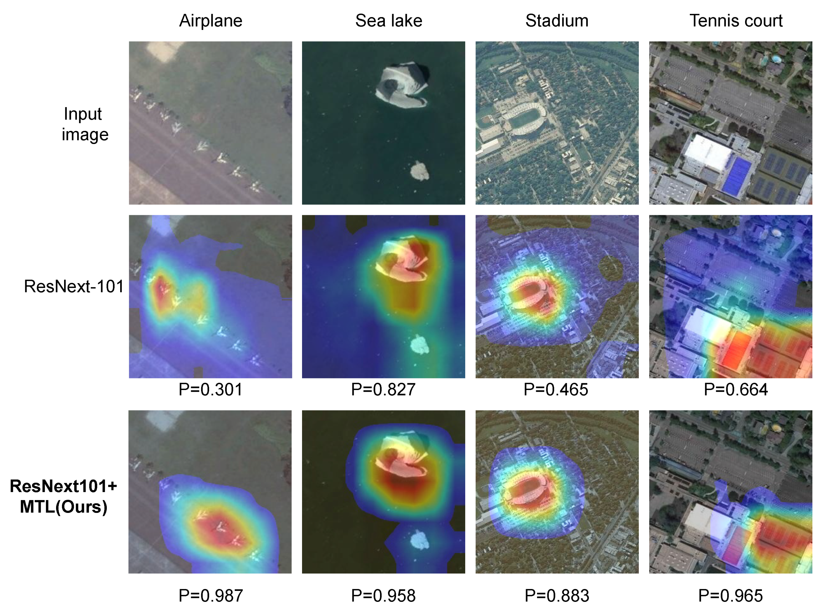
Figure 15.
Grad-CAM [
66] visualization results. We compare the visualization results obtained using an MTL-trained network (ResNeXt-101+MTL) with those of the corresponding baseline model (ResNeXt-101). The Grad-CAM visualization was calculated for the last convolutional outputs. The ground-truth labels are shown above each input image, and P denotes the softmax score of each network for the ground-truth class.
Table 1.
Comparison of the four different remote sensing scene datasets.
Table 1.
Comparison of the four different remote sensing scene datasets.
| Dataset | Images per Class | Scene Classes | Total |
|---|
| NWPU-RESISC45 | 700 | 45 | 31,500 |
| AID | 200–480 | 30 | 10,000 |
| UC Merced | 100 | 21 | 2100 |
| WHU-RS19 | 50 | 19 | 1005 |
Table 2.
Comparison of model performance with and without MTL. The bold results are obtained by our proposed method.
Table 2.
Comparison of model performance with and without MTL. The bold results are obtained by our proposed method.
| Method | NWPU (0.2) | AID (0.5) | UC Merced (0.8) | WHU-RS19 (0.6) |
|---|
| VGG-16 | | | | |
| VGG-16+MTL (ours) | | | | |
| ResNet-50 | | | | |
| ResNet-50+MTL (ours) | | | | |
| ResNet-101 | | | | |
| ResNet-101+MTL (ours) | | | | |
| ResNeXt-50 | | | | |
| ResNeXt-50+MTL (ours) | | | | |
| ResNeXt-101 | | | | |
| ResNeXt-101+MTL (ours) | | | | |
Table 3.
Comparisons of aggregation prediction and single-image prediction. The bold results are obtained by our proposed method.
Table 3.
Comparisons of aggregation prediction and single-image prediction. The bold results are obtained by our proposed method.
| Methods | Prediction Methods | Accuracy(%) |
|---|
| ResNext-50+MTL | single-image | |
| aggregation | |
| ResNext-101+MTL | single-image | |
| aggregation | |
Table 4.
Results of our proposed method and other methods considered for comparison in terms of overall accuracy (%) and standard deviation (%) on the NWPU-RESISC45 dataset for training proportions of 10% and 20%. The bold results are obtained by our proposed method.
Table 4.
Results of our proposed method and other methods considered for comparison in terms of overall accuracy (%) and standard deviation (%) on the NWPU-RESISC45 dataset for training proportions of 10% and 20%. The bold results are obtained by our proposed method.
| Method | Training Proportion |
|---|
| 10% | 20% |
|---|
| GoogLeNet+SVM | | |
| D-CNN with GoogLeNet [64] | | |
| RTN [29] | 89.90 | 92.71 |
| MG-CAP (Log-E) [63] | | |
| MG-CAP (Bilinear) [63] | | |
| MG-CAP (Sqrt-E) [63] | | |
| ResNet-101 | | |
| ResNet-101+MTL (ours) | | |
| ResNeXt-101 | | |
| ResNeXt-101+MTL (ours) | | |
Table 5.
Results of our proposed method and other methods considered for comparison in terms of overall accuracy and standard deviation (%) on AID. The bold results are obtained by our proposed method.
Table 5.
Results of our proposed method and other methods considered for comparison in terms of overall accuracy and standard deviation (%) on AID. The bold results are obtained by our proposed method.
| Method | Training Proportion |
|---|
| 20% | 50% |
|---|
| GoogLeNet+SVM | | |
| D-CNN with GoogLeNet [64] | | |
| RTN [29] | 92.44 | - |
| MG-CAP (Log-E) [63] | | |
| MG-CAP (Sqrt-E) [63] | | |
| MG-CAP (Bilinear) [63] | | |
| MG-CAP (Sqrt-E) [63] | | |
| ResNet-101 | | |
| ResNet-101+MTL (ours) | | |
| ResNeXt-101 | | |
| ResNeXt-101+MTL (ours) | | |
Table 6.
Results of our proposed method and other methods considered for comparison in terms of overall accuracy and standard deviation (%) on the UC Merced dataset (training proportion of 80%). The bold results are obtained by our proposed method.
Table 6.
Results of our proposed method and other methods considered for comparison in terms of overall accuracy and standard deviation (%) on the UC Merced dataset (training proportion of 80%). The bold results are obtained by our proposed method.
| Method | Accuracy |
|---|
| GoogLeNet+SVM | |
| D-CNN with GoogLeNet [64] | |
| RTN [29] | |
| MG-CAP (Log-E) [63] | |
| MG-CAP (Bilinear) [63] | |
| MG-CAP (Sqrt-E) [63] | |
| ResNet-101 | |
| ResNet-101+MTL (ours) | |
| ResNeXt-101 | |
| ResNeXt-101+MTL (ours) | |
Table 7.
Results of our proposed method and other methods considered for comparison in terms of overall accuracy and standard deviation (%) on the WHU-RS19 dataset (training proportion of 60%). The bold results are obtained by our proposed method.
Table 7.
Results of our proposed method and other methods considered for comparison in terms of overall accuracy and standard deviation (%) on the WHU-RS19 dataset (training proportion of 60%). The bold results are obtained by our proposed method.
| Method | Accuracy |
|---|
| DCA by concatenation [65] | |
| Fusion by addition [65] | |
| ResNet-101 | |
| ResNet-101+MTL (ours) | |
| ResNeXt-101 | |
| ResNeXt-101+MTL (ours) | |


