Hybrid Compact Polarimetric SAR for Environmental Monitoring with the RADARSAT Constellation Mission


1
The Canada Center for Mapping and Earth Observation, Ottawa, ON K1S 5K2, Canada
2
C-CORE, 1 Morrissey Road, St. John’s, NL A1B 3X5, Canada
3
Department of Electrical and Computer Engineering, Memorial University of Newfoundland, St. John’s, NL A1C 5S7, Canada
*
Author to whom correspondence should be addressed.
Remote Sens. 2020, 12(20), 3283; https://0-doi-org.brum.beds.ac.uk/10.3390/rs12203283
Submission received: 10 August 2020
/
Revised: 29 September 2020
/
Accepted: 1 October 2020
/
Published: 9 October 2020
(This article belongs to the Special Issue Environmental Mapping Using Remote Sensing)
Abstract
:Canada’s successful space-based earth-observation (EO) radar program has earned widespread and expanding user acceptance following the launch of RADARSAT-1 in 1995. RADARSAT-2, launched in 2007, while providing data continuity for its predecessor’s imaging capabilities, added new polarimetric modes. Canada’s follow-up program, the RADARSAT Constellation Mission (RCM), launched in 2019, while providing continuity for its two predecessors, includes an innovative suite of polarimetric modes. In an effort to make polarimetry accessible to a wide range of operational users, RCM uses a new method called hybrid compact polarization (HCP). There are two essential elements to this approach: (1) transmit only one polarization, circular; and (2) receive two orthogonal polarizations, for which RCM uses H and V. This configuration overcomes the conventional dual and full polarimetric system limitations, which are lacking enough polarimetric information and having a small swath width, respectively. Thus, HCP data can be considered as dual-pol data, while the resulting polarimetric classifications of features in an observed scene are of comparable accuracy as those derived from the traditional fully polarimetric (FP) approach. At the same time, RCM’s HCP methodology is applicable to all imaging modes, including wide swath and ScanSAR, thus overcoming critical limitations of traditional imaging radar polarimetry for operational use. The primary image data products from an HCP radar are different from those of a traditional polarimetric radar. Because the HCP modes transmit circularly polarized signals, the data processing to extract polarimetric information requires different approaches than those used for conventional linearly polarized polarimetric data. Operational users, as well as researchers and students, are most likely to achieve disappointing results if they work with traditional polarimetric processing tools. New tools are required. Existing tutorials, older seminar notes, and reference papers are not sufficient, and if left unrevised, could succeed in discouraging further use of RCM polarimetric data. This paper is designed to provide an initial response to that need. A systematic review of studies that used HCP SAR data for environmental monitoring is also provided. Based on this review, HCP SAR data have been employed in oil spill monitoring, target detection, sea ice monitoring, agriculture, wetland classification, and other land cover applications.
1. Introduction and Background
The RADARSAT Constellation Mission (RCM) is comprised of three satellites launched on June 12, 2019 into closely coordinated orbits [1]. The primary payload instrument on each satellite is a synthetic aperture radar (SAR) collecting data in C-band. RCM is a continuation of the RADARSAT-2 mission and provides multiple operational polarization modes, all of which use the HCP architecture, a major paradigm shift in Earth observation satellite SAR sytems. RCM also includes an experimental fully polarimetric (FP) mode [2].
The limitations in the functionality of optical sensors under cloudy conditions or during nighttime have inhibited collecting Earth surface data in circumstances that require reliable timely updates, or in geographical areas prone to cloud cover or extended seasonal darkness [3,4,5]. SAR systems address these data collection gaps. Such radars are capable of penetrating cloud cover, day or nighttime data collection, and capturing the physical and dielectric information of the ground objects. SAR data have proven to be useful in national wetland studies [6], natural disaster monitoring and mitigation [7], oil spill detection [8,9], and ship and sea-ice monitoring [10,11,12], especially in northern latitudes [13]. In addition, SAR data commonly have been used in conjunction with optical satellite data to better survey and characterize the Earth’s surface [14,15,16].
Radar polarimetry has proven to be a unique and valuable means of characterizing features from an SAR satellite. To date Earth-observing polarimetric SAR satellites have used only linear polarization for their data products. Conventional FP radars have inherent technical characteristics (especially a small swath width) that inhibit operational adoption of their otherwise valuable data products [2,17,18,19]. RCM is the first Earth-observing satellite-based SAR to use circular polarization waves for transmission in its operational polarimetric modes. It enables space-based polarimetrically classified SAR imagery for which their quality for information extraction is equivalent to that of traditional FP imaging radars, while maintaining the relative simplicity, coverage, and routine availability of a dual-polarized (DP) system.
The polarized portion of the data acquired by a polarimetric radar can be represented, in the linear base form, by a 2 × 2 complex (Sinclair) scattering matrix [S] as [20]:
where and denote the complex backscattering coefficients in the co-polarized channels and the elements and denote the complex backscattering coefficients in the cross-polarized channels. The complex backscattering coefficient is defined by , wherein the subscripts X and Y represent the transmitted and received polarizations, respectively. In the case of monostatic backscattering, reciprocity applies, so the scattering is symmetrical (). This fact leads to a helpful reduction in data volume. The backscattered electromagnetic (EM) field is found by Eb = [S]Et, where Et = (Eht, Evt)T and the “E”s are complex voltages. All realistic scenes generate randomly polarized constituents as part of their backscatter. Those components are included in formal descriptions of radar backscatter through representations, such as a coherency or covariance matrix [21], and are included in the scene’s Stokes vector as its own and separate contribution [21].
FP SARs transmit two orthogonal linearly polarized signals alternatively (e.g., H or V), while receiving backscattered signals simultaneously (H and V) [22,23]. All satellite SAR systems use a pulse repetition frequency (PRF) that is as low as possible while still honoring the Nyquist lower bound [24], to enable as wide a swath width as physical limits allow [25]. Transmitting H and V polarizations alternately means that the radar’s transmission PRF must be two times higher than other SAR modes that need only one transmitted pulse per sample [26]. Doubling the transmission pulse rate means that the imaged swath can be no larger than half of the nominal width of a standard side-looking mode. This inherent limitation is a major reason inhibiting conventional FP SAR modes from adoption by operational users [27,28]. As a further disadvantageous consequence, the doubled and interleaved PRF precludes any wide swath mode, hence ScanSAR—arguably the most important mode of RADARSAT-2 for operational users—is virtually impossible.
Single and conventional DP SAR sensors that transmit only one polarized signal per along-track sample are able to collect data in a larger swath width with lower polarimetric information content compared to FP SAR sensors. Compact polarimetry (CP) SAR systems can collect polarimetric information comparable to that of quad-pol SAR, while addressing the technical limitations inherent to quad-pol SAR [29,30]. Specifically, all CP modes (i.e., π/4, CC, HCP), demonstrated in Figure 1, transmit one polarization and receive two polarizations, much like dual-pol SAR sensors [31]. In π/4 compact polarimetry mode, a linearly polarized signal at 45° is transmitted and two orthogonal linear polarizations are received (i.e., H and V; see Figure 1). To generate a linearly polarized signal at π/4, the radar transmits H and V with the same amplitudes simultaneously with zero relative phase. The creators of the RCM polarimetric modes had as their objective to retain the advantages of a DP radar while incorporating the added advantages of an FP SAR. Their response? Transmit H and V polarizations simultaneously, but in a way that allowed their individual contributions to be available after reception for polarimetric analysis. Transmission of circular polarization and reception on two orthogonal polarizations is known as HCP. Specifically, compact polarimetric SAR sensors (i.e., circularly transmit and circularly receive (CC) and HCP) transmit one circular polarization and receive two orthogonally polarized channels, much like DP SAR sensors. However, compact polarimetric SAR data retains the relative phase of the receiving polarizations unlike conventional DP SAR systems. In order to transmit circular polarization, the radar transmits H and V simultaneously with a 90° phase difference. In HCP and CC compact polarimetry modes, circularly polarized signal is transmitted and two orthogonal linearly and circularly polarized signals are received, respectively. Accordingly, both HCP and CC systems transmit a circular polarization and have the same Stokes parameters, as these parameters are independent of the receiver’s polarization basis [32] and thus, a circular receiver, which complicates sensor implementation, is not needed. Therefore, an HCP polarization mode is an optimum configuration to be considered for the current and next generation of SAR satellites. All operational polarimetric modes aboard RCM are HCP. It turns out that the reception polarizations do not matter from a user’s point of view, leaving that choice to the radar hardware team to choose the polarization that best meets their technical and budgetary requirements.
The rich history of radar astronomy provides a strong precedent for EO compact polarimetric SARs. Astronomical observatory radars transmit circular polarization and receive through either circular polarizations or linear polarizations. The first two HCP satellite-based SAR missions were to the Moon, India’s Chandrayaan-1 (Ch-1) and NASA’s Lunar Reconnaissance Orbiter (LRO), which carried Mini-SAR (Ch-1) and Mini-RF (LRO) sensors, respectively [33,34].
Three EO systems with experimental HCP capabilities have been launched: India’s RISAT-1 (2012–2017), Japan’s Advance Land Observing Satellite 2 (ALOS-2, 2014-present), and the Argentinean Satélite Argentino de Observación COn Microondas (SAOCOM, 2018-present). RISAT-1′s HCP data became one of its most popular and successful products. Simulated and real HCP data have proven to be effective for a variety of applications, including sea ice classification [35], natural resource monitoring [36], disaster mitigation and monitoring [37], wetland monitoring [38], and crop mapping [39].
Subsequent sections of this paper are organized as follows: Section 2 provides an overview of HCP SAR and RCM data. Section 3 outlines typical processing approaches for HCP SAR image classifications. Section 4 presents a review of studies that have used compact polarimetry data, and Section 5 offers conclusions.
2. HCP SAR and RCM
The 55-year history of terrestrial astronomical observatory radars, such as Arecibo [40], that transmit circular polarization and receive through either circular or linear polarizations provides a background for EO SAR researchers. The HCP mode takes the same approach. From an operational perspective, this approach is an appealing alternative to FP SAR data. The first missions to acquire data by an HCP SAR sensor from a satellite [13] were India’s Chandraayan-1 (the Mini-SAR) and NASA’s Lunar Reconnaissance Orbiter (LRO) (the Mini-RF), launched in 2008 and 2009, respectively, and successfully placed on near-polar low-altitude lunar orbits. RISAT-1 was the first EO satellite to use HCP routinely, which, after user adoption, became an operational mode. RCM is a state-of-the-art mission that uses HCP for baseline polarimetry in all of its operational modes.
RCM was designed to respond to the many needs identified by government, private, and research users. Improving system reliability, enhancing the utility of SAR data for operational purposes, and ensuring C-band SAR data continuity over the next decade are the main aims of RCM [41]. The three-satellite constellation provides an average daily coverage, at a 50-m spatial resolution, of Canada’s land and its adjacent waters as well as 90% of the world to Canadian and international users. These satellites are equally spaced at 32 min apart, within a 100-m radius repeat path tube, and a 600-km low Earth orbit. Each satellite consists of a bus and two payloads (SAR and Automatic Identification System (AIS)) [42]. The AIS documents the location and identification information of vessels in a wide swath (larger than the accessible swath of the SAR sensor). The Bus controls altitude and orbit and provides power generation, payload commands, telemetry, and thermal control. The SAR payload fulfills all operational mission requirements, including storing and downloading the radar’s backscattered signals and AIS data. RCM provides on average 15 min of imaging time per orbit per satellite, with peak imaging of 25 min per orbit per satellite outside the eclipse season. The increased frequency of revisit in contrast to other SAR missions makes RCM as an ideal tool for many applications, such as operational sea-ice mapping, permafrost monitoring, and disaster management. A stepped receive ability (received beam is turned to discrete steps during the receive window) [41] is used in all ScanSAR modes, in order to compensate for its smaller antenna size. This innovative feature provides improved image quality, as the resulting additive noise (improved NESZ) and range ambiguity levels are more favorable than those of previous RADARSATs. Cloude (2019) proposed a new compact algebraic formulation of range and azimuth ambiguities based on the Pauli spin matrices for hybrid PolSAR systems [43].
RCM fills the need for an operational medium resolution EO system, for monitoring wide geographic regions of Canada’ land mass and its surrounding waters. The medium-resolution data (30 to 100 m) with large swath widths are also used for maritime surveillance and environmental applications. Higher resolution images are collected for selected site-specific applications to monitor and manage natural resources and for environmental protection. High-resolution modes at 1-, 3-, and 5-m resolutions are designed to meet the needs for disaster management, as part of Canada’s contribution to international agreements. As such, the availability of HCP data collected by RCM is of great importance and can be consider as one of the main sources of information for Government of Canada managers and decision makers. Figure 2 illustrates the imaging RCM modes ranging from low/medium-resolution (100 m) to very high-resolution Spotlight mode (1 m × 3 m). All of RCM’s operational modes are single, dual, or compact polarimetric. An FP mode is included to provide support for calibration, to demonstrate FP vs. HCP polarimetric equivalence, and to support the background theme of the RADARSAT continuity.
3. HCP SAR Data Analyses
Retrieving feature classifications from polarimetric imaging radar data has become routine for many practitioners, and there are several software packages available to help. It could be tempting for a user of RCM’s polarimetric data to choose an analysis or decomposition algorithm from a handy toolbox, and charge ahead. However, the results are not always promising. This is because the thrust of most of the software packages is in response to polarimetric data from an FP or quad-pol SAR. To be safe, users are advised to assume that none of the polarimetric analysis tools developed for quad-pol data—from SIR-C or RADARSAT-2 for example—will produce credible let alone accurate results if used in the old way on data from RCM’s HCP radar. There are three reasons: (1) RCM transmits circular polarization, unlike most of precedents; (2) the single-look complex (SLC) data from the HCP architecture (2 × 2) do not support the same 4 × 4 covariance matrix that is the starting point for standard quad-pol tools; and (3) RCM’s HCP SLC data lead, simply and directly, to the Stokes vector of the observed scene, which is not considered as an input data source for the standard quad-pol matrix decomposition methods.
This section provides guidance for appropriate image classification methodologies for RCM’s polarimetric data. Section 3.1 reviews several approaches that are best avoided. Section 3.2 offers highlights and suggested methodologies for appropriate and effective interpretive management of RCM’s HCP data. Section 4 provides an overview of HCP data geoscience applications.
3.1. Analyses to be Avoided for HCP SAR Data
3.1.1. 3 × 3. Pseudo-Covariance
Some users who are familiar with FP SAR data processing chains transform the HCP native 2 × 2 covariance matrix into a 3 × 3 pseudo-covariance matrix. There are well-known references that encourage just that, and, further, provide instructions as to how to do it. Certain of the available polarimetric software packages include sub-routines to make it easy for an unwary user to start down that path.
The H and V SLC data collected by RCM’s polarimetric modes provides a characterization of the backscattered field that is sufficient to produce its Stoles vector [32]. Alternatively, the SLC data may be expressed by a 2 × 2 covariance matrix. However, in detail, data in that form are not suited to be inputs for subsequent quad-pol (QP)-based operations. The backscattering elements supporting the H and V observables are hybrid (SLH and SLV) in response to left-circular polarized transmissions. There is no way such data can be interpreted as if they were conventional linearly polarized scattering coefficients. Charging ahead with this method, those data are used to evaluate the elements of the 2 × 2 covariance matrix. Then, as this method would proceed, this matrix is expanded to a 3 × 3 pseudo covariance matrix. This form may look more familiar from a QP perspective, but it is impossible for it to contain correct polarimetric information. Such a 3 × 3 expansion from an inappropriate 2 × 2 matrix inevitably leads to errors, perhaps serious errors. Although the expansion allows one to apply fully polarimetric or QP tools, the results of that approach should not be taken seriously, as they are flawed. Many publications based on the pseudo-covariance matrix approach claim superiority of FP SAR compared to HCP SAR data (e.g., [44]). All such comparisons should be discounted; they are based on faulty methodology and our recommendation is to avoid using a matrix expansion method for HCP SAR data.
3.1.2. The Decomposition
Several feature classification methods are based on the RCM’s Stokes vector of the backscattered data (Section 3.2.1). The decomposition method was one of the first suggested as a compact polarimetry decomposition technique [45]. This approach is based on the Stokes intensity parameter (), the relative phase () (between the H and V backscattered constituents), and the degree of polarization (). Under ideal conditions, the method distinguishes single-bounce (odd number of bounces) and double-bounce (even number of bounces) backscattering. As is the case with the pseudo-3 × 3 matrix discussed above, the method is included in certain polarimetric software packages, unfortunately. The method is reliable if and only if the transmitted polarization is perfectly circular, and the receiver is perfectly calibrated [45]. It might look acceptable when the input data are emulated from QP data, because those data by definition are the result of a perfect circularly polarized transmission. Such perfect conditions are not likely to be satisfied by an operational system, such as RCM. Our recommendation is to avoid using the method for HCP SAR data.
3.1.3. RH and RV Methods
For those who have experience with linearly polarized analysis tools, either with DP or QP data, HH and HV, like- and cross-polarized reflections, respectively, in response to H-polarized transmissions, may be considered as reliable and rather easily interpreted. Given that background, it is tempting to consider the SLC data products from an HCP SAR to be RH and RV, receiving horizontal and vertical polarized signals, in response to the radar’s right-circular transmissions. Unfortunately, there are recipes in certain polarimetric analysis software packages that include this technique. There is a hidden trap in this formulation. The RH and RV notations may appear to be correct, but appearances can be misleading. Why? Because circular transmissions, either R or L, are comprised of the vector sum of H and V linearly polarized constituents (where they are 90° out of phase with respect to each other). Then (and ignoring the issue of phase for this cautionary comment), R = H + V90, so RH and RV, for example, really are (H + V90)H = HH + V90H and (H + V90)V = HV + V90V. This method has shown to be useful in certain situations, but we offer two suggestions by way of advice to users: (i) avoid if possible, but if used, do so with “eyes wide open”; and (ii) usually better results should follow from reliance on the natural like- and cross-polarized components in response to circular polarization. In short, when R (right-circular polarization) is transmitted, L (left-circular polarization) is almost always the stronger backscattered component than R. Counter-intuitive, perhaps, but true. This point is further developed in Section 3.2.3.
3.2. Recommended Methodologies for HCP Data Analyses
The correct processing chain for HCP data analysis starts with a 1 × 4 Stokes vector or 2 × 2 covariance matrix. Thus, there is no need to expand the matrix or make any assumptions. In the following sub-sections, several valid HCP data processing approaches are recommended.
3.2.1. Stokes Vector and Stokes Child Parameters
All of the polarimetric information in the radar’s backscattered field necessary to evaluate its Stokes vector is acquired by an HCP radar. For RCM, this information is conveyed by the SLC H and V image data at the output of the focusing processor [32]. The evaluation expressions for those Stokes parameters for three polarimetric bases are:
where < … > represents ensemble average (multi-looking in the SAR context). In practice, each of the Stokes parameters as measured by the radar appear as one real number. Interpretation of those data depends on their polarization basis. The great contribution by Stokes was that the value of each and every parameter is invariant with respect to polarization. This is important for users, who are as a consequence able to interpret the parameters in any basis of their choice, in pursuit of their objectives.
In the linearly and circularly polarized examples of (2), the complex voltages () represent the data as seen through the post-focusing SLC data streams. For example, and are voltages received by the channel with a left circular transmitter and a horizontal (linear) receiver, in the linear basis. Similarly, and are voltages received by the same and opposite sense of circular polarization, respectively, relative to the sense of the transmitted circular polarization. The term denotes the radar’s additive (Gaussian) noise, which is always present (as /2) in both of the receiver channels. In Equation (2), (orientation angle) and (ellipticity angles) show the orientation of the polarization ellipse from the positive horizontal axis and the degree to which the polarization ellipse is oval, respectively.
Note the equality (“=”) between each of the Stokes vectors in (2). Although the expressions differ from basis to basis, their values are invariant with observation (or analytical) basis. In practice, when data from a mission are transformed into the Stokes parameters, each parameter (e.g., , , , ) will be just one number. The resulting set of four numbers are open to interpretation with the aid of any polarization basis of choice, be it linear, circular, or Poincaré’s elegant analytical formulation. This subtle but essential fact lies behind the effective Stokes-based interpretation methodologies that have proven their worth in several areas of physics. Notation for the four Stokes parameters varies, according to tradition, discipline, and personal preference. Typical nomenclatures include (, , , ), (, , , ), and (I, Q, U, V). For the curious, G. G. Stokes used (A, B, C, D). In all cases, the order and meaning of the four remain the same.
The first Stokes parameter () is the total intensity of the radar’s backscattered field. The second and third parameters of Stokes ( and ) jointly determine the degree of linearity of the polarized constituent of the field and the orientation of the dominant linear component. The fourth Stokes parameter () describes the ellipticity of the backscattered field based on the degree of ellipticity and the rotational direction of its polarization vector ( > 0 for left-circular, or < 0 for right-circular polarization).
The geometrical relationship between Stokes and Poincaré parameters is portrayed in Figure 3. In this figure, denote Stokes parameters in a rectangular coordinate system. The Poincaré sphere, which is devoted exclusively to the polarimetric constituents, locates the same point on the surface of the sphere by two angular variables, and , in a spherical coordinate system. The Poincaré sphere’s radius often is portrayed as unity, the normalized situation. In practice, it is helpful to explicitly include the radius , where m is the degree of polarization. The product of m and the first Stokes parameter represents the intensity of the polarized portion of the backscattered wave. Each point on the surface of the Poincaré sphere represents a unique polarization stipulated by the four Stokes parameters.
In order to retrieve selected characteristics of the backscattered wave, several child parameters (e.g., : degree of polarization, degree of linear polarization, and circular polarization ratio) can be obtained using Stokes vector parameters measured in the backscattered field as shown in Equations (3) to (5). The degree of polarization () is the ratio of the polarized part of power to the total power of the backscattered signal. The values of m range between 0 and 1, corresponding to completely unpolarized and fully polarized signals, respectively. This has been recognized as the most important individual distinguishing characteristic of a partially polarized EM field [2]. Similarly, the degree of linear polarization describes quantitatively the partial linear polarization of power:
The circular polarization ratio (CPR, or ) is defined by the ratio of to , where the customary notation of radar astronomy is used to designate the same sense (SC) of circular polarization as that which was transmitted, and (OC) the opposite sense (the sense of transmitted circular polarization does not matter in applications, so the (SC, OC) notation avoids potential confusion). In response to R transmission, for example, the “expected” (statistically, usually the largest) backscatter component is left-circular (L) polarized (yes L, not R). Hence, CPR usually has values less than unity. This is the predominant case when looking at radar backscatter from the Moon for example. In this case, the predominant constituent is Bragg scattering, which from a mathematical point of view looks like a single-bounce reflection. When the numerator is greater than the denominator, double (or even) bounce is a stronger backscattering mechanism. For planetary and lunar applications, a special case arises, because reflections from volumetric ice deposits look like double bounce, due (it is presumed) to the birefringence of the ice crystals. Hence, CPRs of the icy Jovian planets are significantly greater than unity, as are reflections from the interiors of permanently shadowed near-polar craters at the Moon [14]. CPR also is an indicator of angular surface roughness on scales much larger than a wavelength [46].
3.2.2. HCP SAR Decomposition
The technique is well-suited for polarimetric classifications of HCP SAR image data. This approach is based on the degree of polarization (), the total backscatter intensity (S1), and the circularity variable (). The method uses three of the four canonical variables in the Poincaré representation of a partially polarized electromagnetic constituent [34].
As shown in Figure 3, the sign of the Poincaré variable χ indicates the sense of rotation of any elliptically polarized constituent. As such, the entire upper hemisphere has counter-clockwise rotation sense, while the entire lower hemisphere has clockwise rotation sense. In contrast to , the parameter is a robust indicator of sense of rotation due to the polarimetric circularity imperfections or backscatter characteristics [34]. Several studies demonstrated the capability of decomposition for the physical interpretation of HCP SAR data [38,39,47,48]. The decomposition parameters are determined as follows:
where the (random) volume scattering () is proportional to the randomly polarized part of the backscattered signal (i.e.,). Even- () and odd-bounce scattering () of the polarized constituents are proportional to and , respectively.
3.2.3. HCP SAR Image Classification
A classic fully polarized image classification was proposed by vanZyl for QP data, wherein pixels were assigned to one of three types of scattering mechanisms (odd-bounce, even-bounce, and volume scattering) [49], thus related to the method. Classification results for HCP data and QP data have proven to be equivalent when appropriate analysis tools are employed. The Entropy/alpha () classification plane, based on Cloude–Pottier decomposition theory [31], yields disappointing results for HCP image classifications. Other classification methods designed for FP imagery based on either target decomposition techniques [50,51,52,53] or polarimetric data distribution theories [54,55,56] might be considered, but they are not appropriate for operational use unless and until they have been modified to work directly with RCM’s HCP data.
The classification of HCP data is developed based on the 2 × 2 covariance (or coherency) matrix [57], Stokes vector parameters, and different HCP decomposition methods, such as [34,58]. For instance, Kumar et al. [48] compared the results of three unsupervised classifications methods, namely , , , using RISAT-1 HCP SAR data for crop classification. They reported that an improvement in classification result was observed by applying compared to the other two classifications [59]. Figure 4 demonstrates seven-fold unsupervised classification using a red, green, blue (RGB) color wheel.
As illustrated, in addition to three primary colors (R, G, and B) for the three classes of polarimetric scattering mechanisms (even-bounce, volume, odd-bounce), other colors could appear in the classified image. For example, a purple color in the classified image represents objects with odd-bounce scattering as strong as even-bounce backscattering. Adding the fourth parameter of classical Poincaré variables (i.e., ), the orientation of the strongest linear polarization presented in the backscattered field to decomposition may be beneficial in some applications (e.g., crop classification). This can be considered as decomposition, which is a four-parameter classification scheme that incorporates all of the polarimetric information that is available in the observed backscattered field [2]. In addition to the Stokes vector and parameters, other HCP features and methods may be employed; however, all such features should be extracted from the 2 × 2 data matrix origin. For instance, circularly polarized like- and cross-polarized radar extracted from HCP data if evaluated in the circularly-polarized domain may be considered as an alternative. Figure 5 illustrates the capability of different HCP channels to distinguish odd-bounce from even-bounce backscattering.
As seen, in some conditions, and have approximately the same values in response to odd-bounce and even-bounce backscattering. Thus, they have a poor discrimination capability; however, and demonstrate a completely different response between odd-bounce and even-bounce backscattering. In particular, odd-bounce scattering produces a strong opposite-sense reflection (RL), and even-bounce produces a strong same-sense reflection (RR). Therefore, and are advantageous for distinguishing odd-bounce from even-bounce scattering compared to and .
Individual Stokes child parameters, including degree of polarization (m), CPR, and degree of linear polarization, are used in classical radar astronomy [60,61]. These parameters can also be useful in some applications of EO HCP radar data. For example, Geldsetzer et al. [62] demonstrated the suitability of these parameters, extracted from simulated RCM data, for sea ice mapping. Mahdianpari et al. [39] also examined the capability of several HCP parameters, including m, CPR, and degree of linear polarization, for classification of various crop classes. Several other studies, which followed an appropriate classification strategy (using Stokes and its child parameters), have reported the classification results of HCP SAR data could be as accurate as from the simplistic classification method of FP SAR data in some cases [38,39,63]. The capability of HCP SAR data for various environmental monitoring applications is discussed through a literature review in Section 4.
4. HCP Applications Overview: A Meta-Analysis
To provide a thorough review of the existing literature relating to compact polarimetry, a search of Thomson Reuters Web of Science for related English language articles, review papers, letters, and conference papers was conducted. Preferred Reporting Items for Systematic Reviews and Meta-Analyses (PRISMA) were then applied for study selection [64] using the following basic query: (“Simulated Compact Polarimetry” OR “Compact Polarimetry” OR “RADARSAT Constellation Mission” OR “RCM” OR “RISAT-1”) AND (“remote sensing” OR “Earth Observation” OR “SAR” OR “Synthetic Aperture Radar”). The search returned a total of 90 results, dating between the years of 2005 and 2020. Of the results, 56 were journal articles, 33 were conference papers, 2 were letters, and 1 was a correction. All resulting articles but the corrections were downloaded and reviewed further to ensure relevance. Abstracts were reviewed for relevant topics, such as discussions and analysis of specific applications of compact polarimetry, and the development and introduction of new techniques, such as those relating to decomposition. After this review, a total of 83 papers remained from the initial 90 search results. Following the queried search of Web of Science, additional searches for relevant articles were conducted using Google Search Engine, Google Scholar, and some review of the references cited in the 83 resulting papers. Ultimately, a total of 101 papers were gathered, reviewed, and summarized in this systematic review and meta-analysis. A summary of the article selection process can be seen in Figure 6. Note that while best efforts were made to review all relevant articles, some articles may not have been captured during the literature search.
To best analyze the 101 compact polarimetry-related papers, a database containing 17 relevant fields was assembled for further qualitative and quantitative analysis Table 1 represents a list of the fields included in the meta-analysis database. The database has some general literature information, including author, publication, year, and title, and more specific information relating to compact polarimetry, including application or purpose, and use of specific compact polarimetry data types and methods, including polarization mode, use of real or simulated compact polarimetry, decomposition methods, and CP extracted features. The resulting database served as the basis for further meta-analysis and systematic review.
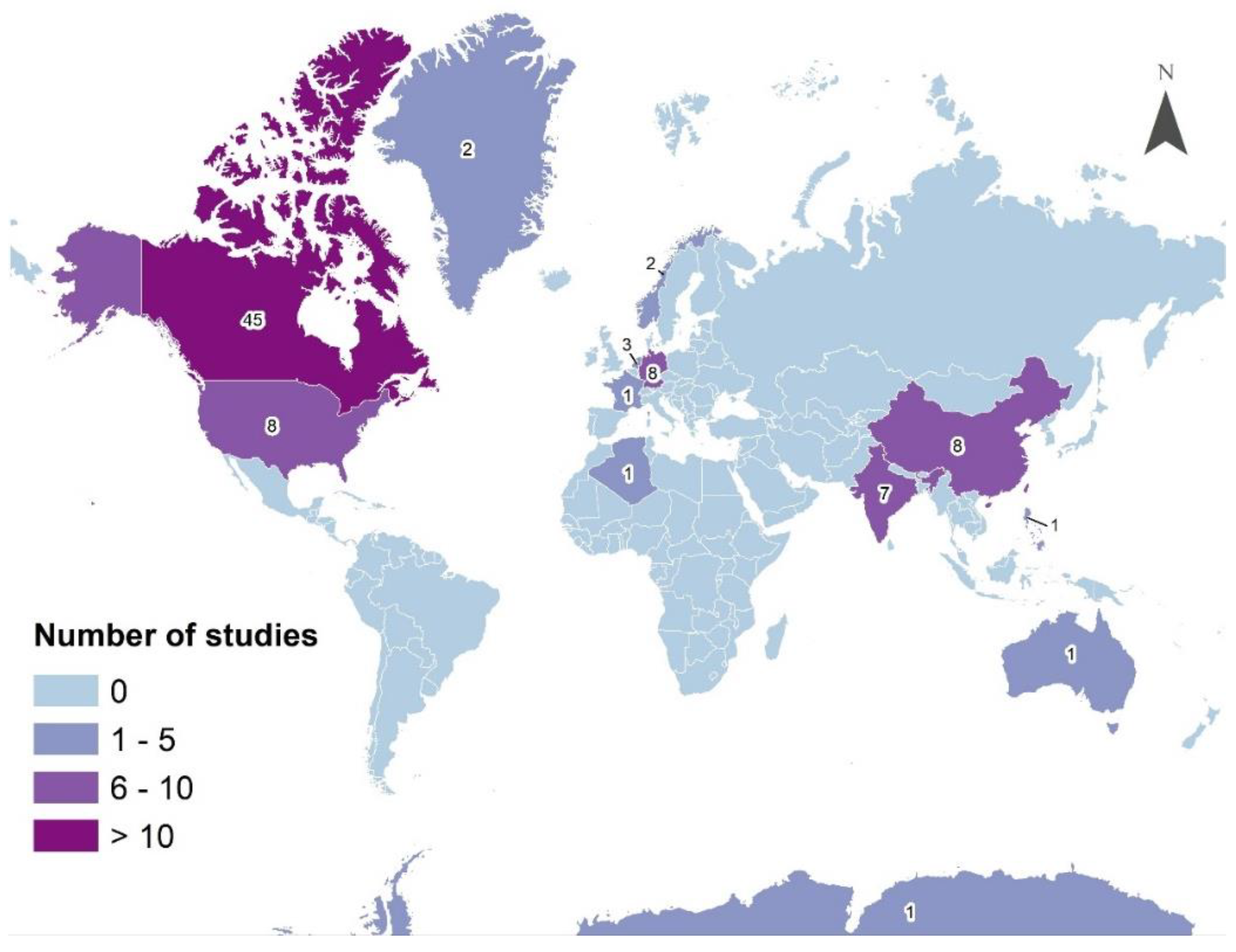
Figure 7 visualizes the number of articles with study areas worldwide. Canada outnumbers other countries by far in terms of the number of studies conducted within its borders, with a total of 45. This is followed by the United States of America, Germany, and China, each with a total of eight, and India with a total of seven. The remaining countries, including Norway, the Netherlands, Greenland, France, Algeria, Australia, and the Philippines, have less than three associated studies. A majority of countries in Europe, Africa, and all countries in South America have not yet any compact polarimetric studies implemented within their borders.
A summary of the overall applications and purposes of the reviewed compact polarimetry articles is outlined in Figure 8. The largest number of articles, at a total of 26, are related to method/technique development and literature reviews, such as the development and testing of novel or modified decomposition techniques, and reviews of various aspects of specific satellites, polarization modes, and decomposition methods. This is followed by applications in the context of oil spill monitoring (12 papers), and target detection and sea ice monitoring (11 papers each). Other common applications include crop monitoring with nine associated papers, soil moisture analysis with seven papers, land cover monitoring and wetland classification with six papers, and vegetation monitoring with five papers. The least common applications of compact polarimetry in the literature include wind characterization and other ice monitoring applications, with four papers each.
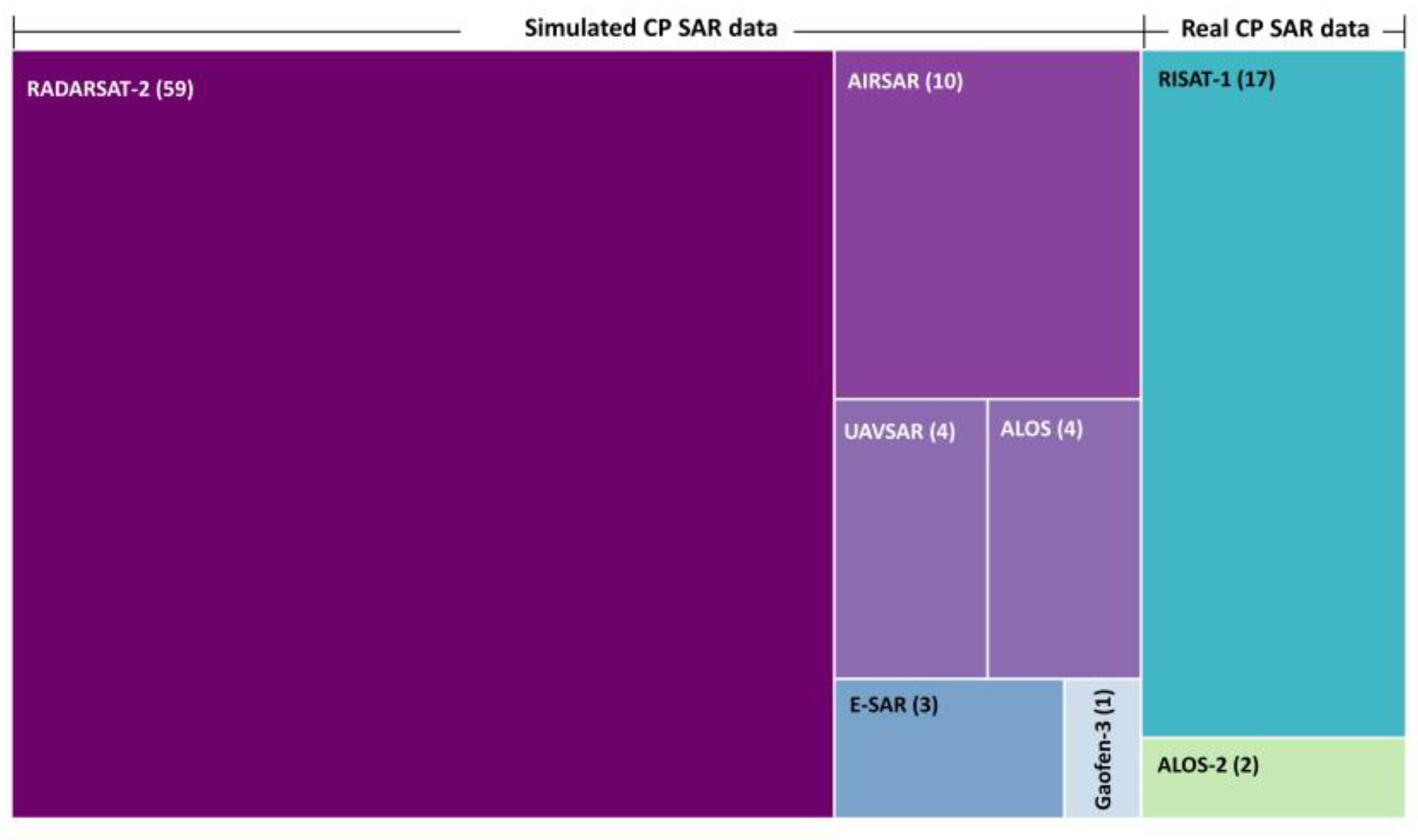
Among these studies, a total of 19 studies used real CP data, 17 of which used RISAT-1 data, by far the most common data source for real compact polarimetry data, and two which used ALOS-2 (Figure 9). However, a majority of the studies, 82 in total, used simulated CP data from a number of different satellites. RADARSAT-2 is the most common source for simulated compact polarimetry data, being used in 59 studies. Other sources of simulated compact polarimetry data include AIRSAR (10 studies), ALOS (4 studies; ALOS-1 & -2), UAVSAR (4 studies), and E-SAR (3 studies each). Data from Gaofen-3 are used in only a single study.
Figure 10 visualizes the use of various decomposition methods in the reviewed studies. Of the total studies, 40% employ the use of the decomposition, followed closely by the decomposition at 37%. In addition, 23% of the studies, almost half of those that used apply the use of Pseudo FP SAR data, despite this practice being advised against. Note that the purpose of a very small number of studies was to derive and apply modified decomposition techniques, the majority of which were applying a modified decomposition.
Generally, image classification techniques, based on the availability of training data, are categorized into unsupervised and supervised classifications. The former approach is preferred when no/insufficient training data are available. Accordingly, finding the most appropriate polarimetric parameters with sufficient information is of great importance for unsupervised PolSAR image classifications. These algorithms have been developed based on target decomposition techniques and polarimetric data distribution theories.
With advances in state-of-the-art artificial intelligence (AI) algorithms, several machine learning classifiers have been applied as a supervised method for FP and HCP SAR image classifications [35,36,38]. Feature extraction is one of the most important steps in supervised PolSAR image classification and has a direct impact on the classification accuracy. Although recent machine learning algorithms allow the user to incorporate a large number of features into the classification step, several studies demonstrated that adding weak and redundant HCP features decreases classification accuracy [35]. Given that maritime surveillance is one the main application of RCM data, the potential of simulated or real HCP SAR data has been well examined for sea ice classification and monitoring in several recent studies [35,62,65]. For example, [62] and [35] examined the discrimination capability of several HCP features extracted from simulated HCP data for sea ice characterization. Similarly, [65] demonstrated the potential of both real HCP data collected from RISAT-1 and simulated HCP data from RADARSAT-2 for sea ice classification.
To date, crop classification in Canada has mostly relied on SAR data, yet the small swath width of FP SAR data hinders the operational capability of such data for this application. Accordingly, the production of annual crop inventories was based on DP SAR data and available optical data. Much gain is expected to be obtained by using HCP SAR data for crop classification. The capability of several HCP SAR data for crop classification has been examined by [29], who reported that the Stokes parameters extracted from simulated HCP data were useful for crop classification. Later, [39] compared the ability of DP, QP, and simulated HCP SAR data for crop classification and identified the most discriminant polarimetric features for classifying various crop classes. With regard to wetland mapping, [66] first reported the potential of HCP SAR data for wetland classification in southwestern Manitoba, Canada, using 12 HCP SAR features. The authors of [63] evaluated the potential of simulated HCP SAR data from RADARSAT-2 with a larger number of HCP features, yet only for peatland classes (i.e., poor fen, open shrub bog, and treed bog) in a small area in southern Ontario, Canada. The authors of [38] demonstrated the capability of 22 simulated HCP SAR data for discriminating Canadian wetland classes and compared wetland classification results of HCP and FP SAR data.
A summary of using different classification methods in CP studies is shown in Figure 11. The most common classification method applied in compact polarimetry studies is the method at 36%. This is followed by the maximum likelihood classifier (MLC) at 25%, random forest classification at 17%, and Support Vector Machine (SVM) at 13%. At 9%, Artificial Neural Network (ANN) is the least commonly applied classification method in the reviewed studies.
A majority of reviewed papers used simulated HCP data, which can be derived from FP data, verses real CP. Most of the simulated HCP SAR data were derived from the RADARSAT-2, real HCP data were obtained using satellites, such as RISAT-1, and sometimes ALOS-2. Applications of real HCP include crop mapping [67,68], sea target detection, ice classification and monitoring [69,70], soil moisture characterization [71], and land cover classification [72,73], among others. Decomposition methods applied in the research listed above most commonly include and .
Some of the research on real HCP also compare HCP results with that of results obtained using FP data [38,39,67,74,75,76]. Generally, a review of this research shows that often HCP and FP obtain comparable results. For example, Singha and Ressel (2017), who used RISAT-1 HCP to characterize sea ice, compared the results of this work with RADARSAT-2 FP data, and found that classification results between the two methods were very similar. Similarly, Uppala et al. (2016) found that the resulting accuracy of RH/RV HCP classification of maize cropland is similar to that of results obtained with FP data. Other research compared classification results using real and simulated HCP, which also generally produced comparable results [69,70]. Espeseth et al. (2017), for example, found that hybrid polarimetric real and simulated have comparable abilities to differentiate sea ice types. While there is currently much less research applying real rather than simulated HCP, it is expected that, with the launch of RCM, the amount of research using real HCP will increase, in addition to its application in novel situations and contexts.
5. Conclusions
Additional polarimetric information collected by PolSAR sensors are beneficial for different environmental monitoring applications in comparison with single-pol SAR data. To date, however, all Earth observation (EO) radar systems have had limitations that impeded operational implementation and acceptance by users of fully polarimetric radar data. As such, RCM has been designed to offer users a suite of operational polarimetric modes. From an operational point of view, the compact polarimetry mode of RCM data that transmits a circularly polarized field (L or R) and receives two orthogonal linear polarizations (H and V) is an optimum polarization mode to collect polarimetric data. The primary image data products from an HCP sensor on RCM are different from those of a traditional polarimetric radar. As such, the processing of RCM’s compact polarimetric data are different from those of conventional polarimetric data. Therefore, there is a need to explore different processing methods that specifically have been designed for HCP data and this review paper was designed to provide an initial response to that need.
As reviewed in this study, several articles that used appropriate methods for processing of HCP SAR data reported the comparable results of HCP SAR sensors to that of full polarimetric SAR. However, some studies used inappropriate methods (e.g., the 3 × 3 pseudo-covariance matrix) for the processing of CP SAR data and then demonstrated the superiority of full polarimetric data compared to CP SAR data. Therefore, our recommendation is to avoid using this method because in general the 3 × 3 pseudo-covariance matrix does not have more information compared to the original 2 × 2 covariance matrix. Another method that should be avoided for CP SAR processing is the decomposition. This is because the decomposition is valid in the case of a perfectly right circular transmission and perfectly calibrated linearly polarized receiver, which are likely not to be true in operational conditions. Such approaches should be avoided. When appropriate methods are used, RCM’s innovative radar architecture supports polarimetry at operational scales.
In this study, a systematic review was also performed by reviewing a total of 101 papers, which used either real or simulated CP SAR data. Canada with 45 studies was the top country in terms of the number of studies using CP SAR data. In addition, CP data were frequently used in oil spill detection, sea ice, and crop mapping. A majority of the studies, 82 in total, used simulated CP data from a number of different satellites. RADARSAT-2 was the most common source for simulated compact polarimetry data. Of great benefit for users, the HCP mode avoids all of the swath coverage limitations of an FP SAR system, while enabling polarimetric feature classifications of comparable quality. Its larger area coverage and frequent revisit capabilities made possible by the HCP aboard RCM allow for sub-weekly observations, thus providing simultaneous high temporal resolution and polarimetric discrimination.
Author Contributions
Conceptualization, B.B., M.M.; writing—original draft, B.B., M.M.; writing—review and editing, B.B., M.M., F.M.; visualization, M.M., F.M.; project administration, M.M.; funding acquisition, M.M. All authors have read and agreed to the published version of the manuscript.
Funding
This research was funded by Natural Resources Canada (CCRS/CCMEO), under Grant number (3000705928) to M.M.
Acknowledgments
The authors would like to thank Francois Charbonneau for a critical review that helped improve the manuscript and Keith Raney for many helpful inputs, comments and reviews.
Conflicts of Interest
The author declares no conflict of interest.
References
- RADARSAT Constellation Mission. Available online: https://www.asc-csa.gc.ca/eng/satellites/radarsat/default.asp (accessed on 21 September 2020).
- Raney, R.K. Hybrid Dual-Polarization Synthetic Aperture Radar. Remote Sens. 2019, 11, 1521. [Google Scholar] [CrossRef] [Green Version]
- Mohammadimanesh, F.; Salehi, B.; Mahdianpari, M.; Brisco, B.; Motagh, M. Wetland Water Level Monitoring Using Interferometric Synthetic Aperture Radar (InSAR): A Review. Can. J. Remote Sens. 2018, 44, 247–262. [Google Scholar] [CrossRef]
- Mahdianpari, M.; Salehi, B.; Mohammadimanesh, F.; Motagh, M. Random forest wetland classification using ALOS-2 L-band, RADARSAT-2 C-band, and TerraSAR-X imagery. ISPRS J. Photogramm. Remote Sens. 2017, 130, 13–31. [Google Scholar] [CrossRef]
- Mahdianpari, M. Advanced Machine Learning Algorithms for Canadian Wetland Mapping Using Polarimetric Synthetic Aperture Radar (PolSAR) and Optical Imagery. Ph.D. Thesis, Memorial University of Newfoundland, St. John’s, NL, Canada, October 2019. [Google Scholar]
- Mahdianpari, M.; Brisco, B.; Granger, J.E.; Mohammadimanesh, F.; Salehi, B.; Banks, S.; Homayouni, S.; Bourgeau-Chavez, L.; Weng, Q. The Second Generation Canadian Wetland Inventory Map at 10 Meters Resolution Using Google Earth Engine. Can. J. Remote Sens. 2020, 46, 360–375. [Google Scholar] [CrossRef]
- Ban, Y.; Zhang, P.; Nascetti, A.; Bevington, A.R.; Wulder, M.A. Near Real-Time Wildfire Progression Monitoring with Sentinel-1 SAR Time Series and Deep Learning. Sci. Rep. 2020, 10, 1–15. [Google Scholar] [CrossRef] [Green Version]
- Salberg, A.-B.; Rudjord, O.; Solberg, A.H.S. Oil Spill Detection in Hybrid-Polarimetric SAR Images. IEEE Trans. Geosci. Remote Sens. 2014, 52, 6521–6533. [Google Scholar] [CrossRef]
- Yin, J.; Yang, J.; Zhou, Z.-S.; Song, J. The Extended Bragg Scattering Model-Based Method for Ship and Oil-Spill Observation Using Compact Polarimetric SAR. IEEE J. Sel. Top. Appl. Earth Obs. Remote Sens. 2014, 8, 3760–3772. [Google Scholar] [CrossRef]
- Zakhvatkina, N.; Smirnov, V.G.; Bychkova, I. Satellite SAR Data-based Sea Ice Classification: An Overview. Geoscience 2019, 9, 152. [Google Scholar] [CrossRef] [Green Version]
- Shirvany, R.; Chabert, M.; Tourneret, J.-Y. Ship and Oil-Spill Detection Using the Degree of Polarization in Linear and Hybrid/Compact Dual-Pol SAR. IEEE J. Sel. Top. Appl. Earth Obs. Remote Sens. 2012, 5, 885–892. [Google Scholar] [CrossRef] [Green Version]
- Touzi, R.; Vachon, P.W. RCM Polarimetric SAR for Enhanced Ship Detection and Classification. Can. J. Remote Sens. 2015, 41, 473–484. [Google Scholar] [CrossRef]
- Olsen, R.B.; Wahl, T. The role of wide swath SAR in high-latitude coastal management. Johns Hopkins APL Tech. Dig. 2000, 21, 136–140. [Google Scholar]
- Mahdianpari, M.; Salehi, B.; Mohammadimanesh, F.; Homayouni, S.; Gill, E.W. The First Wetland Inventory Map of Newfoundland at a Spatial Resolution of 10 m Using Sentinel-1 and Sentinel-2 Data on the Google Earth Engine Cloud Computing Platform. Remote Sens. 2018, 11, 43. [Google Scholar] [CrossRef] [Green Version]
- Joshi, N.; Baumann, M.; Ehammer, A.; Fensholt, R.; Grogan, K.; Hostert, P.; Jepsen, M.R.; Kuemmerle, T.; Meyfroidt, P.; Mitchard, E.T.A.; et al. A Review of the Application of Optical and Radar Remote Sensing Data Fusion to Land Use Mapping and Monitoring. Remote Sens. 2016, 8, 70. [Google Scholar] [CrossRef] [Green Version]
- Mohammadimanesh, F.; Salehi, B.; Mahdianpari, M.; Brisco, B.; Motagh, M. Multi-temporal, multi-frequency, and multi-polarization coherence and SAR backscatter analysis of wetlands. ISPRS J. Photogramm. Remote Sens. 2018, 142, 78–93. [Google Scholar] [CrossRef]
- Souyris, J.-C.; Imbo, P.; Fjortoft, R.; Mingot, S.; Lee, J.-S. Compact polarimetry based on symmetry properties of geophysical media: The /spl pi//4 mode. IEEE Trans. Geosci. Remote Sens. 2005, 43, 634–646. [Google Scholar] [CrossRef]
- Mohammadimanesh, F.; Salehi, B.; Mahdianpari, M.; Gill, E.; Molinier, M. A new fully convolutional neural network for semantic segmentation of polarimetric SAR imagery in complex land cover ecosystem. ISPRS J. Photogramm. Remote Sens. 2019, 151, 223–236. [Google Scholar] [CrossRef]
- Mohammadimanesh, F.; Salehi, B.; Mahdianpari, M.; Homayouni, S. Unsupervised wishart classfication of wetlands in Newfoundland, Canada using polsar data based on fisher linear discriminant analysis. Int. Arch. Photogramm. Remote Sens. Spat. Inf. Sci. 2016, 41, 305–310. [Google Scholar] [CrossRef]
- Lee, J.-S.; Pottier, E. Polarimetric Radar Imaging: From Basics to Applications; CRC Press: Boca Raton, FL, USA, 2009. [Google Scholar]
- Boerner, W.M. PolSARPro v3. 0-Lecture Notes, Basic Concepts in Radar Polarimetry; European Space Agency: Noordwijk, The Netherlands, 2010.
- Van Zyl, J.J.; Zebker, H.A.; Elachi, C. Imaging radar polarization signatures: Theory and observation. Radio Sci. 1987, 22, 529–543. [Google Scholar] [CrossRef]
- Mahdianpari, M.; Salehi, B.; Mohammadimanesh, F. The Effect of PolSAR Image De-speckling on Wetland Classification: Introducing a New Adaptive Method. Can. J. Remote Sens. 2017, 43, 485–503. [Google Scholar] [CrossRef]
- Van Zyl, J.J. Synthetic Aperture Radar Polarimetry; John Wiley & Sons: Hoboken, NJ, USA, 2011; Volume 2. [Google Scholar]
- Buono, A.; Nunziata, F.; Migliaccio, M. Analysis of Full and Compact Polarimetric SAR Features Over the Sea Surface. IEEE Geosci. Remote Sens. Lett. 2016, 13, 1527–1531. [Google Scholar] [CrossRef]
- Ainsworth, T.; Kelly, J.; Lee, J.-S. Classification comparisons between dual-pol, compact polarimetric and quad-pol SAR imagery. ISPRS J. Photogramm. Remote Sens. 2009, 64, 464–471. [Google Scholar] [CrossRef]
- Fobert, M.-A.; Spray, J.G.; Singhroy, V. Assessing the Benefits of Simulated RADARSAT Constellation Mission Polarimetry Images for Structural Mapping of an Impact Crater in the Canadian Shield. Can. J. Remote Sens. 2018, 44, 321–336. [Google Scholar] [CrossRef] [Green Version]
- Raney, R.K. Comparing Compact and Quadrature Polarimetric SAR Performance. IEEE Geosci. Remote Sens. Lett. 2016, 13, 861–864. [Google Scholar] [CrossRef]
- Charbonneau, F.J.; Brisco, B.; Raney, R.K.; McNairn, H.; Liu, C.; Vachon, P.W.; Shang, J.; DeAbreu, R.; Champagne, C.; Merzouki, A.; et al. Compact polarimetry overview and applications assessment. Can. J. Remote Sens. 2010, 36, S298–S315. [Google Scholar] [CrossRef]
- Mahdianpari, M.; Salehi, B.; Mohammadimanesh, F.; Brisco, B. An Assessment of Simulated Compact Polarimetric SAR Data for Wetland Classification Using Random Forest Algorithm. Can. J. Remote Sens. 2017, 43, 468–484. [Google Scholar] [CrossRef]
- Sabry, R.; Vachon, P.W. A Unified Framework for General Compact and Quad Polarimetric SAR Data and Imagery Analysis. IEEE Trans. Geosci. Remote Sens. 2013, 52, 582–602. [Google Scholar] [CrossRef]
- Stokes, G.G. On the composition and resolution of streams of polarized light from different sources. Trans. Camb. Philos. Soc. 1851, 9, 399. [Google Scholar]
- Raney, R.K.; Spudis, P.D.; Bussey, B.; Crusan, J.; Jensen, J.R.; Marinelli, W.; McKerracher, P.; Neish, C.; Palsetia, M.; Schulze, R.; et al. The Lunar Mini-RF Radars: Hybrid Polarimetric Architecture and Initial Results. Proc. IEEE 2011, 99, 808–823. [Google Scholar] [CrossRef]
- Raney, R.K.; Cahill, J.T.; Patterson, G.; Bussey, D.B.J. The m-chi decomposition of hybrid dual-polarimetric radar data with application to lunar craters. J. Geophys. Res. Planets 2012, 117. [Google Scholar] [CrossRef]
- Dabboor, M.; Geldsetzer, T. Towards sea ice classification using simulated RADARSAT Constellation Mission compact polarimetric SAR imagery. Remote Sens. Environ. 2014, 140, 189–195. [Google Scholar] [CrossRef]
- Aghabalaei, A.; Maghsoudi, Y.; Ebadi, H. Forest classification using extracted PolSAR features from Compact Polarimetry data. Adv. Space Res. 2016, 57, 1939–1950. [Google Scholar] [CrossRef]
- Dabboor, M.; Singha, S.; Montpetit, B.; Deschamps, B.; Flett, D. Pre-Launch Assessment of RADARSAT Constellation Mission Medium Resolution Modes for Sea Oil Slicks and Lookalike Discrimination. Can. J. Remote Sens. 2019, 45, 530–549. [Google Scholar] [CrossRef] [Green Version]
- Mohammadimanesh, F.; Salehi, B.; Mahdianpari, M.; Brisco, B.; Gill, E.W. Full and Simulated Compact Polarimetry SAR Responses to Canadian Wetlands: Separability Analysis and Classification. Remote Sens. 2019, 11, 516. [Google Scholar] [CrossRef] [Green Version]
- Mahdianpari, M.; Mohammadimanesh, F.; McNairn, H.; Davidson, A.; Rezaee, M.; Salehi, B.; Homayouni, S. Mid-season Crop Classification Using Dual-, Compact-, and Full-polarization in Preparation for the Radarsat Constellation Mission (RCM). Remote Sens. 2019, 11, 1582. [Google Scholar] [CrossRef] [Green Version]
- Mathews, J.D. A short history of geophysical radar at Arecibo Observatory. Hist. Geo-Space Sci. 2013, 4, 19–33. [Google Scholar] [CrossRef] [Green Version]
- De Lisle, D.; Iris, S.; Arsenault, E.; Smyth, J.; Kroupnik, G. RADARSAT constellation mission status update. In Proceedings of the 12th European Conference on Synthetic Aperture Radar, Aachen, Germany, 4–7 June 2018; pp. 1–5. [Google Scholar]
- Harati-Mokhtari, A.; Wall, A.; Brookes, P.; Wang, J. Automatic Identification System (AIS): A human factors approach. J. Navig. 2007, 60, 373–389. [Google Scholar] [CrossRef]
- Cloude, S.R. A General Elliptical Formulation of Hybrid-POLSAR System Ambiguities. IEEE Geosci. Remote Sens. Lett. 2019, 16, 1066–1069. [Google Scholar] [CrossRef]
- Boularbah, S.; Ouarzeddine, M.; Belhadj-Aissa, A. Investigation of the capability of the Compact Polarimetry mode to Reconstruct Full Polarimetry mode using RADARSAT2 data. Adv. Electromagn. 2012, 1, 19–28. [Google Scholar] [CrossRef] [Green Version]
- Raney, R. Hybrid-Polarity SAR Architecture. IEEE Trans. Geosci. Remote Sens. 2007, 45, 3397–3404. [Google Scholar] [CrossRef] [Green Version]
- Truong-LoI, M.-L.; Freeman, A.; Dubois-Fernandez, P.; Pottier, E. Estimation of Soil Moisture and Faraday Rotation from Bare Surfaces Using Compact Polarimetry. IEEE Trans. Geosci. Remote Sens. 2009, 47, 3608–3615. [Google Scholar] [CrossRef]
- Singha, S.; Ressel, R. Arctic Sea Ice Characterization Using RISAT-1 Compact-Pol SAR Imagery and Feature Evaluation: A Case Study Over Northeast Greenland. IEEE J. Sel. Top. Appl. Earth Obs. Remote Sens. 2017, 10, 3504–3514. [Google Scholar] [CrossRef] [Green Version]
- Kumar, V.; McNairn, H.; Bhattacharya, A.; Rao, Y.S. Temporal Response of Scattering from Crops for Transmitted Ellipticity Variation in Simulated Compact-Pol SAR Data. IEEE J. Sel. Top. Appl. Earth Obs. Remote Sens. 2017, 10, 5163–5174. [Google Scholar] [CrossRef]
- Van Zyl, J. Unsupervised classification of scattering behavior using radar polarimetry data. IEEE Trans. Geosci. Remote Sens. 1989, 27, 36–45. [Google Scholar] [CrossRef]
- Freeman, A.; Durden, S. A three-component scattering model for polarimetric SAR data. IEEE Trans. Geosci. Remote Sens. 1998, 36, 963–973. [Google Scholar] [CrossRef] [Green Version]
- Yamaguchi, Y.; Moriyama, T.; Ishido, M.; Yamada, H. Four-component scattering model for polarimetric SAR image decomposition. IEEE Trans. Geosci. Remote Sens. 2005, 43, 1699–1706. [Google Scholar] [CrossRef]
- Pottier, E.; Cloude, S.R. Application of the H/A/alpha polarimetric decomposition theorem for land classification. In Proceedings of the Wideband Interferometric Sensing and Imaging Polarimetry; International Society for Optics and Photonics, San Diego, CA, USA, 8–14 February 1997; Volume 3120, pp. 132–143. [Google Scholar]
- Touzi, R. Target Scattering Decomposition in Terms of Roll-Invariant Target Parameters. IEEE Trans. Geosci. Remote Sens. 2007, 45, 73–84. [Google Scholar] [CrossRef]
- Doulgeris, A.P.; Anfinsen, S.N.; Eltoft, T. Classification with a Non-Gaussian Model for PolSAR Data. IEEE Trans. Geosci. Remote Sens. 2008, 46, 2999–3009. [Google Scholar] [CrossRef] [Green Version]
- Yueh, S.; Kong, J.; Jao, J.; Shin, R.; Novak, L. K-Distribution and Polarimetric Terrain Radar Clutter. J. Electromagn. Waves Appl. 1989, 3, 747–768. [Google Scholar] [CrossRef]
- Lee, J.S.; Schuler, D.L.; Lang, R.H.; Ranson, K.J. K-distribution for multi-look processed polarimetric SAR imagery. In Proceedings of the IEEE International Geoscience and Remote Sensing Symposium (IGARSS’94-1994), Mono Lake, CA, USA, 8–12 August 1994; Volume 4, pp. 2179–2181. [Google Scholar]
- Cloude, S.R.; Goodenough, D.G.; Chen, H. Compact decomposition theory for L-Band satellite radar applications. In Proceedings of the 2012 IEEE International Geoscience and Remote Sensing Symposium, Munich, Germany, 22–27 July 2012; pp. 5097–5100. [Google Scholar]
- Li, H.; Perrie, W. Sea Ice Characterization and Classification Using Hybrid Polarimetry SAR. IEEE J. Sel. Top. Appl. Earth Obs. Remote Sens. 2016, 9, 4998–5010. [Google Scholar] [CrossRef]
- Kumar, A.; Das, A.; Panigrahi, R.K. Hybrid-Pol Based Three-Component Scattering Model for Analysis of RISAT Data. IEEE J. Sel. Top. Appl. Earth Obs. Remote Sens. 2017, 10, 5155–5162. [Google Scholar] [CrossRef]
- Harmon, J.K.; Perillat, P.J.; Slade, M.A. High-resolution radar imaging of Mercury’s north pole. Icarus 2001, 149, 1–15. [Google Scholar] [CrossRef]
- Campbell, B.; Neish, C.; Campbell, D.; Carter, L.; Morgan, G.; Nolan, M.; Patterson, G.W.; Rivera-Valentin, E.; Taylor, P.; Whitten, J. Radar Astronomy for Planetary Surface Studies. Astro2020 Sci. White Pap. 2019, BAAS 51, 350. [Google Scholar]
- Geldsetzer, T.; Arkett, M.; Zagon, T.; Charbonneau, F.; Yackel, J.J.; Scharien, R. All-season Compact-Polarimetry C-band SAR Observations of Sea Ice. Can. J. Remote Sens. 2015, 41, 485–504. [Google Scholar] [CrossRef]
- White, L.; Millard, K.; Banks, S.; Richardson, M.; Pasher, J.; Duffe, J. Moving to the RADARSAT Constellation Mission: Comparing Synthesized Compact Polarimetry and Dual Polarimetry Data with Fully Polarimetric RADARSAT-2 Data for Image Classification of Peatlands. Remote Sens. 2017, 9, 573. [Google Scholar] [CrossRef] [Green Version]
- Moher, D.; Liberati, A.; Tetzlaff, J.; Altman, D.G. Preferred reporting items for systematic reviews and meta-analyses: The PRISMA statement. Ann. Intern. Med. 2009, 151, 264–269. [Google Scholar] [CrossRef] [PubMed] [Green Version]
- Espeseth, M.M.; Brekke, C.; Johansson, A.M. Assessment of RISAT-1 and Radarsat-2 for Sea Ice Observations from a Hybrid-Polarity Perspective. Remote Sens. 2017, 9, 1088. [Google Scholar] [CrossRef] [Green Version]
- Brisco, B.; Li, K.; Tedford, B.; Charbonneau, F.; Yun, S.; Murnaghan, K. Compact polarimetry assessment for rice and wetland mapping. Int. J. Remote Sens. 2012, 34, 1949–1964. [Google Scholar] [CrossRef] [Green Version]
- Uppala, D.; Venkata, R.K.; Poloju, S.; Rama, S.M.V.; Dadhwal, V.K. Discrimination of maize crop with hybrid polarimetric RISAT1 data. Int. J. Remote Sens. 2016, 37, 2641–2652. [Google Scholar] [CrossRef]
- Uppala, D.; Kothapalli, R.V.; Poloju, S.; Mullapudi, S.S.V.R.; Dadhwal, V.K. Rice Crop Discrimination Using Single Date RISAT1 Hybrid (RH, RV) Polarimetric Data. Photogramm. Eng. Remote Sens. 2015, 81, 557–563. [Google Scholar] [CrossRef]
- Paes, R.L.; Buono, A.; Nunziata, F.; Migliaccio, M. On the Sensitivity Analysis of the Compact-Polarimetry SAR Architectures for Maritime Targets Detection; Bostater, C.R., Mertikas, S.P., Neyt, X., Eds.; Remote Sensing of the Ocean, Sea Ice, Coastal Waters, and Large Water Regions; International Society for Optics and Photonics: Amsterdam, The Netherlands, 2014; p. 92401A. [Google Scholar]
- Singha, S. Potential of Compact Polarimetry for Operational Sea Ice Monitoring Over Arctic and Antarctic Region. In Proceedings of the IEEE International Geoscience and Remote Sensing Symposium (IGARSS 2018), Valencia, Spain, 22–27 July 2018; pp. 7113–7116. [Google Scholar]
- Ponnurangam, G.G.; Jagdhuber, T.; Hajnsek, I.; Rao, Y.S. Soil Moisture Estimation Using Hybrid Polarimetric SAR Data of RISAT-1. IEEE Trans. Geosci. Remote Sens. 2016, 54, 2033–2049. [Google Scholar] [CrossRef]
- Dasari, K.; Lokam, A. Exploring the Capability of Compact Polarimetry (Hybrid Pol) C Band RISAT-1 Data for Land Cover Classification. IEEE Access 2018, 6, 57981–57993. [Google Scholar] [CrossRef]
- Sabry, R.; Ainsworth, T.L. SAR Compact Polarimetry for Change Detection and Characterization. IEEE J. Sel. Top. Appl. Earth Obs. Remote Sens. 2019, 12, 898–909. [Google Scholar] [CrossRef]
- Buono, A.; Nunziata, F.; Migliaccio, M.; Li, X. Polarimetric Analysis of Compact-Polarimetry SAR Architectures for Sea Oil Slick Observation. IEEE Trans. Geosci. Remote Sens. 2016, 54, 5862–5874. [Google Scholar] [CrossRef]
- Atteia, G.; Collins, M. Ship detection performance using simulated dual-polarization RADARSAT constellation mission data. Int. J. Remote Sens. 2015, 36, 1705–1727. [Google Scholar] [CrossRef]
- Kumar, A.; Das, A.; Panigrahi, R.K. Hybrid-pol Decomposition Methods: A Comparative Evaluation and a New Entropy-based Approach. IETE Tech. Rev. 2019, 37, 296–308. [Google Scholar] [CrossRef]
Figure 1.
Three compact polarimetric Synthetic Aperture Radar (SAR) modes.

Figure 2.
RADARSAT Constellation Mission (RCM) imaging modes. All of RCM’s operational modes are hybrid compact polarimetric--including ScanSAR, which is a major paradigm shift for Earth Observation (EO) SARs [1].
Figure 2.
RADARSAT Constellation Mission (RCM) imaging modes. All of RCM’s operational modes are hybrid compact polarimetric--including ScanSAR, which is a major paradigm shift for Earth Observation (EO) SARs [1].

Figure 3.
The geometrical relationship between Stokes and Poincaré parameters.

Figure 4.
An RGB color wheel of seven-fold classification. Adapted from [34].
Figure 4.
An RGB color wheel of seven-fold classification. Adapted from [34].

Figure 5.
All the possible values of the of a target interacting with a circular wave [29].
Figure 5.
All the possible values of the of a target interacting with a circular wave [29].

Figure 6.
Flowchart of the literature selection process.

Figure 7.
Number of compact polarimetry studies conducted within countries across the globe.

Figure 8.
Applications of compact polarimetry in the literature.

Figure 9.
Number of studies that used real or simulated compact polarimetry data.

Figure 10.
Different decomposition methods used for Hybrid Compact Polarimetry (HCP) data analysis.

Figure 11.
Most common classification methods applied to CP data.


Table 1.
Meta-analysis database attributes.
| Attribute | Type | Category |
|---|---|---|
| First Author | Text | |
| Year | Numeric | |
| Publication | Text | |
| Title | Text | |
| Document Type | Text | Article, Conference, Review, Letter |
| Country | Text | |
| Polarization Mode | Class | π/4, CTLR, HCP |
| Simulated or Real | Class | Simulated, Real |
| Pseudo Quad | Class | Yes, No |
| Comparison of results with full or dual | Class | Full, Dual, Both |
| Classification Method | Class | classification, SVM, MLC, ANN, Random Forest, Thresholding |
| Decomposition Method | Class | , |
| Resolution | Numeric | |
| Features | List | Stokes Vector Components, like- and cross-polarized radar, degree of polarization (m), circular-polarization ratio (CPR), degree of linear polarization, polarization ratio, correlation coefficient, decomposition parameters, phase difference, conformity, alpha angle etc. |
| Number of Features | Numeric |
© 2020 by the authors. Licensee MDPI, Basel, Switzerland. This article is an open access article distributed under the terms and conditions of the Creative Commons Attribution (CC BY) license (http://creativecommons.org/licenses/by/4.0/).
Share and Cite
MDPI and ACS Style
Brisco, B.; Mahdianpari, M.; Mohammadimanesh, F. Hybrid Compact Polarimetric SAR for Environmental Monitoring with the RADARSAT Constellation Mission. Remote Sens. 2020, 12, 3283. https://0-doi-org.brum.beds.ac.uk/10.3390/rs12203283
AMA Style
Brisco B, Mahdianpari M, Mohammadimanesh F. Hybrid Compact Polarimetric SAR for Environmental Monitoring with the RADARSAT Constellation Mission. Remote Sensing. 2020; 12(20):3283. https://0-doi-org.brum.beds.ac.uk/10.3390/rs12203283
Chicago/Turabian StyleBrisco, Brian, Masoud Mahdianpari, and Fariba Mohammadimanesh. 2020. "Hybrid Compact Polarimetric SAR for Environmental Monitoring with the RADARSAT Constellation Mission" Remote Sensing 12, no. 20: 3283. https://0-doi-org.brum.beds.ac.uk/10.3390/rs12203283
Note that from the first issue of 2016, this journal uses article numbers instead of page numbers. See further details here.