Assessment of the Accuracy of the Saastamoinen Model and VMF1/VMF3 Mapping Functions with Respect to Ray-Tracing from Radiosonde Data in the Framework of GNSS Meteorology


Abstract
:
1. Introduction
2. Data and Methodology
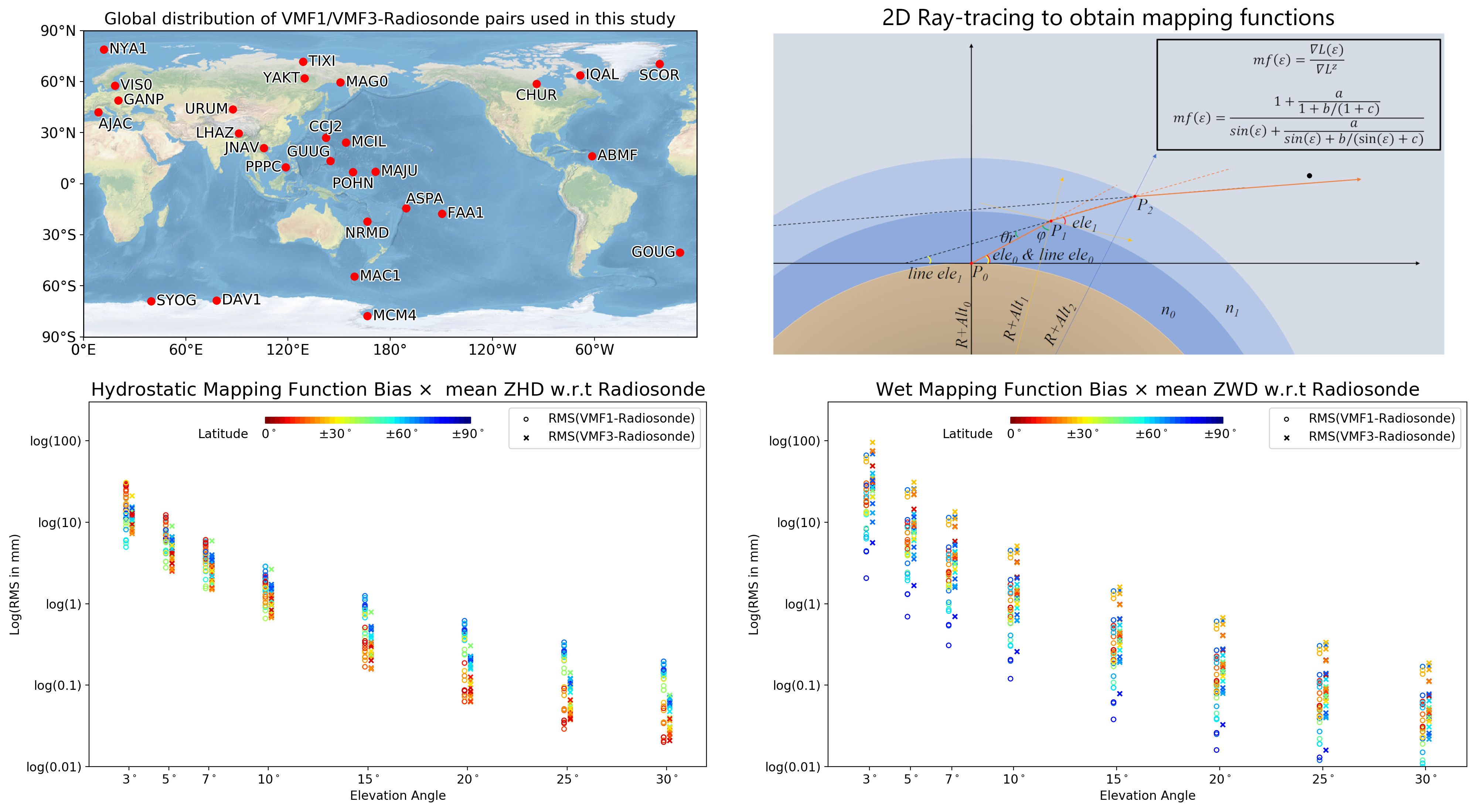
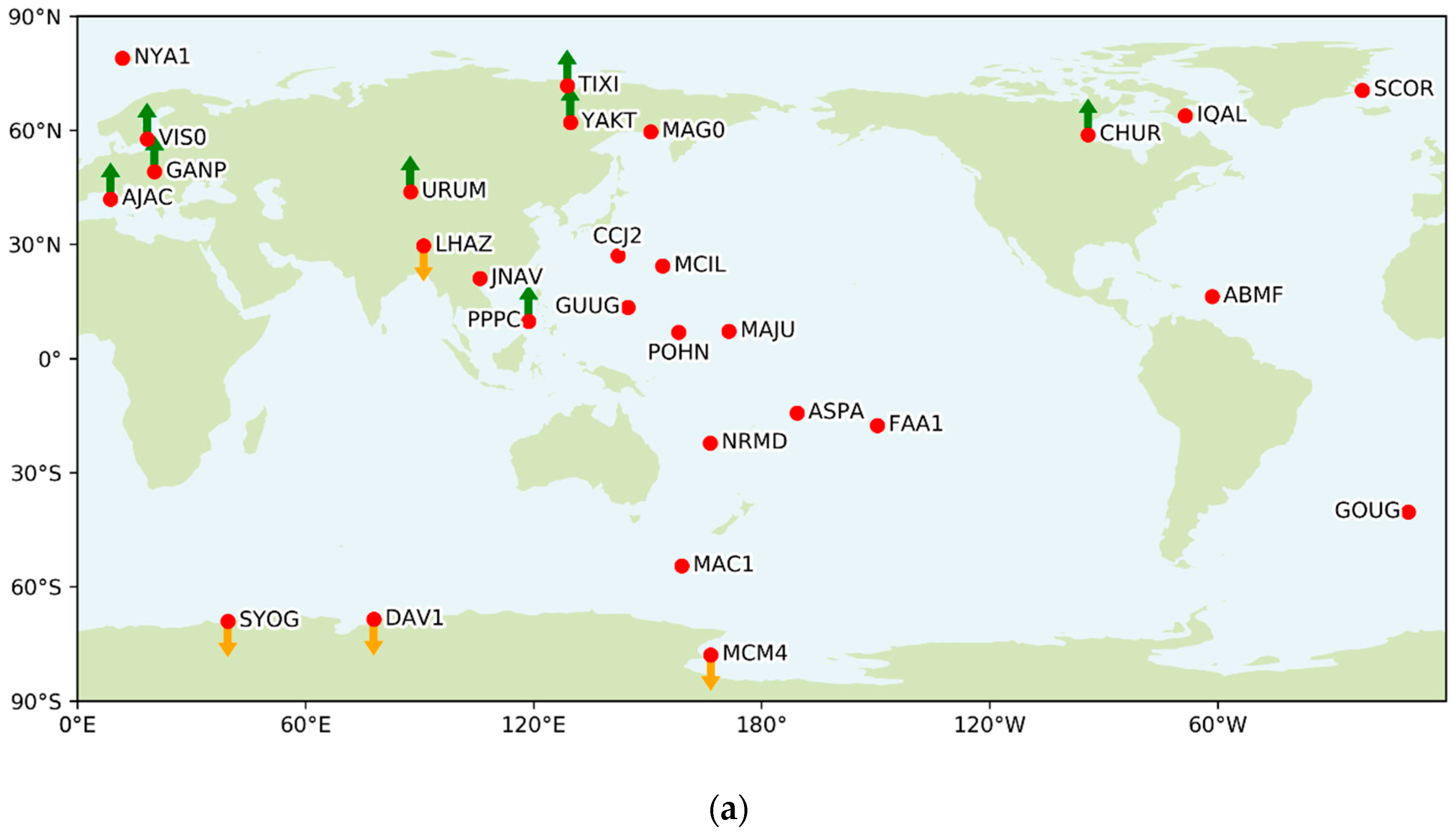
2.1. Radiosonde Data
2.2. Data Interpolation and Extension
2.3. Refractivity and Ray-Tracing
3. Results: ZHD Comparison
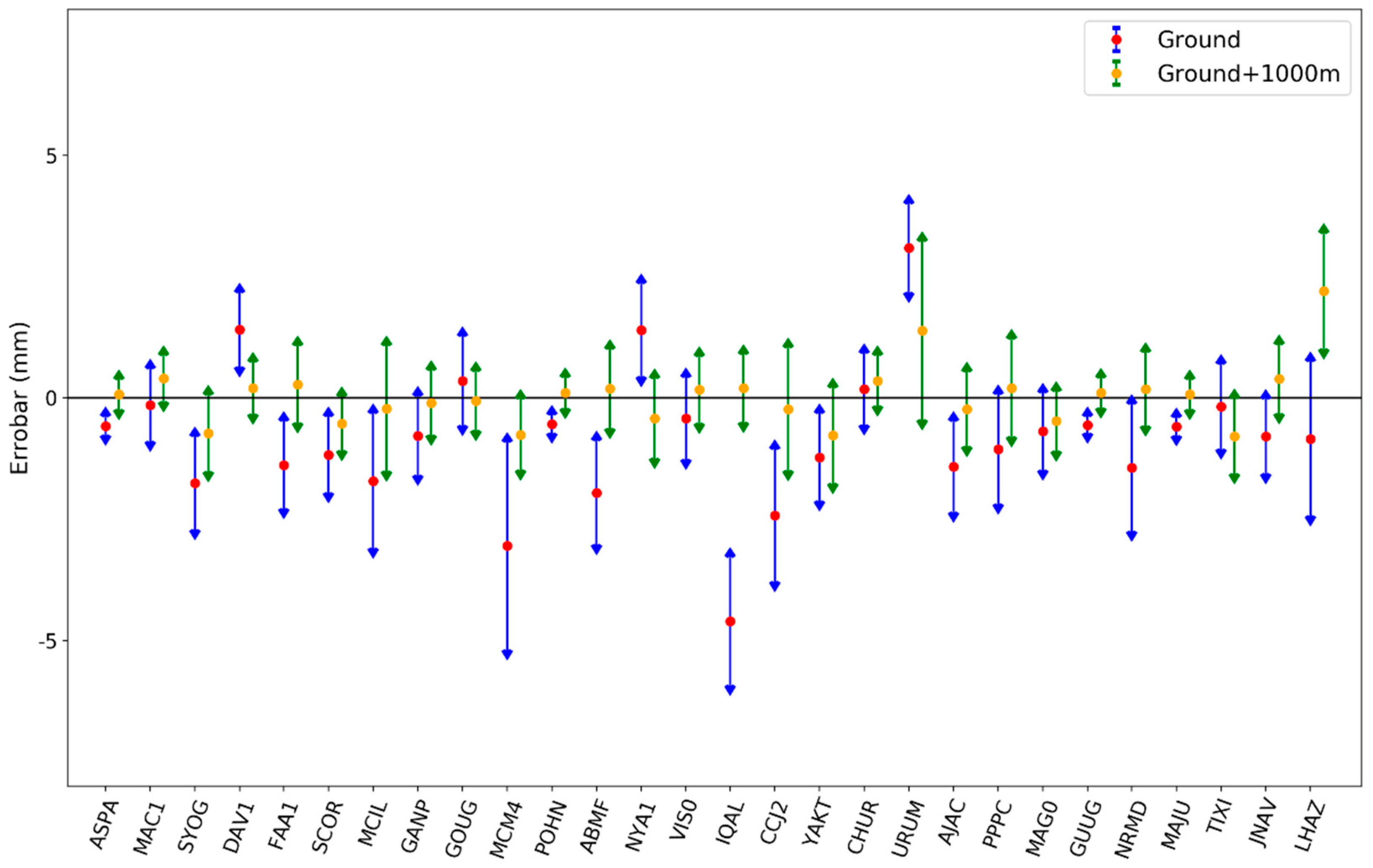
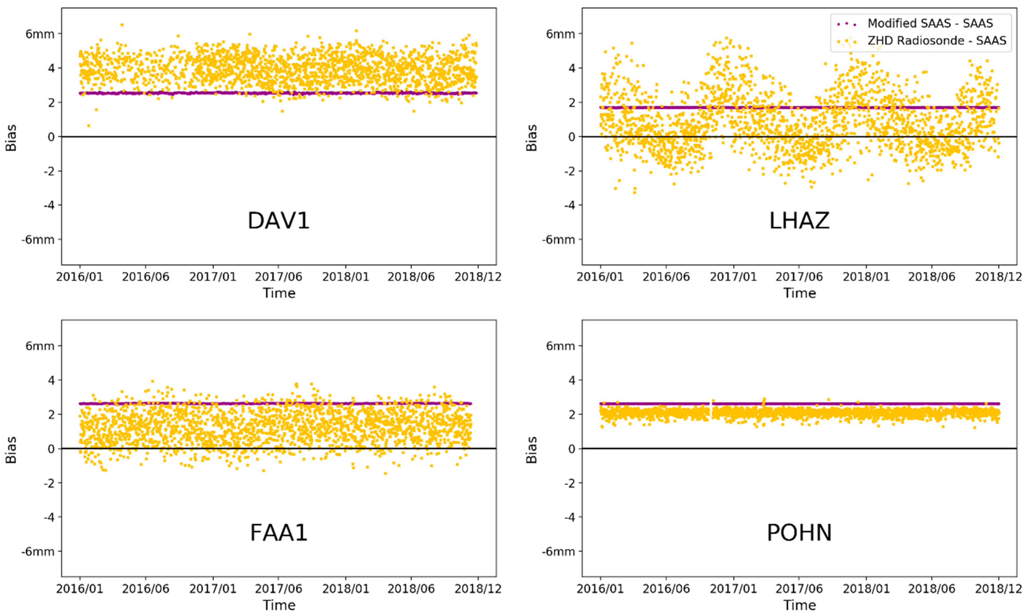
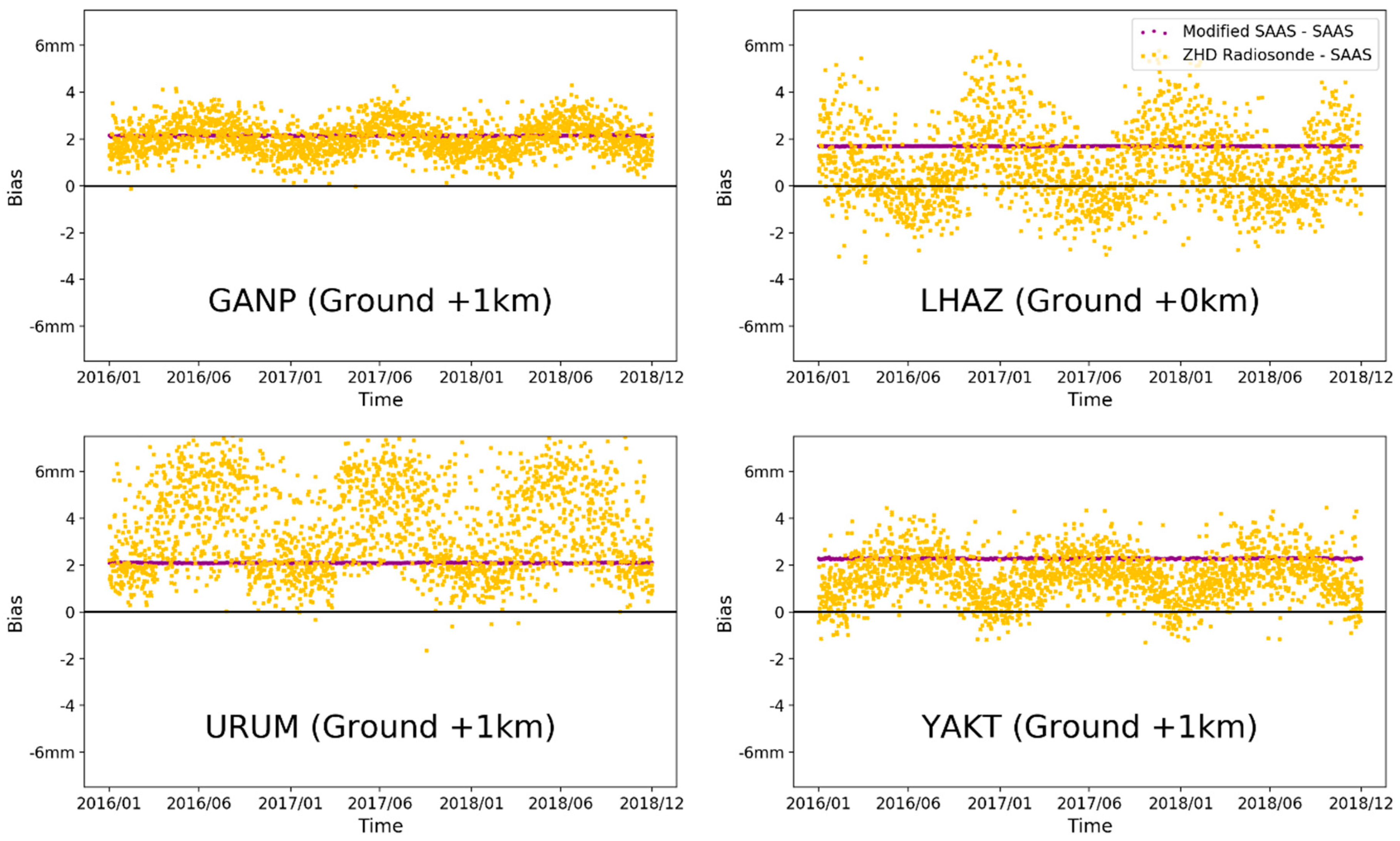
3.1. Accuracy of Saastamoinen ZHD Model
3.2. Seasonal Bias in the Saastamoinen ZHD
4. Results: Mapping Function Comparison
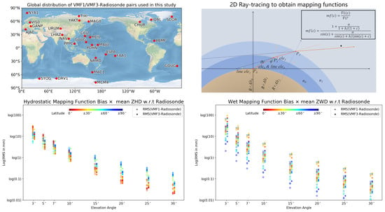
4.1. Hydrostatic Mapping Function

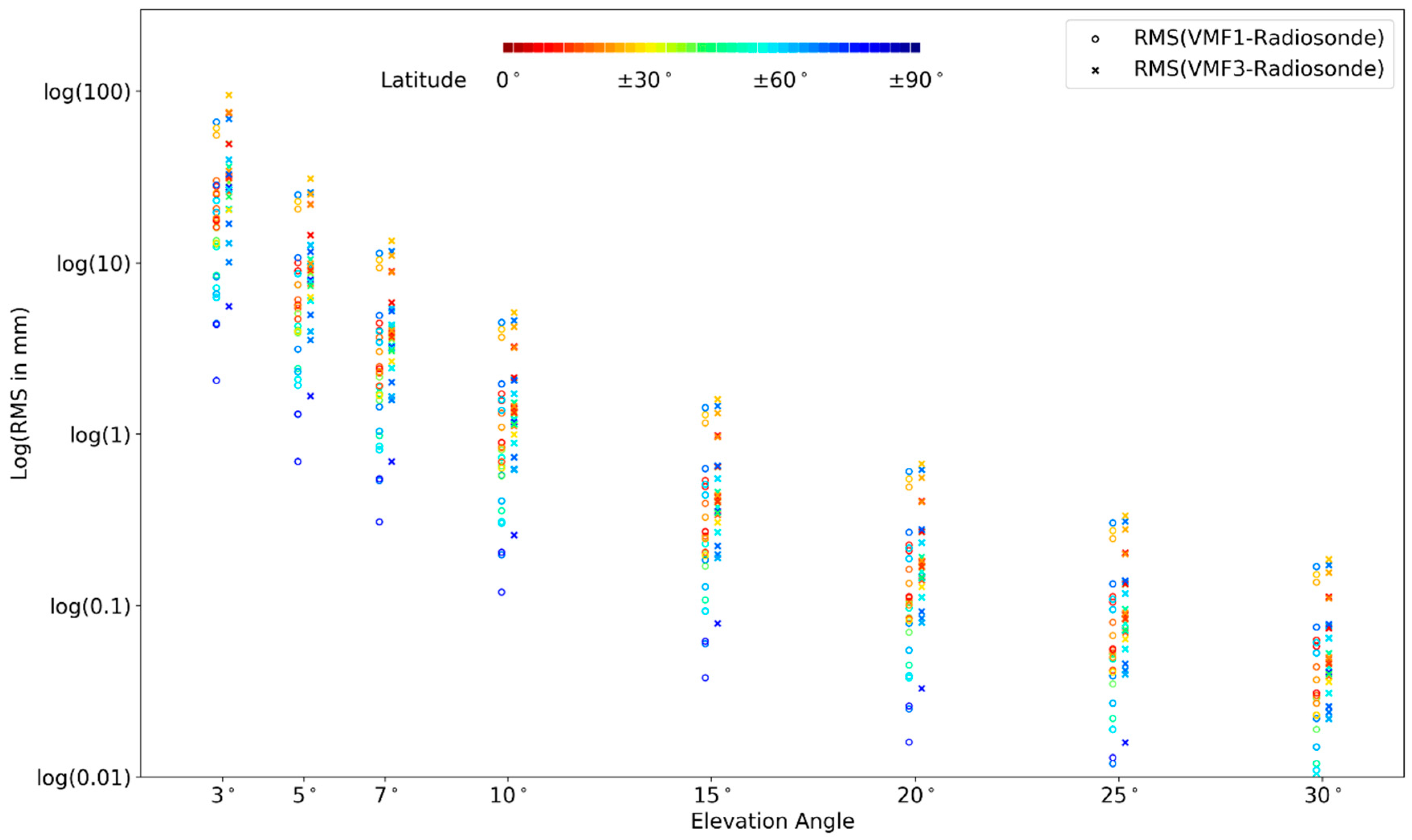
| Elevation Angle | 30° | 25° | 20° | 15° | 10° | 7° | 5° | 3° |
|---|---|---|---|---|---|---|---|---|
| RMS (VMF1) | 0.10 | 0.16 | 0.30 | 0.61 | 1.7 | 3.8 | 7.1 | 15.8 |
| RMS (VMF3) | 0.05 | 0.08 | 0.15 | 0.36 | 1.2 | 2.7 | 4.8 | 11.6 |
| Bias (VMF1) | −0.09 | −0.14 | −0.23 | −0.37 | −0.31 | 0.42 | 1.1 | 6.2 |
| Bias (VMF3) | −0.02 | −0.02 | −0.01 | 0.08 | 0.62 | 1.4 | 0.4 | 2.5 |
| STD (VMF1) | 0.04 | 0.07 | 0.15 | 0.33 | 0.91 | 1.9 | 3.3 | 6.5 |
| STD (VMF3) | 0.04 | 0.07 | 0.14 | 0.31 | 0.92 | 2.1 | 4.2 | 10.3 |
| post-fit STD (VMF1) | 0.03 | 0.05 | 0.11 | 0.24 | 0.70 | 1.6 | 2.9 | 6.3 |
| post-fit STD (VMF3) | 0.03 | 0.06 | 0.11 | 0.26 | 0.75 | 1.8 | 3.5 | 9.0 |
4.2. Wet Mapping Function
5. Conclusions
Author Contributions
Funding
Acknowledgments
Conflicts of Interest
References
- Herring, T.A.; King, R.W.; Floyd, M.A.; McClusky, S.C. GAMIT Reference Manual: GPS Analysis at MIT, Release 10.6; Massachusetts Institute of Technology: Cambridge, MA, USA, 2010; ISBN 0099-2240. [Google Scholar]
- Dach, R.; Lutz, S.; Walser, P.; Fridez, P. (Eds.) Bernese GNSS Software Version 5.2; University of Bern, Bern Open Publishing: Bern, Switzerland, 2015; Volume 2, ISBN 1879621142. [Google Scholar]
- Saastamoinen, J. Atmospheric Correction for the Troposphere and Stratosphere in Radio Ranging Satellites. In Geophysical Monograph Series; American Geophysical Union: Washington, DC, USA, 1972; Volume 15, pp. 247–251. [Google Scholar]
- Davis, J.L.; Herring, T.A.; Shapiro, I.I.; Rogers, A.E.E.; Elgered, G. Geodesy by radio interferometry: Effects of atmospheric modeling errors on estimates of baseline length. Radio Sci. 1985, 20, 1593–1607. [Google Scholar] [CrossRef]
- Hopfield, H.S. Tropospheric Effect on Electromagnetically Measured Range: Prediction from Surface Weather Data. Radio Sci. 1971, 6, 357–367. [Google Scholar] [CrossRef]
- Black, H.D. An Easily Implemented Algorithm for the Tropospheric Range Correction. J. Geophys. Res. 1978, 83, 1825–1828. [Google Scholar] [CrossRef]
- Mendes, V.B. Modeling the Neutral-Atmospheric Propagation Delay in Radiometric Space Techniques. Ph.D. Thesis, University of New Brunswick, Fredericton, NB, Canada, 1999. [Google Scholar]
- Tuka, A.; El-Mowafy, A. Performance evaluation of different troposphere delay models and mapping functions. Measurement 2013, 46, 928–937. [Google Scholar] [CrossRef] [Green Version]
- Marini, J.W. Correction of Satellite Tracking Data for an Arbitrary Tropospheric Profile. Radio Sci. 1972, 7, 223–231. [Google Scholar] [CrossRef]
- Marini, J.W.; Murray, C.W. Correction of Laser Range Tracking Data for Atmospheric Refraction at Elevations above 10 Degrees; NASA Technical Report; Goddard Space Flight Center: Greenbelt, MD, USA, 1973. [Google Scholar]
- Petit, G.; Luzum, B. Chapter 9 Models for atmospheric propagation delays. In IERS Convention (2010); IERS Convention Centre: Frankfurt am Main, Germany, 2010; pp. 132–150. [Google Scholar]
- Uppala, S.M.; Kållberg, P.W.; Simmons, A.J.; Andrae, U.; da Costa Bechtold, V.; Fiorino, M.; Gibson, J.K.; Haseler, J.; Hernandez, A.; Kelly, G.A.; et al. The ERA-40 re-analysis. Q. J. R. Meteorol. Soc. 2005, 131, 2961–3012. [Google Scholar] [CrossRef]
- Boehm, J.; Werl, B.; Schuh, H. Troposphere mapping functions for GPS and very long baseline interferometry from European Centre for Medium-Range Weather Forecasts operational analysis data. J. Geophys. Res. Solid Earth 2006, 111, 1–9. [Google Scholar] [CrossRef]
- Landskron, D.; Böhm, J. VMF3/GPT3: Refined discrete and empirical troposphere mapping functions. J. Geod. 2018, 92, 349–360. [Google Scholar] [CrossRef]
- Dee, D.P.; Uppala, S.M.; Simmons, A.J.; Berrisford, P.; Poli, P.; Kobayashi, S.; Andrae, U.; Balmaseda, M.A.; Balsamo, G.; Bauer, P.; et al. The ERA-Interim reanalysis: Configuration and performance of the data assimilation system. Q. J. R. Meteorol. Soc. 2011, 137, 553–597. [Google Scholar] [CrossRef]
- Kouba, J. Implementation and testing of the gridded Vienna mapping function 1 (VMF1). J. Geod. 2008, 82, 193–205. [Google Scholar] [CrossRef]
- Mendes, V.B.; Langley, R.B. Tropospheric zenith delay prediction accuracy for high-precision GPS positioning and navigation. Navig. J. Inst. Navig. 1999, 46, 25–34. [Google Scholar] [CrossRef]
- Liu, Y.; Baki Iz, H.; Chen, Y. Calibration of zenith hydrostatic delay model for local GPS applications. Radio Sci. 2000, 35, 133–140. [Google Scholar] [CrossRef]
- Zhang, D.; Guo, J.; Chen, M.; Shi, J.; Zhou, L. Quantitative assessment of meteorological and tropospheric Zenith Hydrostatic Delay models. Adv. Sp. Res. 2016, 58, 1033–1043. [Google Scholar] [CrossRef]
- Niell, A.E. Preliminary evaluation of atmospheric mapping functions based on numerical weather models. Phys. Chem. Earth Part A Solid Earth Geod. 2001, 26, 475–480. [Google Scholar] [CrossRef]
- Ichikawa, R.; Hobiger, T.; Koyama, Y.; Kondo, T. An Evaluation of the practicability of current mapping functions using ray-traced delays from JMA Mesoscale Numerical Weather Data. In Proceedings of the internatIonal Symposium on GPS/GNSS; The Institute of Positioning, Navigation and Timing of Japan: Tokyo, Japan, 2008; pp. 5–12. [Google Scholar]
- Urquhart, L.; Nievinski, F.G.; Santos, M.C. Assessment of troposphere mapping functions using three-dimensional ray-tracing. GPS Solut. 2014, 18, 345–354. [Google Scholar] [CrossRef]
- Qiu, C.; Wang, X.; Li, Z.; Zhang, S.; Li, H.; Zhang, J.; Yuan, H. The Performance of Different Mapping Functions and Gradient Models in the Determination of Slant Tropospheric Delay. Remote Sens. 2020, 12, 130. [Google Scholar] [CrossRef] [Green Version]
- Niell, A.E. Improved atmospheric mapping functions for VLBI and GPS. Earth Planets Space 2000, 52, 699–702. [Google Scholar] [CrossRef] [Green Version]
- Boehm, J.; Niell, A.; Tregoning, P.; Schuh, H. Global Mapping Function (GMF): A new empirical mapping function based on numerical weather model data. Geophys. Res. Lett. 2006, 33, 3–6. [Google Scholar] [CrossRef] [Green Version]
- Sovers, O.J.; Lanyi, G.E. Evaluation of current tropospheric mapping functions by Deep Space Network very long baseline interferometry. Telecommun. Data Acquis. Rep. 1994, 42–119, 1–11. [Google Scholar]
- Durre, I.; Vose, R.S.; Wuertz, D.B. Overview of the integrated global radiosonde archive. J. Clim. 2006, 19, 53–68. [Google Scholar] [CrossRef] [Green Version]
- Durre, I.; Vose, R.S.; Wuertz, D.B. Robust automated quality assurance of radiosonde temperatures. J. Appl. Meteorol. Climatol. 2008, 47, 2081–2095. [Google Scholar] [CrossRef]
- Chen, B.; Liu, Z. A Comprehensive Evaluation and Analysis of the Performance of Multiple Tropospheric Models in China Region. IEEE Trans. Geosci. Remote Sens. 2016, 54, 663–678. [Google Scholar] [CrossRef]
- Manning, T. Sensing the Dynamics of Severe Weather Using 4D GPS Tomography in the Australian Region. Ph.D. Thesis, Royal Melbourne Institute of Technology (RMIT) University, Melbourne, Australia, 2013. [Google Scholar]
- Pavlis, N.K.; Holmes, S.A.; Kenyon, S.C.; Factor, J.K. The development and evaluation of the Earth Gravitational Model 2008 (EGM2008). J. Geophys. Res. Solid Earth 2012, 117. [Google Scholar] [CrossRef] [Green Version]
- Jiang, J.H.; Su, H.; Zhai, C.; Wu, L.; Minschwaner, K.; Molod, A.M.; Tompkins, A.M. An assessment of upper troposphere and lower stratosphere water vapor in MERRA, MERRA2, and ECMWF reanalyses using Aura MLS observations. J. Geophys. Res. Atmos. 2015, 120, 11468–11485. [Google Scholar] [CrossRef] [Green Version]
- FCM-H3. Federal Meteorological Handbook No. 3 Rawinsonde and Pibal Observations; Office of the Federal Coordinator for Meteorological Services and Supporting Research: Silver Spring, MD, USA, 1997. [Google Scholar]
- Vedel, H. Conversion of WGS84 geogeometric heights to NWP model HIRLAM geopotential heights. Danish Meteorol. Inst. Sci. Rep. 2000, 00-04, 1–16. [Google Scholar]
- Nafisi, V.; Urquhart, L.; Santos, M.C.; Nievinski, F.G.; Böhm, J.; Wijaya, D.D.; Schuh, H.; Ardalan, A.A.; Hobiger, T.; Ichikawa, R.; et al. Comparison of ray-tracing packages for troposphere delays. IEEE Trans. Geosci. Remote Sens. 2012, 50, 469–481. [Google Scholar] [CrossRef]
- Nievinski, F.G.; Santos, M.C. Ray-tracing options to mitigate the neutral atmosphere delay in GPS. Geomatica 2010, 64, 191–207. [Google Scholar] [CrossRef]
- Minzner, R.A.; Reber, C.A.; Jacchia, L.G.; Huang, F.T.; Cole, A.E.; Kantor, A.J.; Kenesbea, T.J.; Zimmerman, S.P.; Forbes, J.M. Defining Constants, Equations, and Abbreviated Tables of the 1975 U.S. Standard Atmosphere; NASA Technical Report R-459; NASA: Washington, DC, USA, 1976. [Google Scholar]
- Fleming, E.L.; Chandra, S.; Barnett, J.J.; Corney, M. Zonal mean temperature, pressure, zonal wind and geopotential height as functions of latitude. Adv. Space Res. 1990, 10, 11–59. [Google Scholar] [CrossRef]
- Bevis, M.; Businger, S.; Herring, T.A.; Rocken, C.; Anthes, R.A.; Ware, R.H. GPS meteorology: Remote sensing of atmospheric water vapor using the global positioning system. J. Geophys. Res. 1992, 97, 15787. [Google Scholar] [CrossRef]
- Boudouris, G. On the index of refraction of air, the absorption and dispersion of centimeterwaves by gases. J. Res. Natl. Bur. Stand. Sect. D Radio Propag. 1963, 67D, 631. [Google Scholar] [CrossRef]
- Thayer, G.D. An improved equation for the radio refractive index of air. Radio Sci. 1974, 9, 803–807. [Google Scholar] [CrossRef]
- Rüeger, J.M. Refractive Index Formulae for Radio Waves. In Proceedings of the FIG Technical Program; FIG XXII International Congress: Washington, DC, USA, 2002; pp. 1–13. [Google Scholar]
- Bevis, M. GPS meteorology: Mapping zenith wet delays onto precipitable water. J. Appl. Meteorol. 1994, 33, 379–386. [Google Scholar] [CrossRef]
- Boehm, J.; Schuh, H. Vienna Mapping Functions. In Proceedings of the 16th Working Meeting on European VLBI for Geodesy and Astrometry, Leipzig, Germany, 9–10 May 2003; pp. 131–143. [Google Scholar]
- Hobiger, T.; Ichikawa, R.; Koyama, Y.; Kondo, T. Fast and accurate ray-tracing algorithms for real-time space geodetic applications using numerical weather models. J. Geophys. Res. Atmos. 2008, 113, 1–14. [Google Scholar] [CrossRef]
- Herring, T.A. Modeling Atmospheric Delays in the Analysis of Space Deodetic Data. In Proceedings of the Symposium on Refraction of Transatmospheric Signals in Geodesy, The Hague, The Netherlands, 19–22 May 1992; Netherlands Geodetic Commission Publications on Geodesy: Delft, The Netherlands, 1992; pp. 157–164. [Google Scholar]
- Rüeger, J.M. Refractive Indices of Light, Infrared and Radio Waves in the Atmosphere; School of Surveying and Spatial Information Systems, UNSW: New South Wales, Australia, 2002. [Google Scholar]
- Foster, J.; Bevis, M.; Businger, S. GPS meteorology: Sliding-window analysis. J. Atmos. Ocean. Technol. 2005, 22, 687–695. [Google Scholar] [CrossRef] [Green Version]
- Bender, P.L. Atmospheric refraction and satellite laser ranging. Bull. Am. Astron. Soc. 1992, 1, 27–33. [Google Scholar]
- Hauser, J.P. Effects of Deviations From Hydrostatic Equilibrium on Atmospheric Corrections to Satellite and Lunar Laser Range Measurements. J. Geophys. Res. 1989, 94, 182–186. [Google Scholar] [CrossRef]
- Fleagle, R.G.; Businger, J.A. An Introduction to Atmospheric Physics, 2nd ed.; International Geophysics Series; Academic Press: Cambridge, MA, USA, 1980. [Google Scholar]
- Gates, W.L.; Boyle, J.S.; Covey, C.; Dease, C.G.; Doutriaux, C.M.; Drach, R.S.; Fiorino, M.; Gleckler, P.J.; Hnilo, J.J.; Marlais, S.M.; et al. An Overview of the Results of the Atmospheric Model Intercomparison Project (AMIP I). Bull. Am. Meteorol. Soc. 1999, 80, 29–55. [Google Scholar] [CrossRef] [Green Version]
- Zus, F.; Dick, G.; Dousa, J.; Wickert, J. Systematic errors of mapping functions which are based on the VMF1 concept. GPS Solut. 2015, 19, 277–286. [Google Scholar] [CrossRef]
- Möller, G.; Landskron, D. Atmospheric bending effects in GNSS tomography. Atmos. Meas. Tech. 2019, 12, 23–34. [Google Scholar] [CrossRef] [Green Version]
- Zhang, F.; Barriot, J.; Xu, G.; Hopuare, M. Modeling the Slant Wet Delays From One GPS Receiver as a Series Expansion With Respect to Time and Space: Theory and an Example of Application for the Tahiti Island. IEEE Trans. Geosci. Remote Sens. 2020, 1, 1–13. [Google Scholar] [CrossRef]
- Yang, Z.; Liu, H.; Qian, C.; Shu, B.; Zhang, L.; Xu, X.; Zhang, Y. Real-Time Estimation of Low Earth Orbit (LEO) Satellite Clock Based on Ground Tracking Stations. Remote Sens. 2020, 1–18. [Google Scholar] [CrossRef]


| VMF1 Site | VMF1 Grid | VMF3 Site | VMF3 Grid | Radiosonde | |
|---|---|---|---|---|---|
| Lowest Elevation | 5° | 5° | 3° | 3° | |
| Output | , , , , | , , , , | , , , , | , , , , | Pressure, temperature, water vapor |
| Spatial resolution | IGS/VLBI sites | 2°2.5° | IGS/VLBI sites | 1°1° | Radiosonde sites |
| Temporal Resolution | 6 h | 6 h | 6 h | 6 h | 12 h |
| Height and Datum | Ellipsoidal height in IGS sites | Ellipsoidal height, altitude 0 | Ellipsoidal height in IGS sites | Ellipsoidal height, altitude 0 | Geopotential height |
| Radiosonde Code | Latitude (°) | Longitude (°) | Orthometric Height (m) | VMF Station | Ellipsoid Height (m) | Orthometric Height (m) | Horizontal Distance (km) |
|---|---|---|---|---|---|---|---|
| SVM00001004 | 78.9233 | 11.9222 | 15.5 | NYA1 | 84 | 48.4 | 1.3 |
| RSM00021824 | 71.5833 | 128.9167 | 6 | TIXI | 47 | 53.9 | 5.5 |
| GLM00004339 | 70.4844 | −21.9511 | 70 | SCOR | 128.5 | 71.5 | 0.6 |
| CAM00071909 | 63.7500 | −68.5500 | 21.9 | IQAL | 91.7 | 102.1 | 2.3 |
| RSM00024959 | 62.0167 | 129.7167 | 98.3 | YAKT | 103.4 | 108.9 | 2.4 |
| RSM00025913 | 59.5500 | 150.7833 | 115.3 | MAG0 | 361.9 | 345.1 | 3.4 |
| CAM00071913 | 58.7333 | −94.0667 | 28.5 | CHUR | −18.9 | 29.3 | 3.3 |
| SWM00002591 | 57.6500 | 18.3500 | 45 | VIS0 | 79.8 | 54.7 | 1.2 |
| LOM00011952 | 49.0333 | 20.3167 | 703 | GANP | 746 | 703.9 | 0.4 |
| CHM00051463 | 43.7833 | 87.6167 | 919 | URUM | 858.9 | 922.3 | 3.3 |
| FRM00007761 | 41.9181 | 8.7928 | 6 | AJAC | 99 | 50.3 | 3.0 |
| CHM00055591 | 29.6667 | 91.1333 | 3650 | LHAZ | 3622 | 3656.7 | 3.3 |
| JAM00047971 | 27.0922 | 142.1914 | 2.7 | CCJ2 | 104.2 | 55.3 | 2.6 |
| JAM00047991 | 24.2883 | 153.9833 | 7.1 | MCIL | 35.7 | 10.1 | 0.6 |
| VMM00048820 | 21.0333 | 105.8000 | 5 | JNAV | 34.9 | 63.1 | 5.6 |
| GPM00078897 | 16.2639 | −61.5164 | 11 | ABMF | −25 | 15.9 | 1.5 |
| GQM00091212 | 13.4767 | 144.7944 | 75.4 | GUUG | 134.7 | 79.8 | 5.2 |
| RPM00098618 | 9.7403 | 118.7586 | 13 | PPPC | 66.5 | 16.1 | 3.9 |
| RMM00091376 | 7.0864 | 171.3908 | 3.4 | MAJU | 33.9 | 5.1 | 5.0 |
| FMM00091348 | 6.9500 | 158.2000 | 38 | POHN | 90.7 | 39.4 | 1.6 |
| AQM00091765 | −14.3383 | −170.7190 | 5.5 | ASPA | 53.7 | 21.1 | 0.9 |
| FPM00091938 | −17.5553 | −149.6150 | 2 | FAA1 | 12.3 | 4.8 | 0.7 |
| NCM00091592 | −22.2761 | 166.4528 | 70 | NRMD | 160.4 | 100.1 | 5.8 |
| SHM00068906 | −40.3500 | −9.8800 | 54 | GOUG | 81.3 | 56.6 | <0.1 |
| ASM00094998 | −54.4994 | 158.9370 | 6 | MAC1 | −6.7 | 12.4 | 0.2 |
| AYM00089571 | −68.5744 | 77.9672 | 18 | DAV1 | 44.5 | 27.2 | 0.6 |
| AYM00089532 | −69.0053 | 39.5811 | 18.4 | SYOG | 50.1 | 27.9 | 0.5 |
| AYM00089664 | −77.8500 | 166.6667 | 24 | MCM4 | 98 | 150.5 | 1.1 |
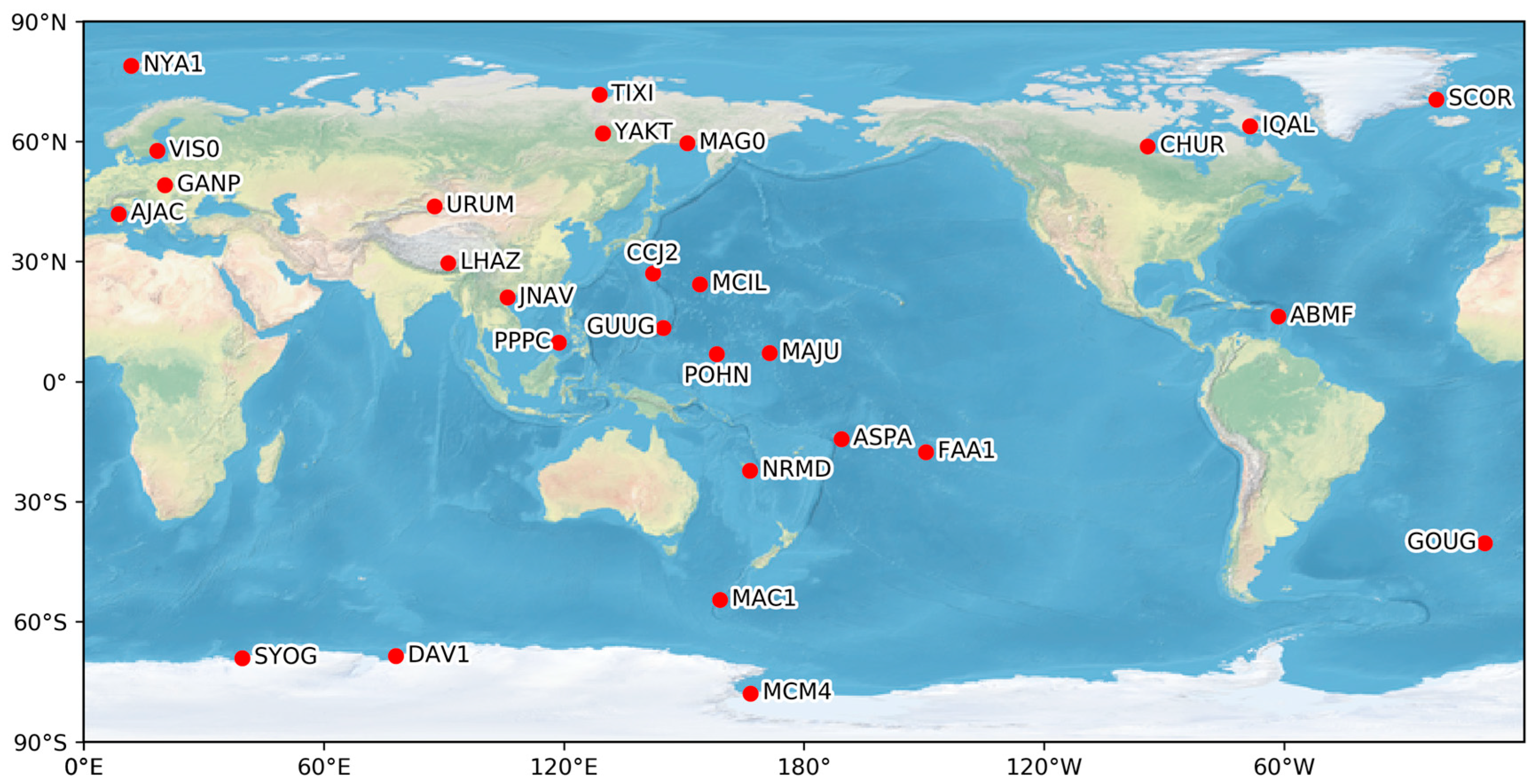
| Stations | ASPA | MAC1 | SYOG | DAV1 | FAA1 | SCOR | MCIL |
| Data Usable | 2048 | 2119 | 2178 | 1834 | 2069 | 2087 | 2089 |
| Rejection Rate (%) | 0.9 | 0.3 | 0 | 0.3 | 3.2 | 0.7 | 4.1 |
| Mean Tropopause (km) | 16.2 | 10.5 | 10.1 | 9.9 | 16 | 10.1 | 16.2 |
| Stations | GANP | GOUG | MCM4 | POHN | ABMF | NYA1 | VIS0 |
| Data Usable | 2149 | 1822 | 1686 | 2036 | 1540 | 1764 | 2000 |
| Rejection Rate (%) | 0 | 1.9 | 0.4 | 1.3 | 2.1 | 0 | 0.2 |
| Mean Tropopause (km) | 12 | 12.4 | 8.9 | 16.4 | 16 | 9.9 | 11 |
| Stations | IQAL | CCJ2 | YAKT | CHUR | URUM | LHAZ | AJAC |
| Data Usable | 1933 | 2032 | 2085 | 2036 | 2140 | 2072 | 2105 |
| Rejection (%) | 0.2 | 6.6 | 4 | 0.3 | 1.3 | 4.6 | 1.2 |
| Mean Tropopause (km) | 9 | 16.1 | 9.8 | 9.9 | 12.6 | 16.3 | 12.9 |
| Stations | PPPC | MAG0 | GUUG | NRMD | MAJU | TIXI | JNAV |
| Data Usable | 1737 | 2134 | 2122 | 2112 | 2110 | 1998 | 2020 |
| Rejection Rate (%) | 6.8 | 1.9 | 0.7 | 3 | 1.6 | 6.2 | 2.1 |
| Mean Tropopause (km) | 16.5 | 9.9 | 16.4 | 16 | 16.4 | 9.5 | 16.4 |
| Data Sources | Stopping Height (km) | Supplementary Atmosphere | Gravity | Curvature of the Earth | Interpolation | Method |
|---|---|---|---|---|---|---|
| Radiosonde | 100 | ISA 1976 | EGM2008 | Gaussian Radius | Pressure: log-linear Vapor Pressure: log-linear Temperature: linear | 2D |
| Elevation Angle | 30° | 25° | 20° | 15° | 10° | 7° | 5° | 3° |
|---|---|---|---|---|---|---|---|---|
| RMS (VMF1) | 0.04 | 0.08 | 0.15 | 0.37 | 1.2 | 3.1 | 7.0 | 20.3 |
| RMS (VMF3) | 0.06 | 0.12 | 0.23 | 0.55 | 1.8 | 4.8 | 11.4 | 36.9 |
| Bias (VMF1) | 0.03 | 0.05 | 0.10 | 0.24 | 0.77 | 2.0 | 4.6 | 13.2 |
| Bias (VMF3) | 0.02 | 0.04 | 0.09 | 0.21 | 0.66 | 1.7 | 3.7 | 10.3 |
| STD (VMF1) | 0.03 | 0.05 | 0.11 | 0.25 | 0.81 | 2.1 | 4.8 | 14.1 |
| STD (VMF3) | 0.05 | 0.10 | 0.19 | 0.46 | 1.5 | 4.1 | 9.9 | 33.0 |
© 2020 by the authors. Licensee MDPI, Basel, Switzerland. This article is an open access article distributed under the terms and conditions of the Creative Commons Attribution (CC BY) license (http://creativecommons.org/licenses/by/4.0/).
Share and Cite
Feng, P.; Li, F.; Yan, J.; Zhang, F.; Barriot, J.-P. Assessment of the Accuracy of the Saastamoinen Model and VMF1/VMF3 Mapping Functions with Respect to Ray-Tracing from Radiosonde Data in the Framework of GNSS Meteorology. Remote Sens. 2020, 12, 3337. https://0-doi-org.brum.beds.ac.uk/10.3390/rs12203337
Feng P, Li F, Yan J, Zhang F, Barriot J-P. Assessment of the Accuracy of the Saastamoinen Model and VMF1/VMF3 Mapping Functions with Respect to Ray-Tracing from Radiosonde Data in the Framework of GNSS Meteorology. Remote Sensing. 2020; 12(20):3337. https://0-doi-org.brum.beds.ac.uk/10.3390/rs12203337
Chicago/Turabian StyleFeng, Peng, Fei Li, Jianguo Yan, Fangzhao Zhang, and Jean-Pierre Barriot. 2020. "Assessment of the Accuracy of the Saastamoinen Model and VMF1/VMF3 Mapping Functions with Respect to Ray-Tracing from Radiosonde Data in the Framework of GNSS Meteorology" Remote Sensing 12, no. 20: 3337. https://0-doi-org.brum.beds.ac.uk/10.3390/rs12203337