Manual-Based Improvement Method for the ASTER Global Water Body Data Base


1
Sensor Information Laboratory Corp., 2-23-36 Shihaugaoka, Tsukubamirai, Ibaraki 300-2359, Japan
2
Institute of Advanced Industrial Science and Technology (AIST), 1-1-1, Higashi, Tsukuba, Ibaraki 302-8564, Japan
3
Department of Aeronautics and Astronautics, University of Tokyo, Tokyo 113-8656, Japan
*
Author to whom correspondence should be addressed.
Remote Sens. 2020, 12(20), 3373; https://0-doi-org.brum.beds.ac.uk/10.3390/rs12203373
Submission received: 2 September 2020
/
Revised: 8 October 2020
/
Accepted: 9 October 2020
/
Published: 15 October 2020
(This article belongs to the Special Issue Remote Sensing Data Sets)
Abstract
:A water body detection technique is an essential part of digital elevation model (DEM) generation to delineate land–water boundaries and to set flattened elevations. The initial tile-based water body data that are created during production of the Advanced Spaceborne Thermal Emission and Reflection radiometer (ASTER) GDEM, as a by-product, are incorporated into ASTER GDEM V3 to improve the quality. At the same time as ASTER GDEM V3, the Global Water Body Data Base (ASTWBD) Version 1 is also released to the public. The ASTWBD generation consists of two parts: separation from land area, and classification into three categories: sea, lake, and river. Sea water bodies have zero elevation. Lake water bodies have flattened elevations. River water bodies have a gradual step-down from upstream to downstream with a step of one meter. The separation process from land area is carried out automatically using an algorithm, except for sea-ice removal, to delineate the real seashore lines in the high latitude areas; almost all of the water bodies are created through this process. The classification process into three categories, i.e., sea, river, and lake, is carried out, and incorporated into ASTER GDEM V3. For inland water bodies, it is not possible to perfectly detect all water bodies using reflectance and spectral index, which are the only available parameters for optical sensors. The only way available to identify the undetected inland water bodies is to manually copy them with visual inspection from the earth’s surface images, like Landsat images. GeoCover2000 images are the main part of the object images. Color–Land ASTER MosaicS (CLAMS) images are used to cover the deficiency of the GeoCover2000 images. This kind of time-consuming, unsophisticated way is inevitable as it is a manual-based method to improve the quality of the ASTWBD. This paper describes the manual-based improvement method; specifically, how deficient water body images are efficiently copied as rasterized images from the earth’s surface images to obtain a more complete global water body data set.
1. Introduction
The Advanced Spaceborne Thermal Emission and Reflection radiometer (ASTER) is an advanced multispectral imaging sensor that was launched on board the Terra spacecraft in December, 1999 [1,2]. ASTER mosaics consist of band 3N as red and band 2 as green. ASTER has an along-track stereoscopic viewing capability in its visible and near-infrared (VNIR) bands at a 15-m spatial resolution with a base-to-height ratio of 0.6. Because of ASTER’s excellent satellite ephemeris and instrument parameters, this along-track stereoscopic viewing capability makes it possible to generate excellent digital elevation model (DEM) data products from ASTER data without referring to ground control points (GCPs) for individual scenes [3,4,5].
Water body detection is an essential part of DEM generation, because image matching is not possible for water bodies. The Global Water Body Data Base (ASTWBD) generation consists of two parts: (1) separation of water bodies from land area, including separation of sea area; and (2) classification of two inland water bodies, i.e., lakes and rivers. The separation process (1) was generated automatically using an algorithm, except for sea-ice removal, to delineate the real seashore lines in the high latitude areas and incorporated into the ASTER GDEM V3 to improve the quality. Almost all the water bodies were created through this process. However, the existence of inland water bodies missed by this automatic process must be kept in mind, as shown later. The separation process (2) was manually carried out with visual inspection (see reference [6] for details). For inland water bodies like lakes and rivers, it is not possible to perfectly detect all water bodies using reflectance and spectral index, which are the only available parameters for optical sensors like ASTER. The only way available to identify the missed inland water bodies is to manually copy them with time-consuming visual inspection from the earth’s surface images, like Landsat images. GeoCover2000 [7] images are a main part of the reference images. GeoCover2000 is used in this paper. Color–Land ASTER MosaicS (CLAMS) [8] images are used to cover the deficiency of the GeoCover images. The original GeoCover data set covers the earth with a 14.25 m spatial resolution and UTM coordinate. The original CLAMS data set covers the earth every 4° latitude by 4° longitude with 0.5 arcsecond posting. Both data sets were converted to the same spatial resolution and coordinates as the ASTER GWBD, i.e., geographic latitude/longitude coordinates with 1 arcsecond posting, and a 1° latitude by 1° longitude tile size. Each ASTER GWBD folder is composed of an attribute file and a DEM file. The attribute file distinguishes a type of water body: a sea water body (Attribute 1), river water body (Attribute 2), and lake water body (Attribute 3). The attribute types are usually depicted with color density slice images in this paper. Attributes 1, 2, and 3 are depicted with blue, red, and green colors, respectively.
The improvement work was accomplished using the support tool that utilizes the “Region of Interest” (ROI) and “Masking” functions of “ENVI” image analysis software by Harris Geospatial Solutions. The support tool “ROI” was used to copy the missed inland water bodies on either object image. Then, the support tool “Masking” was used to import the copied images to the water body image tile, and the improved image tile was saved as a GeoTIFF file.
2. Improvement by GeoCover or CLAMS Images
2.1. Features of the GeoCover and CLAMS Images
GeoCover is a false-color composite image created from orthorectified Landsat Enhanced Thematic Mapper (ETM+) mosaics of band 7 as red, band 4 as green, and band 2 as blue [9,10]. CLAMS is a pseudo-true color composite image created from ASTER mosaics of band 3N as red, band 2 as green, and simulated blue as blue. The simulated blue is used, since ASTER lacks a blue band (see reference [8] for more details about the simulated blue).
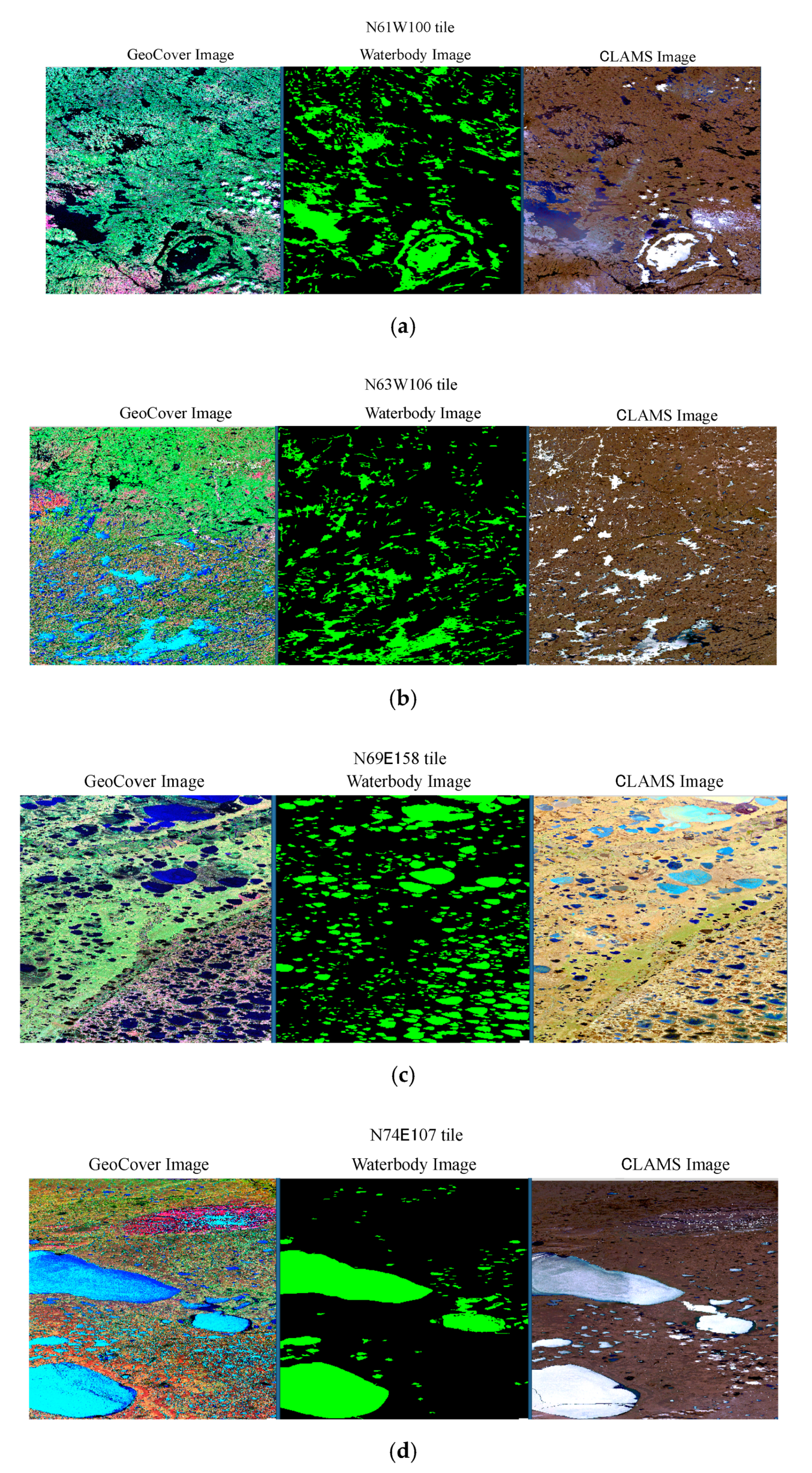
Figure 1 shows the relation between the two reference images and corresponding water body image. The water bodies are shown as green density slice image. In the GeoCover images, water body areas almost accurately correspond to the black and dense-blue color areas. On the other hand, in the CLAMS images, water body areas are widely spreaded from black to white color areas, and then careful judgement will be required.
2.2. How the Improved ASTWBD Was Created
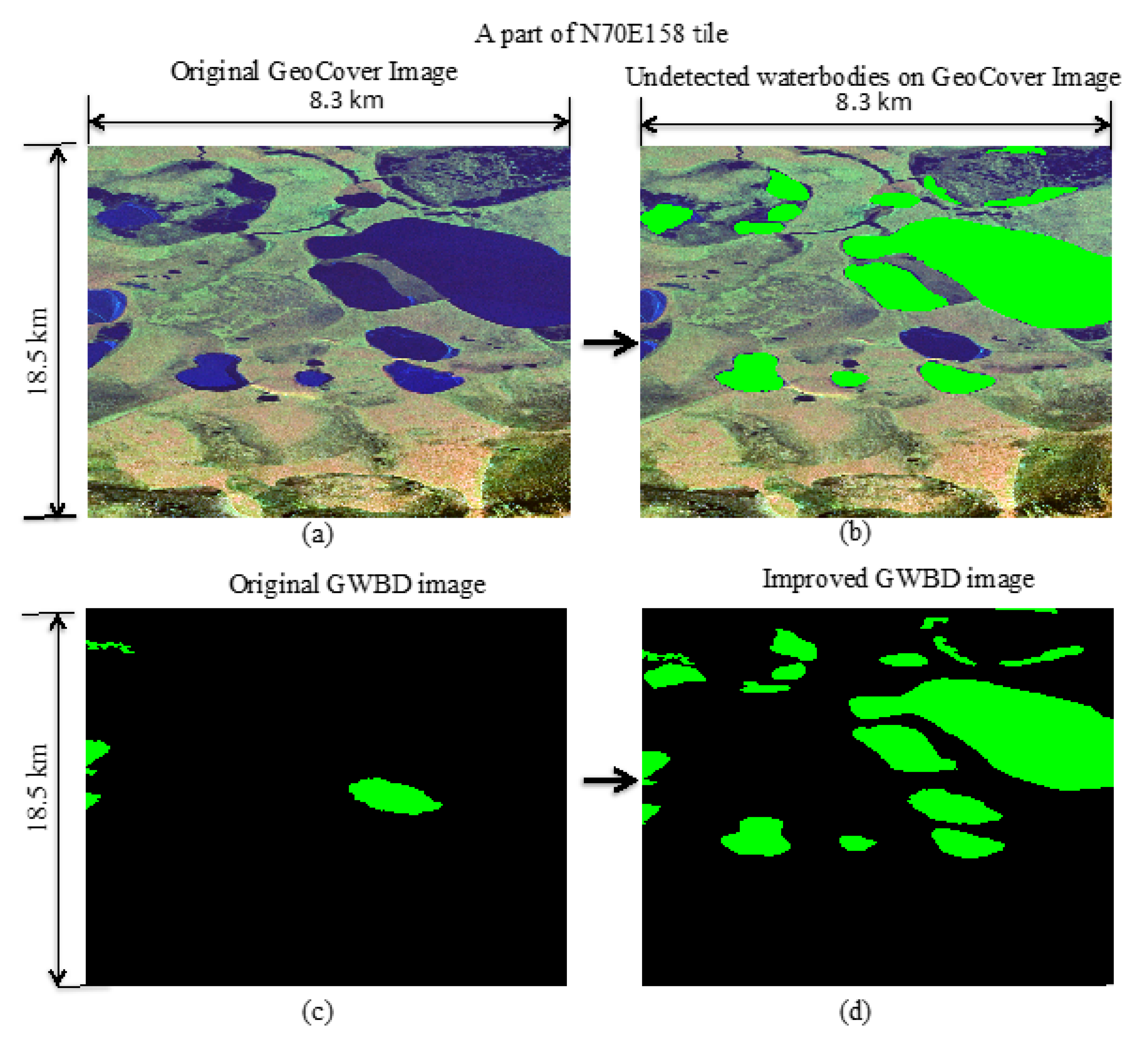
Figure 2 show the water body improvement process using a GeoCover image as the reference image. Each image is a part of the N70E158 tile with an 800-by-600-pixel sub-area that correspond to 8.3 km by 18.5 km, because one arcsecond corresponds to 30.8 m at the equator. The improvement process was carried out as follows:
- (1)
- (2)
- The undetected water body areas are filled in green on the GeoCover image as shown in Figure 2b using the support tool “ROI”. The green color areas correspond to the undetected areas.
- (3)
- The undetected areas on the GeoCover image are imported to the GWBD image and saved as a GeoTIFF file using the support tool “Masking” function.
- (4)
- The final improved GWBD image is shown in Figure 2d.
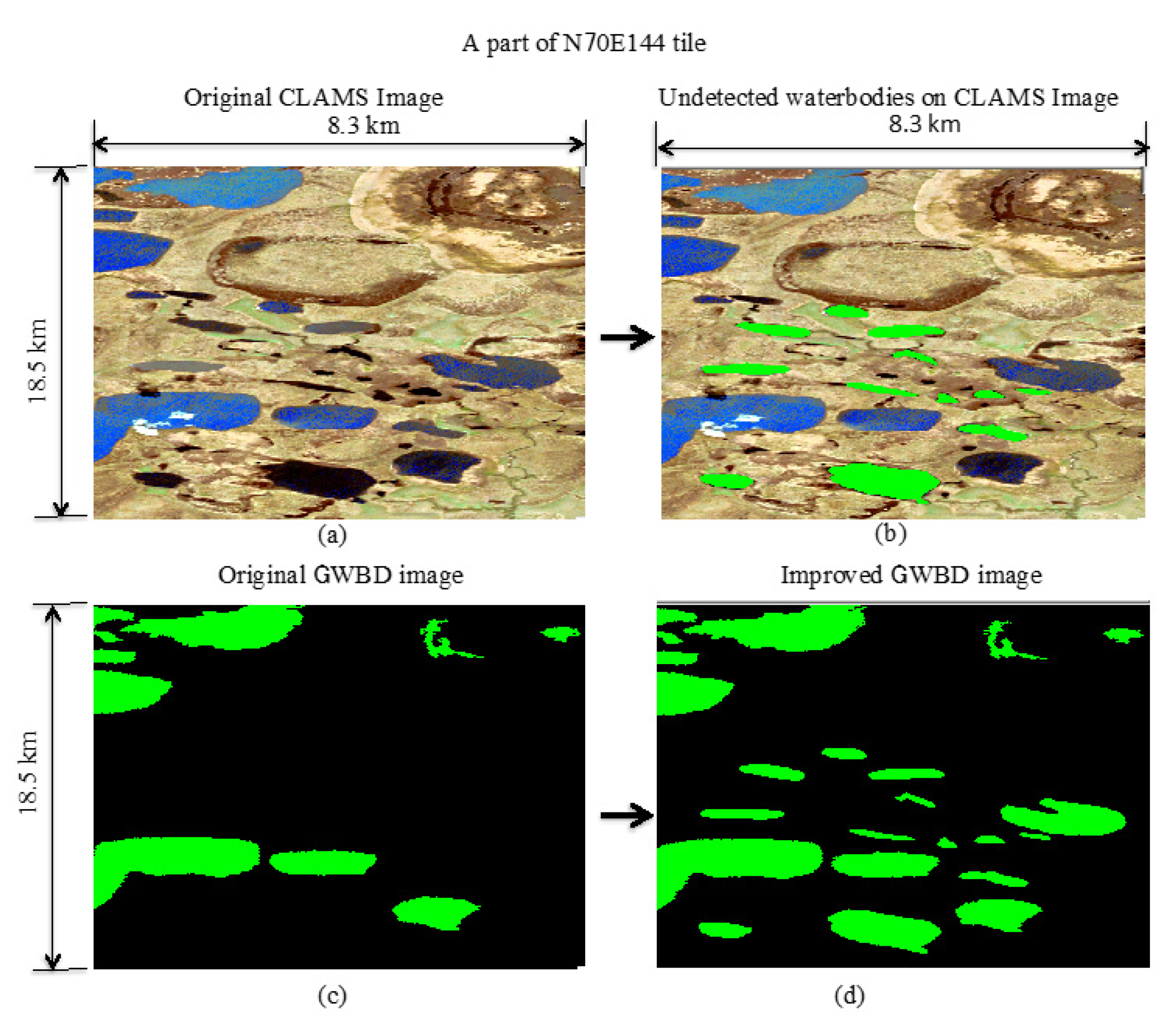
Figure 3 shows the water body improvement process using the CLAMS image as the reference image. The water body improvement process using the CLAMS image is the same as the case of the GeoCover image, as shown above. The GeoCover image is more excellent than the CLAMS image, as shown in the previous section, and so the GeoCover images are used as the main part of the reference images. CLAMS images are used only if the GeoCover image file does not exist.
The water body improvement process is carried out mainly in the area of 60 degrees north and further north latitude, since the Shuttle Radar Topography Mission (SRTM) Water Body Data product (SWBD) [9] is available to make up the undetected water body areas between south 56 degrees and north 60 degrees. South of south 56 degrees areas are not important for inland water bodies because of the frozen Antarctica.
2.3. Typical Examples of Improvements
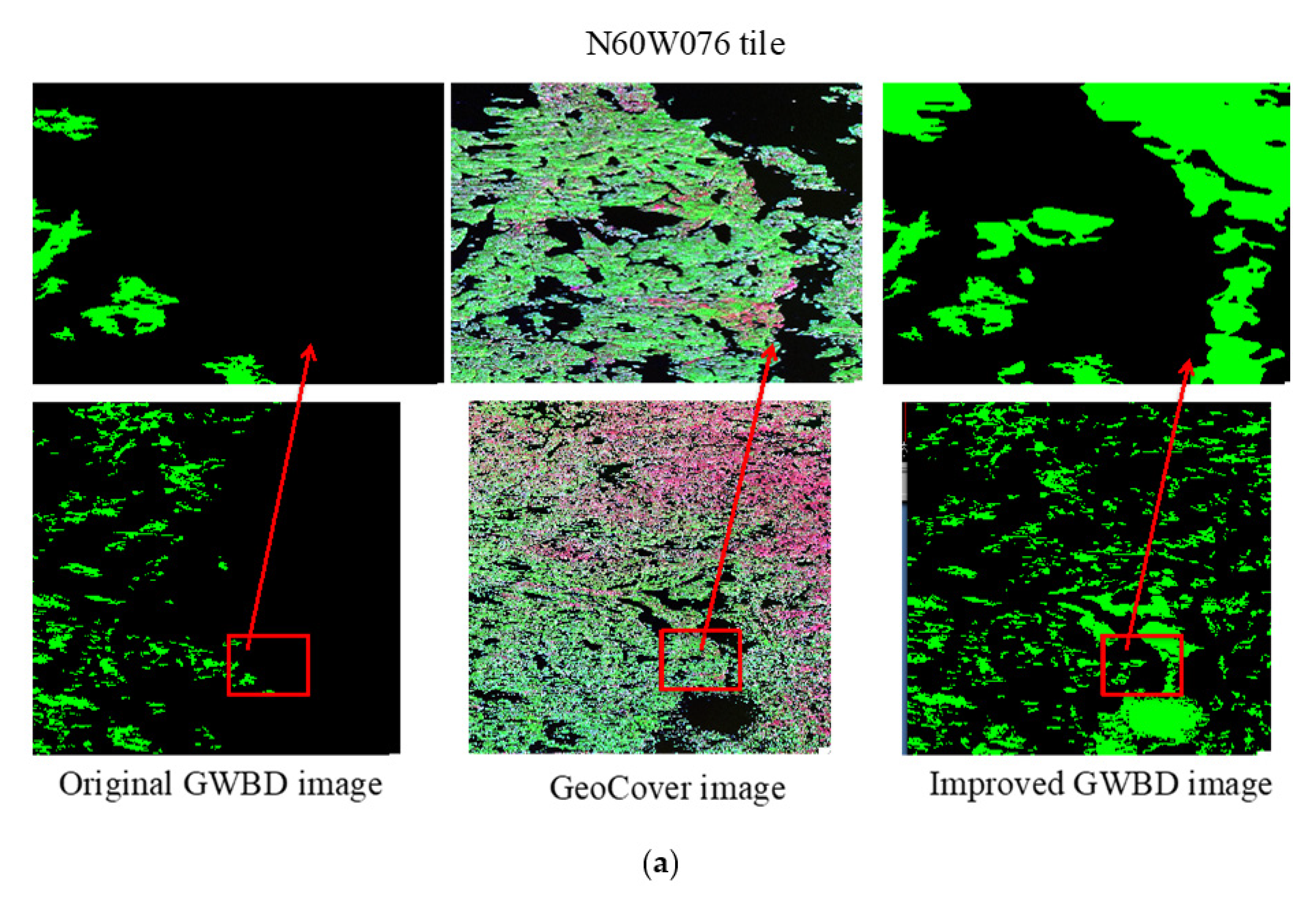
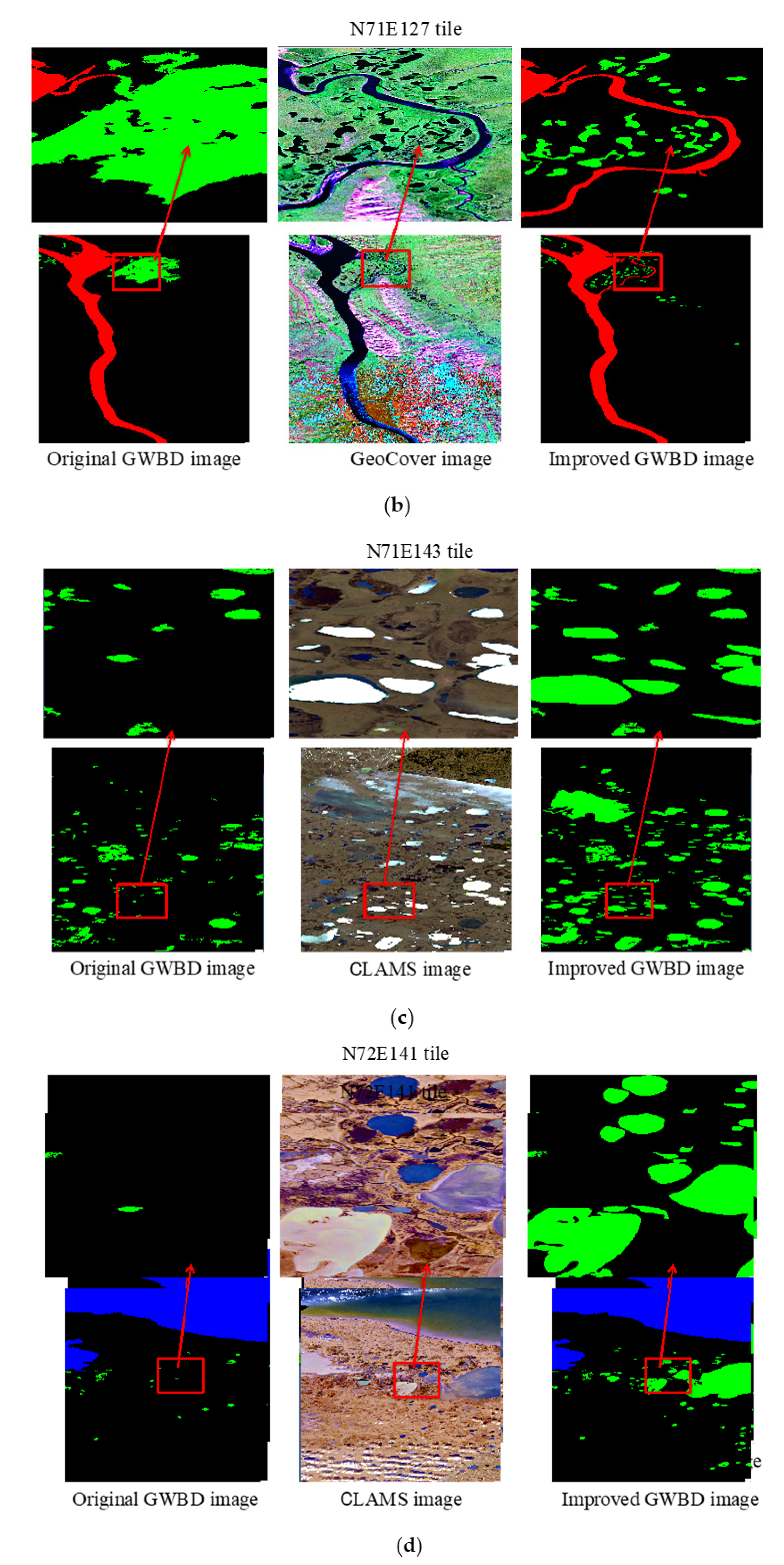
Figure 4 shows four typical examples of the improvement using GeoCover images or CLAMS images. The image tiles with large, increased occupancy ratios were selected as the typical examples. Although the improvements are mainly carried out by GeoCover reference images, it is shown that the CLAMS reference images also play an important role in perfect improvement by covering the deficiencies of the GeoCover images. Figure 4c,d specifically point out that not only small lakes but also large ones are added as water bodies by the CLAMS reference images.
3. Discussion
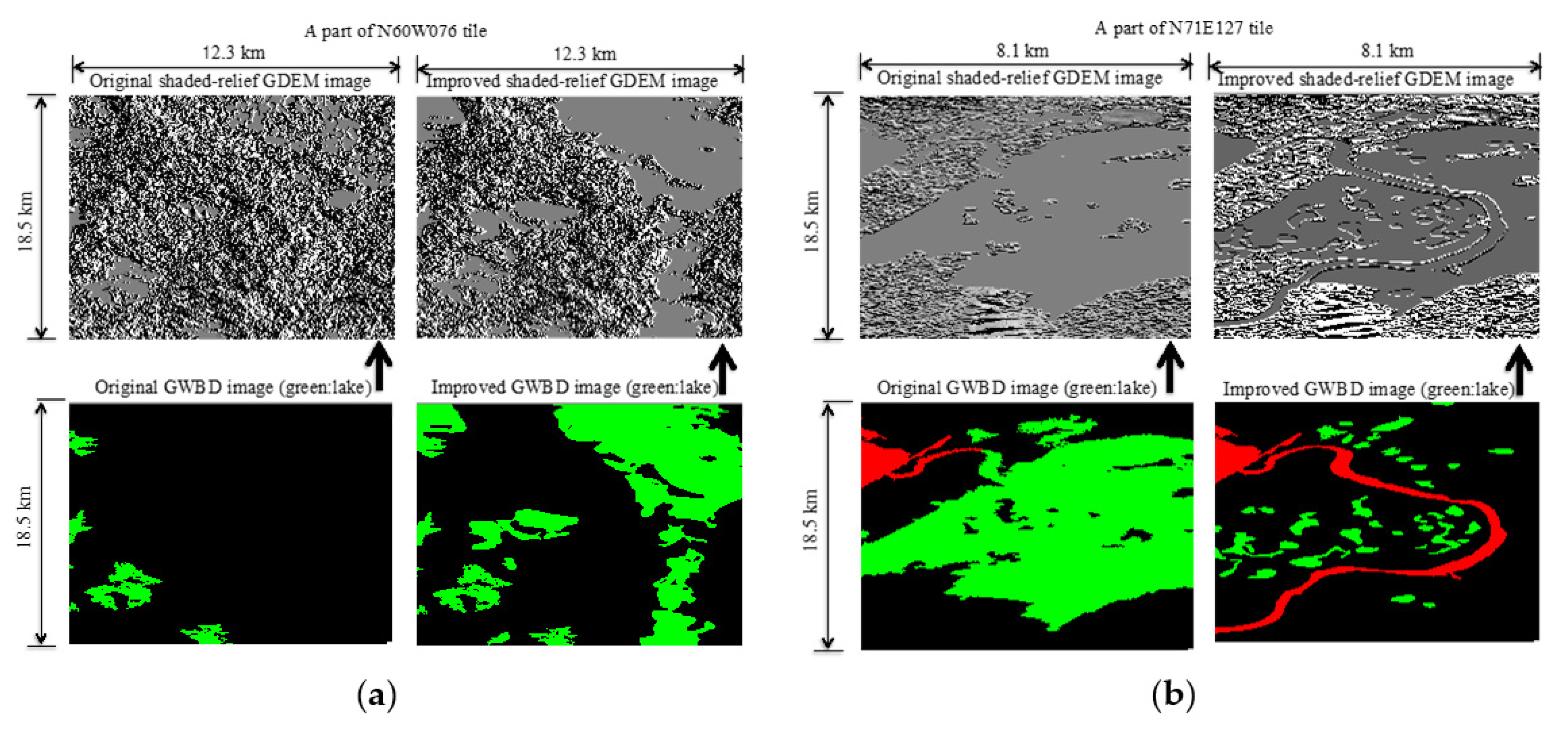
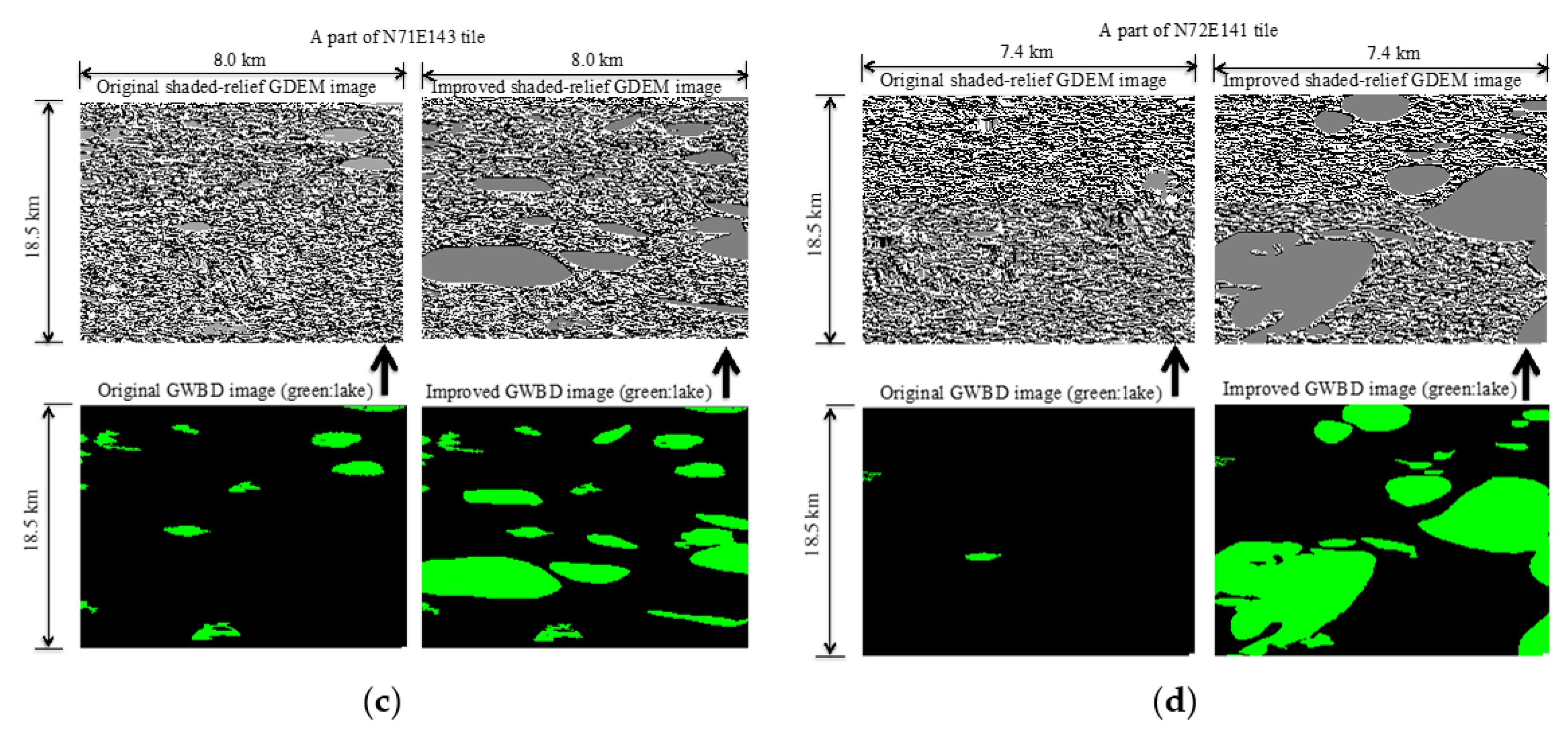
The ASTWBD plays a very important role in the ASTER GDEM generation process, because image matching is not possible for water bodies and is directly linked to ASTER GDEM quality. The special feature of a water body is its flattened elevation value for seas and lakes, and a step-down elevation value from upstream to downstream for rivers. The improved GWBD must be incorporated into the corresponding GDEM image to reflect the improvement effects. Figure 5 shows the effects of the improved GWBD images to the corresponding GDEM images. The image areas are the same as the expanded sub-area of the typical examples shown in Figure 4. Two lower images are the original and improved color density slice GWBD images. A green color denotes a lake water body. The two upper images correspond to the original and improved shaded-relief GDEM images, in which the water bodies are flattened, and clearly show the effect of GWBD improvement on ASTER GDEM quality.
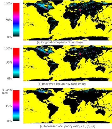
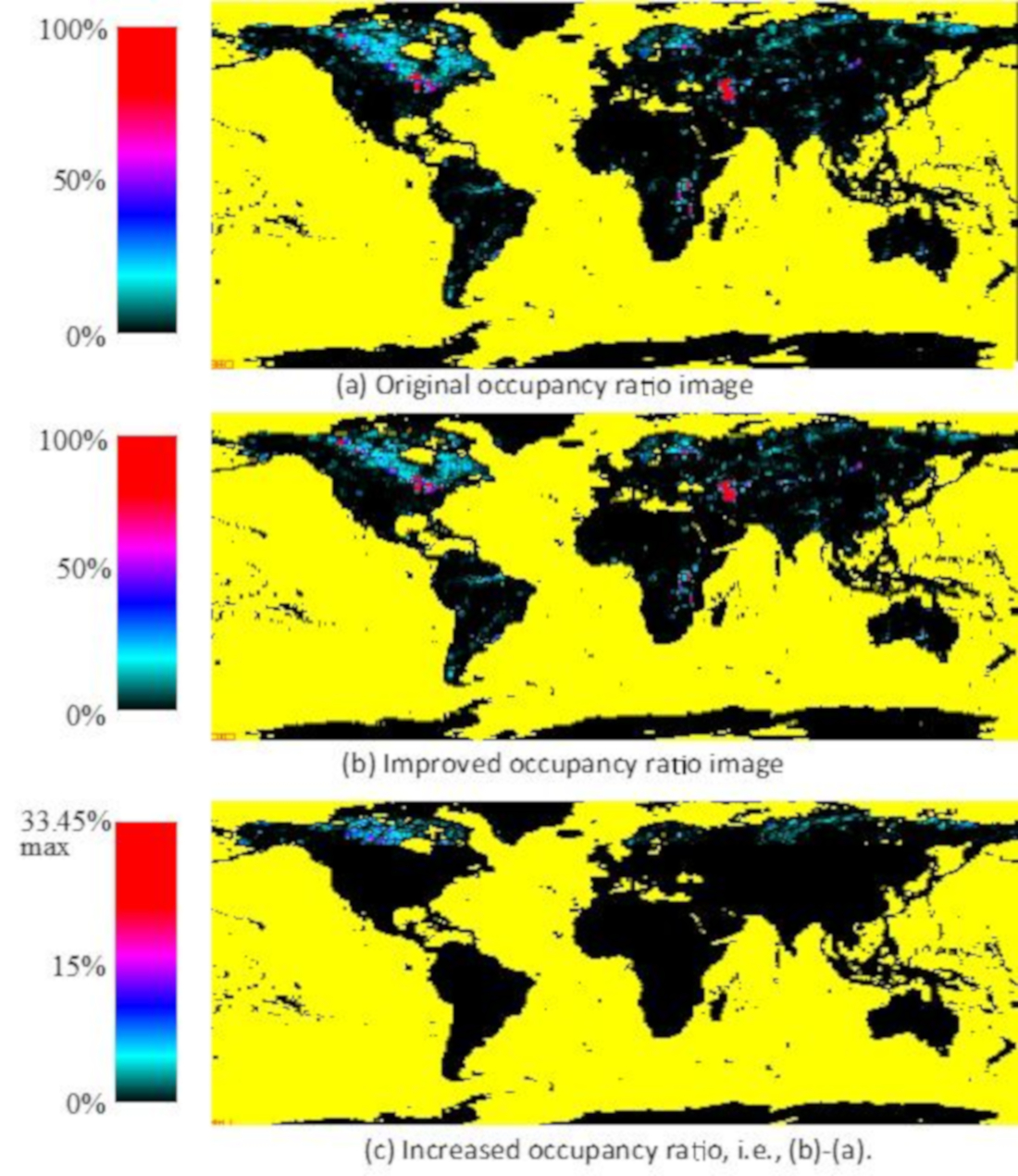
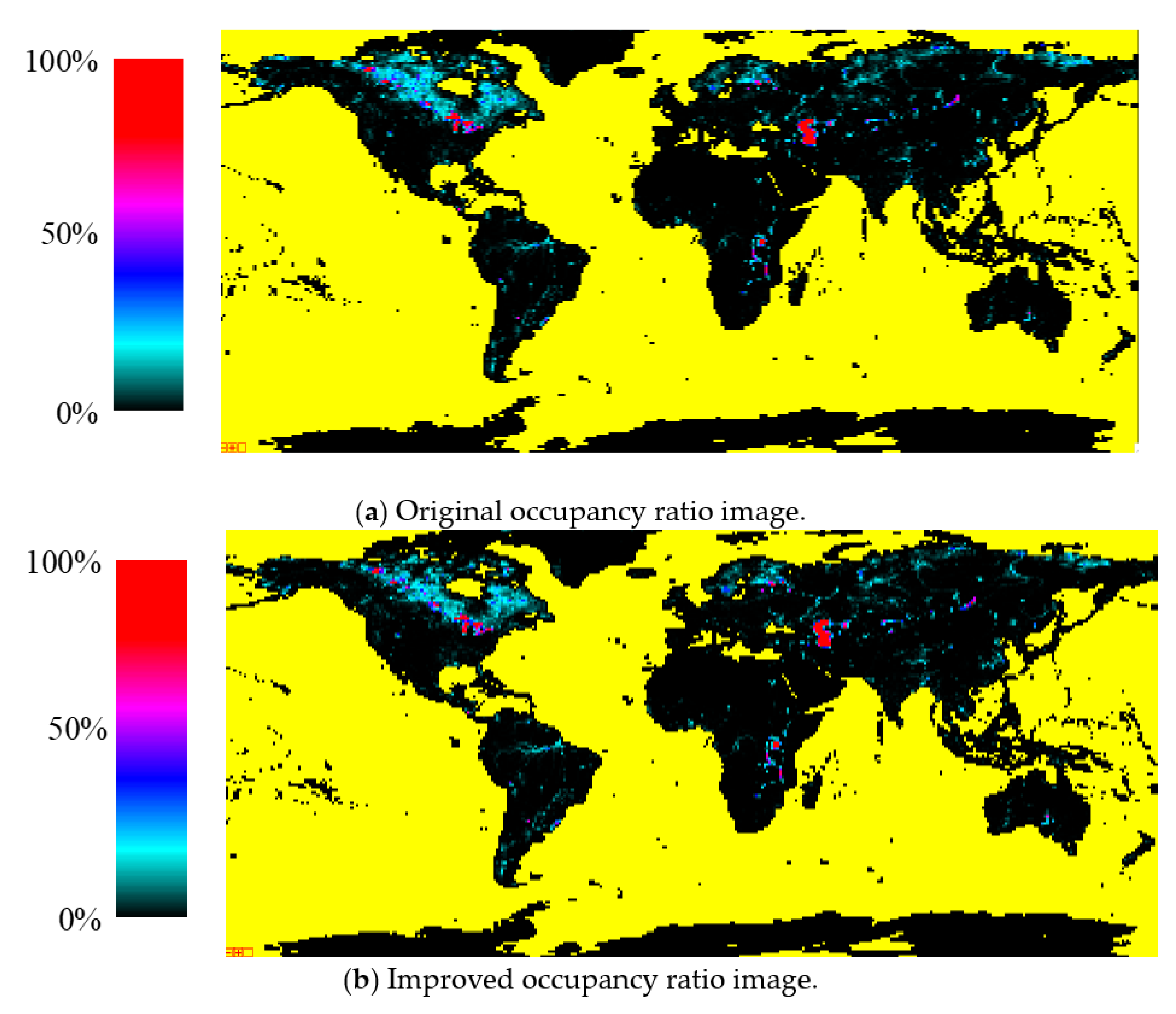
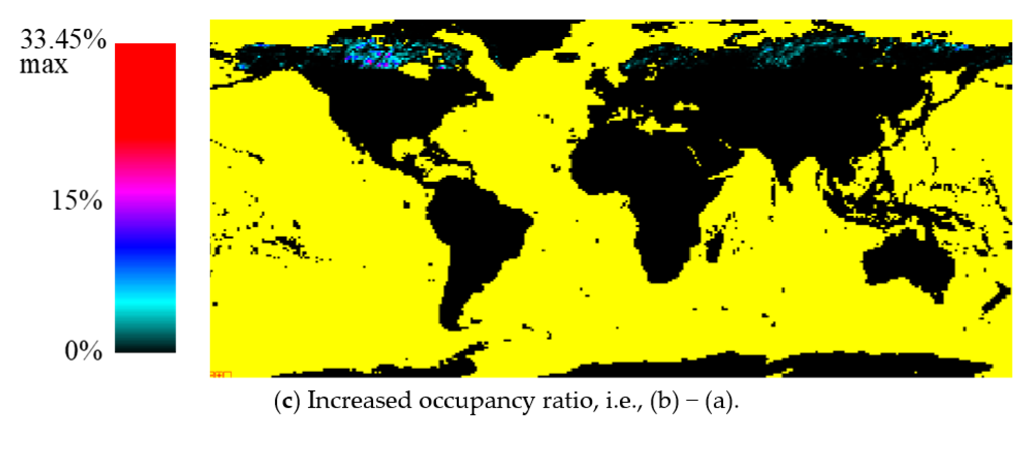
Figure 6 shows the GWBD improvement effects by color density slice occupancy ratio images for inland water bodies on a global scale. Large yellow-color areas denote sea areas. The inland water body means lakes and rivers. In Figure 6a,b, the color density slice images illustrate a red-type color when the occupancy ratios are larger than about 50%, and green- or blue-type colors when the occupancy ratios are smaller than about 50%. On the other hand, in Figure 6c, the color density slice images illustrate a red-type color when the increased occupancy ratios are lager than about 15%, and green- or blue-type colors when the increased occupancy ratios are smaller than about 15%, since the maximum is 33.45%, as shown in Table 2
Figure 6 is very useful to easily understand the various types of global outlines of inland water body distribution conditions. In addition to the global color density slice images of increased occupancy ratio, shown in Figure 6c, and which is main object of this paper, the global color density slice images of the improved occupancy ratio shown in Figure 6b give a complete global water body distribution with a 1° latitude by 1° longitude spatial resolution.
4. Conclusions
Water body detection is an essential part of DEM generation, because image matching is not possible for water bodies. For inland water bodies like lakes and rivers, it is not possible to perfectly detect all water bodies using reflectance and spectral index, which are the only available parameters for optical sensor like ASTER. The only way available to identify the missed inland water bodies is to manually copy them with time-consuming visual inspection from the earth’s surface images, like Landsat images. GeoCover2000 images are a main part of the reference images. CLAMS images are used to cover the deficiency of the GeoCover images. The water body improvement process is carried out mainly in the latitude of 60 degrees north and the further north areas, since the Shuttle Radar Topography Mission (SRTM) Water Body Data product (SWBD) [11] is available to make up undetected water body areas between south 56 degrees and north 60 degrees. South of south 56 degrees areas are not important for inland water bodies because of the frozen Antarctica. The original GWBD corresponds to ASTWBDV001, which was released to the public in August 2019 at the same time as ASTGTMV003 [12]. The ASTWBDV001 data are incorporated into ASTGTMV003. The improved correction was carried out using GeoCover and CLAMS as the reference data.
The improved GWBD almost completely covers all lake-type water bodies with an area greater than 0.2 km2, and can be considered to be the final improvement. Further improvements for ASTER GDEM can be easily carried out by incorporating the improved GWBD into ASTGTMV003.
Author Contributions
Conceptualization, H.F.; methodology, H.F., M.U. and A.I.; investigation, H.F., M.U. and A.I.; writing—original draft preparation, H.F.; writing—review and editing, H.F., M.U. and A.I. All authors have read and agreed to the published version of the manuscript.
Funding
This research received no external funding.
Acknowledgments
We would like to acknowledge Japan Space Systems for supplying the ASTER data. The authors would also like to thank the ASTER Science Team members, specifically Level-1 and DEM Working Group members for their useful discussion. We also would like to acknowledge to National Institute of Advanced Industrial Science and Technology (AIST) for supplying original CLAMS data.
Conflicts of Interest
The authors declare no conflict of interest.
References
- Fujisada, H.; Sakuma, F.; Ono, A.; Kudos, M. Design and preflight performance of ASTER instrument protoflight model. IEEE Trans. Geosci. Remote Sens. 1999, 36, 1152–1160. [Google Scholar] [CrossRef]
- Fujisada, H. ASTER Level-1 data processing algorithm. IEEE Trans. Geosci. Remote Sens. 1998, 36, 1101–1112. [Google Scholar] [CrossRef]
- Fujisada, H.; Bailey, G.B.; Kelly, G.G.; Hara, S.; Abrams, M.J. ASTER DEM performance. IEEE Trans. Geosci. Remote Sens. 2005, 43, 2707–2714. [Google Scholar] [CrossRef]
- Fujisada, H.; Iwasaki, A.; Hara, S. ASTER stereo system performance. Proc. SPIE 2001, 4540, 39–49. [Google Scholar]
- Fujisada, H.; Urai, M.; Iwasaki, A. Advanced methodology for ASTER DEM generation. IEEE Trans. Geosci. Remote Sens. 2011, 49, 5080–5091. [Google Scholar] [CrossRef]
- Fujisada, H.; Urai, M.; Iwasaki, A. Technical methodology for ASTER Global Water Body Data Base. Remote Sens. 2018, 10, 1860. [Google Scholar] [CrossRef] [Green Version]
- GeoCover. Available online: http://www.cr.chiba-u.jp/databases/GeoCover/TM_mosaic.html (accessed on 10 October 2020).
- Gonzalez, L.; Valerie, V.; Yamamoto, H. Global 15-Meter Mosaic from Simulated True-Color ASTER Imagery. Remote Sens. 2019, 11, 441. [Google Scholar] [CrossRef] [Green Version]
- Nelson, G.C.; Robertson, R.D. Comparing the GLC2000 and GeoCover LC land cover datasets for use in economic modelling of land use. Int. J. Remote Sens. 2007, 28, 4243–4266. [Google Scholar] [CrossRef]
- Rajagopalan, R.; Aparajithan, S.; James, S.; Michael, C. Validation of Geometric Accuracy of Global Land Survey (GLS) 2000 Data. Photogrametric Eng. Remote Sens. 2015, 81, 131–141. [Google Scholar]
- NASA JPL. NASA Shuttle Radar Topography Mission Water Body Data Shapefiles & Raster Files; NASA EOSDISL and Processes DAAC: Sioux Falls, SD, USA, 2013. [Google Scholar]
- Abrams, M.; Crippen, R.; Fujisada, H. ASTER Global Digital Elevation Model (GDEM) and ASTER Global Water Body Dataset (ASTWBD). Remote Sens. 2020, 12, 1156. [Google Scholar] [CrossRef] [Green Version]
Figure 1.
Typical examples of GeoCover and CLAMS images to grasp the feature for water bodies. The corresponding water body are shown as green density slice images. Tile size: 1° latitude by 1° longitude: (a) Images of the N61W100 tiles; (b) Images of the N63W106 tiles; (c) Images of the N69E158 tiles; (d) Images of the N74E107 tile.

Figure 2.
The improvement process of undetected water body areas using a GeoCover image as the reference: (a) original GeoCover image; (b) undetected water body areas filled with green on original the GeoCover image; (c) original GWBD image; (d) improved GWBD image. The GWBD images are shown as green density slice images.

Figure 3.
The improvement process of undetected water body areas using a CLAMS image as the reference: (a) original CLAMS image; (b) undetected water body areas filled with green on the original CLAMS image; (c) original GWBD image; (d) improved GWBD image. The GWBD images are shown as green density slice images.

Figure 4.
Four typical examples of improvement using GeoCover images (a,b) or CLAMS images (c,d). For each example, the lower and the upper images show the entire tile images and partially expanded sub-area images with 600 by 400 pixels, respectively. The expanded sub-area in each entire tile image is shown by the rectangular red line. Tile size: 1° latitude by 1° longitude: (a) Images of the N60W076 tiles; (b) Images of the N71E127 tiles; (c) Images of the N71E143 tiles; (d) Images of the N72E141 tiles.


Figure 5.
Effect of improved GWBD to the corresponding GDEM. The two upper images are the original and improved shaded-relief GDEM images. The two lower images are the corresponding original and improved color density slice images. The green color denotes a lake water body, and the red color denotes a river water body: (a) a part of N60W076 tile images; (b) a part of N71E127 tile images; (c) a part of N71E143 tile images; (d) a part of N71E141 tile images.


Figure 6.
Global color density slice images of the improvement effect for the inland water body occupancy ratios. Large yellow-color areas denote sea areas. An inland water body means a lake or river: (a) Original occupancy ratio image; (b) Improved occupancy ratio image; (c) Increased occupancy ratio image.


Table 1.
Detailed quantitative water body occupancy data for the four typical examples shown in Figure 4.
Table 1.
Detailed quantitative water body occupancy data for the four typical examples shown in Figure 4.
| Tile Name | Type of Images | Sea Occupancy (%) | River Occupancy (%) | Lake Occupancy (%) |
|---|---|---|---|---|
| N60W076 | Original image | 0 | 0 | 6.56163 |
| Improved image | 0 | 0 | 18.36819 | |
| N71E127 | Original image | 0 | 8.55893 | 2.52542 |
| Improved image | 0 | 8.81181 | 0.60127 | |
| N71E143 | Original image | 0 | 0 | 4.83586 |
| Improved image | 0 | 0 | 14.03497 | |
| N72E141 | Original image | 22.28395 | 0 | 0.38985 |
| Improved image | 22.28395 | 0 | 6.48122 |
Table 2.
Increased occupancy ratios of the lake-type water bodies in ascending order to the high-ratio areas. The ratios are shown with the corresponding tiles and locations.
Table 2.
Increased occupancy ratios of the lake-type water bodies in ascending order to the high-ratio areas. The ratios are shown with the corresponding tiles and locations.
| Tile Name | Location | Ratio (%) | Tile Name | Location | Ratio (%) | Tile Name | Location | Ratio (%) |
|---|---|---|---|---|---|---|---|---|
| N60E007 | Norway | 5.25127 | N64W095 | Canada | 6.79022 | N68W097 | Canada | 9.95321 |
| N61W098 | Canada | 5.28094 | N68E145 | Russia | 6.81613 | N71W109 | Canada | 10.13983 |
| N71E141 | Russia | 5.33550 | N65W097 | Canada | 6.87522 | N69W105 | Canada | 10.19871 |
| N72E097 | Russia | 5.39406 | N70W112 | Canada | 6.91013 | N61W164 | USA (Alaska) | 10.24639 |
| N60W100 | Canada | 5.40833 | N71W111 | Canada | 6.91214 | N70W111 | Canada | 10.55154 |
| N75E112 | Russia | 5.41753 | N69W125 | Canada | 6.92857 | N65W114 | Canada | 10.56258 |
| N72E142 | Russia | 5.45569 | N63W099 | Canada | 7.04038 | N66W098 | Canada | 10.64937 |
| N71E080 | Russia | 5.46514 | N68W090 | Canada | 7.06019 | N70W157 | USA (Alaska) | 10.67472 |
| N66W105 | Canada | 5.50322 | N71E140 | Russia | 7.16263 | N63W106 | Canada | 10.79045 |
| N70E078 | Russia | 5.52684 | N64W098 | Canada | 7.19305 | N70W154 | USA (Alaska) | 10.94286 |
| N69W098 | Canada | 5.54657 | N61W165 | USA (Alaska) | 7.28413 | N64W114 | Canada | 10.95453 |
| N67W115 | Canada | 5.56222 | N62W108 | Canada | 7.32367 | N63W097 | Canada | 11.10577 |
| N72W108 | Canada | 5.59931 | N63W118 | Canada | 7.38103 | N60W164 | USA (Alaska) | 11.20842 |
| N60W074 | Canada | 5.62596 | N61W099 | Canada | 7.43363 | N70E158 | USA (Alaska) | 11.25973 |
| N63W095 | Canada | 5.63278 | N67W126 | Canada | 7.62890 | N62W102 | Canada | 11.31035 |
| N60W165 | Russia | 5.63698 | N64W115 | Canada | 7.73903 | N62W101 | Canada | 11.33130 |
| N65W105 | Canada | 5.65309 | N71E096 | Russia | 7.76664 | N62W096 | Canada | 11.36850 |
| N61E008 | Norway | 5.67248 | N63W110 | Canada | 7.83731 | N64W108 | N64W108 | 11.47643 |
| N69W104 | Canada | 5.71586 | N62W109 | Canada | 7.95232 | N64W117 | N64W117 | 11.49349 |
| N69E124 | Russia | 5.76290 | N70W105 | Canada | 7.97608 | N68E154 | N68E154 | 11.64781 |
| N65W108 | Canada | 5.85980 | N62W104 | Canada | 8.03119 | N60W076 | N60W076 | 11.80715 |
| N70E079 | Russia | 5.87961 | N69E156 | Russia | 8.08248 | N70W156 | N70W156 | 12.06289 |
| N71E095 | Russia | 5.94174 | N70E159 | Russia | 8.08720 | N65W099 | N65W099 | 12.13787 |
| N61W075 | Canada | 5.94803 | N68W128 | Canada | 8.10427 | N69W113 | N69W113 | 12.33947 |
| N64W093 | Canada | 5.94889 | N63W096 | Canada | 8.13296 | N65W116 | N65W116 | 12.63866 |
| N70W106 | Canada | 5.95411 | N61W096 | Canada | 8.14558 | N63W109 | N63W109 | 12.69144 |
| N70W088 | Canada | 6.00687 | N65W115 | Canada | 8.22398 | N65W113 | N65W113 | 12.88074 |
| N70E150 | Russia | 6.02750 | N64W113 | Canada | 8.25485 | N65W117 | N65W117 | 13.15168 |
| N72E141 | Russia | 6.09137 | N67W105 | Canada | 8.51486 | N66W104 | N66W104 | 13.47813 |
| N63W094 | Canada | 6.09459 | N69E155 | Russia | 8.53566 | N72W107 | N72W107 | 13.65664 |
| N70E153 | Russia | 6.18505 | N72W106 | Canada | 8.75356 | N61W111 | N61W111 | 14.22826 |
| N61W139 | Canada | 6.22052 | N70W110 | Canada | 8.80408 | N61W101 | N61W101 | 14.36880 |
| N64E029 | Finland | 6.25783 | N68E071 | Russia | 8.83583 | N62W095 | N62W095 | 14.62151 |
| N65W104 | Canada | 6.27058 | N68W133 | Canada | 8.96451 | N61W104 | Canada | 14.89520 |
| N71W110 | Canada | 6.35164 | N67W107 | Canada | 8.98649 | N69W112 | Canada | 15.19103 |
| N64W096 | Canada | 6.41225 | N70W155 | USA (Alaska) | 9.00188 | N64W118 | Canada | 15.41963 |
| N61W095 | Canada | 6.44154 | N68E155 | Russia | 9.02434 | N62W100 | Canada | 15.48538 |
| N67W102 | Canada | 6.48683 | N70W153 | USA (Alaska) | 9.09714 | N65W100 | Canada | 15.50255 |
| N63W101 | Canada | 6.52677 | N67W104 | Canada | 9.14772 | N62W103 | Canada | 15.55613 |
| N69W111 | Canada | 6.57954 | N68E070 | Russia | 9.19645 | N66W103 | Canada | 16.04481 |
| N70W113 | Canada | 6.58299 | N71E143 | Russia | 9.19910 | N61W100 | Canada | 16.81194 |
| N64W109 | Canada | 6.59901 | N65W111 | Canada | 9.23940 | N61W103 | Canada | 17.00779 |
| N67W098 | Canada | 6.65046 | N74E107 | Russia | 9.33596 | N63W107 | Canada | 17.57145 |
| N65W098 | Canada | 6.65231 | N69E159 | Russia | 9.40438 | N66W099 | Canada | 17.66327 |
| N70W158 | USA (Alaska) | 6.69218 | N69E158 | Russia | 9.52341 | N60W075 | Canada | 18.45545 |
| N69E146 | USA (Alaska) | 6.70507 | N64W107 | Canada | 9.61353 | N63W108 | Canada | 18.94309 |
| N66W115 | Canada | 6.70820 | N67W106 | Canada | 9.67472 | N62W107 | Canada | 21.11334 |
| N65W157 | USA (Alaska) | 6.74008 | N67W103 | Canada | 9.82968 | N75E142 | Russia | 33.45049 |
Publisher’s Note: MDPI stays neutral with regard to jurisdictional claims in published maps and institutional affiliations. |
© 2020 by the authors. Licensee MDPI, Basel, Switzerland. This article is an open access article distributed under the terms and conditions of the Creative Commons Attribution (CC BY) license (http://creativecommons.org/licenses/by/4.0/).
Share and Cite
MDPI and ACS Style
Fujisada, H.; Urai, M.; Iwasaki, A. Manual-Based Improvement Method for the ASTER Global Water Body Data Base. Remote Sens. 2020, 12, 3373. https://0-doi-org.brum.beds.ac.uk/10.3390/rs12203373
AMA Style
Fujisada H, Urai M, Iwasaki A. Manual-Based Improvement Method for the ASTER Global Water Body Data Base. Remote Sensing. 2020; 12(20):3373. https://0-doi-org.brum.beds.ac.uk/10.3390/rs12203373
Chicago/Turabian StyleFujisada, Hiroyuki, Minoru Urai, and Akira Iwasaki. 2020. "Manual-Based Improvement Method for the ASTER Global Water Body Data Base" Remote Sensing 12, no. 20: 3373. https://0-doi-org.brum.beds.ac.uk/10.3390/rs12203373
Note that from the first issue of 2016, this journal uses article numbers instead of page numbers. See further details here.