Article

CA-Markov Chain Analysis of Seasonal Land Surface Temperature and Land Use Land Cover Change Using Optical Multi-Temporal Satellite Data of Faisalabad, Pakistan

State Key Laboratory of Information Engineering in Surveying, Mapping and Remote Sensing (LIESMARS), Wuhan University, Wuhan 430079, China
*
Author to whom correspondence should be addressed.
Remote Sens. 2020, 12(20), 3402; https://0-doi-org.brum.beds.ac.uk/10.3390/rs12203402
Submission received: 20 September 2020 / Revised: 12 October 2020 / Accepted: 13 October 2020 / Published: 16 October 2020

Abstract

:
Cellular Automata models are used for simulating spatial distributions and Markov Chain models are used for simulating temporal changes. The main aim of this study is to investigate the effect of urban growth on Faisalabad. This research is aimed at predicting seasonal Land-Surface-Temperature (LST) as well as Land-Use and Land-cover (LULC) with a Cellular-Automata-Markov-Chain (CA-Markov-Chain). Landsat 5, 7 and 8 data were used for mapping seasonal LULC and LST distributions during the months of May and November for the years 1990, 1998, 2004, 2008, 2013 and 2018. A CA-Markov-Chain was developed for simulating long-term landscape changes at 10-year time steps from 2018 to 2048. Furthermore, surface temperature during summers and winters were predicted well by Urban Index (UI), a non-vegetation index, demonstrating the highest correlation of R2 = 0.8962 and R2 = 0.9212 with respect to retrieved summer and winter surface temperature. Through the CA-Markov Chain analysis, we can expect that high density and low-density residential areas will grow from 22.23 to 24.52 km2 and from 108.53 to 122.61 km2 in 2018 and 2048, as inferred from the changes occurred from 1990 to 2018. Considering UI as the predictor of seasonal LST, we predicted that the summer and winter temperature 24–28 °C and 14–16 °C and regions would decrease in coverage from 10.75 to 3.14% and from 8.81 to 3.47% between 2018 and 2048, while the summer and winter temperature 35–42 °C and winter 26–32 °C regions will increase in the proportion covered from 12.69 to 24.17% and 6.75–15.15% of city.

Graphical Abstract

1. Introduction

Globally, land use monitoring projects have been integral to international climate and environmental science after the start of the Land Use and Land Cover (LULC) project. Urbanization, marked by replacing natural environments with warm absorbing surfaces and houses, results in high urban temperatures relative to rural and sub urban areas [1]. High temperatures occur in central business districts (CBD) and high density residential (HDR) areas [2]. These kinds of temperature changes may have negative environmental and socio-economic effects on built-up areas, including enlarged consumption of heating and air conditioning thus raising energy prices and pollution-related health threats [3,4]. Nonetheless, due to the substitution of impermeable surfaces and buildings as cities expand their coverage and protection is diminished. The association between future temperature and LULC changes predictions needs to be understood for renewable urbanization and making plans. Surface temperatures and the effect of localized LULC need to be evaluated in order to enhance precision adaptation, prevention, rule design and execution in urban areas.
Several experiments targeted the interaction between LULC trends and LST utilizing remote sensed data without rendering possible predictions [5]. Owing to a mixture of low warm emissivity, weak latent temperature transmission and high heat absorption capacity, this research explained that susceptible surfaces inside urban extents are distinguished by higher temperatures. Conversely, low temperatures are also characteristic of natural landscapes such as wetlands and vegetated areas [6,7]. Research has also looked at natural and long-term historical temperature shifts related to population development [5]. Researchers have used vegetation and urban indices to demonstrate the measurable association between LST and LULC rather than on potential influences from weather trends [8]. For instance [9], describes temperature reduction with the NDVI (Normalized-difference-vegetation-Index) combined with the NDBaI (Normalized-difference-bareness-index) whereas the NDWI (Normalized-difference-wetness-index) is showing rise in temperature with the NDBI (Normalized Difference Built-up Index). The association among LST and variability of indices of LULC is strong, therefore variations in LULC indices such as FVG (Vegetation Fraction) and NDBI have the ability to predict temperature accurately. There is nevertheless a shortage of literature on the usage of LULC indices to predict the potential spatial spread of urban LULC and LST trends.
Despite their success in predicting trends of population development, only one analysis used indices of land cover to estimate projected distribution of soil surface temperature [10]. While [10] the NDVI has been used to estimate residual city normal ecosystems and potential LST values, Normalized difference Vegetation Index is considered to soak at large vegetation fractions, thereby giving a small temperature variation. Previous researches clearly illustrate that Normalized difference Vegetation is a weaker LST predictor than other vegetation and Non-vegetation indices that is, NDBI and ISA (Impervious Surface Areas). In addition [10], single satellite images were used to calculate NDVI to denote the complete season; a technique that is subject to chance, given that a season may differ considerably with a land cover. Therefore, the method has to be changed such as the including seasonal estimates of indices of land cover. In another analysis, calculated LST using a linear regression method on a variety of indices resulting in the Enhanced Build-up and Bareness Index (EBBI), NDBaI, NDBI, NDWI, NDVI, Built-up-Index(BI), Soil Adjusted Vegetation Index (SAVI) and Urban Index (UI) [11]. Thus [10], states that if many variables are included in a linear regression model, the precision of the obtained dependent variable may be affected because of the clatter affected by the collinearity of explanatory factors. Environment predictions are as valuable as they are reliable but hints that a means to estimate LST correctly without errors due to collinearity need to be found first.
To predict changes in LULC and urban expansion, Markov Chain Models have been used [6,12]. For example [9], a Markov Chain analysis for Doha, Qatar, indicated that a 20% rise in built-up areas by 2020 could be expected. Global and local model are widely used to predict temperature excluding urban trend and considering their impact [13,14]. These models are not very fit for understanding regional phenomena as they are at a coarse resolution and therefore need more downscaling [15]. In addition, temperature changes induced by greenhouse gasses are emphasized by global and regional models notwithstanding temperature variations due to the impact of LULC changes. Markov Chain dependent modeling offers an ability to forecast the transition of the environment, offering insights into potential thermal surface characteristics due to vegetation changes [10]. The research is ideal for forecasting variations in temperature at the same spatio-temporal resolution with seasonal variations in land-use land-cover patterns, hence is able to model regional processes such as urban surface dynamics. The Markov Chain model provides tremendous potential for forecasting future LST that needs to be further explored because of earlier achievements in measuring land use land cover shifts relevant effects, usability, flexibility and parsimony. This study is significant for giving direction on how thermal city environments can be projected into future based on the historical patterns of urban development. Much research from various parts of the globe suggest that urbanization contributes to changes in LST but Pakistan still lacks a literature on this issue. The country’s meteorological research have largely used large-scale climate models and in situ meteorological data, focused on precipitation and typically targets agricultural impacts [16,17,18]. Remote sensing-based climate research, however, has remained scarce in the region, particularly at the scale of urban microclimates. The same time, urban development estimates based on remote sensing have concentrated mainly on quantifying recent shifts in LULC over the long term [12].
Many of the communities are growing horizontally and vertically in core markets across the world [19]. Pakistan and specially Faisalabad, do not have a suitable LULC management structure. Recently related urbanization to historical first patterns by means of multi-temporal and spectral Landsat datasets then did not forecast potential developments and their effects on the Faisalabad microclimate. Therefore, to the best of our understanding, predictions of potential population development rates, urban land use designs and its impact on LST based on RS (Remote Sensing) have not yet been produced in Pakistan. Therefore, it is important to predict urban development and consequences for the thermal climate of Pakistani cities with information utilizing remote sensing datasets at medium resolution. This has potential to promote local-level adaptation processes, strengthen the decision related to temperature and boost balanced city development that combines possible micro-climate effects of LULC conversions.
Environmental growth is a troubling problem in developing countries like Pakistan. Pakistan has not made a smooth urban transition due to many factors and one of them is the fact that sustainability has not been a consideration. Thus, research on urbanization, urban expansion and the expansion rate is very important for the economic development of Faisalabad and of great interest to the numerous government authorities, town planners and urban scholars around the globe. Regional policy makers and community planners can profit optimally from the work on sustainable expansion. Such research is particularly necessary in order to decide the borders of the new developments and understand urban sprawl across the Faisalabad region. Rapid urbanization has affected the agricultural land and land use patterns generating problems worldwide. Faisalabad Pakistan is not an exception.
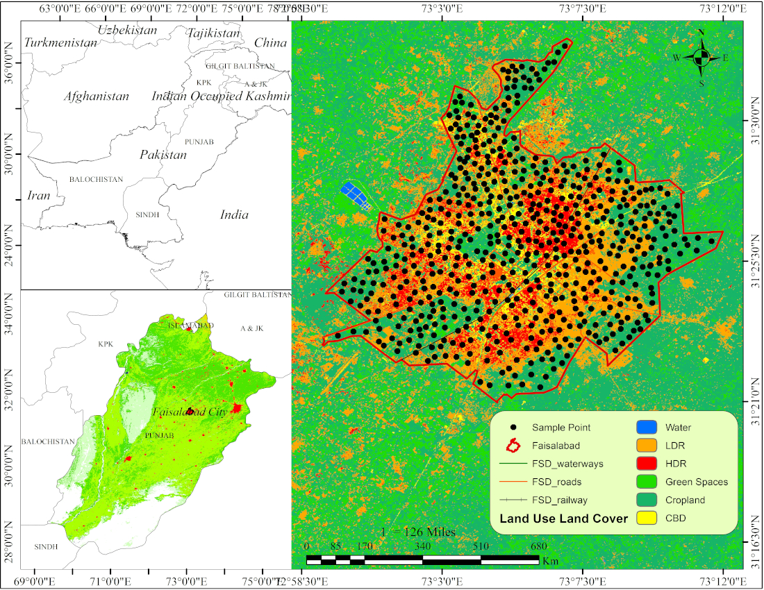
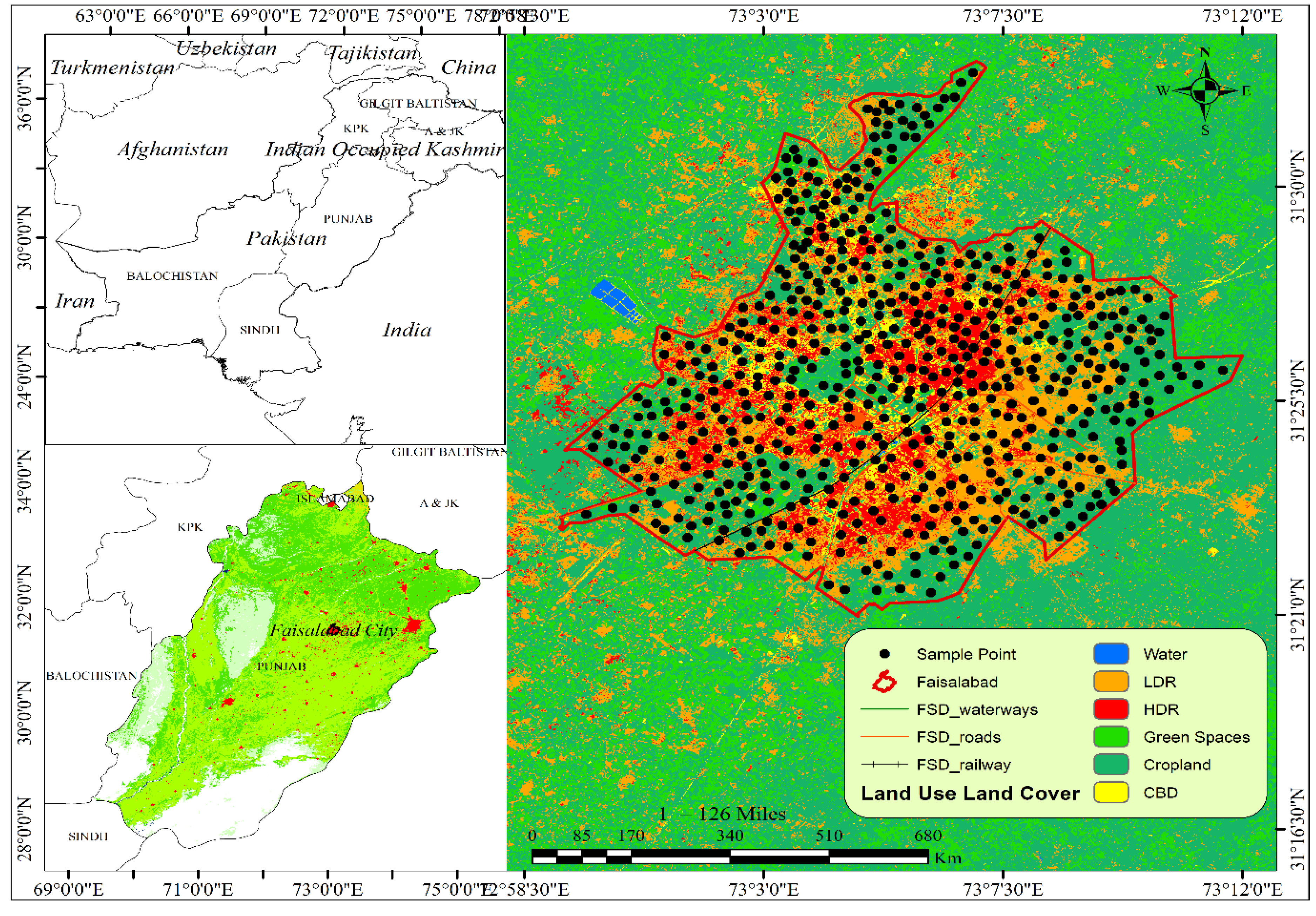
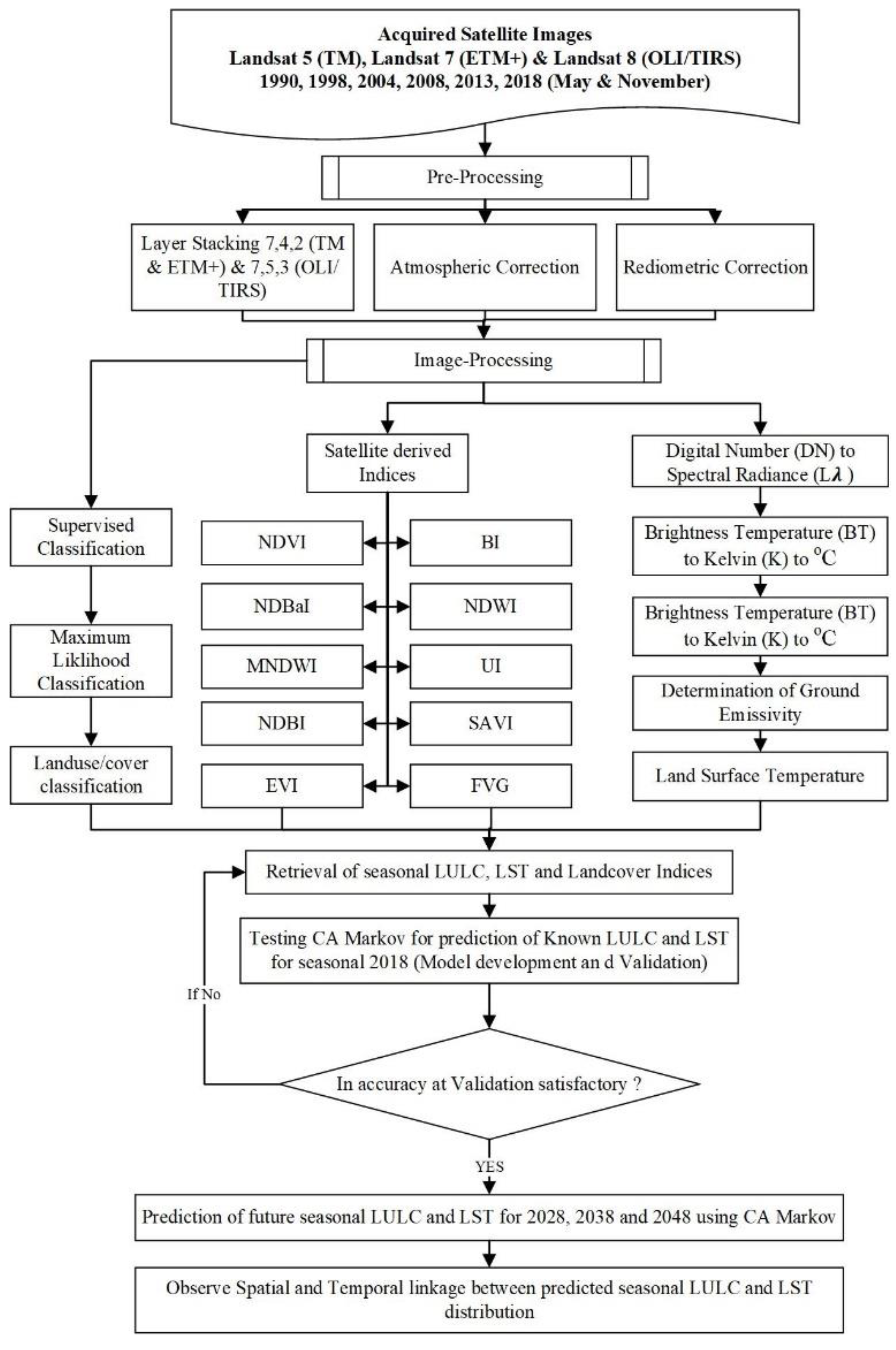
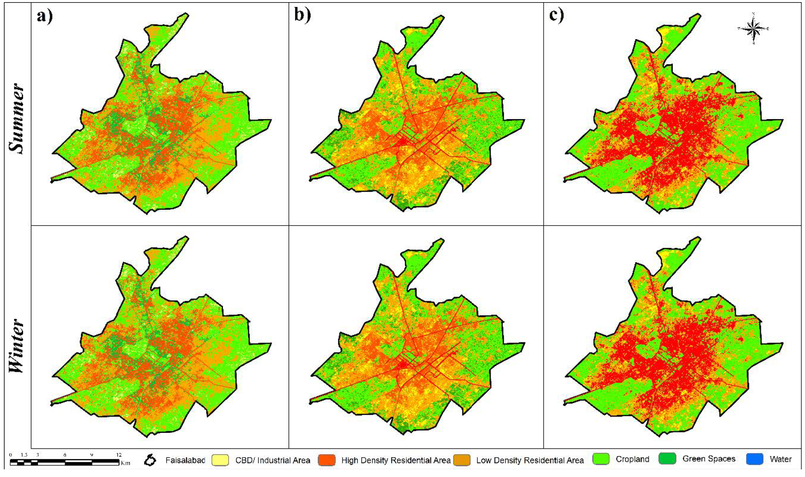
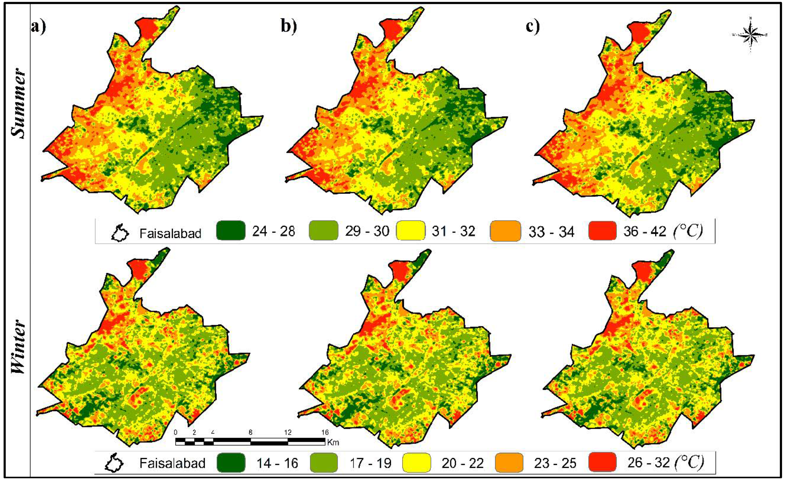
The present research identifies seasonal landcover-indices using Landsat 5, 7 and 8 data representing correlations between seasonal (summer and winter) Land Surface Temperature (LST) and seasonal (summer and winter) Land Use Land Cover (LULC) changes in Faisalabad, Punjab, Pakistan from 1990 to 2018. The study also identified the specific indices most suited for prediction of the seasonal distribution of Land Use Land Cover and LST using the CA-Markov-Chain. A further objective was to use seasonal images of summer (May) and winter (November) in land cover indices instead of single season as used in earlier studies when modeling seasonal patterns of land cover as input in the Cellular Automata Markov model.

2. Materials and Methods

2.1. Study Area

This research was conducted in the industrial city of Faisalabad, Pakistan. It lies from 31°25′15″ N to 73°5′21″ E (Figure 1). The plain fields of Faisalabad are mostly situated on the upper east side of the Punjab, with a height of 604 feet (184 m) above sea level. The city appropriately spreads a territory of roughly 52,142 acres of land while the district approximately covers 1,443,703 acres. In 1901 the population of Faisalabad was 9171 persons, that growing to 70,000 in 1941 and 179,000 in 1951 after partition due to the migration of Muslim refugees. After ten years, the figure had reached 425,000. According to the 1998 census the population had increased to about 2.009 million, exceeding 3.56 million in 2018. The lower Chenab trench is the fundamental water source infrastructure responsible for irrigation across 80% of the cultivated fields. Faisalabad rests on alluvial loess soils with calcareous characteristics, rendering the region extremely productive. The Chenab river flows in the north-west for around 30 km while the Ravi river flows in the south-east at around 40 km from the area. The temperature highs in the city range from 45 °C in summer to 15 °C in winter. The daily mean maximum and minimum summer temperatures are 39 °C and 27 °C. This drops to about 17 °C and 6 °C in winter [20,21].

2.2. Data Acquisition and Image Processing

Landsat 5 Thematic Mapper (TM), 7 Enhanced Thematic Mapper Plus (ETM+) and 8 Operational Land Imager/Thermal Infrared Sensor (OLI/TIRS) medium resolution images were used to calculate LULC and LST. Images of Faisalabad with path/rows of 149/38 were obtained from United States Geological Survey-Center for Earth Resources Observation and Science (USGS-EROS) (http://earthexplorer.usgs.gov/) for two seasons, summer (May) and winter (November) in1990, 1998, 2004, 2008, 2013 and 2018. All these images had less than 10% cloud cover (Table 1). Landsat data were selected because they are easy to access and widely used for classification in LULC and LST analysis. We used cloud free images for analysis as illustrated in Table 1 and Table 2. For atmospheric correction we used the Fast Line-of - Sight Atmospheric Analysis of Spectral Hypercubes (FLAASH) module in ENVI v_5.4 (Harris Geospatial Solutions, Inc., USA) [22]. Image pre-processing began with layer stacking to create a multispectral image after combining the necessary bands. The images were also calibrated for noise removal [23]. This technique was important to help provide any useful details about the data at the time of data collection, that is, sensor size, sun elevation and atmospheric state. Scanning lines from 2004 and 2008 were eliminated from Landsat 7 (ETM+) in ENVI v_5.4 using Landsat gapfills.sav extension on each band using a triangular approach. After scanning the lines from each band, both bands were opened in Arc Map 10.6 and the bands exported at the same resolution (spatial and radiometric) as Landsat 7 (ETM+). All the maps were geometrically modified using 45 Ground-Control-Points (GCP), toposheet (1:50,000) and aerial-imagery, all GCP obtained on satellite images at the intersection of invariant features and roads. The city boundary was obtained from Urban Unit Remote Sensing and Geographic Information System (GIS) Lab.
Seasonal satellite images from 1990, 2004 and 2018 were used to develop the model and evaluate the accuracy for predicting land surface variations whereas data from 1990, 1998, 2004, 2008, 2013 and 2018 (Table 1) were used to construct real seasonal predictions. To check the performance of this model, the 10-years interval of satellite images (1998, 2008 and 2018) was changed. Table 1 illustrate that beginning of the summer (all of images from May) and winter (all images from November) season in 1990, 1998, 2004, 2008, 2013 and 2018. One satellite image from each season was used annually to allow calculation of surface temperature and vegetation & non-vegetation indices for the prediction of seasonal LULC and seasonal LST distributions. The impact of randomness was eliminated by using seasonal averages.

2.3. Land Use Land Cover Classification (LULC) Accuracy Assessment and Mapping

LULC maps for the years 1990, 1998, 2004, 2008, 2013 and 2018 were obtained from Landsat 5, 7 and 8 reflective bands of 30 m using monitored Support-Vector-Machine (SVM) algorithms. Six LULC categories that is, Central Business District/Industrial Area (CBD/I. Area), High-Density Residential Area (HDR Area), Low-Density Residential Area (LDR Area), Green-Spaces (G. Spaces), Croplands (Crops) and Water/Wetlands (Water) were obtained from every image as indicated in Table 2 [24].
The Support-Vector-Machine algorithm was selected because it does not interfere with the likelihood function and has minimum training data requirements. The Support-Vector-Machine algorithm has established itself in land use landcover classification relative to other classifiers such as the Parallelepiped, Minimum-Distance, Maximum-Likelihood-Classifier (MLC), Artificial-Neural-Network (ANN) and Mahalanobis-Distance classifiers [25,26]. Field observations support training and accuracy assessment in supervised classification. A field survey conducted between March and June 2018 obtained 25 representative GPS points per class except water class. Based on the points were divided into preparation (80%) and testing (20%). Samples of points using a region of interest instead of points increase the reliability of validation results. Specialist expertise and ancillary Land Use Land cover data from previous studies, aerial photos and toposheets were used to establish ground-truth regions for evaluation of classification accuracy. For determining the precision of LULC classifications, the kappa (K) coefficient and overall-accuracy (OA) were used. Post classification [27] variations for every landcover-class from 1990 to 2018 were utilized to measure urban development trends in Faisalabad.

2.4. Calculation of Vegetation Indices and Urban Indices

Table 3 lists the vegetation and urban indices that were tested for their potential to predict seasonal LST. Table 3 contains of Urban-Indices (UI) calculated using the digital numbers (DN) of specified bands and indices of vegetation, calculated by reflecting the specified bands [11]. As mentioned multiple indices were evaluated for predicting LST.

2.5. LST Estimation Using Landsat Data

For each year, land surface temperatures were obtained from the Landsat TM and ETM+ (B6) and Landsat OLI/TIRS (B10) thermal bands developed on the dates shown in Table 1. To limit the seasonal influences, the satellite images were taken in the month of May and November. There are two thermal bands (10 and 11) in the Landsat 8 (OLI/TIRS) imagery but only band 10 was used for LST estimation [38]. Land surface temperature recovery includes the transformation of digital numbers ( D N ) to radiances ( L λ ), the measurement of radiance brightness-temperatures ( T B ) and the adjustment of emissivity in order to extract surface temperatures from brightness maps [39].
In this research Landsat TM & ETM+ and OLI/TIRS thermal band data from1990, 1998, 2004, 2008, 2013 and 2018 were used to retrieve seasonal (summer and winter) land surface temperatures. Using the Reflectance Toolbox an extension applied to ArcMap 10.6 (ESRI, USA) Equation(1) was used to transform digital numbers ( D N ) to radiances ( L λ ) [23,40]. The tool extracts metadata files from parameters and applies them to the matching thermal data. Brightness temperature was obtained from thermal radiance by means of Equation (2) which is the Landsat channel basic approximation of Planck’s blackbody temperature [8,41].
For LST estimation the following series of equations has been used. For each pixel, digital number ( D N ) was converted into the radiance ( L λ ) as follows:
L λ = ( L m a x λ L m i n λ Q C A L m a x L Q C A L m i n ) + L m i n λ ,
where L m a x λ is maximum radiance values, L m i n λ is the minimum radiance values, Q C A L m a x the maximum quantized calibrated pixel value (corresponding to L m a x λ in DN (255)), Q C A L m i n is the minimum quantized calibrated pixel value (corresponding to L m i n λ in DN (01)) respectively; and the metadata of the Landsat images provide their values. Secondly, the L λ values were converted into brightness temperature T B as in:
T B = ( K 2 l n ( K 1 L λ + 1 ) ) 273.5 ,
where K 1 and K 2 are constant value and available from the United States Geological Survey (see Table 4) [42]. From every thermal band, we retrieved from spectral radiance and black body the pixel-based land surface emissivity map (ε), as developed [43] and also applied recently [44]. Ultimately, real LST was obtained using Equation (3) after emissivity correction (ε) was applied to the brightness temperature [42].
T S = T B [ 1 + [ λ T B p ] l n ε ] .
The λ sign define wavelength of emitted radiance ( λ = 11.5 µm), while p is equivalent to 1.438 × 10 2 m k . Using this method, LST was obtained from all the satellite images mentioned in Table 1. The land surface temperature illustrates long term temperature fluctuations in the season and training models in order to predict LST. The average earth surface temperature for 1990, 1998, 2004, 2008, 2013 and 2018 was determined by thermal data for the dates seen in Table 1. This was undertaken to test whether the LST were still rising in reaction to urbanization and to determine if potential development could be expected.

2.6. Prediction of Temperature by Selecting Variables

A strong correlation between the surface temperature and predictor variables, with no collinearity among the variables is required in seasonal land surface temperature calculation. Degree of correlation with seasonal LST were assessed by indices appearing in Table 3. The seasonal indices having maximum correlation with seasonal LST were chosen to predict seasonal LST using a linear regression model. The association between such variables was also tested to exclude strongly clustered predictors that may trigger collinearity-related errors. Indices strongly correlated with seasonal LST and weakly with each other were used to develop a multi-variate linear model. To evaluate the model’s efficiency, we used it to predict the 2018 observed seasonal LST. Mean Absolute Percentage Error (MAPE) -Equation (4) [29] was used to quantify the accuracy.
M A P E % = 1 N i = 1 N ( | T p r e d i c t e d T o b s e r v e d T o b s e r v e d | ) i × 100 ,
where T p r e d i c t e d is the model surface temperature and T o b s e r v e d is the real ith pixel of LST reported from Landsat info. The absolute mean percentage is an accuracy prediction metric that represents error in terms of percentage. The model’s precision in temperature prediction was measured using the Nash-Sutcliff performance, Root Mean Square Error (RMS), Mean Bias Error and Agreement-Index. The model was applied after accuracy evaluation to predict the seasonal distribution of LST at 10-years intervals for the period from 2028 to 2048. An interval of ten years was selected because the analysis showed noteworthy variations at parallel stages in the time.

2.7. Modeling of LULC Changes for 2028, 2038 and 2048

Numerous predictive models have been used to represent the seasonal LULC [45]. The flowchart in Figure 2 describes the technique for predicting potential seasonal LULC and LST distribution from remote sensing data collection utilizing CA-Markov-chain analysis [5,46]. Simulation tests for 2004 were contrasted with an actual map for 2004. In this analysis, the 2018 state simulation was performed for validation purposes in order to equate the expected with the real distribution of LST. Section 2.7.1 and Section 2.7.2 expand the specifics of the outlined measures.

2.7.1. Use of CA-Markov Analysis to Predict Urban Expansion in Faisalabad

IDRISI Selva 17.0 (Clark Labs, USA) is an optimized, certified image processing and Geographical Information Program that offers approximately 300 modules for interactive spatial information analysis and display [47]. The platform provides environmental control, policy support, risk identification, simulation and surface characterization methods. A Markov Chain, is a tool to evaluate adjustments in land use among cycles by a sequence of values that depend on present state [6,48]. The Markov model allows it possible for the structure to progress from the original state i to j over a time period T [9]. The Markov Chain was selected because of its capabilities in predicting time changes LULC [6,45]. In addition, the Markov Chain can predict complex system variations [45]. For other simulations, then, the Markov Chain outputs are used as inputs to generate maps of potential allocation of land usage. Because of its simplicity and parsimony, the Cellular Automata (CA) was nominated to map the spatial dispersal to predicted urban expansion and effect on LST [6,49]. The 2018, 2028, 2038 and 2048 LULC distribution prediction were made using the coupled Cellular-Automata and Markov-Chain the (CA-Markov chain) models in the IDRISI software Selva v_17.0 [1,50,51,52]. The changes probabilities maps acquired from the Markov Chain analysis were used as inputs to the Cellular Automata (CA) model that maps the future land use landcover distributions. Hence the synthesis of Markov Chain and Cellular Automata exposed spatio-temporal shifts in land use and land cover. We checked their ability to forecast future LULC trends in a dynamic urban environment and applied a CA Markov Chain to make real predictions. We used seasonal LULC shifts between 1990 and 2004 to predict seasonal LULC distribution for 2018 and seasonal LULC transformations between 1998 and 2008 to predict seasonal LULC distributions for 2018 and contrasted both sets of results. The predicted land use landcover was compared with the shape obtained in 2018 using the Support Vector Machine classifications. The forecast performance for 2018 was measured using the Kappa-Agreement-Index (KIA), which measures the degree of consensus between two maps (1990 and 2004, 1998 and 2008) of the same case [51]. Thus, the KIA was used to evaluate performance of the CA-Markov in predictive LULC changes by comparing the LULC map form supervised SVM classification with the modeled map for 2018. After assessing the CA-Markov-Chain model precision, we used LULC seasonal patterns of 1990, 2018 subsequently for predicting seasonal landscape for 2028, 2038 and 2048.

2.7.2. Prediction of LST Distribution in Faisalabad Using CA Markov Chain Study of Land Cover Indices

The Urban Index (UI) was chosen as the best predictor variable of LST distribution as defined in Section 2.6. To avoid restricting the arbitrariness related with one image, an average UI was determined in each of the years 1990, 2004 and 2018 using images collected in May and November (Table 1). The 1990 and 2004 average UI was inserted into the Markov-Chain model to produce changes likelihood matrices used in the CA model to map the potential state of the index for 2018. Likewise, in CA-Markov chain results the mean urban indices for 1990 and 2018 was used to estimate UI status in 2028, 2038 and 2048. For 2018, 2028, 2038 and 2048, UI prediction were converted into distribution of LST by using linear regression function (Section 3.4). As the classes were predicted by CA-Markov Analysis, UI maps were re-classified into a model to predict summer temperature classes of 24–28 °C, 29–30 °C, 31–32 °C, 33–34 °C and 36–42 °C and winter classes of 14–16 °C, 17–19 °C, 20–22 °C, 23–25 °C and 26–32 °C. The groups were selected solely to allow a comparison of summer and winter LST distributions in different years to map classes of surface temperatures observed in 1990 and 2018 with the same ranges. Summer and winter LST predictions for Faisalabad city for 2028, 2038. and 2048 were the outcomes of this step.

2.7.3. Statistical Significance of Analyzing Urban Expansion and LST

We checked the statistical significance of predicted seasonal variations in land use land cover and dispersal of LST between 2018 and 2048. The test was applied to coded land use land cover values and to temperature level values derived from 600 points. For each period the LST groups were coded 1–5, whereas the LULC levels were coded 1–6 based on Markov analysis criteria and performance. We used the Shapiro-Wilk statistic to initially test for regularity [47]. Meanwhile, the variations in land use landcover and LST were checked for relevance using the Mann Whitney statistic [29,53]. We checked the Ha hypothesis about the spatial distributions of seasonal LULC and LST is distinct from the alternative Hb hypothesis: in 2018 and 2048 the pairs of LULC and LST were not same [24].

3. Results

3.1. LULC and Seasonal Changes Observed from 1990 to 2018

Table 5 presents variations in seasonal LULC distribution recorded at high accuracy using the SVM Algorithm between 1990 and 2018. As shown, the accumulation of built-up areas in the central region and extended from 1990 to 2018. Table 5 describes summer and winter season in two sections. Urban expansion could be investigated from landcover maps and in summer season, CBD/I. area, HDR and LDR was increased from 1.53 km2 (0.76%) to 6.35 km2(3.14%), 8.77 km2 (4.35%) to 22.23 km2 (11.28%) and 57.53 km2 (28.51%) to 108.34 km2 (53.70%) (Table 5). Meanwhile, G. Spaces, Crops and water area was decreased from 18.70 km2 (9.27%) to 16.40 km2 (8.13%), 114.31 km2 (56.65%) to 47.92 km2 (23.75%) and 0.93 km2 (0.46%) to 0.52 km2 (0.26%) respectively (Table 5).The Table 5 winter part indicate that the CBD/I. area, HDR and LDR area was increased from 1.53 km2 (0.76%) to 6.35 km2 (3.14%), 8.77 km2 (4.35%) to 22.23 km2 (11.28%) and 57.53 km2 (28.51%) to 108.34 km2 (53.70%) and G. Spaces, Crops and water area decreased from 13.25 km2 (6.57%) to 6.74 km2 (3.34%), 114.49 km2 (56.74%) to 45.77 km2 (22.68%) and 1.38 km2 (0.68%) to 0.84 km2 (0.41%) respectively. In the summer season, OA and K were 88.83% and 0.86, 87.23% and 0.88, 84.56% and 0.86, 85.20% and 0.79, 79.32% and 0.71 and 88.2% and 0.81 and in winter season 84.78% and 0.83, 85.39% and 0.78, 85.36% and 0.81, 85.99% and 0.83, 85.32% and 0.65 and 75.35% and 0.69 for the years 1990, 1998, 2004, 2008, 2013 and 2018, respectively. Table 5 displays the LULC transformations as the city expanded between 1990 and 2018. Built-up areas expanded in Faisalabad from 1990 to 2018, at the disbursement of G. Spaces and Crops (Table 2). For instance, built-up areas expanded exponentially, while Crops and G. Spaces declined from 1990 through 2018.

3.2. Seasonal Temperature Changes Observed Satellite Based from 1990 to 2018

Seasonal LST increased between 1990 and 2018 in response to urban development in Faisalabad. as Figure 3 reveals that in 1990, as compared to later years, during the summer season, the region was dominantly covered by temperatures in the range 24–28°C and 29–30°C. The 36–42 °C group was dominant in 2018 while lower categories of surface temperature remained in some parts of the main area of the study region. In the central region with CBD / I. area and HDR area, larger temperature increases were found than in the outer areas with crops and G. Spaces.
While LST warms significantly over period, temperatures less than 28 °C are normal in low density cropland, G. Space and suburban identified areas. However, higher surface temperatures occurred in the CBD/I. Area even during the winter period (Figure 4), such as in 1990 and 1998. Most of the CBD/I. area and HDR suburban zones fell in the range 26–32 °C during the winter season.
A summary of the seasonal changes in LST observed in Faisalabad between 1990 and 2018 is given in Table 6. When the city expanded between the seasons the proportion of summer LST in the categories 29–30 °C decreased by around 37% and 17–19 °C categories decreased by 22% in the winter season due to development of CBD I. area and HDR. During the same period, high LST coverage increased nearly 12% in the summer season (35–42 °C) and nearly 6% in the winter season (26–32 °C), suggesting a strong ground warming bias in Faisalabad.

3.3. Variables Selection: Correlation between Temperature and Urban Indices

Table 7 indicates a strong correlation between the summer, vegetation and non-vegetation indices and the land surface temperature. The BI, NDWI, MNDWI (Modified Normalized Difference Water Index), UI and NDBI coefficients are at magnitudes greater than 0.5. The other indices showed a lower temperature correlation; for example, the NDBaI had the poorest surface temperature correlation. The other indices displayed negative temperature association; in the summer season, for instance, the EVI (Enhanced Vegetation Index), FVG, NDVI and SAVI had a negative correlation. The Urban Indices had the strongest strong negative correlation with summer FVG (R2 = −0.7133) but a strong positive correlation with summer temperature (R2 = 0.9467).
Table 8 indicates a strong positive correlation among LST and BI, UI and NDBI as suggested by coefficients of correlation exceeding 0.5. The other indices showed lowest temperature correlation; for instance, the MNDWI and NDBaI had the weakest correlation and NDVI, NDWI, SAVI, EVI and FVG had negative surface temperature correlation. Urban Indices had the strongest winter temperature correlation (R2 = 0.9212) and also had a strong negative correlation to winter FVG (R2 = −0.2353). As the highest correlation was with LST. The Urban Indices have been discovered to be the excellent predictor of urban LST in comparison to different indices.

3.4. Extraction of LST from Urban Index

Figure 5 illustrates regression model of the urban indices for forecasting seasonal LST. The relationship between surface temperature and urban indices for summer and winter season was too strong that is, summer (R2 = 0.89) and winter (R2 = 0.92). Therefore, in both seasons, land surface temperature and urban indices had increased and did not affect their relationship due to saturation that disturb indices like NDVI, as the UI continuous to rise with unbounded temperature.

Use of Urban Indices in Accuracy Assessment of Temperature Retrievals

The linear regression model was evaluated in May and November 2018 on individual Landsat results. These strongly resembled the observed temperature patterns (see Figure 6). Tsat define is the satellite observed temperature and Tmod define modeled derived temperature. The seasonal temperature obtained from the UI was contrasted with that recovered directly collected from Landsat 8’s thermal data depending on 600 sampled points throughout the area of study (see Figure 1).

3.5. Prediction of LST and LULC (Summer and Winter) for 2028, 2038 and 2048

3.5.1. Accuracy Assessment of Cellular Automata Markov Chain LULC (Summer and Winter) for 2028, 2038 and 2048

Visual examination displayed association between the distribution of land use and land cover assessed using the SVM classifier and the distribution of land use and land cover of 2018 projected using the CA-Markov (Figure 7). The model replicates the spatio-temporal dispersal of seasonal forms of LULC as defined by the support vector machine, driven by in-situ-observations. The average KIA predicted using CA-Markov between the summer and winter LULC and the dispersal calculated by using SVM classifier were 0.88 and 0.85 (Table 9). In the summer, the agreement between the green spaces and the weakest (KIA = 0.78) among the water classes in the two maps was strongest (KIA = 0.89). In the winter, the agreement between the high- and low-density residential area and the weakest (KIA = 0.79) was among the cropland classes in the two maps was strongest (KIA = 0.86).

3.5.2. Prediction of Seasonal LULC Dispersal in Faisalabad

Figure 8 illustrates that, in 2028, 2038 and 2048, the CA-Markov-Chain model predicted expansion in HDR and LDR areas associated with water and G. Spaces. Thus, if trends found between 1990 and 2018 remain constant, built-up areas might invade parks.
According to Table 10, residential areas are projected to rise from their present extent through 2048. CBD/I. areas, for example, are projected to expand from 6.89 to 7.92 km2 between 2028 and 2048. HDR areas are projected to expand from 22.92 to 24.52 km2. LDR areas are projected to expand from 113.92 to 122.61 km2. As the region expands, crops will likely decline in area from 41.60 to 33.51 km2 while G. Spaces fields will decrease from 15.86 to 12.82 km2 at the same period. In the winter season, CBD/I. area, HDR and LDR area would be increased from 6.89 to 7.92 km2, from 229.2 to 24.52 km2 and from 2028 to 2048 to 113.92 km2 to 122.61 km2. G. spaces and crops regions probably will reduce in size from 12.80 to 9.04 km2 and 44.30 to 37.11 km2. Thus, according to the model projections and expectations, potential development may primarily be marked by growth of HDR at the decrease of water, g. spaces and crops regions.

3.5.3. Seasonal Temperature Changes Predicted in Faisalabad before 2048

Figure 9 illustrate the temperature increasing trend from 2028 to 2048. The model further explained summer and winter LST changes between 2028 and 2048 due to increase in built up area. The extent of high surface temperature (>35 °C) in summer (Figure 9a–c), was projected to rise at the cost of lower temperature classes. Thus, eastern and southern areas having LDR areas were colder than CBD/I. area, HDR areas in central and north western in all the predictions that is, 2028, 2038 and 2048. Most of the area of low temperature (24–28 °C and 29–30 °C) transferred to the high temperature category area (33–34 °C and 35–42 °C). Most of the areas, particularly in the north western and central area, could shift towards high temperature (>35 °C) whereas the extent of low temperature classes (24–28 °C and 29–30 °C) may reduce (Table 11).
The model predicted that the temperature ranges from 24 to 28 °C might decrease coverage 13.52–6.32 km2 whereas the temperature ranges in the 36–42 °C category are expected to rise from 37.87 to 48.67 km2 from 2028 to 2048. The high temperature category (>26 °C) likely rise at the expense of lower temperature categories as suggested by the winter Figure 9 winter (a–c). Most of the temperature increase will occur in the CBD/I. area, HDR and LDR areas. Most of the area of low temperature (14–16 °C and 17–19 °C) will become high category areas (23–25 °C and 26–32 °C). Many areas particularly in the center and north western part could shift towards higher temperatures (>26 °C) whereas the extent of lower temperature (14–16 °C and 17–19 °C) might decrease as shown in Table 11. The model predicted that temperature range of 14–16 °C and 17–19 °C might decrease in coverage from 13.99 to 6.79 km2 and from 71.63 to 60.83km2 while the temperature range in the 23–25 °C and 26–32 °C category is expected to rise from 35.83 to 46.63km2 and from 18.87 to 29.67 km2 between 2028 and 2048.
Figure 9. Predicted temperature distribution for Faisalabad city in (a) 2028, (b) 2038 and (c) 2048.
Remotesensing 12 03402 g009

4. Discussion

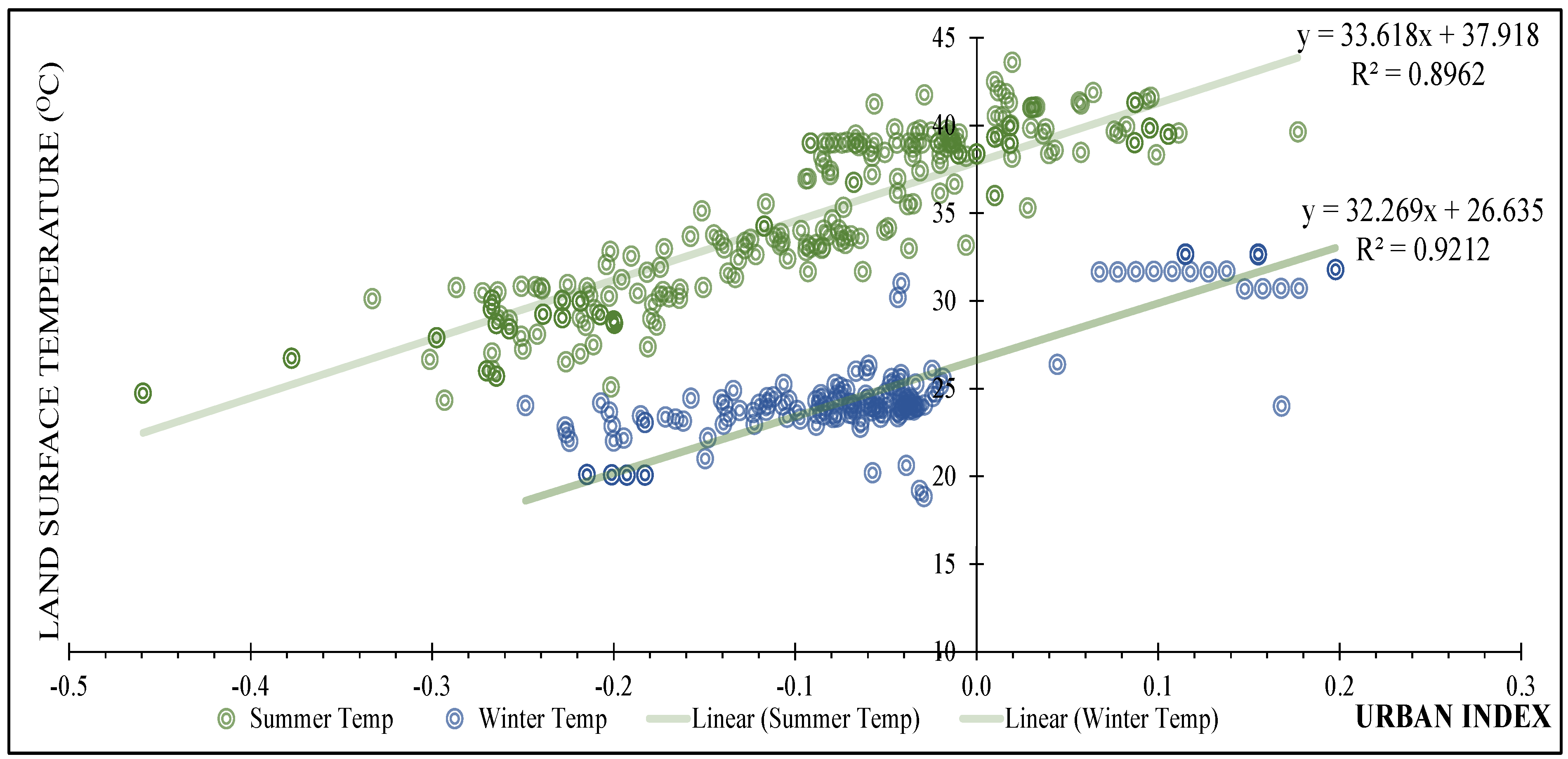
In this research and Cellular Automata Markov Chain models were developed for prediction of seasonal land use landcover and seasonal LST in Faisalabad, Pakistan. The predictive ability of a number of indices for landcover were assessed in relation spatio-temporal temperature. Among a number of indices such as NDBI, FVG and NDVI, the UI was considered as the prior index for predicting LST distribution. Urban expansion and spatiotemporal temperature were predicted by using linear regression model. When the projected variables are not related to each other, it is appropriate to use multiple linear regression [10,
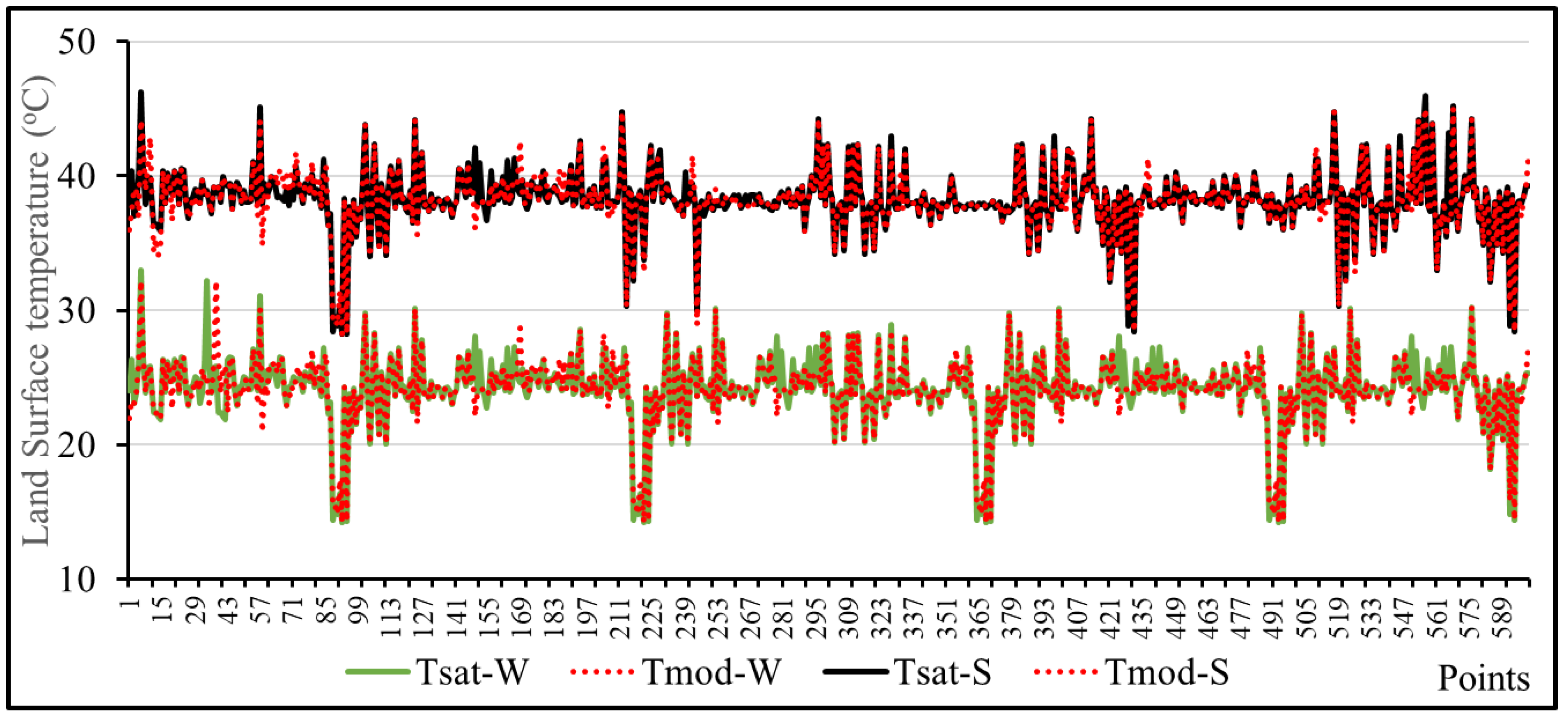
54]. Through a diagnosis analysis, all predictors were correlated hence we found that UI provided the most robust temperature explanation. We used the UI as a reference for urbanization and its projected spread to model possible types of LST spread. The model projected temperature with an absolute average error of 1.85 °C by comparing LST computed from thermal band and linear model using UI. UI‘s success in projecting urban development based heating can be clarified by recent research that have found it to be closely associated with a number of urban expansion metrics [55]. For example [55], observed UI increased with building density and decreased with NDVI in Tokyo Bay.
While the association between temperature and UI has not been verified in earlier research, the strong predictive strength found in this analysis is attributed to elevated temperatures in areas with HDR and less vegetation. [54] also reported strong urban indices in water-intensive and residential parts of Sri Lanka and Colombo. Research have also revealed that the use of water and household energy rises with the intensity of urban weather, thus the strong association between UI and LST [
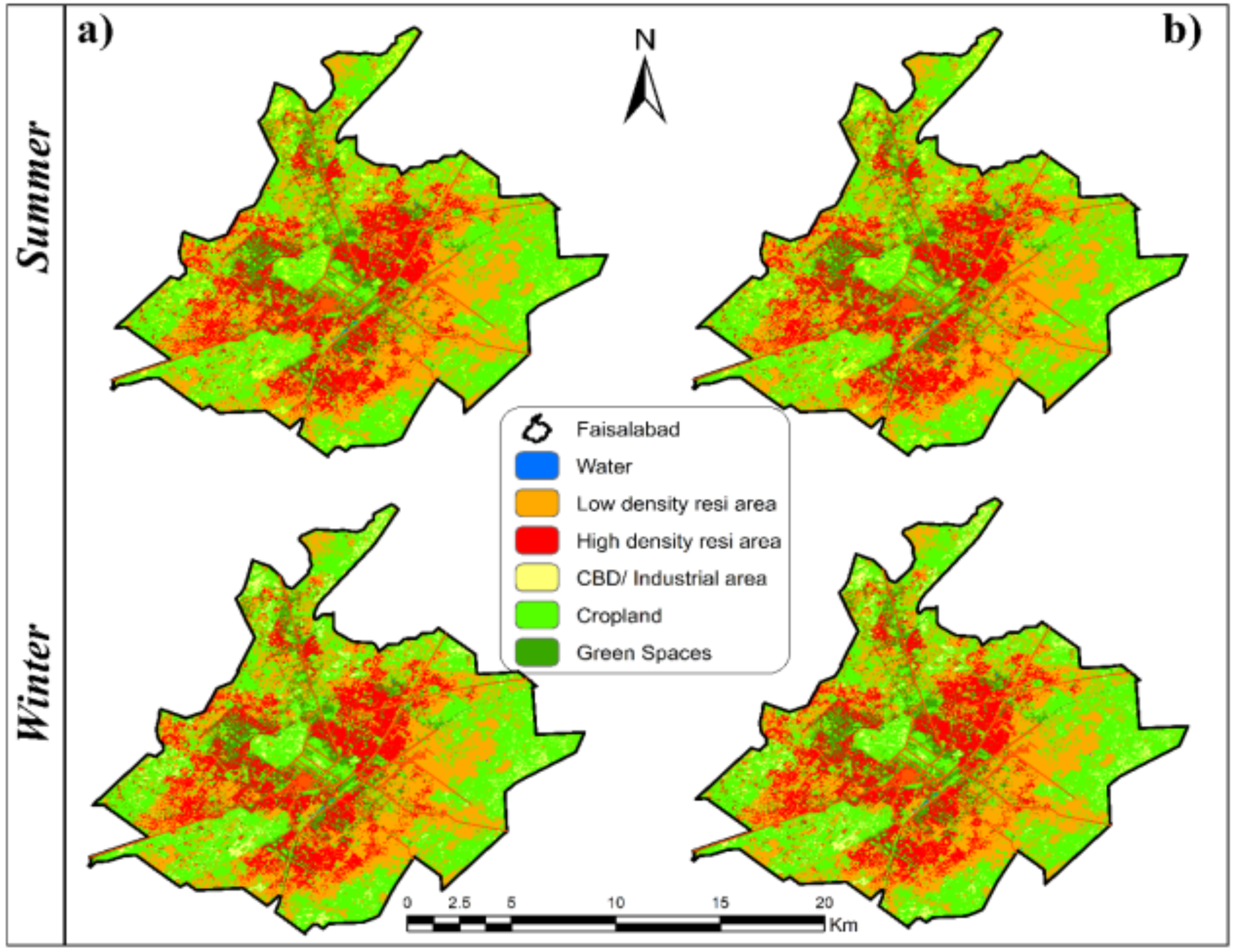
3]. Given the complexity of urban LULC spread, the SVM is a high accuracy classifier tested both in 1990 and 2018. The study of Reference [25] also shows that the SVM classifier can generate high-precision maps. The high accuracy of the map is related to the use of relevant digitized areas (rather than points) as ground data for classification, so its accuracy exceeds the standard 80% [26].
The derived maps of seasonal LULC showed that residential areas grew while vegetation and water cover declined in the same region between 1990 and 2018, which is compatible with previous studies [56]. The CA-Markov-Chain reliably predicts seasonal land use land cover types as showed by the strong consensus between the projected map of the year 2018 and the map prepared from the supervised rating. Based on variations in seasonal LULC between 1990 and 2018, the CA-Markov Chain predicted that unless other measures such as green spaces, cropland and water are implemented and identical trends exist, coverage of built-up area will tend to grow until 2048 at the cost of landcover. This conclusion is aligned with global projections that human growth would continue to grow at the cost of green space resulting in development of built-up areas [
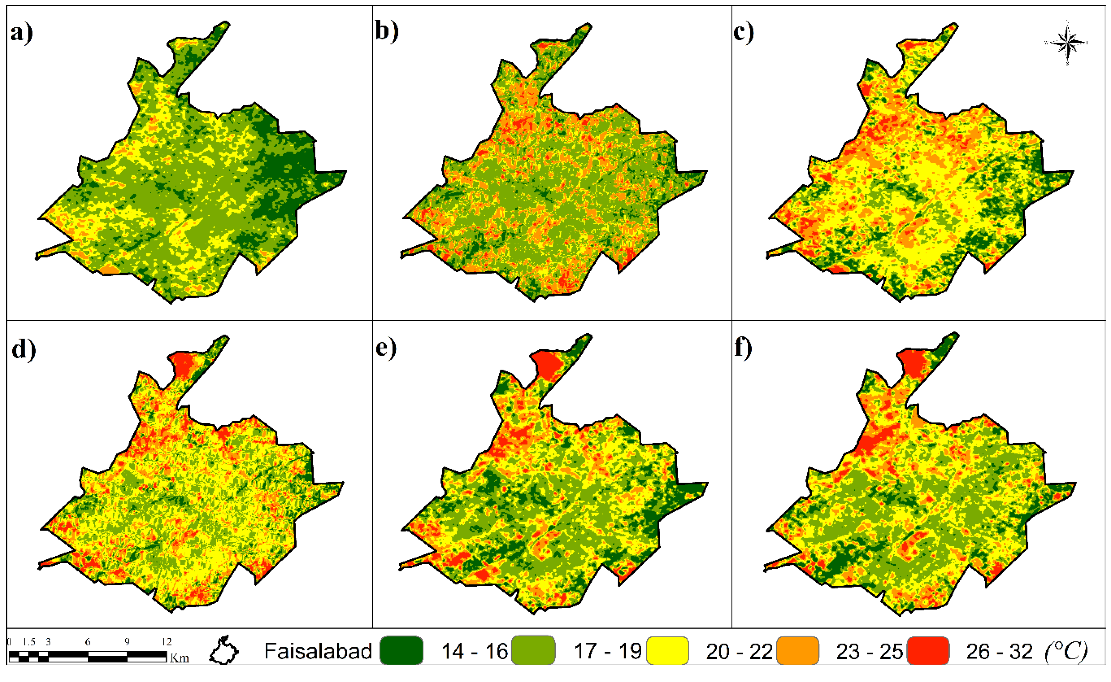
6,
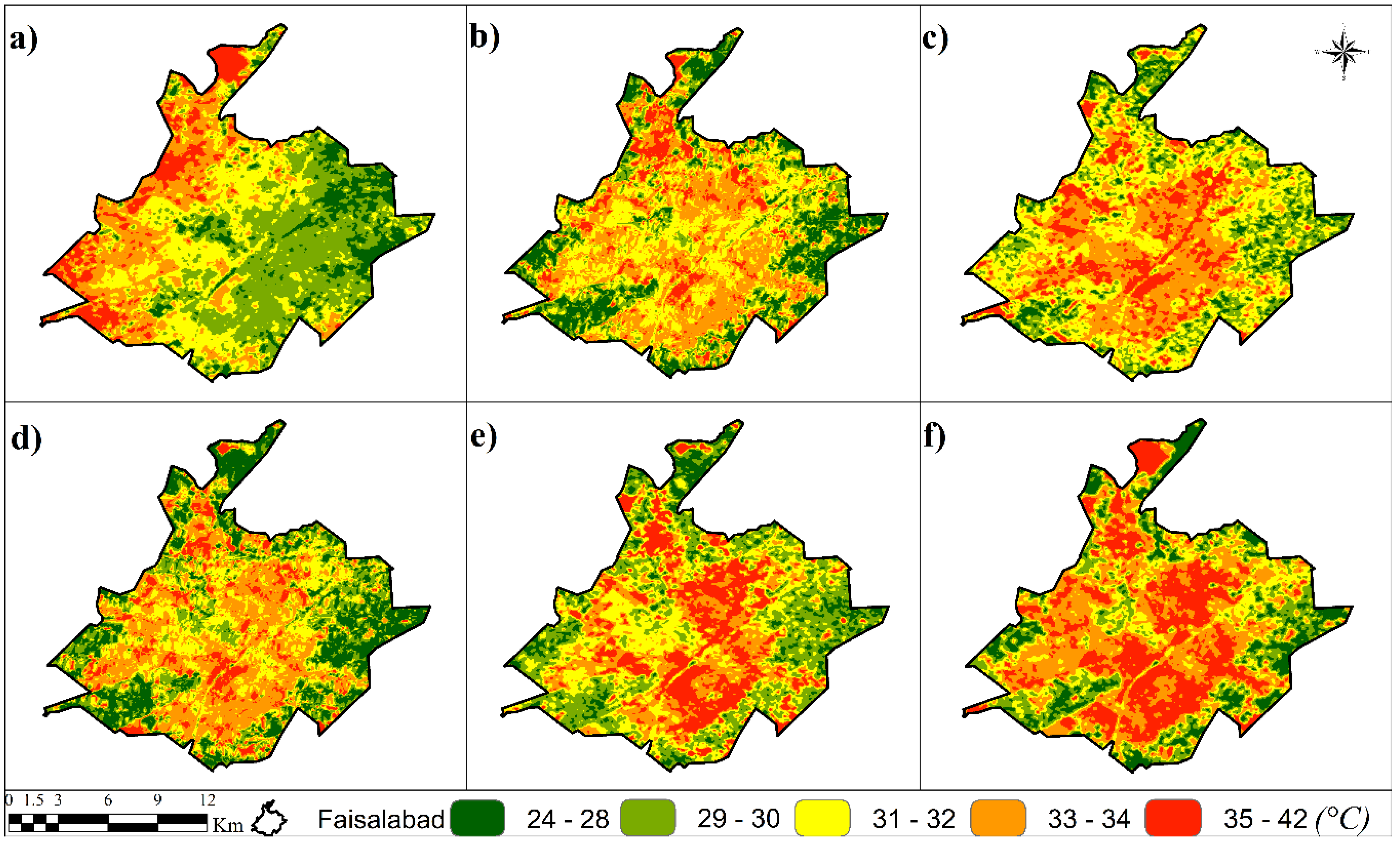
12]. The lowest temperature level region is predicted to decrease in this summer and winter study, whilst the region protected by warmer categories such as 36–42 °C and 26–32 °C is anticipated to increase. In addition to seasonal changes in LULC distribution, the increasing trends would see residential areas expand to the detriment of green spaces and water. The predicted temperature increases due to changes in urban development demonstrated by the land use land cover are also consistent with earlier research [4].

5. Conclusions

This study is aimed at exploring seasonal land cover indices and building the CA-Markov-Chain for predicting seasonal distribution of LST and LULC in Faisalabad. We found that the SVM algorithm applied to urban areas classified using Landsat 5, 7 and 8 imagery achieved an overall accuracy above 80%. The model achieved the function of closely matching the spatio-temporal distribution of seasonal types of LULC as defined by the SVM, driven by in situ observations. The average KIA predicted using CA-Markov between the summer and winter LULC and the distribution calculated using SVM classifier was 0.88 and 0.85. The proportion of summer season observed in Faisalabad between 1990 and 2018, LST in the categories 29–30 °C decreased by around 37% and 17–19 °C categories decreased by 22% in the winter season due to the rapid development of the CBD/industrial and residential area. During the same period, high LST coverage increased nearly 12% in the summer season (35–42 °C) and nearly 6% in the winter season (26–32°C), suggesting a strong biased trend of land heating in Faisalabad. The model is restricted because it only consider the effects of urban development on temperature changes and does not account for other factors. Although, the effective mitigation policies and revised urban expansion strategies have slightly shifted the patterns of LST. Overall, the findings of the present research demonstrate the value of medium-resolution satellite data, in forecasting potential land surface temperatures in urbanized areas. We conclude that unless control measures are taken, the acceleration of urbanization will increase warming and lead to higher temperatures in the future. The results of this study are essential to warn urban planners in order to understand the consequences of expansion on potential temperature changes and thermal comfort of urban residents. Future studies are, however, required to investigate the viability of these approaches and techniques at global and national spatial scales. The CA model was used for the identification of spatial distribution changes and Markov Chain analysis were used for the prediction of temporal resolution. In future researcher and policy makers will use this model to make new policies to control and manage the urban growth.

Author Contributions

A.T.: Conceptualization, Writing—review & editing, Methodology, Software, Formal analysis, Visualization, Data curation, Writing—original draft, Investigation. H.S.: Supervision, Visualization, Validation, Supervision, Investigation, Funding acquisition, Writing—review & editing. All authors have read and agreed to the published version of the manuscript.

Funding

This work is supported jointly by the National Key Research Development Program of China (No. 2017YFB0503604 and No. 2016YFB0502204), National Natural Science Foundation of China (No. 61971316) and State Key Laboratory of Satellite Navigation System and Equipment Technology.

Acknowledgments

We would like to pay special and heart whelming thanks to NASA-Earth data for providing us Landsat data and Clark Labs for providing us IDRISI Selva v_17.0 for analysis. We also admire Dr. Muhammad Imran from Institute of Geo-Information and Earth Observation (IGEO), PMAS-Arid Agriculture University, Rawalpindi for their facilitation at various stages of the field data collection.

Conflicts of Interest

The authors declare no conflict of interest.

References

  1. Hou, H.; Wang, R.; Murayama, Y. Scenario-based modelling for urban sustainability focusing on changes in cropland under rapid urbanization: A case study of Hangzhou from 1990 to 2035. Sci. Total Environ. 2019, 661, 422–431. [Google Scholar] [CrossRef] [PubMed]
  2. Hart, S.; Milstein, M. Global Sustainability and the Creative Destruction of Industries. Sloan Manag. Rev. 1999, 41, 23–33. [Google Scholar]
  3. Cohen, B. Urban growth in developing countries: A review of current trends and a caution regarding existing forecasts. World Dev. 2004, 32, 23–51. [Google Scholar] [CrossRef]
  4. Day, K.; Alfonzo, M.; Chen, Y.; Guo, Z.; Lee, K.K. Overweight, Obesity, And inactivity and urban design in rapidly growing Chinese cities. Health Place 2013, 21, 29–38. [Google Scholar] [CrossRef] [PubMed]
  5. Hu, Y.; Jia, G. Influence of land use change on urban heat island derivedfrom multi-sensor data. Int. J. Climatol. 2010, 30, 1382–1395. [Google Scholar] [CrossRef]
  6. Araya, Y.H.; Cabral, P. Analysis and modeling of urban land cover change in Setúbal and Sesimbra, Portugal. Remote Sens. 2010, 2, 1549–1563. [Google Scholar] [CrossRef] [Green Version]
  7. Mushore, T.D.; Mutanga, O.; Odindi, J.; Dube, T. Assessing the potential of integrated Landsat 8 thermal bands, with the traditional reflective bands and derived vegetation indices in classifying urban landscapes. Geocarto Int. 2017, 32, 886–899. [Google Scholar] [CrossRef]
  8. Chen, X.L.; Zhao, H.M.; Li, P.X.; Yin, Z.Y. Remote sensing image-based analysis of the relationship between urban heat island and land use/cover changes. Remote Sens. Environ. 2006, 104, 133–146. [Google Scholar] [CrossRef]
  9. Hashem, N.; Balakrishnan, P. Change analysis of land use/land cover and modelling urban growth in Greater Doha, Qatar. Ann. GIS 2015, 21, 233–247. [Google Scholar] [CrossRef]
  10. Ahmed, B.; Kamruzzaman, M.D.; Zhu, X.; Shahinoor Rahman, M.D.; Choi, K. Simulating land cover changes and their impacts on land surface temperature in dhaka, bangladesh. Remote Sens. 2013, 5, 5969–5998. [Google Scholar] [CrossRef] [Green Version]
  11. Hasanlou, M.; Mostofi, N. Investigating Urban Heat Island Effects and Relation Between Various Land Cover Indices in Tehran City Using Landsat 8 Imagery. In Proceedings of the 1st International Electronic Conference on Remote Sensing, Basel, Switzerland, 5–22 July 2015; pp. 1–11. [Google Scholar]
  12. Ahmed, B.; Ahmed, R. Modeling urban land cover growth dynamics using multioral satellite images: A case study of Dhaka, Bangladesh. ISPRS Int. J. Geo-Inf. 2012, 1, 3–31. [Google Scholar] [CrossRef] [Green Version]
  13. Wilson, M. Climate Change. Can. Vet. J. La Rev. Vet. Can. 2020, 61, 225. [Google Scholar]
  14. Saitoh, T.S.; Shimada, T.; Hoshi, H. Modeling and simulation of the Tokyo urban heat island. Atmos. Environ. 1996, 30, 3431–3442. [Google Scholar] [CrossRef]
  15. Hoffmann, P.; Krueger, O.; Schlünzen, K.H. A statistical model for the urban heat island and its application to a climate change scenario. Int. J. Climatol. 2012, 32, 1238–1248. [Google Scholar] [CrossRef]
  16. Charles, N.; Reneth, M.; Shakespear, M.; Virginia, M. Climate change adaptation for rural communities dependent on agriculture and tourism in marginal farming areas of the Hwange District, Zimbabwe. African J. Agric. Res. 2014, 9, 2045–2054. [Google Scholar] [CrossRef] [Green Version]
  17. Manatsa, D.; Mushore, T.; Lenouo, A. Improved predictability of droughts over southern Africa using the standardized precipitation evapotranspiration index and ENSO. Theor. Appl. Climatol. 2017, 127, 259–274. [Google Scholar] [CrossRef]
  18. Mazvimavi, D. Investigating changes over time of annual rainfall in Zimbabwe. Hydrol. Earth Syst. Sci. 2010, 14, 2671–2679. [Google Scholar] [CrossRef] [Green Version]
  19. Zhang, Q.; Wang, J.; Peng, X.; Gong, P.; Shi, P. Urban built-up land change detection with road density and spectral information from multi-temporal Landsat TM data. Int. J. Remote Sens. 2002, 23, 3057–3078. [Google Scholar] [CrossRef]
  20. Bhalli, M.N.; Ghaffar, A.; Shirazi, S.A.; Parveen, N. Use of Multi-Temporal Digital Data To Monitor Lulc Changes in Faisalabad-Pakistan. Pak. J. Sci. 2013, 65, 58–62. [Google Scholar]
  21. Nasar-u-minAllah Bhalli, M.; Ghaffar, A.; Shirazi, S.A.; Parveen, N.; Anwar, M.M. Change detection analysis of land use by using geospatial techniques: A case study of faisalabad- pakistan. Sci. Int. (Lahore) 2012, 24, 539–546. [Google Scholar]
  22. Bernstein, L.S.; Adler-Golden, S.M.; Sundberg, R.L.; Levine, R.Y.; Perkins, T.C.; Berk, A.; Ratkowski, A.J.; Felde, G.; Hoke, M.L. Validation of the QUick atmospheric correction (QUAC) algorithm for VNIR-SWIR multi- and hyperspectral imagery. Proc. SPIE 2005, 5806, 668. [Google Scholar] [CrossRef]
  23. Tariq, A.; Riaz, I.; Ahmad, Z.; Amin, M.; Kausar, R.; Andleeb, S.; Farooqi, M.A.; Rafiq, M. Land surface temperature relation with normalized satellite indices for the estimation of spatio-temporal trends in temperature among various land use land cover classes of an arid Potohar region using Landsat data. Environ. Earth Sci. 2020, 79, 1–15. [Google Scholar] [CrossRef]
  24. Mushore, T.D.; Odindi, J.; Dube, T.; Mutanga, O. Prediction of future urban surface temperatures using medium resolution satellite data in Harare metropolitan city, Zimbabwe. Build. Environ. 2017, 122, 397–410. [Google Scholar] [CrossRef]
  25. Adelabu, S.; Mutanga, O.; Adam, E.; Cho, M.A. Exploiting machine learning algorithms for tree species classification in a semiarid woodland using RapidEye image. J. Appl. Remote Sens. 2013, 7, 073480. [Google Scholar] [CrossRef]
  26. Omran, E.-S.E. Detection of Land-Use and Surface Temperature Change at Different Resolutions. J. Geogr. Inf. Syst. 2012, 04, 189–203. [Google Scholar] [CrossRef] [Green Version]
  27. Jensen, J.R. Urban/suburban land use analysis. In Manual of Remote Sensing, 2nd ed.; Colwell, R.N., Ed.; American Society of Photogrammetry: Falls Church, VA, USA, 1983; Volume 2, pp. 1571–1666. [Google Scholar]
  28. Tucker, C.J. Red and photographic infrared linear combinations for monitoring vegetation. Remote Sens. Environ. 1979, 8, 127–150. [Google Scholar] [CrossRef] [Green Version]
  29. Mann, H.B.; Whitney, D.R. On a Test of Whether one of Two Random Variables is Stochastically Larger than the Other. Ann. Math. Stat. 1947, 18, 50–60. [Google Scholar] [CrossRef]
  30. Zhao, H.; Chen, X. Use of normalized difference bareness index in quickly mapping bare areas from TM/ETM+. Int. Geosci. Remote Sens. Symp. 2005, 3, 1666–1668. [Google Scholar]
  31. McFeeters, S.K. The use of the Normalized Difference Water Index (NDWI) in the delineation of open water features. Int. J. Remote Sens. 1996, 17, 1425–1432. [Google Scholar] [CrossRef]
  32. Xu, H. Modification of normalised difference water index (NDWI) to enhance open water features in remotely sensed imagery. Int. J. Remote Sens. 2006, 27, 3025–3033. [Google Scholar] [CrossRef]
  33. Kawamura, M.; Jayamana, S.; Tsujiko, Y. Relation between social and environmental conditions in Colombo Sri Lanka and the Urban Index estimated by satellite remote sensing data. Intern. Arch. Photogramm. Remote Sens. 1996, 31, 321–326. [Google Scholar]
  34. Zha, Y.; Gao, J.; Ni, S. Use of normalized difference built-up index in automatically mapping urban areas from TM imagery. Int. J. Remote Sens. 2003, 24, 583–594. [Google Scholar] [CrossRef]
  35. Huete, A.R. A soil-adjusted vegetation index (SAVI). Remote Sens. Environ. 1988, 25, 295–309. [Google Scholar] [CrossRef]
  36. Gutman, G.; Ignatov, A. The derivation of the green vegetation fraction from NOAA/AVHRR data for use in numerical weather prediction models. Int. J. Remote Sens. 1998, 19, 1533–1543. [Google Scholar] [CrossRef]
  37. Liu, H.Q.; Huete, A. Feedback based modification of the NDVI to minimize canopy background and atmospheric noise. IEEE Trans. Geosci. Remote Sens. 1995, 33, 457–465. [Google Scholar] [CrossRef]
  38. Datta, D.; Prasad, M.; Mandla, V.R. Study of various factors influence on land surface temperature in urban environment. J. Urban Environ. Eng. 2017, 11, 58–62. [Google Scholar] [CrossRef]
  39. Avdan, U.; Jovanovska, G. Algorithm for automated mapping of land surface temperature using LANDSAT 8 satellite data. J. Sensors 2016, 2016, 1–8. [Google Scholar] [CrossRef] [Green Version]
  40. Artis, D.A.; Carnahan, W.H. Survey of emissivity variability in thermography of urban areas. Remote Sens. Environ. 1982, 12, 313–329. [Google Scholar] [CrossRef]
  41. Stathopoulou, M.; Cartalis, C.; Chrysoulakis, N. Using midday surface temperature to estimate cooling degree-days from NOAA-AVHRR thermal infrared data: An application for Athens, Greece. Sol. Energy 2006, 80, 414–422. [Google Scholar] [CrossRef]
  42. Weng, Q.; Liu, H.; Lu, D. Assessing the effects of land use and land cover patterns on thermal conditions using landscape metrics in city of Indianapolis, United States. Urban Ecosyst. 2007, 10, 203–219. [Google Scholar] [CrossRef]
  43. Yang, F. Turbo decoder using local subsidiary maximum likelihood decoding in prior estimation of the extrinsic information. J. Electron. 2004, 21, 89–96. [Google Scholar] [CrossRef]
  44. Mushore, T.D.; Mutanga, O.; Odindi, J.; Dube, T. Determining extreme heat vulnerability of Harare Metropolitan City using multispectral remote sensing and socio-economic data. J. Spat. Sci. 2018, 63, 173–191. [Google Scholar] [CrossRef]
  45. Triantakonstantis, D.; Mountrakis, G. Urban Growth Prediction: A Review of Computational Models and Human Perceptions. J. Geogr. Inf. Syst. 2012, 04, 555–587. [Google Scholar] [CrossRef] [Green Version]
  46. Keshtkar, H.; Voigt, W. A spatiotemporal analysis of landscape change using an integrated Markov chain and cellular automata models. Model. Earth Syst. Environ. 2016, 2, 1–13. [Google Scholar] [CrossRef] [Green Version]
  47. SHAPIRO, S.S.; WILK, M.B. An analysis of variance test for normality (complete samples)†. Biometrika 1965, 52, 591–611. [Google Scholar] [CrossRef]
  48. Aaviksoo, K. Simulating vegetation dynamics and land use in a mire landscape using a Markov model. Landsc. Urban Plan. 1995, 31, 129–142. [Google Scholar] [CrossRef]
  49. García-Frapolli, E.; Ayala-Orozco, B.; Bonilla-Moheno, M.; Espadas-Manrique, C.; Ramos-Fernández, G. Biodiversity conservation, traditional agriculture and ecotourism: Land cover/land use change projections for a natural protected area in the northeastern Yucatan Peninsula, Mexico. Landsc. Urban Plan. 2007, 83, 137–153. [Google Scholar] [CrossRef]
  50. Mosammam, H.M.; Nia, J.T.; Khani, H.; Teymouri, A.; Kazemi, M. Monitoring land use change and measuring urban sprawl based on its spatial forms: The case of Qom city. Egypt. J. Remote Sens. Sp. Sci. 2017, 20, 103–116. [Google Scholar]
  51. Arsanjani, J.J.; Helbich, M.; Kainz, W.; Boloorani, A.D. Integration of logistic regression, Markov chain and cellular automata models to simulate urban expansion. Int. J. Appl. Earth Obs. Geoinf. 2012, 21, 265–275. [Google Scholar] [CrossRef]
  52. Sayemuzzaman, M.; Jha, M.K. Modeling of Future Land Cover Land Use Change in North Carolina Using Markov Chain and Cellular Automata Model. Am. J. Eng. Appl. Sci. 2014, 7, 295–306. [Google Scholar] [CrossRef]
  53. Birnbaum, Z.W. On a use of the Mann-Whitney statistic. In Proceedings of the Third Berkeley Symposium on Mathematical Statistics and Probability, Volume 1: Contributions to the Theory of Statistics; The Regents of the University of California: Oakland, CA, USA, 1956. [Google Scholar]
  54. Pauleit, S.; Ennos, R.; Golding, Y. Modeling the environmental impacts of urban land use and land cover change—A study in Merseyside, UK. Landsc. Urban Plan. 2005, 71, 295–310. [Google Scholar] [CrossRef]
  55. Masek, J.G.; Lindsay, F.E.; Goward, S.N. Dynamics of urban growth in the Washington DC metropolitan area, 1973-1996, from Landsat observations. Int. J. Remote Sens. 2000, 21, 3473–3486. [Google Scholar] [CrossRef]
  56. Kamusoko, C.; Gamba, J.; Murakami, H. Monitoring Urban Spatial Growth in Harare Metropolitan Province, Zimbabwe. Adv. Remote Sens. 2013, 2, 322–331. [Google Scholar] [CrossRef] [Green Version]
Figure 1. Geographical location of study area and points were used for statistically exploring the relationship between vegetation indices and temperature.
Remotesensing 12 03402 g001
Figure 2. Flow chart of the general methodology.
Remotesensing 12 03402 g002
Figure 3. Changes mapping of surface temperature during the summer seasons were observed in (a) 1990, (b) 1998, (c) 2004, (d) 2008, (e) 2013 and (f) 2018.
Remotesensing 12 03402 g003
Figure 4. Changes in mapping of surface temperature during the winter seasons were observed in (a) 1990, (b) 1998, (c) 2004, (d) 2008, (e) 2013 and (f) 2018.
Remotesensing 12 03402 g004
Figure 5. Prediction of seasonal LST from Urban Index by using Linear model.
Remotesensing 12 03402 g005
Figure 6. Comparison of seasonal surface temperature derived from thermal band with UI.
Remotesensing 12 03402 g006
Figure 7. 2018 summer and winter LULC mapping with (a) supervised classification and (b) CA-Markov-Chain prediction.
Remotesensing 12 03402 g007
Figure 8. Predicted seasonal distribution of LULC in (a) 2028, (b) 2038 and (c) 2048.
Remotesensing 12 03402 g008
Table 1. Landsat data collected during the summer and winter.
YearsSensorPathRowSummer DateAir Temperature (°C)Relative Humidity (%)Winter DateAir Temperature (°C)Relative Humidity (%)Processing Level
1990TM1493822 May 199034.461.011 November 1990 31.058.0TIER 1
1998TM1493810 May 199833.359.017 November 199830.063.0TIER 1
2004ETM1493830 May 200434.751.009 November 200430.561.0TIER 1
2008ETM1493816 May 200835.355.004 November 200831.062.0TIER 1
2013OLI/TIRS1493827 May 201335.254.010 November 201331.556.0TIER 1
2018OLI/TIRS1493802 June 201835.448.408 November 201831.753.0TIER 1
Table 2. Land Use and Land Cover (LULC) classes from the field survey in Faisalabad city.
LULC ClassAbbreviationsDescription
Central Business District/Industrial areaCBD/I. AreaAreas with very high density of buildings and a very high proportion of impervious surface that include central business district and industrial areas.
High density residentialHDR High density residential areas and areas under residential development (bare or impervious) with low vegetation fraction.
Low density residentialLDR Established low and medium density residential areas with high vegetation fraction.
CroplandsCropsAreas where intra-urban agriculture is practiced including research sites could be bare in the summer and winter seasons.
Green-spacesG. SpacesAreas covered by grasslands, shrubs and clusters of trees characterized by high vegetation fraction even during the summer and winter season.
Water/WetlandWaterAreas covered by water bodies or wetlands.
Table 3. Indices of predicting Land-Surface-Temperature (LST) for 2028, 2038 and 2048.
IndexNameFormulation (Landsat 5/Landsat 7)Formulation (Landsat 8)References
NDVINormalized Difference Vegetation Index ( B a n d 4 B a n d 3 ) ( B a n d 4 + B a n d 3 )
( NIR     Red ) ( NIR   +   Red )
( B a n d 5 B a n d 4 ) ( B a n d 5 + B a n d 4 )
( N I R R e d ) ( N I R + R e d )
[28]
BIBare Soil Index ( B a n d 5 + B a n d 3 ) ( B a n d 4 + B a n d 1 ) ( B a n d 5 + B a n d 3 ) + ( B a n d 4 + B a n d 1 )
( S W I R 1 + R E D ) ( N I R + B l u e ) ( S W I R 1 + R E D ) + ( N I R + B l u e )
( B a n d 6 + B a n d 4 ) ( B a n d 5 + B a n d 2 ) ( B a n d 6 + B a n d 4 ) + ( B a n d 5 + B a n d 2 )
( S W I R 1 + R E D ) ( N I R + B l u e ) ( S W I R 1 + R E D ) + ( N I R + B l u e )
[29]
NDBaINormalized Difference Bareness Index ( B a n d 5 B a n d 6 ) ( B a n d 5 + B a n d 6 )
( SWIR 1 TIRS 1 ) ( SWIR 1 + TIRS 1 )
( B a n d 6 B a n d 10 ) ( B a n d 6 + B a n d 10 )
( S W I R 1 T I R S 1 ) ( S W I R 1 + T I R S 1 )
[30]
NDWINormalized Difference Water Index ( B a n d 3 B a n d 5 ) ( B a n d 3 + B a n d 5 )
( Red   SWIR 1 ) ( Red   + SWIR 1 )
( B a n d 4 B a n d 6 ) ( B a n d 4 + B a n d 6 )
( R e d S W I R 1 ) ( R e d + S W I R 1 )
[31]
MNDWIModified Normalized Difference Water Index ( Band 2 Band 4 ) ( Band 2 + Band 4 )
( Green NIR ) ( Green + NIR )
( B a n d 3 B a n d 5 ) ( B a n d 3 + B a n d 5 )
( G r e e n N I R ) ( G r e e n + N I R )
[32]
UIUrban Index ( B a n d 7 B a n d 4 ) ( B a n d 7 + B a n d 4 )
( S W I R 2 N I R ) ( S W I R 2 + N I R )
( B a n d 7 B a n d 5 ) ( B a n d 7 + B a n d 5 )
( S W I R 2 N I R ) ( S W I R 2 + N I R )
[33]
NDBINormalized Difference Built up Area Index ( B a n d 5 B a n d 4 ) ( B a n d 5 + B a n d 4 )
( S W I R 1 N I R ) ( S W I R 1 + N I R )
( B a n d 6 B a n d 5 ) ( B a n d 6 + B a n d 5 )
( S W I R 1 N I R ) ( S W I R 1 + N I R )
[34]
SAVISoil Adjusted Vegetation Index ( Band 4 Band 3 ) ( Band 4 + Band 3 + L ) × ( L + 1 )
( N I R R E D ) N I R + R E D + L × ( L + 1 )
( Band 5 Band 4 ) ( Band 5 + Band 4 + L ) × ( L + 1 )
( N I R R E D ) N I R + R E D + L × ( L + 1 )
[35]
FVGVegetation fraction ( N D V I N D V I S o i l ) ( N D V I V e g + N D V I S o i l ) ( N D V I N D V I S o i l ) ( N D V I V e g + N D V I S o i l ) [36]
EVIEnhanced Vegetation Index ( Band 4 Band 3 ) Band 4 + 6 × Band 3 7.5 × Band 1 + 1
( NIR RED ) NIR + 6 × RED 7.5 × BLUE + 1
( Band 5 Rand 4 ) Band 5 + 6 × Band 4 7.5 × Band 2 + 1
( NIR RED ) NIR + 6 × RED 7.5 × BLUE + 1
[37]
Table 4. Landsat 5, 7 and 8 Thermal band calibration constants & rescaling.
Sensor K 1 [ W ( m 2   sr   µ m ) ] K 2 [ W ( m 2   sr   µ m )   ] Rescaling
TM607.761260.56
ETM666.091282.71
OLI/TIRS774.88531321.0789ML 0.0003342
AL 0.10
Table 5. The proportion of seasonal LULC changes from 1990 to 2018.
LULC TypeSummer Area in km2 and (Percentage)Winter Area in km2 and (Percentage)
199019982004200820132018199019982004200820132018
CBD/I Area1.53 (0.76)3.05 (1.51)4.67 (2.31)5.18 (2.56)6.05 (3.00)6.35 (3.14)1.53 (0.76)3.05 (1.51)4.67 (2.31)5.18 (2.56)6.05 (3.00)6.35 (3.14)
HDR8.77 (4.35)11.34 (5.62)11.93 (5.91)13.05 (6.07)17.74 (9.29)22.23 (11.02)8.77 (4.35)11.34 (5.62)11.93 (5.91)13.05 (6.07)17.74 (9.29)22.23 (11.02)
LDR57.53 (28.51)73.10 (36.23)78.64 (38.98)82.12 (40.70)95.39 (47.28)108.34 (53.70)57.53 (28.51)73.10 (36.23)78.64 (38.98)82.12 (40.70)95.39 (47.28)108.34 (53.70)
G. Spaces18.70 (9.27)19.31 (9.57)36.37 (18.02)31.34 (15.53)18.40 (9.12)16.40 (8.13)13.25 (6.57)17.57 (8.71)23.68 (11.73)19.85 (9.84)9.40 (4.66)6.74 (3.34)
Crops114.31 (56.65)89.73 (44.47)70.02 (34.71)68.73 (34.06)63.07 (31.26)47.92 (23.75)114.49 (56.74)88.94 (44.08)69.46 (34.43)67.80 (33.61)60.92 (30.19)45.77 (22.68)
Water0.93 (0.46)5.23 (2.59)0.14 (0.07)1.35 (0.67)0.11 (0.05)0.52 (0.26)1.38 (0.68)1.11 (0.55)1.01 (0.50)1.29 (0.64))1.47 (0.73)0.84 (0.41)
Table 6. Average LST (summer and winter) responses to urban growth in Faisalabad City.
LSTSummer Area in km2 and (Percentage) LSTWinter Area in km2 and (Percentage)
Summer199019982004200820132018Winter199019982004200820132018
24–2811.06 (5.56)29.62 (14.88)12.93 (6.49)28.77 (14.45)16.11 (8.09)21.40 (10.75)14–1632.20 (16.13)12.73 (6.38)33.88 (16.98)31.89 (15.98)27.04 (13.55)17.59 (8.81)
29–30107.95 (54.23)30.49 (15.32)35.59 (17.88)36.58 (18.37)53.07 (26.66)34.38 (17.24)17–19118.16 (59.21)108.53 (54.38)54.17 (27.14)59.73 (29.93)73.03 (36.59)75.23 (37.69)
31–3261.65 (30.97)60.13 (30.20)67.55 (33.93)46.52 (23.37)53.08 (26.67)45.75 (22.98)20–2242.05 (21.07)40.75 (20.42)70.83 (35.49)57.57 (28.85)56.46 (28.29)62.76 (31.45)
33–3412.96 (6.51)62.20 (31.24)58.35 (29.31)61.08 (30.68)40.26 (20.22)74.57 (37.46)23–2507.52 (3.77)29.95 (15.01)32.23 (16.15)42.54 (21.32)30.09 (15.08)30.43 (15.25)
35–420.65 (0.33)16.64 (8.36)12.73 (6.39)17.43 (8.75)23.03 (11.57)25.27 (12.69)26–3201.01 (0.50)7.61 (3.81)8.85 (4.43)8.51 (4.27)13.38 (6.71)13.47 (6.75)
Table 7. Correlation of temperature (Summer) with indices of urban as well as vegetation.
LSTNDVIBINDBaINDWIMNDWIUINDBISAVIEVIFVG
LST1.0000−0.71330.74610.04550.61200.72300.89620.8801−0.7191−0.0257−0.7133
NDVI−0.71331.0000−0.8148−0.0322−0.7956−0.9040−0.8918−0.85560.91380.12021.0000
BI0.7461−0.81481.00000.43900.58700.81510.95410.9828−0.9018−0.1310−0.8148
NDBaI0.0455−0.03220.43901.0000−0.3435−0.10590.23210.3089−0.0483−0.0809−0.0322
NDWI0.6120−0.79560.5870−0.34351.00000.90980.74130.6455−0.8674−0.0339−0.7956
MNDWI0.7230−0.90400.8151−0.10590.90981.00000.93160.8822−0.9820−0.1045−0.9040
UI0.8962−0.89180.95410.23210.74130.93161.00000.9788−0.9698−0.1276−0.8918
NDBI0.8801−0.85560.98280.30890.64550.88220.97881.0000−0.9398−0.1424−0.8556
SAVI−0.71910.9138−0.9018−0.0483−0.8674−0.9820−0.9698−0.93981.00000.10840.9138
EVI−0.02570.1202−0.1310−0.0809−0.0339−0.1045−0.1276−0.14240.10841.00000.1202
FVG−0.71331.0000−0.8148−0.0322−0.7956−0.9040−0.8918−0.85560.91380.12021.0000
Table 8. Correlation of temperature (winter) with indices of urban as well as vegetation.
LSTNDVIBINDBaINDWIMNDWIUINDBISAVIEVIFVG
LST1.0000−0.53530.84620.2641−0.17000.12370.92120.9907−0.6353−0.0692−0.2353
NDVI−0.53531.00000.32370.2865−0.7157−0.9757−0.8786−0.76981.0000−0.37891.0000
BI0.84620.32371.00000.9706−0.7899−0.50930.11550.26030.3237−0.45210.3237
NDBaI0.26410.28650.97061.0000−0.8226−0.47410.17570.34340.2865−0.40090.2865
NDWI−0.1700−0.7157−0.7899−0.82261.00000.82750.30730.1052−0.71570.4324−0.7157
MNDWI0.1237−0.9757−0.5093−0.47410.82751.00000.76510.6329−0.97570.4364−0.9757
UI0.9212−0.87860.11550.17570.30730.76511.00000.9699−0.87860.2160−0.8786
NDBI0.9907−0.76980.26030.34340.10520.63290.96991.0000−0.76980.1447−0.7698
SAVI−0.63531.00000.32370.2865−0.7157−0.9757−0.8786−0.76981.0000−0.37891.0000
EVI−0.0692−0.3789−0.4521−0.40090.43240.43640.21600.1447−0.37891.0000−0.3789
FVG−0.23531.00000.32370.2865−0.7157−0.9757−0.8786−0.76981.0000−0.37891.0000
Table 9. Statistical analysis of coordination between supervised classification and CA-Markov Chain based on the 2018 prediction.
LULC TypeKappa Index of Agreement (KIA)
SummerWinter
CBD/Industrial0.830.85
High density residential area0.850.86
Low density residential area0.840.86
Green-spaces0.890.84
Croplands0.810.79
Water/Wetland0.780.80
Table 10. Change in proportion of summer and winter LULC types between 2028 and 2048.
LULC TypeSummer Area in km2 and (Percentage)Winter Area in km2 and (Percentage)
202820382048202820382048
CBD/I. Area6.89 (3.41)7.40 (3.67)7.92 (3.93)6.89 (3.41)7.40 (3.67)7.92 (3.93)
HDR22.92 (11.36)23.43 (11.61)24.52 (12.15)22.92 (11.36)23.43 (11.61)24.52 (12.15)
LDR113.92 (56.46)118.49 (58.72)122.61 (60.77)113.92 (56.46)118.49 (58.72)122.61 (60.77)
G. Spaces15.86 (7.86)14.56 (7.22)12.82 (6.35)12.80 (6.34)11.77 (5.84)9.04 (4.48)
Crops41.60 (20.62)37.13 (18.40)33.51 (16.61)44.30 (21.96)39.83 (19.74)37.11(18.39)
Water0.58 (0.29)0.77 (0.38)0.39 (0.19)0.94 (0.47)0.95 (0.47)0.57 (0.28)
Table 11. Predicted changes in seasonal surface temperature due to urban growth.
LSTSummer Area in km2 and (Percentage)LSTWinter Area in km2 and (Percentage)
202820382048202820382048
24–2813.52 (6.71)9.92 (4.93)6.32 (3.14)14–1613.99 (7.01)10.39 (5.30)6.79 (3.47)
29–3028.98 (14.39)25.38 (12.60)21.78 (10.82)17–1971.63 (35.91)64.43 (32.89)60.83 (31.05)
31–3240.97 (20.34)37.37 (18.56)33.77 (16.77)20–2259.16 (29.66)55.56 (28.36)51.96 (26.53)
33–3480.04 (39.75)85.44 (42.43)90.84 (45.11)23–2535.83 (17.96)41.23 (21.05)46.63 (23.80)
35–4237.87 (18.80)43.27 (21.49)48.67 (24.17)26–3218.87 (9.46)24.27 (12.39)29.67 (15.15)
Publisher’s Note: MDPI stays neutral with regard to jurisdictional claims in published maps and institutional affiliations.

