Discriminating Forest Successional Stages, Forest Degradation, and Land Use in Central Amazon Using ALOS/PALSAR-2 Full-Polarimetric Data

Abstract

We discriminated different successional forest stages, forest degradation, and land use classes in the Tapajós National Forest (TNF), located in the Central Brazilian Amazon. We used full polarimetric images from ALOS/PALSAR-2 that have not yet been tested for land use and land cover (LULC) classification, neither for forest degradation classification in the TNF. Our specific objectives were: (1) to test the potential of ALOS/PALSAR-2 full polarimetric images to discriminate LULC classes and forest degradation; (2) to determine the optimum subset of attributes to be used in LULC classification and forest degradation studies; and (3) to evaluate the performance of Random Forest (RF) and Support Vector Machine (SVM) supervised classifications to discriminate LULC classes and forest degradation. PALSAR-2 images from 2015 and 2016 were processed to generate Radar Vegetation Index, Canopy Structure Index, Volume Scattering Index, Biomass Index, and Cloude–Pottier, van Zyl, Freeman–Durden, and Yamaguchi polarimetric decompositions. To determine the optimum subset, we used principal component analysis in order to select the best attributes to discriminate the LULC classes and forest degradation, which were classified by RF. Based on the variable importance score, we selected the four first attributes for 2015, alpha, anisotropy, volumetric scattering, and double-bounce, and for 2016, entropy, anisotropy, surface scattering, and biomass index, subsequently classified by SVM. Individual backscattering indexes and polarimetric decompositions were also considered in both RF and SVM classifiers. Yamaguchi decomposition performed by RF presented the best results, with an overall accuracy (OA) of 76.9% and 83.3%, and Kappa index of 0.70 and 0.80 for 2015 and 2016, respectively. The optimum subset classified by RF showed an OA of 75.4% and 79.9%, and Kappa index of 0.68 and 0.76 for 2015 and 2016, respectively. RF exhibited superior performance in relation to SVM in both years. Polarimetric attributes exhibited an adequate capability to discriminate forest degradation and classes of different ecological succession from the ones with less vegetation cover.

1. Introduction

The Legal Amazonia, also known as the Brazilian Amazon, covers a continuous area of more than five million square kilometers [1], with approximately three million and two hundred thousand square kilometers of tropical forest [2]. The Amazon forest plays an important role in the global carbon cycle [3] and biodiversity conservation [4] and provides diverse ecosystem services, many of which with considerable economic value [5]. However, Brazil is among the tropical countries with the highest rates of forest loss [6]. Between 2010 and 2019, the Legal Amazonia, which includes the states of Acre, Amapá, Amazonas, Mato Grosso, Pará, Rondônia, Roraima, Tocantins, and part of the Maranhão, lost about 65,348 km² of its forest [7]. This loss corresponds to the gross carbon emission of 4366 million metric tons of carbon dioxide (Mt CO₂) in this area [8]. The latest deforestation rate (from August 2018 to July 2019), released by the Project of Deforestation Monitoring of the Brazilian Amazon Forest by satellite (PRODES), showed a 29.5% deforestation increase in relation to the deforestation rate from 2018 [7].

The last decade’s forest loss is due mainly to the unsustainable expansion of agriculture, cattle ranching, urbanization, illegal logging, and mining [9,10]. Moreover, the number of active fires in 2019 was the highest since 2010 [11], when the Amazonia experienced a severe drought caused by El Niño and Atlantic Ocean warming events [12]. In 2019, a total of 89,186 heat points were identified in the Legal Amazonia, corresponding to an increase of 30.5% when compared to the same period in 2018 (68,345 heat points) [13]. Fires occurred mainly in Pará (27,412 km²), Amazonas (15,074 km²), Mato Grosso (14,638 km²), and Rondônia (11,611 km²) states, contributing significantly to the forest loss and degradation [14].

Intensive forest degradation and deforestation observed in the last decades has led to significant losses of water resources, forest function, growing carbon balance variations, increase habitat fragmentations [15,16], and biodiversity threats [17,18]. In 2019, the Brazilian environmental protection policies were weakened because of the fewer economic resources destined for environmental monitoring by the two federal environmental institutes, the Brazilian Institute of Environment and Renewable Natural Resources (Ibama), and the Chico Mendes Institute for Biodiversity Conservation (ICMBio) [19,20]. This weakening may lead to extreme consequences not only for the Amazonia’s biodiversity conservation, but also for the achievement of national and world’s goals of reducing global carbon emissions, as well as of decreasing current global warming rates established in the Paris Agreement, Bonn Challenge, National Plan of Recovering Native Vegetation (PLANAVEG), and the Reducing Emissions from Deforestation and Forest Degradation (REDD+) [19]. The active monitoring of the Amazonia rainforest is essential to preserve its role in climate change mitigation [19,20].

Among the nine states that cover the Legal Amazonia, Pará has the highest rates of clear-cut deforestation (4172 km² in 2019) [7]. Clear-cut deforestation corresponds to the complete removal of forest cover in a short period of time [21]. The expansion of agriculture and the illegal logging along BR-163 highway (Cuiabá-Santarém highway) and the construction of Port of Miritituba for grain exportation in the municipality of Itaituba are the major contributors to the high rates of deforestation in this state. Pará also showed one of the highest numbers of heat points in 2018 (total of 22,080 points) and 2019 (30,165 points) [22].

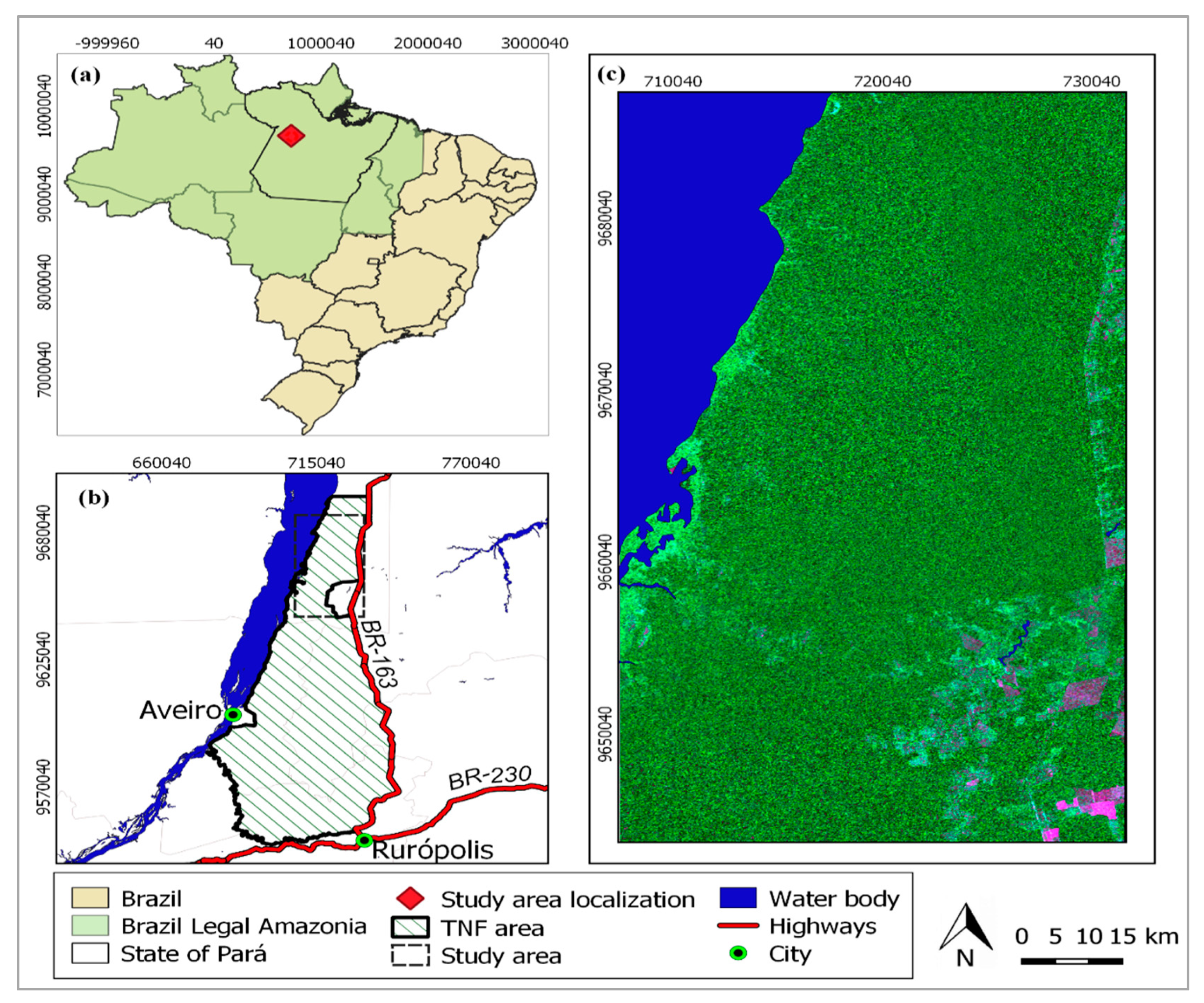
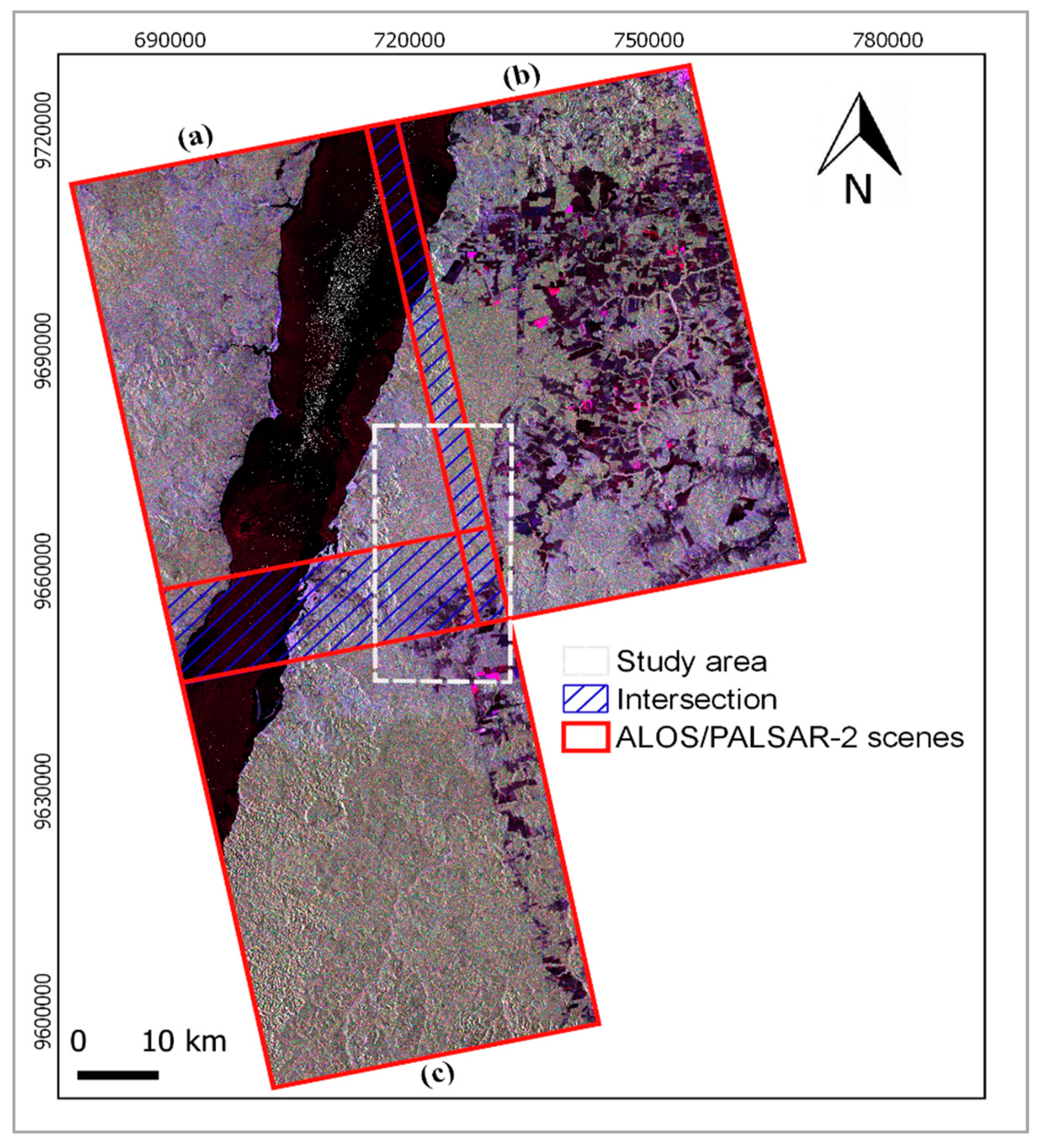
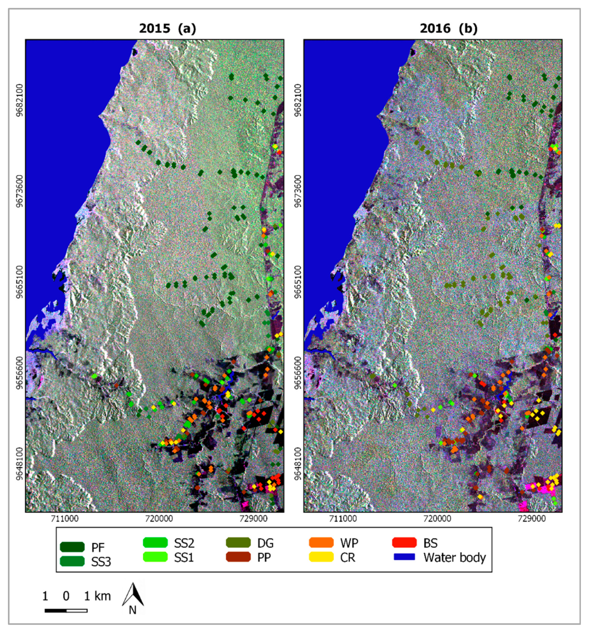
In the southeastern portion of Pará state, we find the Tapajós National Forest (TNF), a federal conservation unit that comprises many of the unique attributes of the Brazilian Amazon, such as well-preserved forested areas with primary forest/old growth forest and forest in different successional stages. Three successional stages are found: advanced secondary succession (SS3); intermediate secondary succession (SS2); and initial secondary succession (SS1). The area is also surrounded by different types of land use. It also faces multi-factor anthropic pressures, illegal logging impacts [23], and historically, the area has suffered from alarming fire spread events [24]. In 2012, TNF lost 17,851 ha of its previous area, due to the Federal Law no. 12.678/2012 that reduced the TNF boundaries, increasing the pressure over considerable primary forest remnants in the excluded zone. Furthermore, amendments to the Brazilian Forest Act promulgated in the same year changed the minimum area requirement that should be maintained as legal reserve (Brazil’s environmental legislation obligates private properties to retain a fixed proportion of their total area with native vegetation, these areas are called “legal reserves”) [25,26]. In this context, studies involving land use and land cover (LULC) classes provide more detailed insights into the analysis of the cause/effect relationships of forest loss, allowing better surveillance and monitoring of conservation units.

Optical satellite remote sensing data has been intensively used for detecting and mapping landscape changes [27]. Such information, in the form of maps, enables the understanding of deforestation patterns [28]. However, the persistent cloud cover in most tropical regions severely restricts the use of optical remote sensing data. On the other hand, synthetic aperture radar (SAR) sensors are almost independent of atmospheric conditions and are sensitive to variations in forest biomass and structure [29,30]. SAR data allow a proper assessment of different LULC classes and forest degradation, especially by fire, even under cloudy conditions, or even under smoke conditions during active fires, as noted in some Amazonia rainforest sites [31,32]. Radar sensors with longer wavelengths, such as the one onboard the Advanced Land Observing Satellite/Phased Array L-band Synthetic Aperture Radar (ALOS/PALSAR) satellite, present higher penetration of transmitted microwave signals into the forest canopy when compared with radar sensors with shorter wavelengths, such as the X-band, TerraSAR/TanDEM-X and Cosmo-SkyMed satellites, or the C-band, RADARSAT-2, and Sentinel-1A/1B satellites [33]. SAR signals at relatively long wavelengths of ALOS/PALSAR can interact with tree stems, branches, trunks, and even ground, depending on the canopy structure [34]. In addition, SAR images obtained in L-band provide better distinction between forest and other LULC classes [31].

The use of ALOS/PALSAR data to monitor forest disturbances and LULC classes has increased in the past years. Pôssa et al. [35] evaluated the potential of full polarimetric ALOS/PALSAR-1 scenes to map LULC in the TNF and surroundings by analyzing interferometric coherence and polarimetric attributes. An association of attributes derived by the Cloude–Pottier decomposition and interferometric coherence showed the best classification results, with an overall accuracy (OA) of 78.8% and Kappa index of 0.72. Pereira et al. [36] also used ALOS/PALSAR-1 image with dual-polarization mode (HH and HV) to evaluate LULC classification in a section of Belterra municipality, Pará state. According to these authors, PALSAR scenes and selected features were not suitable for discrimination of densely forested classes. On the other hand, there was good discrimination among the groups of forested and agro-pastoral classes, as well as among nondensely forested classes, such as pastures, bare soil, and new regeneration. The classification result showed 67.0% for OA, and 0.38 for the Kappa index.

Mermoz and Le Toan [37] used ALOS/PALSAR-1, dual-polarized data to assess rainforest forest disturbances and regrowth in Vietnam, Cambodia, and Laos between 2007 and 2010. The ${\delta }_{HH/HV}^{°}$ ratio showed the best classification results in the time series, with a producer’s accuracy (PA) of 84.7%, and a user’s accuracy (UA) of 96.3%. Martins et al. [38] evaluated the sensitivity of the full polarimetric ALOS/PALSAR-1 to forest degradation caused by fires in the Brazilian Amazon. They used polarimetric and derivate attributes from backscattering coefficients (σ°) to estimate above-ground biomass (AGB), from multiple regression models. The subset formed by anisotropy, double-bounce, orientation angle, volume index, phase difference, and ${\sigma }_{HV}^{°}$ presented the best results. These results showed that the attributes were sensitive to canopy biomass variations due to fire events, but they were not capable of discriminating among intermediate classes. Forests mildly affected by fire had a higher contribution to the scattering in the VV polarization, while forests strongly affected by fire and those with multiple fire events had a larger sensitivity to the HH polarization. The results suggest a greater contribution of horizontally distributed components, such as fallen stems and branches in areas severely affected by fire.

Recent studies focusing on multi-sensor analysis for LULC mapping and change detection in tropical regions [39,40] have used dual-polarimetric ALOS/PALSAR-2 images integrated with Landsat multispectral images. Pavanelli et al. [39] highlighted the SAR potential to discriminate savannah-like vegetation in the Brazilian Amazon, with an improvement in OA of 6% in relation to the classification results obtained only from optical data. De Alban et al. [40], using a similar dataset, assessed the tropical landscapes of southern Myanmar using Random Forest (RF) classifier. They found that SAR-derived texture achieved an OA ranging from 56% to 71%, depending on the dataset used. However, these reported studies rely on low cloud cover conditions during the satellite image acquisition. Hagensieker and Waske [41] highlighted the importance of using SAR images for overcoming such drawbacks in tropical regions. These authors used dual-polarized ALOS/PALSAR-2, RADARSAT-2, and TerraSAR-X images for LULC classification in the Brazilian Amazon, achieving OA of 62% for mono-temporal analysis with ALOS/PALSAR-2 images.

ALOS/PALSAR-2 was launched in 2014 as a successor of ALOS/PALSAR-1 that stopped operating in early 2011. Full-polarimetric images of the new ALOS mission, which includes improved PALSAR-2 sensor with better radiometric and spatial resolutions, have not been tested for LULC classification purposes in the Tapajós region yet. Similarly, this sensor’s potential to discriminate forest in different successional stages and to detect burn scars in forested areas has not yet been evaluated either. These better radiometric quality and higher spatial resolution are expected to increase classification accuracy.

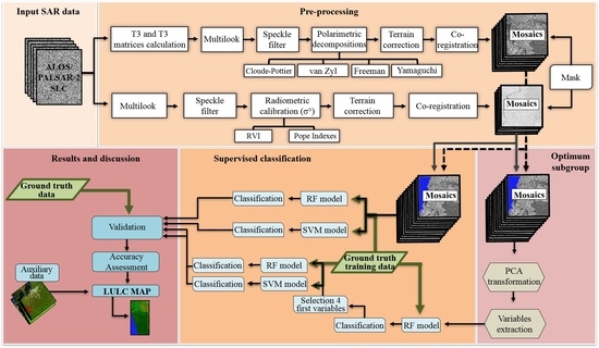
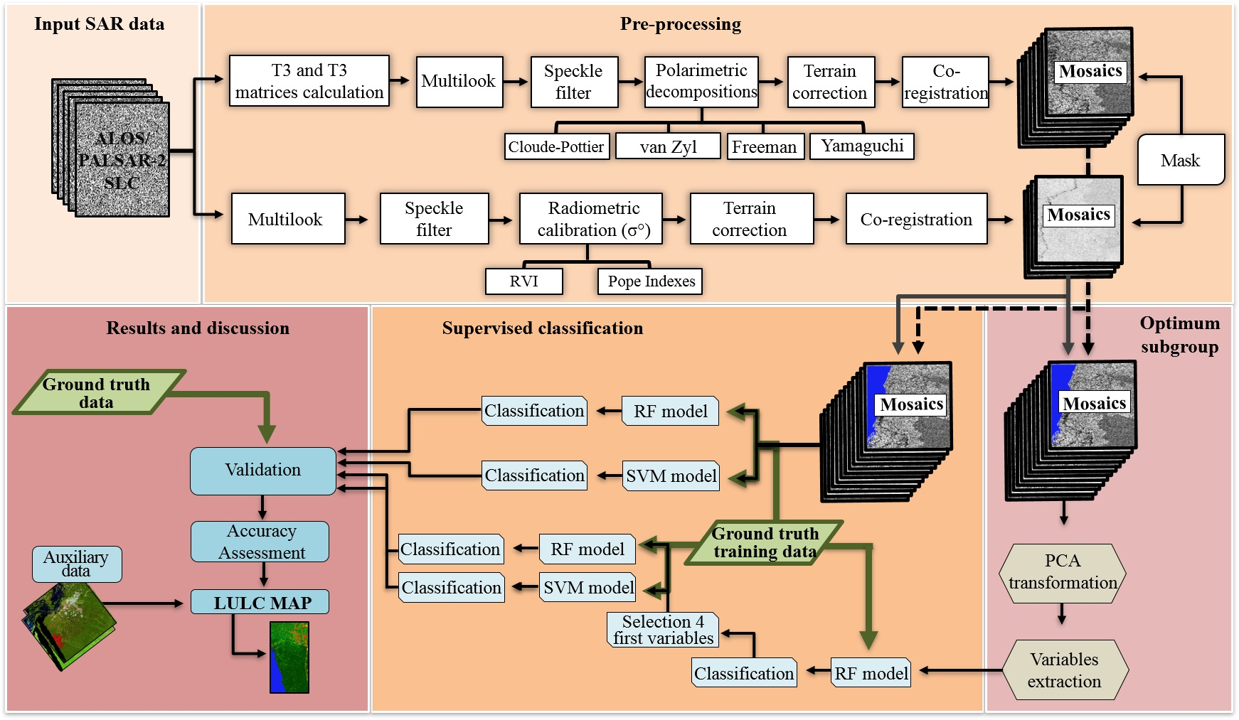
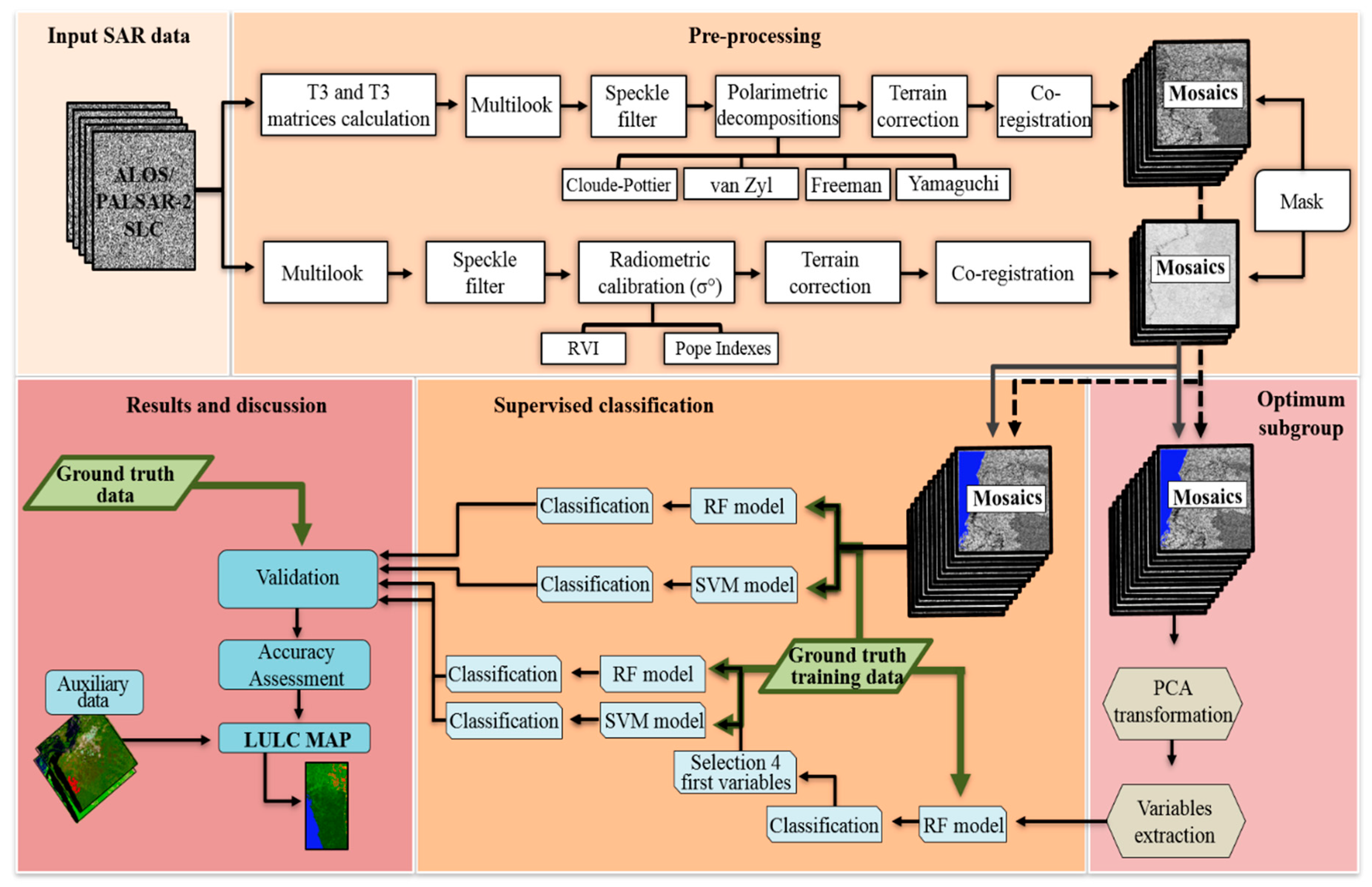
In this study, the specific goals are: (1) to test the potential of ALOS/PALSAR-2 acquired in 2015 and 2016, full-polarimetric images processed by the polarimetric target decomposition techniques to discriminate different LULC classes and to detect forest degradation; (2) to determine the optimum subset of attributes to be used in LULC classifications and degradation forest studies, and (3) to evaluate the performance of both RF and Support Vector Machine (SVM) classification algorithms to discriminate LULC classes and forest degradation over the TNF region.

It is important to highlight that although two dates are available, this study does not aim to quantitatively compare the results of both dates in terms of LULC changes. This is due to the fact that the ALOS/PALSAR-2 images used were acquired in different periods and seasons, with increased effects of seasonality. Additionally, land management practices also vary throughout the year, which can cause substantial errors in any change detection analysis [42,43,44,45].

2. Materials and Methods

2.1. Study Area

The study area is located near the city of Santarém in Pará State, Central Brazilian Amazon, along the BR-163 highway (Cuiabá-Santarém highway) and covers a portion of the TNF and surroundings (eastern side of the national park) (Figure 1). Some settlements, mainly the São Jorge community, are not inside the national park anymore, after the 2012 changes in the TNF boundary. Small-farm settlements are dominant in the São Jorge community with a landscape constituted by well and poorly managed fragments of pasturelands and forest fragments at different stages of succession.

The climate of the region is classified by Köppen as AmW (Monsoon type with short dry season), with an average annual temperature of 25 °C and average relative humidity of 85%. The average annual rainfall is 1909 mm, with a dry season between July and November [46]. The site is situated in a relatively flat area with an elevation between 80 m and 180 m [47,48]. Vegetation in the TNF is formed mainly by dense and open ombrophilous rainforests. These forests are composed of a continuous canopy of perennial trees with heights between 25 m and 30 m and occasional emergent trees that reach up to 50–60 m height [48]. This type of forest has several layers and sublayers under the canopy, including small trees, shrubby, and herbaceous plants. Tall trees are approximately evenly spaced due to the low light penetration into the canopy. There are high amounts of climbing plants, especially epiphytes and lianas, that often hide the outline of the trees [49].

Some areas inside the TNF are allowed to have sustainable selective logging while other areas, under full protection prerogatives, are in the advanced ecological successional stage. Part of the area has been degraded by fire, mainly by fire events that occurred at the end of 2015 and early 2016 [50,51]. Along the BR-163 highway (outside of the park), there are large areas with agricultural activities, cattle ranching, and forest fragments in different succession stages. Growing farming activities near the TNF and reduction of the original TNF area by the Federal Law no. 12.678/2012, have also imposed additional pressures on this conservation unit.

2.2. Field Data

A set of 288 samples were characterized in a field campaign conducted in September 2014 during the dry season. For each sample, representative field photos and geographic coordinates (latitude and longitude), using a Global Positioning System (GPS) receiver (Garmin eTrex10 model), were gathered. The sites were selected based on specific research interests and on previous field campaigns carried out in 2012, 2014, and 2016 [35,48,52,53]. These previous authors have also defined site-specific land cover classes of interest, based on widely used criterion to differentiate succession processes in the Brazilian Amazon as presented by Vieira et al. [54] and Uhl et al. [55], as well as land use adequate to local landscape, presented by Pôssa et al. [35]. The dominant LULC typology for each site was defined as: Primary Forest (PF); Advanced Secondary Succession (SS3); Intermediate Secondary Succession (SS2); Initial Secondary Succession (SS1); Degraded Forest (DG); Poorly Managed Pasture (PP); Well Managed Pasture (WP); Cropland (CR); and Bare Soil and Fallow (BS) (

Table 1. Description of representative land use and land cover (LULC) classes found in the study area.

Initials	LULC Class	Description
PF	Primary Forest	Forests without anthropogenic alterations or with weak or well managed selective logging activities
SS3	Advanced Secondary Succession	>15 years of regeneration
SS2	Intermediate Secondary Succession	5–15 years of regeneration
SS1	Initial Secondary Succession	<5 years of regeneration
DG	Degraded Forest	Forests severely affected by fires and/or unsustainable logging
PP	Poorly Managed Pasture	Pastures with high incidence of shrubs, palms, and trees
WP	Well Managed Pasture	Pastures with low incidence of shrubs and trees
CR	Cropland	Annual crops, mostly soybean, rice, and maize in different phenological stages
BS	Bare Soil/Fallow	Soils prepared for crop planting or temporarily without crop plantation (fallow)

). Another field campaign was conducted in September 2016, where 267 samples were characterized. Most of these sites were the same as visited in 2014. It is important to highlight that although all the field surveys were conducted in a different time to SAR data acquisition, we assume that up to six months’ time difference does not provide significant changes in LULC classes.

A better delineation of the DG class produced by fires was done using the thermal anomalies and fire products from the Moderate Resolution Imaging Spectroradiometer (MODIS) sensor onboard TERRA and AQUA platforms (MOD14 and MYD14, respectively), obtained from the end of 2015 to early 2016. In addition, two Landsat-8 Operational Land Imager (OLI), multispectral images (path/row: 227/62) were used to visually analyze areas of degraded forests mainly by fire, comparing with those classified from ALOS/PALSAR-2 image. The images were obtained from the United States Geological Survey (USGS) website (earth explorer user interface). These orthorectified images have a spatial resolution of 30 m, radiometric resolution of 12 bits, and processing level of 1T. The selected images were obtained on 14 August 2015, which corresponds to the period before the fire events in the Tapajós region, and, from 29 June 2016, which corresponds to the period after the fire.

2.3. ALOS/PALSAR-2 Data and Preprocessing

Figure 2 shows the flowchart of the methodology used to discriminate the land cover, land use, and forest degradation in the TNF region. Our reference dataset consisted of samples obtained in the field campaigns. We used a combination of the reference samples and ALOS/PALSAR-2 full polarimetric images as predictor variables to discriminate the classes in the study area. Description of each step of the methodology is provided in the following subsections.

To cover the entire study area, a mosaic of three ALOS/PALSAR-2 images in polarimetric StripMap-2 (SM2) mode was used for each year (Figure 3). The images were obtained with 1.1 processing level (single look complex data) (

Table 2. Main characteristics of the ascending, full polarimetric ALOS/PALSAR-2 StripMap (SM2) acquisition mode images selected for this study.

Overpass	Range Resolution (m)	Azimuth Resolution (m)	Incidence Angle (degree)	3-Day Accumulated Precipitation (mm) before SAR Overpass
12/28/2014	3.13	2.86	33.86	0.00
04/19/2015	3.21	2.86	33.87	19.87
05/03/2015	3.13	2.86	31.10	10.33
04/17/2016	3.21	2.86	33.87	1.07
05/01/2016	3.13	2.86	31.08	27.17
05/01/2016	3.13	2.86	31.09	27.17

). For each ALOS/PALSAR-2 image, polarimetric scattering matrices and backscattering coefficients (σ°) were generated using the SNAP 7.0 software. A multilook processing was carried out with a window size of 3 pixels × 3 pixels (pixel sizes of 8.5 m by 9.5 m in azimuth and range directions, respectively). To reduce the speckle effect, the matrices were smoothed with the Refined Lee filter [56] (Figure 2). The filter was selected based on the results from previous studies developed in the same study area using ALOS/PALSAR-1 images [35,38,47]. In this study, the following window sizes were tested: 3 × 3, 5 × 5, 7 × 7, and 9 × 9 pixels. The window size of 5 × 5 was selected because it presented a best performance in the reduction of speckle effect and the best preservation of the integrity of spatial information in the SAR image (especially in areas with high landscape fragmentation). This filtering process reduced the speckle effects by 25% according to the Coefficient of Variation (CV) tests.

After filtering, the following polarimetric decompositions were considered: (a) the Cloude–Pottier (CP) technique [57], generating the entropy (H), alpha angle (α), and anisotropy (A) attributes; (b) the van Zyl (VZ) technique [58], generating the surface (VZ_s), double-bounce (VZ_d), and volumetric (VZ_v) scatterings; (c) the Freeman–Durden (FD) technique [59], generating the surface (P_s), double-bounce (P_d), and volumetric (P_v) scattering attributes; and d) the Yamaguchi (YH) technique [60], generating the surface (Y_s), double-bounce (Y_d), volumetric scattering (Yv), and helix scattering (Y_H) attributes (see more details in Appendix A). These polarimetric decompositions were selected in order to test how effective they are for classification purposes. Although the Freeman–Durden and Yamaguchi technique similarly decomposes the polarimetric signal, the fourth additional component of Yamaguchi decomposition (Y_H) could perform well in the discrimination of specific successional forest stages. This component is an improved version of the tree-component Freeman technique [61].

The SAR images were also radiometrically calibrated into σ° whose attributes were used to calculate Radar Vegetation Index (RVI) [62] and the Pope indexes (PI) [63] (Figure 2) of Canopy Structure Index (CSI), Volume Scattering Index (VSI), and Biomass Index (BMI) (see more details in Appendix A). A summary of the attributes is presented in

Table 3. Attributes extracted from the ALOS/PALSAR-2 polarimetric data.

Attributes	Symbol	Description	Source	Equation
Entropy	H	Number of dominant scattering mechanisms	Cloude and Pottier [57]	$\mathrm{H}=-{\displaystyle \sum _{\mathrm{i}=1}^3}{\mathsf{\rho }}_{\mathrm{i}}{\log }_3({\mathsf{\rho }}_{\mathrm{i}});{\mathsf{\rho }}_{\mathrm{i}}=\frac{{\mathsf{\lambda }}_{\mathrm{i}}}{{\sum }_{\mathrm{j}=1}^3{\mathsf{\lambda }}_{\mathrm{j}}}$
Mean alpha angle	${\displaystyle \overline{\mathsf{\alpha }}}$	Dominant scattering mechanism		${\displaystyle \overline{\mathsf{\alpha }}}={\displaystyle \sum _{\mathrm{i}=1}}{\mathsf{\rho }}_{\mathrm{i}}{\mathsf{\alpha }}_{\mathrm{i}}$
Anisotropy	A	Measures the relative importance of the second and third scattering types		$\mathrm{A}=\frac{{\mathsf{\lambda }}_2-{\mathsf{\lambda }}_3}{{\mathsf{\lambda }}_2+{\mathsf{\lambda }}_3}$
Surface scattering	VZs	Portion of surface scattering	van Zyl [58]	${\mathrm{P}}_{\mathrm{odd}}={\mathsf{\lambda }}_{\mathrm{odd}}+\left|C_{odd}\right|$
Double-bounce	VZd	Portion of double-bounce scattering		${\mathrm{P}}_{\mathrm{even}}={\mathsf{\lambda }}_{even}+\left|C_{even}\right|$
Volumetric scattering	VZv	Portion of volumetric scattering		${\mathrm{P}}_{\mathrm{canopy}}=a\left[C_{canopy}\right]$
Surface scattering	Ps	Portion of surface scattering	Freeman and Durden [59]	${\mathrm{P}}_{\mathrm{s}}={\mathrm{f}}_{\mathrm{s}}\left(1+\left|\mathsf{\beta }\right|²\right)$
Double-bounce	Pd	Modeled from two orthogonal surfaces		${\mathrm{P}}_{\mathrm{d}}={\mathrm{f}}_{\mathrm{d}}\left(1+\left|\mathsf{\alpha }\right|²\right)$
Volumetric scattering	Pv	Modeled from a cloud of fine cylindrical scatterers randomly distributed		${\mathrm{P}}_{\mathrm{v}}=\frac{8_{\mathrm{fv}}}{3}$
Surface scattering	Ys	Portion of surface scattering	Yamaguchi et al. [60]	${\mathrm{P}}_{\mathrm{s}}={\mathrm{f}}_{\mathrm{s}}\left(1+\left|\mathsf{\beta }\right|²\right)$
Double-bounce	Yd	Modeled from two orthogonal surfaces		${\mathrm{P}}_{\mathrm{d}}={\mathrm{f}}_{\mathrm{d}}\left(1+\left|\mathsf{\alpha }\right|²\right)$
Volumetric scattering	Yv	Modeled from a cloud of very fine and cylindrical scatterers randomly distributed		${\mathrm{P}}_{\mathrm{v}}={\mathrm{f}}_{\mathrm{s}}$
Helix scattering	YH	Helix shape scattering		${\mathrm{P}}_{\mathrm{c}}={\mathrm{f}}_{\mathrm{c}}$
Radar Vegetation Index	RVI	Parameter sensitive to the biomass level	Kim and van Zyl [62]	$\mathrm{RVI}=\frac{8{\mathsf{\sigma }}_{\mathrm{HV}}}{{\mathsf{\sigma }}_{\mathrm{HH}}+{\mathsf{\sigma }}_{\mathrm{VV}}+2{\mathsf{\sigma }}_{\mathrm{HV}}}$
Canopy Structure Index	CSI	Parameter that measures the relative importance of horizontal versus vertical structure in the vegetation	Pope et al. [63]	$\mathrm{CSI}= \frac{{{\mathsf{\sigma }}^{°}}_{\mathrm{VV}}}{{{\mathsf{\sigma }}^{°}}_{\mathrm{VV}} {{\mathsf{\sigma }}^{°}}_{\mathrm{HH}}}$
Volume Scattering Index	VSI	Parameter indicating canopy density or thickness		$\mathrm{VSI}=\frac{{{\mathsf{\sigma }}^{°}}_{\mathrm{HV}}}{{{\mathsf{\sigma }}^{°}}_{\mathrm{HV}} +\mathrm{BMI}}$
Biomass Index	BMI	Indicator parameter of the relative amount of woody compared to leafy biomass		$\mathrm{BMI}= \frac{{{\mathsf{\sigma }}^{°}}_{\mathrm{HH}} + {{\mathsf{\sigma }}^{°}}_{\mathrm{VV}}}{2}$

. All images were individually processed. Images were geometrically corrected using a 30 m digital elevation model (DEM) derived from the Shuttle Radar Topography Mission (SRTM). The images were coregistered to generate the mosaics of each year.

For this study, we generated only the variables of Table 3 because they had shown the best performances between all the SAR attributes generated in other studies for the same region in Amazon considering some similar classes but with different SAR data and methodological approaches [35,47,51].

2.4. Water Body Masking

Bare soils and water bodies, when interacting with electromagnetic energy, tend to produce relatively low levels of surface scattering, mainly at the L-band wavelengths. Similar backscattering of these targets can produce poor separability classes, resulting in misclassifications of both targets [64], so that we used a water body mask. To create the mask, we used the vector-based Main Rivers file available in the National Water Agency (ANA) database [65]. This product was mapped on 1:1,000,000 scale, and the drainage area was extracted from SRTM data. In the mask building process, we clipped the water bodies found in the study area and assigned them a value equal to zero. The remaining areas assigned a value equal to one, producing a binary mask: water/nonwater. During this process the areas with a value equal to one were considered in the calculation, whereas the areas with a value equal to zero were discarded [66]. Then, the mask was applied to all polarimetric decompositions and to the full-pol images calibrated into σ°.

2.5. LULC Classes

In order to classify the LULC classes, we used reference samples obtained in the field campaigns, as previously described in Section 2.2. Each field sample was georeferenced based on the GPS coordinates. To reduce the speckle effect that is inherent to SAR data, each sampling point was converted to polygons through the buffer function available in the QGIS software. After some tests, the buffer zone of 24.75 m was selected, which is equivalent to an area of ~1800 m² for each polygon. The criterion used here was the visual analysis of the sample spatial distribution in our study area. High spatial resolution images from Google Earth™ platform (12/30/2014 and 30/12/2015) were used to support the inspection of each polygon.

Figure 4 shows the location of the polygon samples over nine LULC classes found in the study area. The representativeness of the samples in terms of total number of polygons, pixels, and areas (in hectares) for each year is shown in

Table 4. Number of polygons, pixels, and corresponding areas per land use and land cover (LULC) class that was considered in Random Forest and Support Vector Machine classification processes involving ALOS/PALSAR-2 images from 2015 and 2016. For LULC class identification, see Table 1.

Classes	2015			2016
	Polygon	Pixel	Area (ha)	Polygon	Pixel	Area (ha)
PF	116	1044	20.88	47	423	8.46
SS3	22	198	3.96	5	45	0.90
SS2	37	333	6.66	11	99	1.98
SS1	09	81	1.62	18	162	3.24
DG	09	81	1.62	77	693	13.86
PP	26	234	4.68	40	360	7.20
WP	30	270	5.40	28	252	5.04
CR	21	189	3.78	31	279	5.58
BS	18	162	3.24	10	90	1.80
Total	288	2592	51.84	267	2403	48.06

. The samples were used as ground truth in the RF and SVM classifications.

2.6. Optimum Subgroup Definition

To select the variables that better discriminate the LULC classes, subgroups of different polarimetric attributes and backscattering coefficients were formed and were named as optimum subgroups. To obtain these subgroups, we carried out for 2015 and 2016 separately all steps presented below. The selection of these optimum subgroups, the Principal Component Analysis (PCA), was initially applied in order to reduce the dimensionality of the datasets (see Section 2.6.1). Sequentially, the most important variables derived from the PCA were selected and used as input data set in the RF classification (see Section 2.7). To compose the training and validation set of the model, we selected 75% of samples for training and 25% for validation. During the RF classification process, the algorithm calculated the features based on the importance of each variable. In this study, we selected the first four most important variables. The variable importance shows the interaction between the variables and hierarchizes them within a level of contribution and importance for the classification [67]. The same first four variables based on variable importance selected in RF were also used for SVM classifier. It is important to highlight that, as well as the PCA and the classification in the RF for each year that were performed separately; the SVM classification also was carried out for each year separately. More details on PCA and RF and SVM classification steps are described in the next subsections.

Principal Component Analysis

PCA is considered an important statistical technique that enables reducing the data dimensionality [68,69], extracting the components accounting for as much variance as possible through a linear transformation [70]. In this context, to form an optimum subgroup for the LULC classification, we applied the PCA technique to reduce the number of variables from the polarimetric decompositions and σ° data sets. We used the first principal component (PC1) and the second principal component (PC2) only to aggregate information that was more relevant to the classification process. For these two principal components, we selected only those variables whose contributions were higher than 5%. In addition, similar variables derived from different polarimetric decompositions were excluded, for example, double-bounce scatterings derived from van Zyl, Freeman–Durden, and Yamaguchi decompositions. A total of 17 input parameters (13 from polarimetric decompositions and 4 from σ°) were selected, being 9 variables from 2015 and 8 variables from 2016 images. The PCA technique was performed in the R 1.7.3 software [71].

2.7. Classification and Evaluation

All seven groups of attributes (CP, VZ, FD, and YH polarimetric decompositions, RVI, PI backscattering indexes, and optimum subgroups) from both years were used as input data in RF and SVM supervised classification algorithms (

Table 5. Performance of the optimum subgroup of attributes in Random Forest (RF) and Support Vector Machine (SVM) classifiers. Attribute identification: H (entropy), α (alpha angle), and A (anisotropy) from Cloude–Pottier; P_v (volumetric scattering), and P_s (surface scattering) from Freeman–Durden; VZ_d (double-bounce scattering) from van Zyl, and BMI (Biomass Index) from Pope indexes. Details of the SAR derived attributes are presented in Table 3.

2015
Optimum Subgroup Attributes	Classifier	OA (%)	CI. 95%	Kappa	Processing Time (s)
α, A, Pv, VZd	RF	75.4	71.9–78.7	0.68	686.40
	SVM	70.9	67.2–74.4	0.62	1080.00
2016
H, A, Ps, BMI	RF	79.9	76.4–83.0	0.76	889.16
	SVM	76.8	73.2–80.2	0.71	867.60

and

Table 6. Performance of different subsets of attributes for LULC classes classified by Random Forest (RF) and Support Vector Machine (SVM) algorithms.

2015
Attribute Groups	Classifier	OA (%)	CI. 95%	Kappa	Processing Time (s)
CP (H, α, A)	RF	60.0	56.0–64.0	0.46	564.50
	SVM	64.6	60.7–68.3	0.50	783.89
VZ (VZs, VZd, VZv)	RF	70.7	67.0–74.2	0.61	509.80
	SVM	69.8	66.0–73.3	0.59	629.80
FD (Ps, Pd, Pv)	RF	72.8	69.1–76.2	0.64	503.84
	SVM	71.3	67.7–74.8	0.63	690.91
YH (Ys, Yd, Yv, YH)	RF	76.9	73.4–80.1	0.70	811.48
	SVM	69.8	66.0–73.3	0.60	1246.85
RVI	RF	40.4	36.5–44.3	0.23	316.88
	SVM	46.2	42.3–50.2	0.23	755.76
PI (CSI, VSI, BMI)	RF	64.0	60.2–67.8	0.52	564.93
	SVM	62.5	58.6–66.2	0.49	887.64
2016
Attribute Groups	Classifier	OA (%)	CI. 95%	Kappa	Processing Time (s)
CP (H, α, A)	RF	72.9	69.1–76.4	0.67	696.92
	SVM	72.9	69.1–76.4	0.67	885.80
VZ (VZs, VZd, VZv)	RF	79.2	75.7–82.4	0.74	527.91
	SVM	78.2	74.6–81.4	0.74	741.98
FD (Ps, Pd, Pv)	RF	80.2	76.7–83.4	0.76	589.55
	SVM	77.0	73.3–80.3	0.72	623.44
YH (Ys, Yd, Yv, YH)	RF	83.3	80.0–86.2	0.80	658.07
	SVM	78.7	75.1–81.9	0.74	957.32
RVI	RF	32.2	28.5–36.2	0.18	343.07
	SVM	39.8	35.8–43.8	0.22	864.16
PI (CSI, VSI, BMI)	RF	56.3	52.2–60.4	0.46	578.22
	SVM	51.0	46.9–55.	0.39	906.22

CP: Cloude–Pottier decomposition; VZ: van Zyl decomposition; FD: Freeman–Durden decomposition; YH: Yamaguchi decomposition; RVI Index and; PI: Pope Index. Details of the SAR derived attributes are presented in Table 3.

). These algorithms were implemented in R software and received increasing attention, due to their accurate classification results and their processing performance [72,73].

RF and SVM support data with different statistical distributions and can support several input parameters, providing consistent results [67,74]. In SAR data applications, they are less affected by noisy data, showing good classification results involving LULC dynamics in forests [75,76,77]. RF algorithm consists of an ensemble of decision trees, where each tree contributes with just one vote for the assignment of the most frequent class to the input data set [78]. The final classification result is determined by the highest number of votes of all forest trees. The algorithm uses bagging (bootstrap) and random samples from training sets for tree building with replacement in the original training set [79,80]. The samples that are excluded from the bootstrap are called out-of-bag (OOB) samples. The OOB samples help to evaluate misclassification error and to estimate variable importance [78]. To estimate the importance of each predictor variable in the RF model, we used the mean decrease in accuracy (MDA) method. This method is calculated by the normalized difference between OOB accuracy of the original observations and the randomly permuted variables [81]. Higher scores of MDA indicate that variables are important predictors in the classification. There are two essential parameters in the RF model: the number of input variables in the random subset of variables at each node and the number of trees. The grown trees are not pruned to ensure lower diversity among individual trees and obtain low biased trees. RF can still measure the relative importance of each variable within the model. Each variable is ranked according to its contribution to the classification accuracy.

In this study, to build the RF model, 75% of samples were used for training, and 25% for validation. A default value of the number of variables was adopted, which corresponds to the square root of the total number of input variables [78]. A total of 500 trees was considered. Each polarimetric decomposition and backscattering index was classified individually, following the parameter value mentioned above. Considering the optimum subgroup, the variables selected in PC1 and PC2 for each year were initially used as input data in the RF algorithm to perform the 2015 and 2016 classifications separately. Subsequently, these same variables were classified, and the variable importance of each one was calculated during the RF classification process. For each year, the first four variables that showed the highest contribution and importance for classifications were selected. In the second step, only these first four selected variables for each year were used for classifications, and their results, respectively, attributed to the optimal subgroup, 2015 and 2016.

The SVM algorithm is based on decision planes that determine decision boundaries in input space or high dimensional feature space [82]. An optimal hyperplane is defined as the linear decision function with the best separation among different training classes in order to maximize the distance among them [83]. The distance between the decision boundary and the closest data point (training data) determines the margin of the classifier. These borderline samples are called support vectors and correspond to the critical elements of the training samples, as they delimit the decision surface [84]. When the data are not linearly separable, which is a common case in the real world, the SVM algorithm uses kernel functions. The original input space is mapped in a higher dimensional feature space, allowing the adjustment of the linear hyperplane and improving the linear separability [85]. The most common kernel functions are linear, polynomial, sigmoid, and radial basis function (RBF).

In this study, to build the SVM model, 75% of samples for training, and 25% for validation were also used. The selected kernel was the RBF, making it necessary to adjust cost (C) and gamma (γ) parameters. C parameter is known as a regularization term that controls the tradeoff between maximization of the margin width and the fitting of the training data set as well as the width γ of the RBF kernel [86]. In order to find the optimum C and γ parameters, we applied the cross-validation method. This method allows obtaining an error estimate in the data sets, randomizing them before building the splits of support vectors [87]. To find the average error, we used 10-fold cross-validation using the training set and the best parameter combinations.

The processing times (training time plus classification time, unit in s) for RF and SVM were also recorded for the purpose of analyzing whether the different polarimetric decompositions and backscatter coefficients presented different runtime performances in different classification algorithms. The computer processor used in the classification step was equipped with Intel^® Core™ i5 2450 CPU, 2.50 GHz, and 6.0 GB usable RAM.

The classification results from both years were analyzed through the Kappa index, OA, and the confidence interval at the significance level of 95% (CI.95%), from RF and SVM classifications. For the best classification results, we also calculated the producer’s accuracy and user’s accuracy as well as F1-scores.

3. Results

3.1. Optimum Subgroup Classification

In order to compose the optimum subset, we initially selected the most important variables derived from PC1 and PC2. For 2015, the variations explained by PC1 and PC2 were 51.3% and 13.0%, respectively (total accumulated variance of 64.3%). In 2016, the variations in PC1 and PC2 were 50.5% and 17.1%, respectively (total accumulated variance of 67.6%). Figure 5 shows the percentage of each variable contribution for PC1 and PC2. These variables are considered the most important ones among all analyzed for 2015 and 2016. We highlight being for VZ_d variable, which presented the highest contribution (23.3%) for 2015. For 2016, the Y_d variable showed the highest contribution (25.3%).

It is important to mention that the principal components of each year are formed by different variables, as shown in Figure 5. The distinct performance between 2015 and 2016, with different percentages of each variable contribution, may occur because: (a) some classes selected in this study presented high temporal and spatial dynamics (mainly PP, WP, CR, and BS). Such dynamics were also clearly observed in the DG class, which in 2016 showed high dynamics when compared with 2015, where the land cover was degraded by fire; (b) the acquisition of ALOS/PALSAR-2 images at different times of the year can influence the backscattering of the targets due to seasonal characteristics; and (c) the precipitation in the study area during some of the SAR acquisitions (Table 2) can directly influence the amount of moisture in the dielectric properties of materials and their SAR backscatter [88].

Afterward, the variables presented in Figure 5 for 2015 were used as input data in the RF algorithm to classify the LULC classes for 2015. The four first variables for 2015 were: P_v, α, VZ_d, and A (Figure 6). In the same way, the variables obtained for 2016 (Figure 5) were used in RF classification for 2016. The four first variables for 2016 were: H, BMI, P_s, and A. Those aforementioned variables proved to be the most important in predicting to discriminate different forest types, forest degradation, and land use classes (Figure 6).

The four most important variables of each year were again classified separately by the RF algorithm. These same variables were also classified separately by the SVM algorithm. Table 5 shows the OA, CI. 95%, Kappa index, and processing time for the optimum subgroups classified by the RF and SVM algorithms for each year.

As can be observed in Table 5, RF and SVM demonstrated their capabilities to classify LULC classes. The best OA and Kappa indices were exhibited by RF, with an OA of 75.4% and 79.9%, and Kappa index of 0.68 and 0.76, for 2015 and 2016, respectively. The RF processing for 2015, was 393.6 s faster than that of the SVM, while for 2016, the SVM was 21.6 s faster than that of RF.

3.2. LULC Classification

Table 6 shows the classification results obtained for different decompositions and σ° for the years of 2015 and 2016, based on the performance of RF and SVM classification algorithms. The values obtained for OA, CI. 95%, Kappa index, and processing time were evaluated. In terms of OA (≥70%) and Kappa index (≥0.70), we can highlight, in 2015, YH polarimetric decomposition and, in 2016 VZ, FD, and YH decompositions. The highest values of OA and Kappa index were obtained by the RF algorithm for the YH decomposition in 2015 and 2016, respectively, with an OA of 76.9% and 83.3%, and Kappa index of 0.70 and 0.80. However, the time spent during the classification process was also one of the highest (≥10 min). The greater number of components of these groups (four components in each group) in relation to the other groups of polarimetric decompositions and backscattering coefficients investigated possibly impacted on the processing time of the classification step. Concerning the performance of RF and SVM and considering the OA and Kappa index criteria, the RF algorithm showed the best classification results for 2015 and 2016. Except for RVI classification, SVM exhibited the best results (Table 6).

Figure 7 shows the performance of RF and SVM classifiers in relation to the OA and processing time of the polarimetric decompositions, σ°, and optimum subgroup. RF exhibited superior performances for the groups of attributes investigated in both years. On average, for 2015, SVM algorithm demanded more than 58% of the classification time in relation to RF and more than 46% for 2016.

In summary, for 2015, YH decomposition presented an improvement of 16.7% for OA and 23.9% for Kappa index, with an additional processing time of more than 246 seconds, when compared to CP decomposition; an increase of 6.1% for OA and 8.7% for Kappa index, with an additional processing time of more than 301.7 s, when compared with VZ decomposition; and 4.1% for OA, 6.1% for Kappa index and additional processing time of 307.6 seconds, when compared with FD decomposition. Concerning PI index, YH decomposition showed an increase of 12.8% for OA, 18.4% for Kappa index, and additional processing time of 246.6 seconds. The gains in relation to RVI were 36.5% for OA and 46.8% for Kappa index. Here, we found the largest differences, indicating that RVI had the worst classification performance. On the other hand, RVI processing time was 494.6 seconds faster than that of YH decomposition. The smallest difference in performance was observed with the optimum subset (α, A, P_v, and VZ_d), with increments of 1.4% for OA, 2.3% for Kappa index, and 125.1 seconds in processing time than that of the optimum subgroup (Table 5 and Table 6 and Figure 7).

In 2016, YH decomposition also showed an increase of 10.4% for OA and 12.9% for Kappa index, with a processing time shorter than 38.8 s, when compared with that of CP classification; 4.1% for OA, 5.3% for Kappa index, and 130.2 s slower than that of VZ decomposition; 27.0% for OA and 33.6% for Kappa index, with a processing time longer than 79.9 s, when compared to that of PI index; 7.7% for OA and 10.2% for Kappa index, with a processing time shorter than 231.1 s in relation to that of the optimum subset (H, A, P_s, and BMI). RVI for 2016 also showed the worst classification performance when compared with that of YH decomposition, with an increase YH of 51.0% for OA and of 61.8% for Kappa index. However, YH was around 315.0 s slower in the processing time. In relation to FD decomposition, YH decomposition showed an increase of 3.1% for OA and of 3.6% for Kappa index, with a processing time higher than 68.5 s, indicating the smallest performance difference among the decompositions (Table 5 and Table 6 and Figure 7).

Based on the values of the parameters shown in Table 5 and Table 6, and aiming to obtain the attributes with the greatest potential to discriminate LULC classes, we selected YH decomposition classified by the RF algorithm considering both years (2015 and 2016).

According to the classification results from YH decomposition for 2015 (Figure 8), among the classes with more dense forest structures investigated, we highlighted the results for the PF class, with a PA of 93.4%, a UA of 81.5%, and a F1-score of 0.87, followed by SS2 class, with PA of 68.2%, UA of 64.4%, and F1-score of 0.66. The highest misclassification was observed for the SS3 class, being misclassified as PF and SS2. The SS3 presented PA of 17.8%, UA of 44.4%, and F1-score of 0.25. The DG class showed PA of 41.2%, UA of 53.8, and F1-score of 0.47 (Figure 8).

Concerning the classes with less vegetation coverage, the best results (PA and UA > 74.0%, and F1-score ≥ 0.77) were found for PP, WP, and BS. On the other hand, CR showed the highest misclassification, with PA of 55.0%, UA of 71.0%, and F1-score of 0.62 (Figure 8). According to YH classification results for 2016 (Figure 9), among the investigated classes that presented a dense forest structure, PF exhibited one of the best accuracy results, with PA of 96.8%, UA of 78.3%, and F1-score of 0.87, followed by the DG class, with PA of 90.1%, UA of 91.7%, and F1-score of 0.91. SS1 showed adequate accuracy, with PA of 71.8%, UA of 63.6%, and F1-score of 0.67. As observed in 2015, SS3 class also showed the highest misclassification, especially in terms of the PA. Around 78.6% of the samples were misclassified and the main misclassification was associated with PF and SS2 classes.

The classes with low levels of vegetation (PP, WP, CR, and BS) showed adequate accuracy (PA and UA > 77.0%, F1-score ≥ 0.78) (Figure 9). The obtained results demonstrated high reliability for each discriminated class, as well as high sensitivity of the classifier to correctly distinguish these classes from the others.

The LULC and forest degradation classification for 2015 and 2016 were produced using the Y_s, Y_d, Y_v, and Y_H attributes from the YH decomposition (Figure 10). The subsets in Figure 11b,c emphasize the areas with the most predominant of land use types in the study area. PP, WP, CR, and BS exhibited high dynamics in terms of areas occupied between 2015 and 2016. Concerning land cover classes (Figure 12), between 2015 and 2016, the main changes observed are related to an increase of areas occupied by DG and a reduction of areas occupied mostly by primary forest and secondary succession classes, where part of the TNF and surroundings has been degraded by fire, because of the occurrence of forest fires events at the end of 2015 and the beginning of 2016.

The changes that occurred in LULC and forest degradation between 2015 and 2016 are only based on qualitative analysis (i.e., a visual analysis) of the YH decomposition classification results, which are clearly noticeable in Figure 10, Figure 11 and Figure 12. A detailed analysis to quantify the losses and gains requires additional change detection techniques that are suggested for future studies. In addition, some thematic classes in the study area such as the cropland, well managed pasture, and bare soil, show high dynamics over the year, which could introduce false changes.

4. Discussion

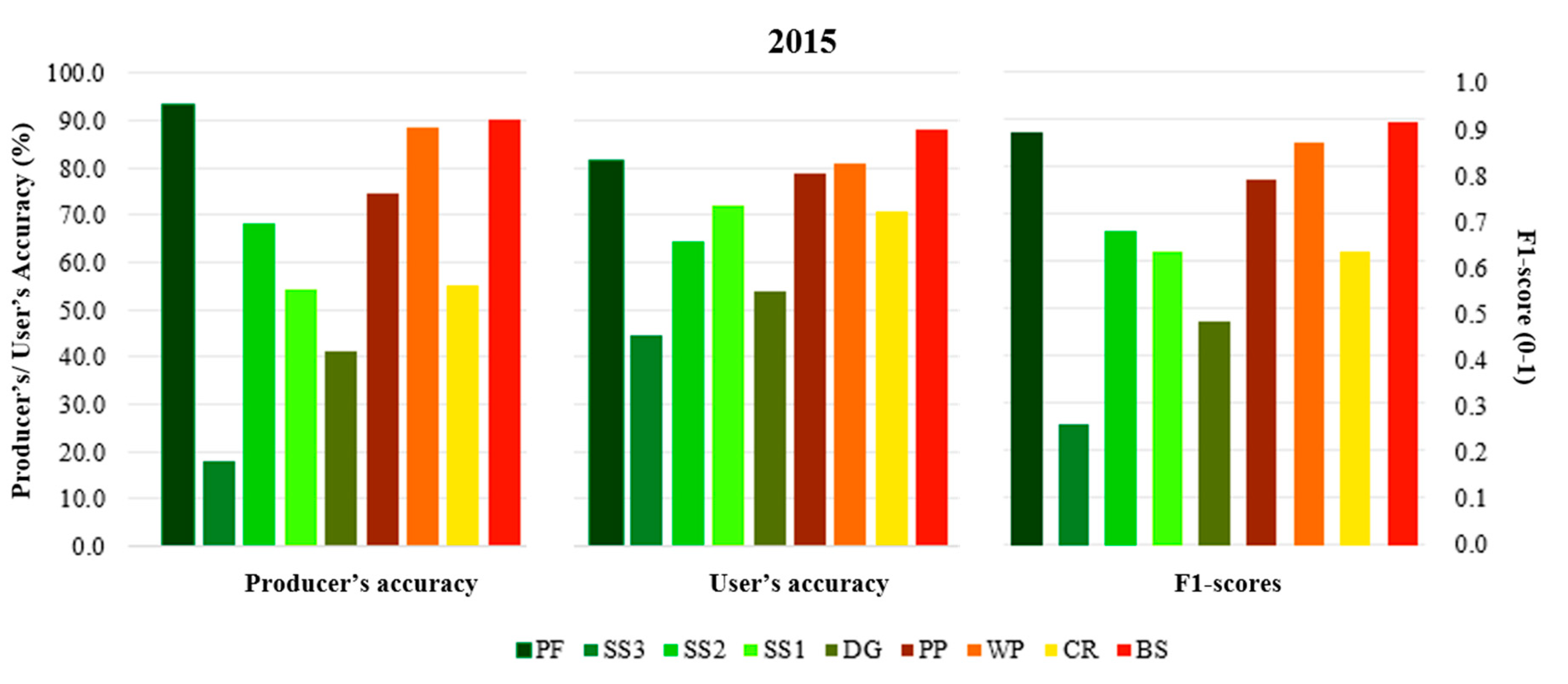
The attributes extracted from the YH decomposition showed the best classification results (Table 5), demonstrating an adequate capability to discriminate different land use types, forest degradation, and land cover classes. The potential to discriminate classes with low levels of vegetation coverage (PP, WP, CR, and BS) was highlighted (Figure 8 and Figure 9). The only exception occurs for the CR class, with PA of 55.0% in 2015 formed by crops with different phenological stages. This class showed the lowest classification performance and was therefore an exception. Classes with low vegetation coverage levels, like CR, can be misclassified due to the flat surfaces that show low levels of backscattering of transmitted signals in L-band, consequently, they cannot be easily distinguished [89]. In addition, some agricultural crops in more advanced stages of development can be easily distinguished from flat surfaces, as mature crops cause more volume scattering.

Some misclassifications that occurred in PP and WP classes can be explained by the presence of inajás (Attalea maripa) and babaçus (Attalea speciosa) [35]. They are pioneer trees species sparsely distributed in both poorly and well managed pastures. The structure of these tree species may cause certain confusion during the classification process, mainly when associated with other forested classes.

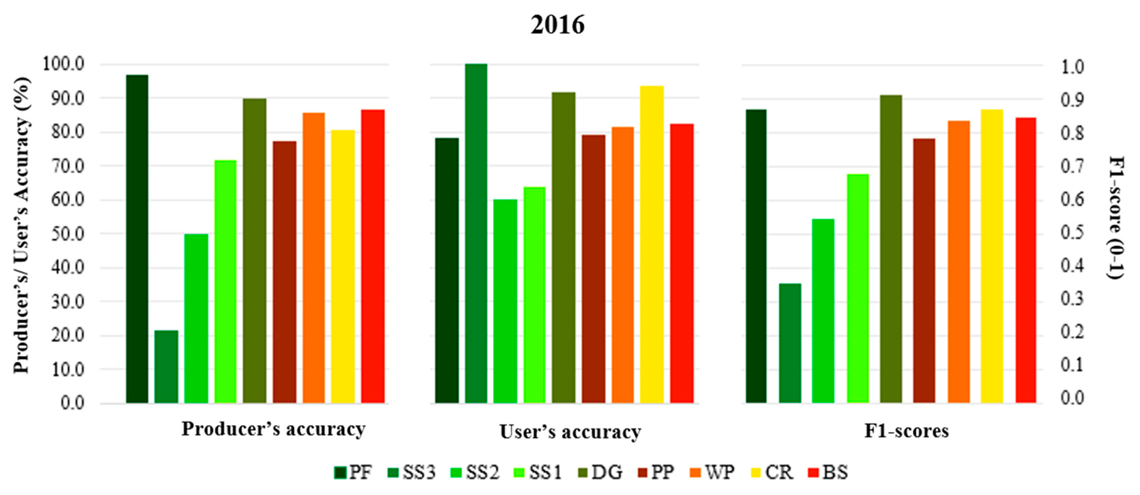
Concerning classes that present a dense forest structure, the PF was the class that exhibited the highest classification results in 2015 and 2016 (Figure 8 and Figure 9), highlighting the great capability of YH decomposition to discriminate primary forest in rainforest environments. However, these attributes were not effective in discriminating SS3 class, especially the misclassification associated with the PA in both years. SS2 also showed intermediate values of PA and UA in both years. Misclassifications between SS2 and SS3 probably occurred due to similarities in their respective structural physiognomic characteristics and the high levels of regenerative development. SS1 also showed intermediate accuracies in both years. In this ecological successional stage, the forest class structure is composed predominantly of only one homogeneous superior stratum and one inferior stratum. The latter is composed of regeneration in its initial succession stages, which are arranged in an irregular form and dispersed in the environment, being influenced mainly by the distribution of pioneer species. Such condition probably was responsible for the misclassification to SS2 and PP classes.

DG classification results showed different behaviors in 2015 and 2016: PA and UA ≥ 53.8%, and F1-score of 0.47, in 2015; and, PA and UA > 90.0% and F1-score of 0.91 in 2016. This difference can be associated with the total number of samples: total of 81 pixels in 2015 and 693 pixels in 2016 (Table 4). In addition, the degraded forest samples collected during the field campaign in 2015 correspond to forests severely affected by fires and by unsustainable logging, while the samples collected in 2016 corresponded mostly to forests severely affected by fires. 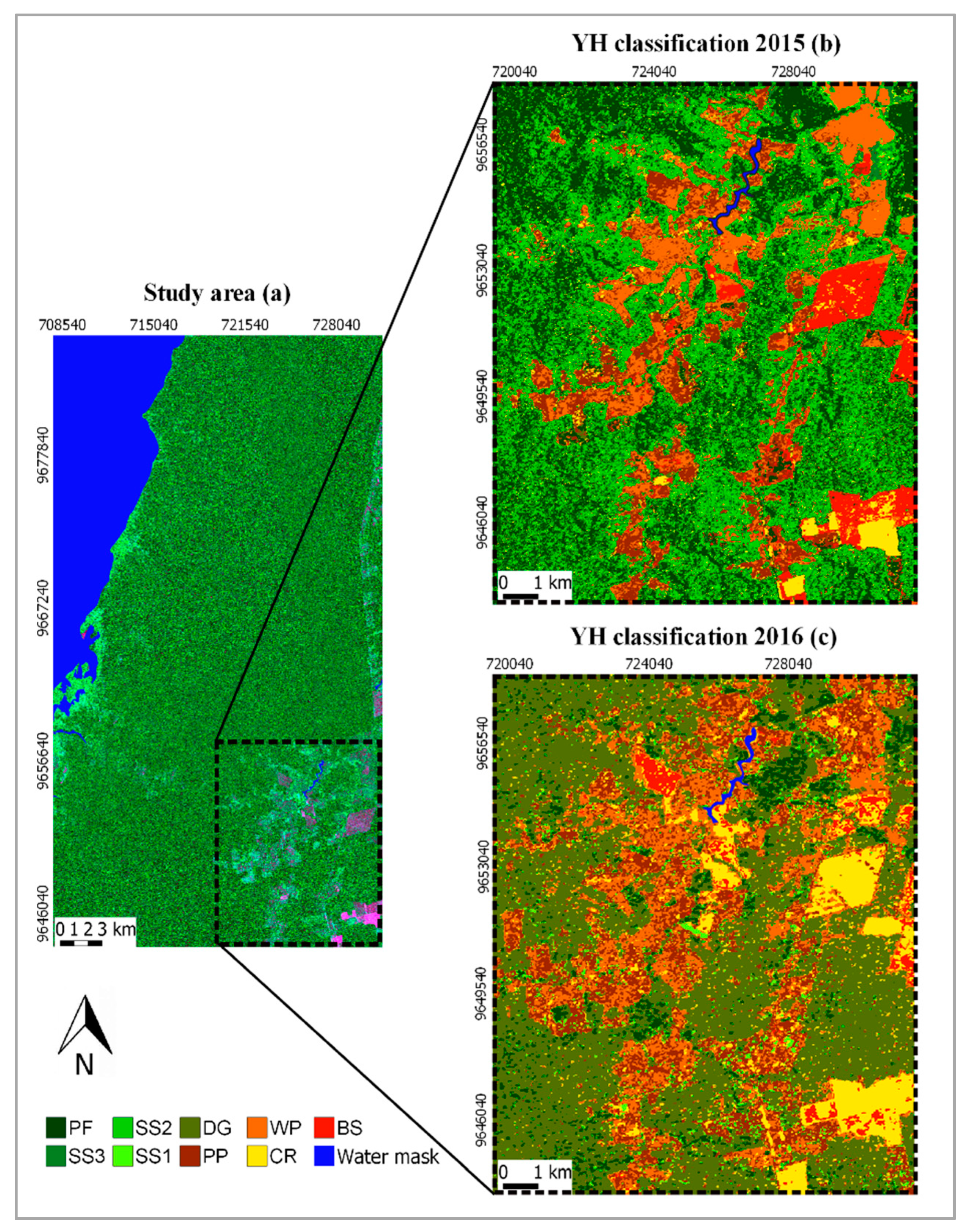In this context, the most homogeneous samples in the DG class were in 2016, which consequently may have contributed to reach better results, demonstrating the capability of the YH attributes to classify forest degradation, mostly degraded by fire (Figure 12).

In general, the intermediate values of accuracy for SS2 and SS1, and the lowest values of accuracy obtained for SS3 in both years, demonstrate that the YH decomposition has a greater capacity to discriminate ecological succession classes from those with less vegetation coverage, despite its poor ability in distinguishing among classes of different ecological succession and disturbance stages, with the exception of PF class. Ullmann et al. [90] examined the scattering characteristics from polarimetric data obtained at X-, C-, and L-band in a tundra-dominant ecosystem and found that L-band data were more appropriate to differentiate classes with low levels of vegetation cover. Pavanelli et al. [39] integrated data from Landsat-8/OLI and ALOS/PALSAR-2 satellites and classified them in the RF algorithm, to map the LULC classes in a fragment located in the northern part of the Brazilian Amazon. They found that ALOS/PALSAR-2 data’s most important contribution was the possibility to discriminate classes with low levels of biomass (grasslands and wooded savanna).

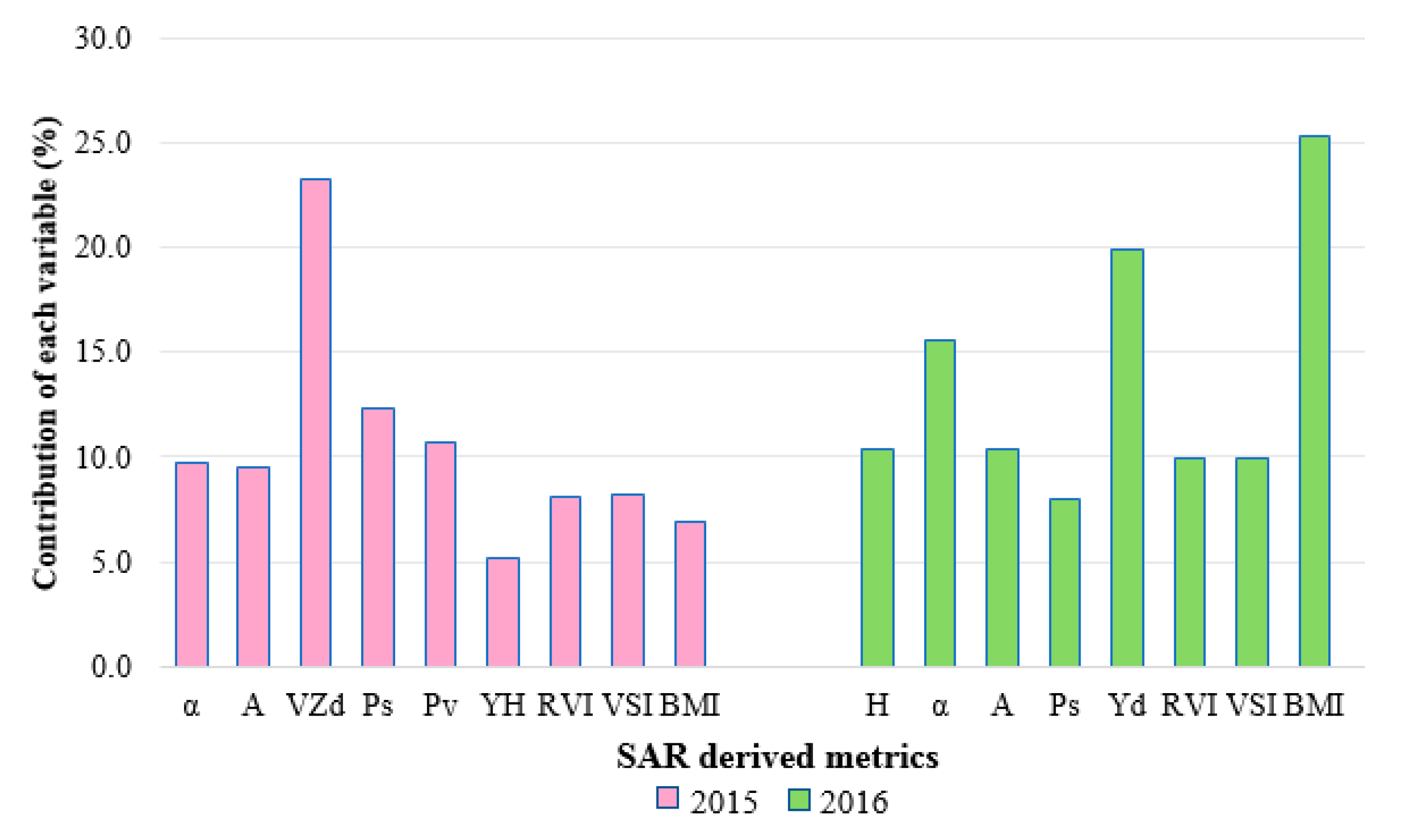
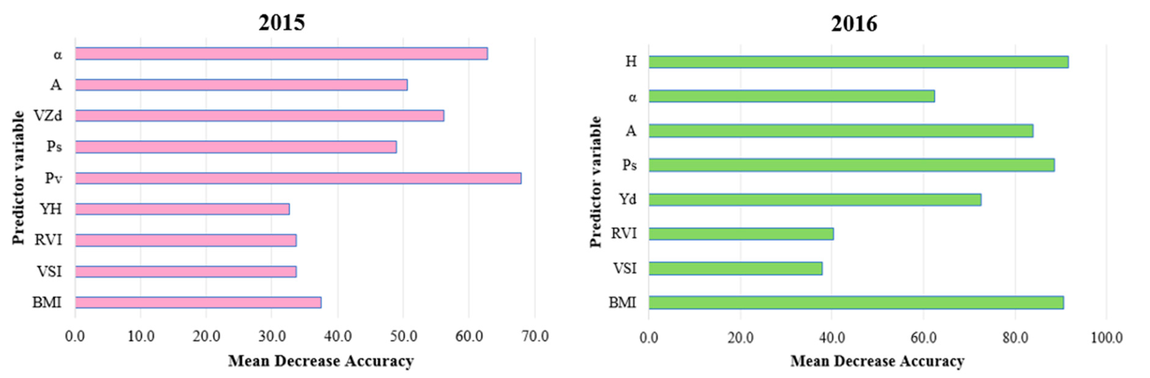
According to the classification results from the optimum subset of attributes for 2015 (α, A, P_v, and VZ_d) and 2016 (H, A, P_s, and BMI) (Table 5), these groups also showed a satisfactory capability to discriminate LULC classes. P_v and H attributes are more sensitive to volumetric scattering and are mainly associated with dense forest classes. Thus, both attributes can be associated with a higher scattering volume of SAR signals in more dense forest structures. Trisasongko [91] used the CP decomposition to monitor disturbances in a dense tropical forest in Papua Tengah Province, Indonesia. This author associated high H values with intact forest classes, indicating a volume scattering mechanism’s dominance. Silva et al. [92] modeled and estimated forest biomass from ALOS/PALSAR-1 polarimetric data in from the TNF and found a significant P_v attribute contribution in primary and secondary forests. According to the results obtained by Kuplich et al. [93], P_v component also presented the highest contribution in the discrimination of LULC classes of the TNF and its surroundings. In relation to classes with dense forest coverage, a greater contribution of BMI index in SAR signal response is expected since this parameter is related to the quantity of AGB. This index tends to be more sensitive in areas of dense forests, which is the case of the TNF.

Concerning A and VZ_d attributes, Tanase et al. [94] found a better correlation with severe burning levels in forests affected by fire in a Mediterranean region for C-band data acquired at steep incidences. Martins et al. [38] and Plank et al. [95] used full polarimetric data from ALOS/PALSAR, obtaining high A values in forested areas severely affected by fire because of an increase of canopy openings and a decrease of AGB.

The P_s attribute is more sensitive to surface scattering mechanism and can be associated with areas with less vegetation coverage or nonforest areas, such as bare soil and water bodies. Qi et al. [96] observed that the dominance of surface scattering extracted from the FD decomposition, which helped distinguishing between forest and barren/sparsely vegetated classes. In the context of the present study, the P_s attribute can be associated mainly with bare soil and croplands, especially at the beginning of the crop growing cycle. The plants are starting to emerge above the surface; and consequently, there is a higher influence of soil surface in the backscattered SAR signals.

In this study, the YH polarimetric decomposition classified by the RF algorithm showed the best results in terms of OA and Kappa index for most of the thematic classes, including forest degradation class, in both years. In this context, Varghese et al. [32] analyzed different polarimetric decompositions to classify forest canopy density, based on the full polarimetric RADARSAT-2 data classified by the SVM algorithm. YH decomposition also showed the best results, followed by VZ, FD, and CP decompositions. Classes with low levels of vegetation coverage, such as cropland and fallows, showed good classification results. In this context, both classes that also were analyzed in our study exhibited similar classification results (Figure 8 and Figure 9). Avtar et al. [89] also used YH, FD, and CP polarimetric decompositions to monitor land cover in a tropical region of Cambodia, based on ALOS/PALSAR-1 full polarimetric data. The authors used the Maximum Likelihood algorithm to classify the decomposition attributes, obtaining the highest value of accuracy, in terms of OA and Kappa index, for the YH decomposition, followed by FD and CP decompositions. Both studies reported above corroborate the results found in our research.

However, some studies presented different classification results. Middinti et al. [97] used ALOS/PALSAR full polarimetric data to classify different forest types from northeastern India. These authors extracted different attributes derived from backscatter coefficients and polarimetric decompositions. The results found for SVM (CP, FD, YH, and VZ decompositions) exhibited nearly similar classification accuracies, with intermediate values. Different to results presented by these authors, the classification results found in our study showed that YH and FD decompositions obtained high values of accuracy. Pôssa et al. [35] also analyzed the different polarimetric decompositions in order to map LULC classes from TNF. CP decomposition showed the best classification results (OA of 77.37% and Kappa index of 0.70), followed by FD and YH decompositions. Mirelva and Nagasawa [98] analyzed FD and YH decompositions, in addition to the backscatter intensities separately, and integrated them into ALOS/PALSAR-1 full polarimetric images for agriculture croplands classification in Indonesia. In their research, the FD and YH decompositions exhibited intermediate overall classification accuracy. Meanwhile, the best classification results were obtained in the integration of backscatter intensities (HH, HV, VH, VV, and HH+HV) and FD decomposition.

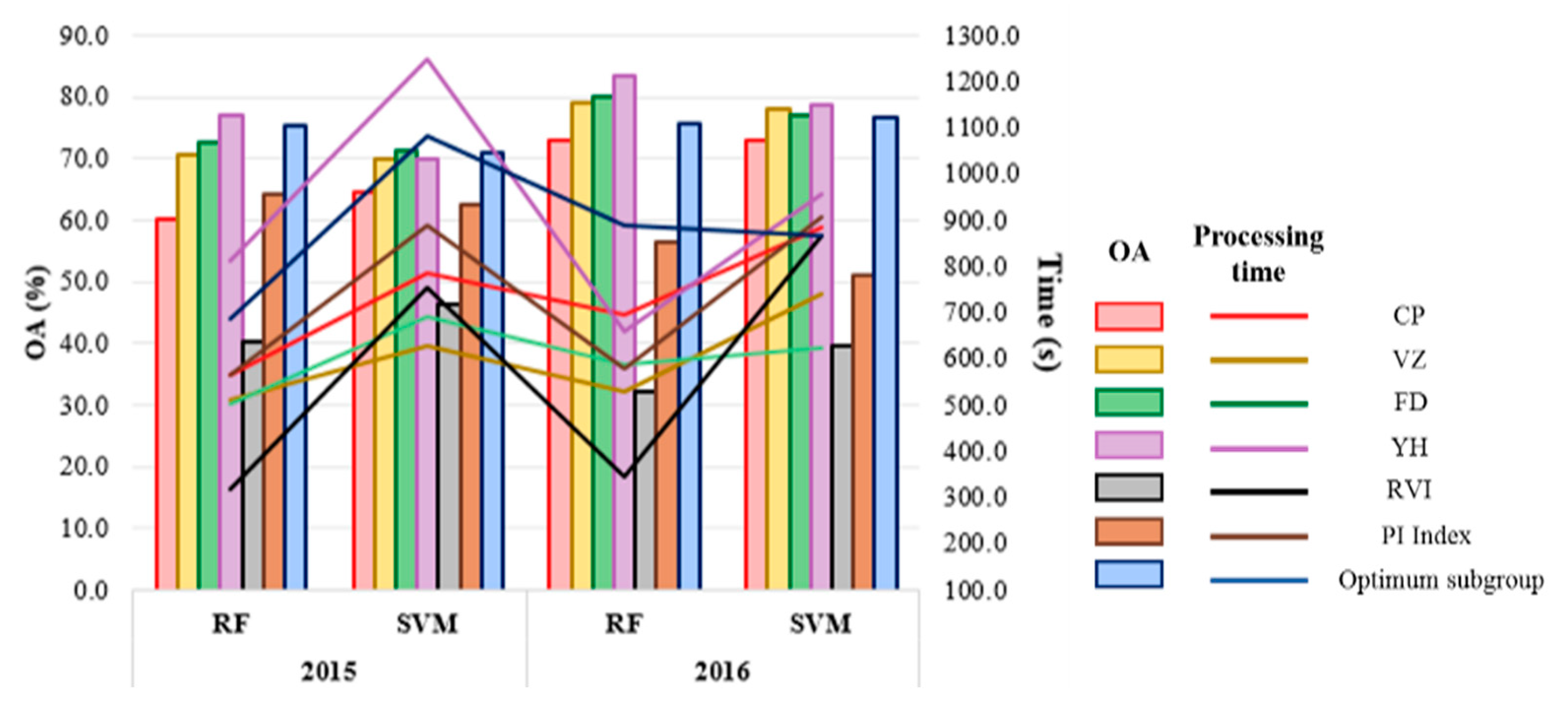
The classification results obtained by VZ, FD, and YH polarimetric decompositions and by the optimum subset demonstrated better classification performances in comparison with the classification based on backscatter coefficients, such as RVI and Pope index (Table 5 and Table 6). A performance investigation of the two advanced machine learning methods (RF and SVM), based on classification accuracy, demonstrated that both algorithms showed sensitivity to discriminate different LULC classes and forest degradation. RF presented the best computational efficiency (Figure 7). The higher processing time in YH and optimal subset classifications for 2015 and 2016 may be related to the larger number of components (4), compared with the other groups (3 and 1).

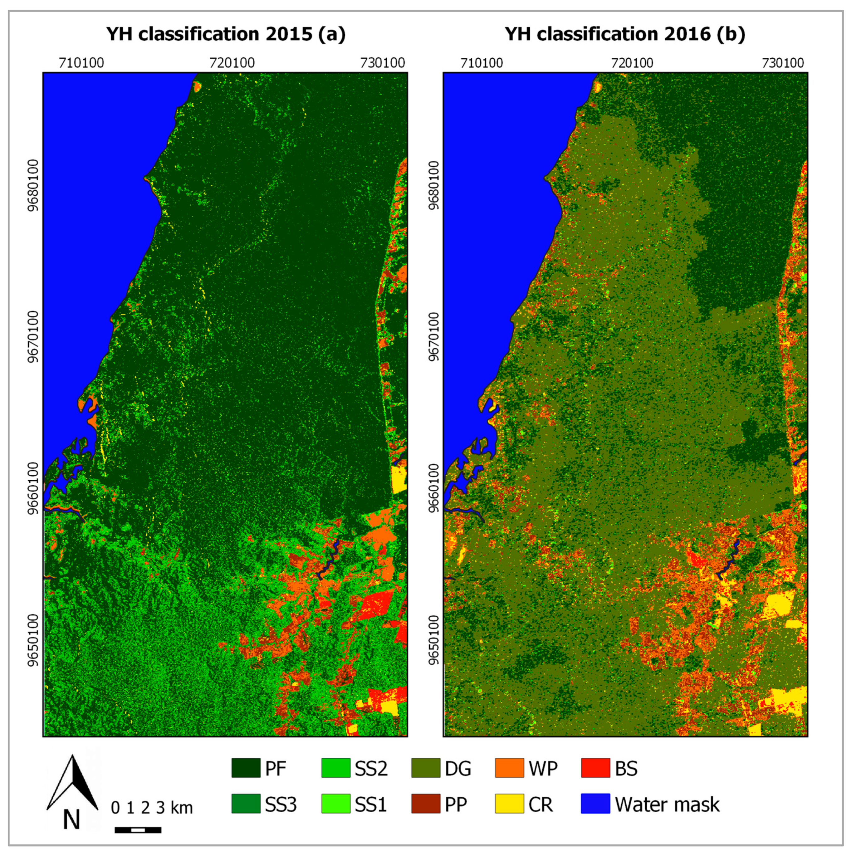
Among the classes with different ecological successions (Figure 12), the most noteworthy class observed from 2015 to 2016 was the DG class. Unusual relative low air humidity, high temperature, and shortage of rainfall events were reported by MODIS products [50,51]. A set of 91 heat points were detected inside the TNF and adjacent areas. In this context, forest degradation, deforestation, and expansion of agricultural and livestock frontiers often cause negative environmental impacts. In order to mitigate these negative impacts, we recommend an effective monitoring and surveillance program in the TNF region.

In this study, only full polarimetric data from ALOS/PALSAR-2 were explored. However, further studies are recommended adding full polarimetric SAR data obtained at different frequencies (currently available from the RADARSAT-2 and the experimental mode TERRASAR-X satellites). Deep learning methods are also recommended to extract more information from targets, thus improving the classification accuracy.

5. Conclusions

The polarimetric attributes extracted from ALOS/PALSAR-2 imagery and classified by RF and SVM algorithms exhibited a good ability to discriminate different types of tropical forests. In terms of OA, Kappa index, and processing time, the RF algorithm, in general, presented the best performance, when compared with that of SVM. YH decomposition, classified by the RF algorithm, presented the best performance concerning LULC and forest degradation classification. The thematic classes with less vegetation coverage were better discriminated than more dense forest structure classes, except for the PF. YH decomposition showed a strong capability of discrimination, with accuracies above 78.0%. However, in terms of processing time, the four components extracted from YH demanded the longest processing times.

The optimum subset of attributes for 2015 (α, A, P_v, and VZ_d) and for 2016 (H, A, P_s, and BMI) and FD and VZ decompositions also showed satisfactory classification results, indicating an adequate capability to discriminate different types of LULC present in rainforests. These polarimetric decompositions involving three attributes showed the shortest processing time performance compared with that of the optimum subgroup. The polarimetric decompositions showed a better performance than the backscatter coefficients represented by RVI and Pope index. During the period 2015–2016, there was a loss of forest classes due to forest degradation caused by fire events. In this context, the classification based on YH decomposition involving the ALOS/PALSAR-2 full polarimetric images demonstrated the capability to discriminate burned areas in rainforests. Furthermore, forest degradation by fire and the conversion of forest into pasture or cropland was also noticed, demanding initiatives to monitor LULC changes in such an important conservation unit. Future research employing deep learning methods, besides a synergistic approach involving other frequency SAR data, is recommended.

Further research for verifying the impact of the time difference between field data collection and SAR data acquisitions on the LULC changes are strongly recommended. Seasonality effects and temporal changes can induce some mislabeled samples in classification models, mainly when collected in land use classes with high temporal and spatial dynamics.

References

1. IBGE. Amazônia Legal. Available online: https://www.ibge.gov.br/geociencias/cartas-e-mapas/mapas-regionais/15819-amazonia-legal.html?=&t=o-que-e (accessed on 9 July 2020).
2. Diniz, C.G.; Souza, A.A.; Santos, D.C.; Dias, M.C.; Luz, N.C.; Moraes, D.R.V.; Maia, J.S.A.; Gomes, A.R.; Narvaes, I.S.; Valeriano, D.M.; et al. DETER-B: The new Amazon near real-time deforestation detection system. IEEE J. Sel. Top. Appl. Earth Obs. Remote Sens. 2015, 8, 3619–3628. [Google Scholar] [CrossRef]
3. Gloor, E. The fate of Amazonia. Nat. Clim. Chang. 2019, 9, 355–356. [Google Scholar] [CrossRef]
4. Andresen, E.; Arroyo-Rodríguez, V.; Escobar, F. Tropical Biodiversity: The Importance of Biotic Interactions for Its Origin, Maintenance, Function, and Conservation. In Ecological Networks in the Tropics; Dáttilo, W., Rico-Gray, V., Eds.; Springer: Cham, Switzerland, 2018; pp. 1–13. [Google Scholar]
5. Alamgir, M.; Campbell, M.J.; Turton, S.M.; Pert, P.L.; Edwards, W.; Laurance, W.F. Degraded tropical rainforests possess valuable carbon storage opportunities in a complex, forested landscape. Sci. Rep. 2016, 6, 1–10. [Google Scholar] [CrossRef]
6. West, T.A.P.; Borner, J.; Fearnside, P.M. Climatic benefits from the 2006–2017 avoided deforestation in Amazonian Brazil. Front. For. Glob. Chang. 2019, 2, 1–11. [Google Scholar] [CrossRef]
7. INPE. Taxas de Desmatamento. Available online: http://terrabrasilis.dpi.inpe.br/app/dashboard/deforestation/biomes/legal_amazon/rates (accessed on 5 May 2019).
8. INPE. Estimates for the Amazon: Deforestation-Driven Gross Emissions (Old Growth Forests). Available online: http://inpe-em.ccst.inpe.br/en/estimates-for-the-amazon/ (accessed on 7 October 2020).
9. Gibbs, H.K.; Ruesch, A.S.; Achard, F.; Clayton, M.K.; Holmgren, P.; Ramankutty, N.; Foley, J.A. Tropical forests were the primary sources of new agricultural land in the 1980s and 1990s. Proc. Natl. Acad. Sci. USA 2010, 107, 16732–16737. [Google Scholar] [CrossRef] [Green Version]
10. Gomez, M.D.V.; Beuchle, R.; Shimabukuro, Y.; Grecchi, R.; Simonetti, D.; Eva, H.D.; Achard, F. A long-term perspective on deforestation rates in the Brazilian Amazon. Int. Arch. Photogramm. Remote Sens. Spat. Inf. Sci. ISPRS Arch. 2015, 40, 539–544. [Google Scholar] [CrossRef] [Green Version]
11. Barlow, J.; Berenguer, E.; Carmenta, R.; França, F. Clarifying Amazonia’s burning crisis. Glob. Chang. Biol. 2019, 2019, 1–3. [Google Scholar] [CrossRef] [Green Version]
12. Escobar, H. Amazon fires clearly linked to deforestation, scientists say. Science 2019, 365, 853. [Google Scholar] [CrossRef]
13. INPE. Monitoramento Dos Focos Ativos Por Bioma. Available online: http://queimadas.dgi.inpe.br/queimadas/portal-static/estatisticas_estados/ (accessed on 24 July 2020).
14. Bebber, D.P. The Brazilian Amazon protected area network was largely unaffected by recent satellite-detectable fires. bioRxiv 2019, 1–7. [Google Scholar] [CrossRef] [Green Version]
15. Davidson, E.A.; Araújo, A.C.; Artaxo, P.; Balch, J.K.; Brown, I.F.; Bustamante, M.C.; Coe, M.; Defries, R.S.; Keller, M.; Longo, M.; et al. The Amazon basin in transition. Nature 2012, 481, 321–328. [Google Scholar] [CrossRef]
16. Lewis, S.L.; Edwards, D.P.; Galbraith, D. Increasing human dominance of tropical forests. Science 2015, 349, 827–832. [Google Scholar] [CrossRef] [PubMed]
17. Laurance, W.F.; Vasconcelos, H.L.; Lovejoy, T.E. Forest loss and fragmentation in the Amazon: Implications for wildlife conservation. Oryx 2000, 34, 39–45. [Google Scholar] [CrossRef]
18. Barlow, J.; Lennox, G.D.; Ferreira, J.; Berenguer, E.; Lees, A.C.; Nally, R.M.; Thomson, J.R.; Ferraz, S.F.D.B.; Louzada, J.; Oliveira, V.H.F.; et al. Anthropogenic disturbance in tropical forests can double biodiversity loss from deforestation. Nature 2016, 535, 144–147. [Google Scholar] [CrossRef] [PubMed] [Green Version]
19. Diele-Viegas, L.M.; Rocha, C.F.D. Why releasing mining on Amazonian indigenous lands and the advance of agrobusiness is extremely harmful for the mitigation of world’s climate change? Comment on Pereira et al. (Environmental Science & Policy 100 (2019) 8–12). Environ. Sci. Policy 2020, 103, 30–31. [Google Scholar]
20. Ricketts, T.H.; Soares-Filho, B.; Fonseca, G.A.B.; Nepstad, D.; Pfaf, A.; Petsonk, A.; Anderson, A.; Boucher, D.; Cattaneo, A.; Conte, M.; et al. Indigenous lands, protected areas, and slowing climate change. PLoS Biol. 2010, 8, e1000331. [Google Scholar] [CrossRef]
21. Souza, A.; Monteiro, A.M.V.; Rennó, C.D.; Almeida, C.A.; Valeriano, D.M.; Morelli, F.; Vinhas, L.; Maurano, L.E.P.; Adami, M.; Escada, M.I.S.; et al. Metodologia Utilizada nos Projetos PRODES e DETER; INPE: São José dos Campos, Brazil, 2019. [Google Scholar]
22. INPE. Monitoramento dos focos Ativos por Estado. Available online: http://queimadas.dgi.inpe.br/queimadas/portal-static/estatisticas_estados/ (accessed on 24 July 2020).
23. TCU. Relatório de Auditoria Operacional, Unidade de Conservação Floresta Nacional do Tapajós. Available online: http://www.tcu.gov.br/Consultas/Juris/Docs/judoc%5CAcord%5C20080516%5C004-088-2004-0-AN-Agrupados.doc (accessed on 17 November 2019).
24. Andrade, D.F.C.D.; Gama, J.R.V.; Ruschel, A.R.; Melo, L.O.; Avila, A.L.D.; Carvalho, J.O.P.D. Post-fire recovery of a dense ombrophylous forest in Amazon. An. Acad. Bras. Cienc. 2019, 91, 1–11. [Google Scholar] [CrossRef] [Green Version]
25. Brazil. Law n 12.678, from 25 June 2012. Available online: http://www.planalto.gov.br/ccivil_03/_Ato2011-2014/2012/Lei/L12678.htm (accessed on 18 June 2019).
26. Metzger, J.P.; Bustamante, M.M.C.; Ferreira, J.; Fernandes, G.W.; Librán-Embid, F.; Pillar, V.D.; Prist, P.R.; Rodrigues, R.R.; Vieira, I.C.G.; Overbeck, G.E. Why Brazil needs its legal reserves. Perspect. Ecol. Conserv. 2019, 17, 91–103. [Google Scholar] [CrossRef]
27. Fichera, C.R.; Modica, G.; Pollino, M. Land cover classification and change-detection analysis using multi-temporal remote sensed imagery and landscape metrics. Eur. J. Remote Sens. 2012, 45, 1–18. [Google Scholar] [CrossRef]
28. Guerra, J.B.; Mura, J.C.; Freitas, C.C. Discriminação de incrementos de desflorestamento na Amazônia com dados SAR R99B em banda L. Acta Amaz. 2010, 40, 557–566. [Google Scholar] [CrossRef] [Green Version]
29. Negri, R.G.; Dutra, L.V.; Freitas, C.C.; Dengsheng, L. Exploring the capability of ALOS PALSAR L-band fully polarimetric data for land cover classification in tropical environments. IEEE J. Sel. Top. Appl. Earth Obs. Remote Sens. 2016, 9, 5369–5384. [Google Scholar] [CrossRef]
30. Cazcarra-Bes, V.; Tello-Alonso, M.; Fischer, R.; Heym, M.; Papathanassiou, K. Monitoring of forest structure dynamics by means of L-band SAR tomography. Remote Sens. 2017, 9, 1229. [Google Scholar] [CrossRef] [Green Version]
31. Li, G.; Lu, D.; Moran, E.; Dutra, L.; Batistella, M. A comparative analysis of ALOS PALSAR L-band and RADARSAT-2 C-band data for land-cover classification in a tropical moist region. ISPRS J. Photogramm. Remote Sens. 2012, 70, 26–38. [Google Scholar] [CrossRef] [Green Version]
32. Varghese, A.O.; Suryavanshi, A.; Joshi, A.K. Analysis of different polarimetric target decomposition methods in forest density classification using C-band SAR data. Int. J. Remote Sens. 2016, 37, 694–709. [Google Scholar] [CrossRef]
33. Chen, W.; Jiang, H.; Moriya, K.; Sakai, T.; Cao, C. Monitoring of post-fire forest regeneration under different restoration treatments based on ALOS/PALSAR data. New For. 2018, 49, 105–121. [Google Scholar] [CrossRef]
34. Urbazaev, M.; Cremer, F.; Migliavacca, M.; Reichstein, M.; Schmullius, C.; Thiel, C. Potential of multi-temporal ALOS-2 PALSAR-2 ScanSAR data for vegetation height estimation in tropical forests of Mexico. Remote Sens. 2018, 10, 1277. [Google Scholar] [CrossRef] [Green Version]
35. Pôssa, E.M.; Gama, F.F.; Santos, J.R.; Mura, J.C.; Bispo, P.C. Análise de uso da terra e cobertura florestal na Amazônia central, a partir de dado polarimétrico PALSAR/ALOS-1 e coerência interferométrica TanDEM-X. Rev. Bras. Geogr. Física 2018, 11, 2094–2108. [Google Scholar] [CrossRef] [Green Version]
36. Pereira, L.O.; Freitas, C.C.; Sant’Anna, S.J.S.; Reis, M.S. ALOS/PALSAR data evaluation for land use and land cover mapping in the Amazon region. IEEE J. Sel. Top. Appl. Earth Obs. Remote Sens. 2016, 9, 5413–5423. [Google Scholar] [CrossRef]
37. Mermoz, S.; Le Toan, T. Forest disturbances and regrowth assessment using ALOS PALSAR data from 2007 to 2010 in Vietnam, Cambodia and Lao PDR. Remote Sens. 2016, 8, 217. [Google Scholar] [CrossRef] [Green Version]
38. Martins, F.S.R.V.; Santos, J.R.; Galvão, L.S.; Xaud, H.A.M. Sensitivity of ALOS/PALSAR imagery to forest degradation by fire in northern Amazon. Int. J. Appl. Earth Obs. Geoinf. 2016, 49, 163–174. [Google Scholar] [CrossRef]
39. Pavanelli, J.A.P.; Santos, J.R.; Galvão, L.S.; Xaud, M.R.; Xaud, H.A.M. Palsar-2/ALOS-2 and Oli/Landsat-8 data integration for land use and land cover mapping in northern Brazilian Amazon. Bol. Ciênc. Geod. 2018, 24, 250–269. [Google Scholar] [CrossRef]
40. De Alban, J.D.T.; Connette, G.M.; Oswald, P.; Webb, E.L. Combined Landsat and L-band SAR data improves land cover classification and change detection in dynamic tropical landscapes. Remote Sens. 2018, 10, 306. [Google Scholar] [CrossRef] [Green Version]
41. Hagensieker, R.; Waske, B. Evaluation of multi-frequency SAR images for tropical land cover mapping. Remote Sens. 2018, 10, 257. [Google Scholar] [CrossRef] [Green Version]
42. Copping, P.R.; Bauer, M.E. Digital change detection in forest ecossystems with remote sensing imagery. Remote Sens. 1996, 13, 207–234. [Google Scholar]
43. Lu, D.; Mausel, P.; Brondízio, E.; Moran, E. Change detection techniques. Int. J. Remote Sens. 2004, 25, 2365–2407. [Google Scholar] [CrossRef]
44. Cakir, H.I.; Khorram, S.; Nelson, S.A.C. Correspondence analysis for detecting land cover change. Remote Sens. Environ. 2006, 102, 306–317. [Google Scholar] [CrossRef]
45. Desclée, B.; Bogaert, P.; Defourny, P. Forest change detection by statistical object-based method. Remote Sens. Environ. 2006, 102, 1–11. [Google Scholar] [CrossRef]
46. Grant, R.F.; Hutyra, L.R.; Oliveira, R.C.; Munger, J.W.; Saleska, S.R.; Wofsy, C. Modeling the carbon balance of Amazonian rainforests: Resolving ecological controls on net ecosystem productivity. Ecol. Monogr. 2009, 79, 445–463. [Google Scholar] [CrossRef]
47. Bispo, P.C.; Santos, J.R.; Valeriano, M.M.; Touzi, R.; Seifert, F.M. Integration of polarimetric PALSAR attributes and local geomorphometric variables derived from SRTM for forest biomass modeling in central Amazonia. Can. J. Remote Sens. 2014, 40, 26–42. [Google Scholar] [CrossRef]
48. Bispo, P.C.; Pardini, M.; Papathanassiou, K.P.; Kugler, F.; Balzter, H.; Rains, D.; Santos, J.R.; Rizaev, I.G.; Tansey, K.; Santos, M.N.; et al. Mapping forest successional stages in the Brazilian Amazon using forest heights derived from TanDEM-X SAR interferometry. Remote Sens. Environ. 2019, 232, 111194. [Google Scholar] [CrossRef]
49. Ricklefs, R.; Relyea, R. Ecology: The Economy of Nature, 7th ed.; W.H. Freeman: New York, NY, USA, 2013. [Google Scholar]
50. Yang, Y.; Saatchi, S.S.; Xu, L.; Yu, Y.; Choi, S.; Phillips, N.; Kennedy, R.; Keller, M.; Knyazikhin, Y.; Myneni, R.B. Post-drought decline of the Amazon carbon sink. Nat. Commun. 2018, 9, 1–9. [Google Scholar] [CrossRef] [PubMed]
51. Wiederkehr, N.C.; Gama, F.F.; Mura, J.C.; Santos, J.R.; Bispo, P.C.; Sano, E.E. Analysis of the target decomposition technique attributes and polarimetric ratios to discriminate land use and land cover classes of the Tapajós region. Bol. Ciênc. Geod. 2019, 25, 1–16. [Google Scholar] [CrossRef]
52. Silva, R.D.; Galvão, L.S.; Santos, J.R.; Silva, C.V.J.; Moura, Y.M. Spectral/textural attributes from ALI/EO-1 for mapping primary and secondary tropical forests and studying the relationships with biophysical parameters. GISci. Remote Sens. 2014, 51, 677–694. [Google Scholar] [CrossRef]
53. Silva, C.V.J.; Santos, J.R.; Galvão, L.S.; Silva, R.D.; Moura, Y.M. Floristic and structure of an Amazonian primary forest and a chronosequence of secondary succession. Acta Amaz. 2016, 46, 133–150. [Google Scholar] [CrossRef] [Green Version]
54. Vieira, I.C.G.; Almeida, A.S.; Davidson, E.A.; Stone, T.A.; Carvalho, C.J.R.; Guerrero, J.B. Classifying successional forests using Landsat spectral properties and ecological characteristics in eastern Amazônia. Remote Sens. Environ. 2003, 87, 470–481. [Google Scholar] [CrossRef]
55. Uhl, C.; Buschbacher, R.; Serrao, E.A.S. Abandoned pastures in eastern Amazonia. I. Patterns of plant succession. J. Ecol. 1988, 76, 663–681. [Google Scholar] [CrossRef]
56. Lee, J.; Grunes, M.R.; Grandi, G. Polarimetric SAR speckle filtering and its implication for classification. IEEE Trans. Geosci. Remote Sens. 1999, 37, 2363–2373. [Google Scholar]
57. Cloude, S.R.; Pottier, E. A review of target decomposition theorems in radar polarimetry. IEEE Trans. Geosci. Remote Sens. 1996, 34, 498–518. [Google Scholar] [CrossRef]
58. Van Zyl, J.J. Application of Cloude’s target decomposition theorem to polarimetric imaging radar data. Radar Polarim. SPIE 1992, 184–191. [Google Scholar]
59. Freeman, A.; Durden, S.L. A three-component scattering model for polarimetric SAR data. IEEE Trans. Geosci. Remote Sens. 1998, 36, 963–973. [Google Scholar] [CrossRef] [Green Version]
60. Yamaguchi, Y.; Moriyama, T.; Ishido, M.; Yamada, H. Four-component scattering model for polarimetric SAR image decomposition. IEEE Trans. Geosci. Remote Sens. 2005, 43, 1699–1706. [Google Scholar] [CrossRef]
61. Sun, S.; Liu, R.; Wen, W. Unsupervised classification method for polarimetric synthetic aperture radar imagery based on Yamaguchi four-component decomposition model. J. Electr. Comput. Eng. 2015, 2015, 1–7. [Google Scholar] [CrossRef] [Green Version]
62. Kim, Y.; van Zyl, J.J. A time-series approach to estimate soil moisture using polarimetric radar data. IEEE Trans. Geosci. Remote Sens. 2009, 47, 2519–2527. [Google Scholar]
63. Pope, K.O.; Rey-Benayas, J.M.; Paris, J.F. Radar remote sensing of forest and wetland ecosystems in the Central American tropics. Remote Sens. Environ. 1994, 48, 205–219. [Google Scholar] [CrossRef]
64. Goumehei, E.; Tolpekin, V.; Stein, A.; Yan, W. Surface water body detection in polarimetric SAR data using contextual complex Wishart classification. Water Resour. Res. 2019, 55, 7047–7059. [Google Scholar] [CrossRef] [Green Version]
65. ANA. Rios Principais. Available online: https://metadados.ana.gov.br/geonetwork/srv/pt/main.home (accessed on 17 November 2019).
66. Exelis Visual Information Solutions-ENVI, v. 5.0; EXELIS: Boulder, Colorado, 2014.
67. Mendes, F.S.; Baron, D.; Gerold, G.; Liesenberg, V.; Erasmi, S. Optical and SAR remote sensing synergism for mapping vegetation types in the endangered Cerrado/Amazon ecotone of Nova Mutum-Mato Grosso. Remote Sens. 2019, 11, 1161. [Google Scholar] [CrossRef] [Green Version]
68. Jolliffe, I.T. Principal Component Analysis; Springer: New York, NY, USA, 2002. [Google Scholar]
69. Li, Q.; Gong, L.; Zhang, J. A correlation change detection method integrating PCA and multi-texture features of SAR image for building damage detection. Eur. J. Remote Sens. 2019, 52, 435–447. [Google Scholar] [CrossRef] [Green Version]
70. Mackiewicz, A.; Ratajczak, W. Principal Components Analysis (PCA). Comput. Geosci. 1993, 19, 303–342. [Google Scholar] [CrossRef]
71. R Core Team. R: A language and environment for statistical computing. Viena, R Foundation for Statistical Computing. 2020. Available online: https://www.R-project.org/ (accessed on 10 September 2019).
72. Camargo, F.F.; Sano, E.E.; Almeida, C.M.; Mura, J.C.; Almeida, T. A comparative assessment of machine-learning techniques for land use and land cover classification of the Brazilian tropical savanna using ALOS-2/PALSAR-2 polarimetric images. Remote Sens. 2019, 45, 1600. [Google Scholar] [CrossRef] [Green Version]
73. Furtado, L.F.A.; Silva, T.S.F.; Novo, E.M.L.M. Dual-season and full-polarimetric C band SAR assessment for vegetation mapping in the Amazon varzea wetlands. Remote Sens. Environ. 2016, 174, 212–222. [Google Scholar] [CrossRef] [Green Version]
74. Du, P.; Samat, A.; Waske, B.; Liu, S.; Li, Z. Random Forest and Rotation Forest for fully polarized SAR image classification using polarimetric and spatial features. ISPRS J. Photogramm. Remote Sens. 2015, 105, 38–53. [Google Scholar] [CrossRef]
75. Diniz, J.M.F.S.; Gama, F.F.; Adami, M. Evaluation of polarimetry and interferometry of Sentinel-1A SAR data for land use and land cover of the Brazilian Amazon region. Geocarto Int. 2020, 6049, 1–17. [Google Scholar] [CrossRef]
76. Shiraishi, T.; Motohka, T.; Thapa, R.B.; Watanabe, M.; Shimada, M. Comparative assessment of supervised classifiers for land use-land cover classification in a tropical region using time-series PALSAR mosaic data. IEEE J. Sel. Top. Appl. Earth Obs. Remote Sens. 2014, 7, 1186–1199. [Google Scholar] [CrossRef]
77. Numbisi, F.N.; van Coillie, F.; Wulf, R. Multi-date Sentinel-1 SAR image textures discriminate perennial agroforests in a tropical forest-savannah transition landscape. Int. Arch. Photogramm. Remote Sens. Spat. Inf. Sci. 2018, 42, 339–346. [Google Scholar] [CrossRef] [Green Version]
78. Breiman, L. Random Forests. Mach. Learn. 2001, 45, 5–32. [Google Scholar] [CrossRef] [Green Version]
79. Eisavi, V.; Homayouni, S.; Yazdi, A.M.; Alimohammadi, A. Land cover mapping based on random forest classification of multitemporal spectral and thermal images. Environ. Monit. Assess. 2015, 187, 1–14. [Google Scholar] [CrossRef] [PubMed]
80. Wang, Y.; Chen, W.; Huang, K.; Gu, Q. Classification of neonatal amplitude-integrated EEG using random forest model with combined feature. In Proceedings of the IEEE International Conference on Bioinformatics and Biomedicine (BIBM), Shanghai, China, 18–21 December 2013; pp. 285–290. [Google Scholar]
81. Cutler, D.R.; Edwards, T.C.; Beard, K.H.; Cutler, A.; Kyle, T.; Gibson, J.; Lawler, J.J.; Beard, H.; Hess, T. Random Forests for classification in ecology. Ecology 2007, 88, 2783–2792. [Google Scholar] [CrossRef] [PubMed]
82. Boardman, M.; Trappenberg, T. A heuristic for free parameter optimization with Support Vector Machines. In Proceedings of the IEEE International Joint Coference on Neural Network, Vancouver, BC, Canada, 16–21 July 2006; pp. 610–617. [Google Scholar]
83. Vapnik, V.N. Statistical Learning Theory; Haykin, S., Ed.; Wiley: New York, NY, USA, 1998; Volume 3. [Google Scholar]
84. Cortes, C.; Vapnik, V. Support-Vector Networks. Machine Learn. 1995, 20, 273–297. [Google Scholar] [CrossRef]
85. Abe, S. Support Vector Machines for Pattern Classification, 2nd ed.; Springer: London, UK, 2010. [Google Scholar]
86. Vapnik, V.N. The Nature of Statistical Learning Theory; Springer: New York, NY, USA, 1995. [Google Scholar]
87. Meyer, D. Support Vector Machines. The Interface to libsvm in package. Porting R Darwin/X11 Mac OS X 2001, 1, 23. [Google Scholar]
88. Henderson, F.M.; Lewis, A.J. Manual of Remote Sensing: Principles and Applications of Imaging Radar, 3rd ed.; John Wiley Sons: New York, NY, USA, 1998; 866p. [Google Scholar]
89. Avtar, R.; Takeuchi, W.; Sawada, H. Full polarimetric PALSAR-based land cover monitoring in Cambodia for implementation of REDD policies. Int. J. Digit. Earth 2013, 6, 255–275. [Google Scholar] [CrossRef]
90. Ullmann, T.; Banks, S.N.; Schmitt, A.; Jagdhuber, T. Scattering characteristics of X-, C- and L-band PolSAR data examined for the tundra environment of the Tuktoyaktuk Peninsula, Canada. Appl. Sci. 2017, 7, 595. [Google Scholar] [CrossRef] [Green Version]
91. Trisasongko, B.H. The use of polarimetric SAR data for forest disturbance monitoring. Sens. Imaging 2010, 11, 1–13. [Google Scholar] [CrossRef]
92. Narvaes, I.S.; Santos, J.R.; Silva, A.Q. Analysis of structural parameters of forest typologies using L-band SAR data. Bol. Ciênc. Geod. 2010, 16, 475–489. [Google Scholar] [CrossRef] [Green Version]
93. Kuplich, T.M.; Shimabukuro, Y.E.; Servello, E.; Sano, E. Polarimetric signatures and classification of tropical land covers. In Proceedings of the International Geoscience and Remote Sensing Symposium (IGARSS 2009), Cape Town, South Africa, 12–17 July 2009; University of Cape Town: Cape Town, South Africa, 2009; pp. 118–121. [Google Scholar]
94. Tanase, M.A.; Santoro, M.; Aponte, C.; Riva, J. Polarimetric properties of burned forest areas at C- and L-band. IEEE J. Sel. Top. Appl. Earth Obs. Remote Sens. 2014, 7, 267–276. [Google Scholar] [CrossRef]
95. Plank, S.; Karg, S.; Martinis, S. Full-polarimetric burn scar mapping—The differences of active fire and post-fire situations. Int. J. Remote Sens. 2018, 1–16. [Google Scholar] [CrossRef]
96. Qi, Z.; Yeh, A.G.O.; Li, X.; Lin, Z. A novel algorithm for land use and land cover classification using RADARSAT-2 polarimetric SAR data. Remote Sens. Environ. 2012, 118, 21–39. [Google Scholar] [CrossRef]
97. Middinti, S.; Jha, C.S.; Reddy, T.B. Forest type classification with combination of advanced polarimetric decompositions and textures of L-band synthetic aperture radar data. J. Appl. Remote Sens. 2017, 11, 016035. [Google Scholar] [CrossRef]
98. Mirelva, P.R.; Nagasawa, R. Application of ALOS PALSAR data for agriculture croplands classification in central Java, Indonesia. J. Jpn. Agric. Syst. Soc. 2017, 33, 27–36. [Google Scholar]
99. Van Zyl, J.J.; Arii, M.; Kim, Y. Model-based decomposition of polarimetric SAR covariance matrices constrained for nonnegative eigenvalues. IEEE Trans. Geosci. Remote Sens. 2011, 49, 3452–3459. [Google Scholar] [CrossRef]
Figure 1. Location of the study area in the Pará State (a) and in the Tapajós National Forest (b). The image corresponds to the RGB color composite of HH/HV, VV/VH, and HH/VV ratios of ALOS/PALSAR-2 images mosaic (c) (overpasses in 28 December 2014, 19 April 2015, and 3 May 2015).
Remotesensing 12 03512 g001
Figure 2. Flowchart of the methodology used to discriminate the land use, land cover, and forest degradation in Tapajós National Forest region, Brazil.
Remotesensing 12 03512 g002
Figure 3. Mosaic of three ALOS/PALSAR-2 images covering the study area. The images were obtained on 1 May 2016 (a,c) and on 17 April 2016 (b). The mosaic corresponds to the RGB color composite of HH, HV, and VV polarizations.
Remotesensing 12 03512 g003
Figure 4. Distribution of the ground truths over the nine land use and land cover (LULC) classes found in the study area and represented in the ALOS/PALSAR-2 images from 2015 (a) and 2016 (b). For LULC class identification, see Table 1.
Remotesensing 12 03512 g004
Figure 5. Contribution of each variable derived from PC1 and PC2. Details of the SAR derived metrics are presented in Table 3.
Remotesensing 12 03512 g005
Figure 6. Random Forest’s predictor variables importance measures: mean decrease accuracy for LULC classes for 2015 and 2016. Details of the SAR derived attributes are presented in Table 3.
Remotesensing 12 03512 g006
Figure 7. Performance of the RF and SVM classifiers in relation to the OA and processing time for 2015 and 2016. CP: Cloude–Pottier decomposition; VZ: van Zyl decomposition; FD: Freeman–Durden decomposition; YH: Yamaguchi decomposition; RVI: Radar Vegetation Index; and PI: Pope Index.
Remotesensing 12 03512 g007
Figure 8. Producer’s accuracy, user’s accuracy, and F1-scores of Yamaguchi classification for 2015, based on the RF algorithm. For LULC class identification, see Table 1.
Remotesensing 12 03512 g008
Figure 9. Producer’s accuracy and user’s accuracy of Yamaguchi classification for 2016, based on RF algorithm. For LULC class identification, see Table 1.
Remotesensing 12 03512 g009
Figure 10. Land use, land cover, and forest degradation classification maps of the study area from 2015 (a) and 2016 (b), based on Yamaguchi (YH) decomposition. For LULC class identification, see Table 1.
Remotesensing 12 03512 g010
Figure 11. Location of the study area in the Tapajós National Forest. The image corresponds to the RGB color composite of HH/HV, VV/VH, and HH/VV ratios of ALOS/PALSAR-2 images mosaic (a). Black rectangle represents the land use, land cover, and forest degradation classification subsets of the study area from 2015 (b) and 2016 (c), based on Yamaguchi (YH) decomposition. For LULC class identification, see Table 1.
Remotesensing 12 03512 g011
Figure 12. Location of the study area in the Tapajós National Forest. The images correspond to RGB color composite of HH/HV, VV/VH, and HH/VV ratios of ALOS/PALSAR-2 images mosaic (a). Black rectangles represent land cover and forest degradation by fire (subsets 1, 2, and 3) of the study area: the classification based on Yamaguchi (YH) attributes from 2015, derived from the ALOS/PALSAR-2 polarimetric images (b); its corresponding area imaged by Landsat-8/OLI satellite obtained on August 14, 2015 and shown by the R6G5B4 composition, corresponding to the period before fire events (c); the YH classification from 2016, derived from ALOS/PALSAR-2 (d); and its corresponding area imaged from Landsat-8/OLI satellite obtained June 29, 2016 and shown by the R6G5B4 composition, corresponding to the period after the fire (e). For LULC class identification, see Table 1.
Remotesensing 12 03512 g012