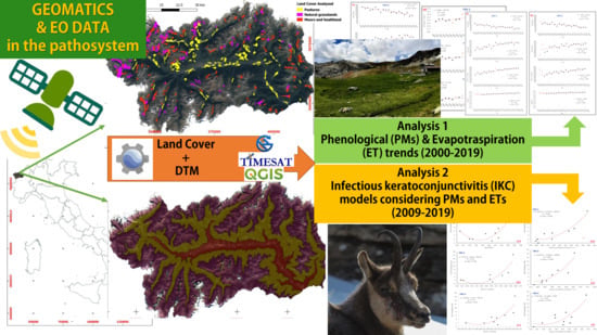
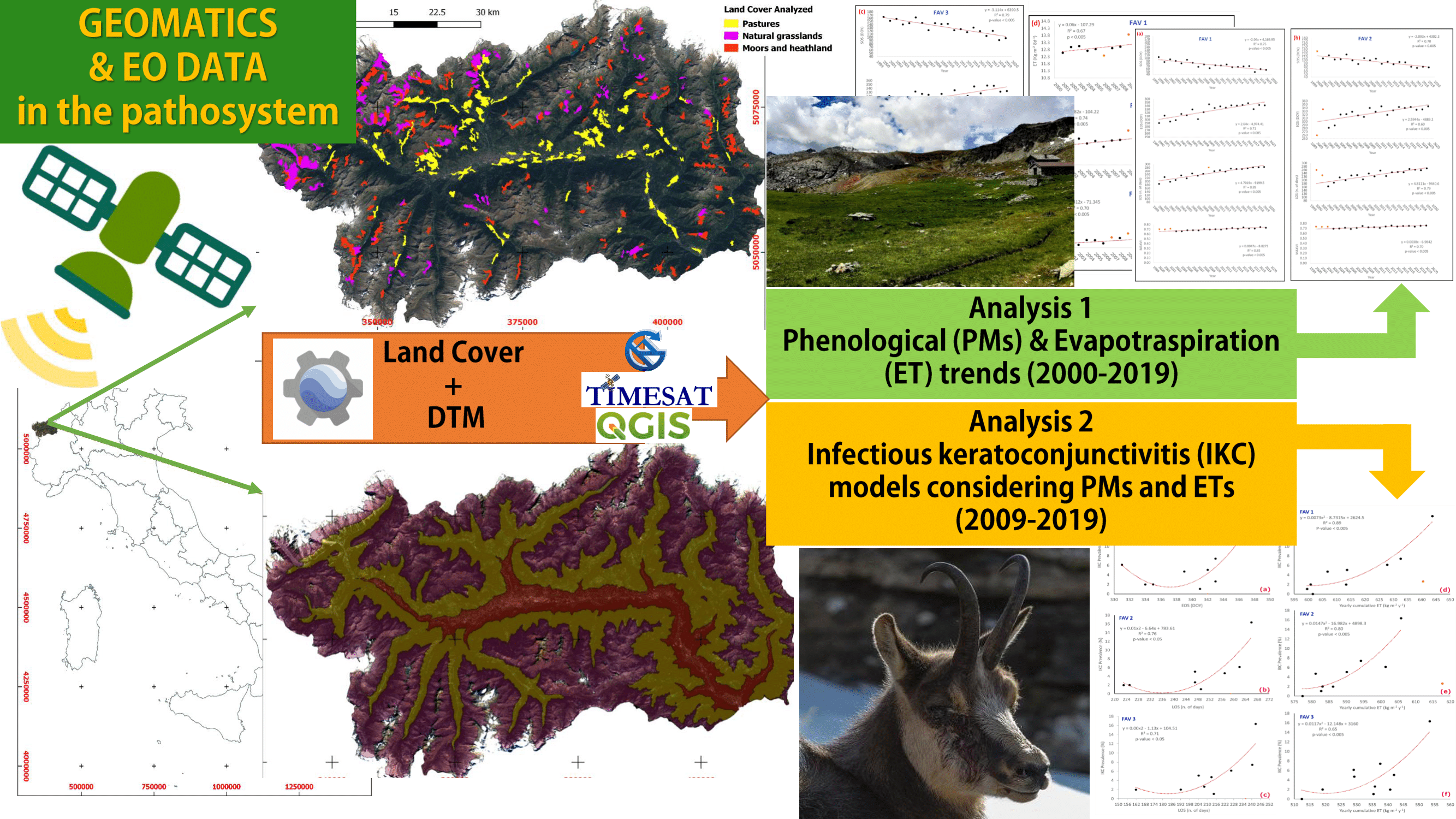
Geomatics and EO Data to Support Wildlife Diseases Assessment at Landscape Level: A Pilot Experience to Map Infectious Keratoconjunctivitis in Chamois and Phenological Trends in Aosta Valley (NW Italy)

 ,
,  and
and 
Abstract
:
1. Introduction
2. Materials and Methods
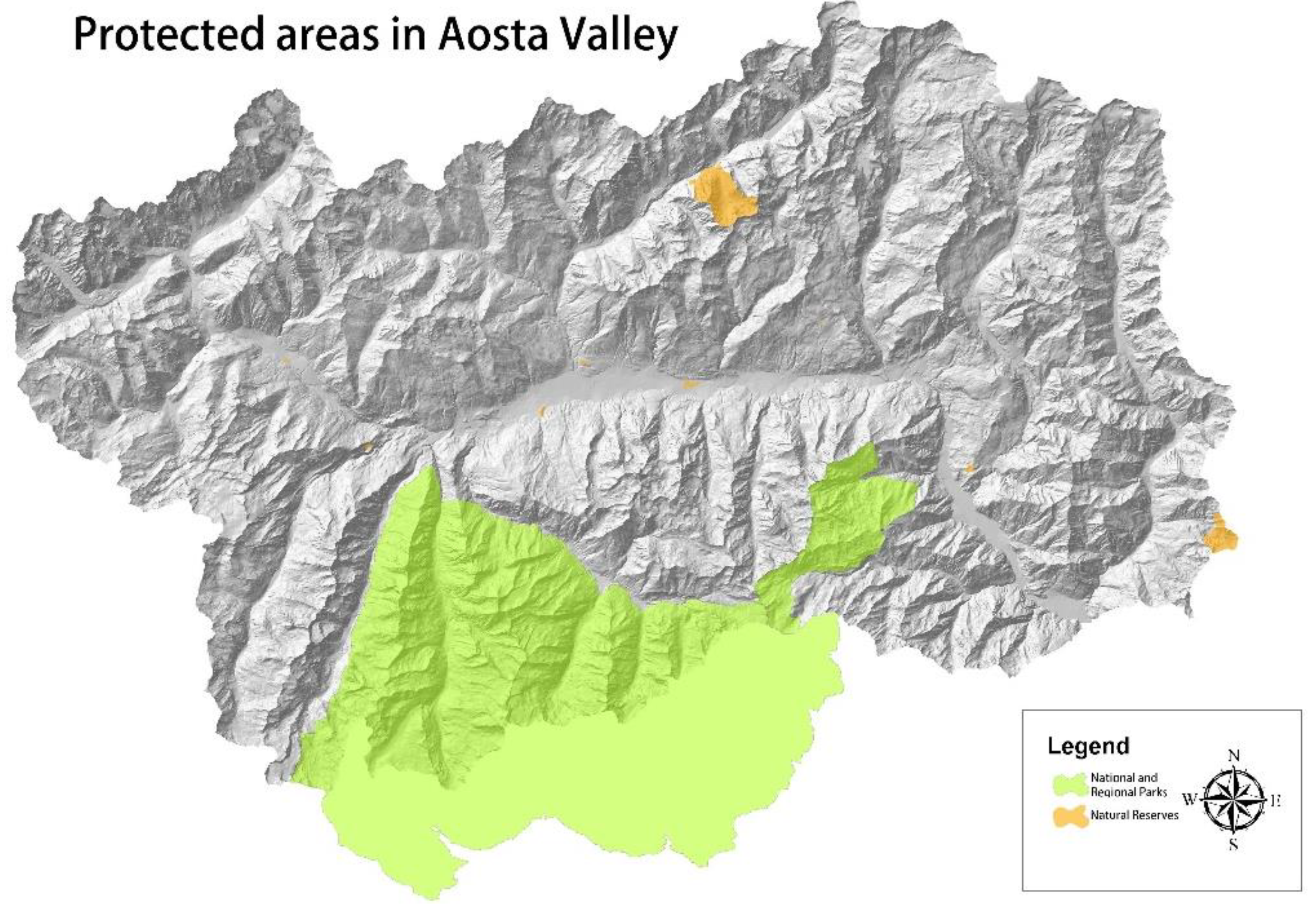
2.1. Study Area
2.2. Veterinary Ground Samples
2.3. EO and Geographical Digital Data
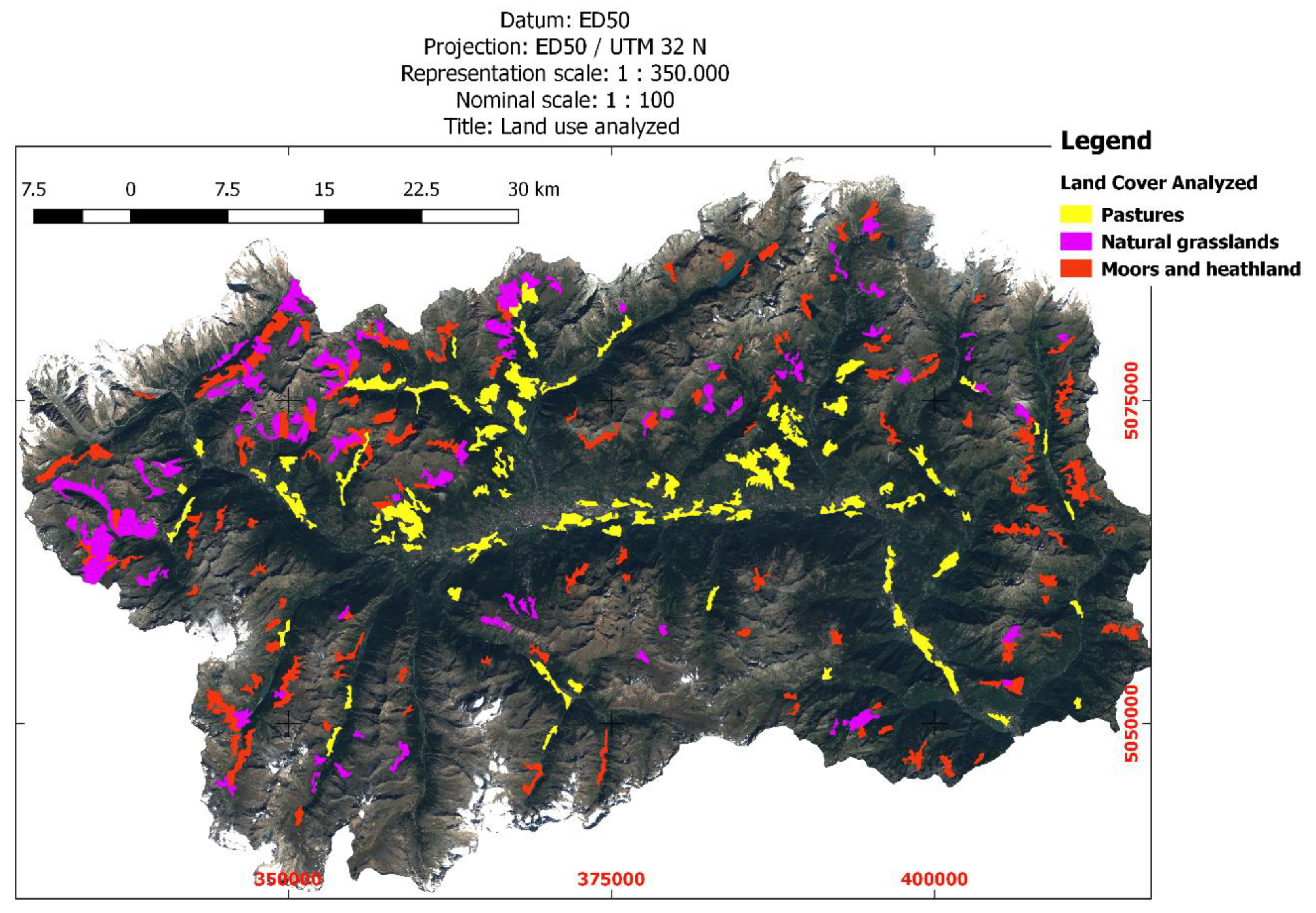
2.4. Land Cover Data
2.5. Methodology
- Analysis 1: testing PM and ET trends from NTS and ETS
- Analysis 2: IKC prevalence vs. PMs/ET
3. Results
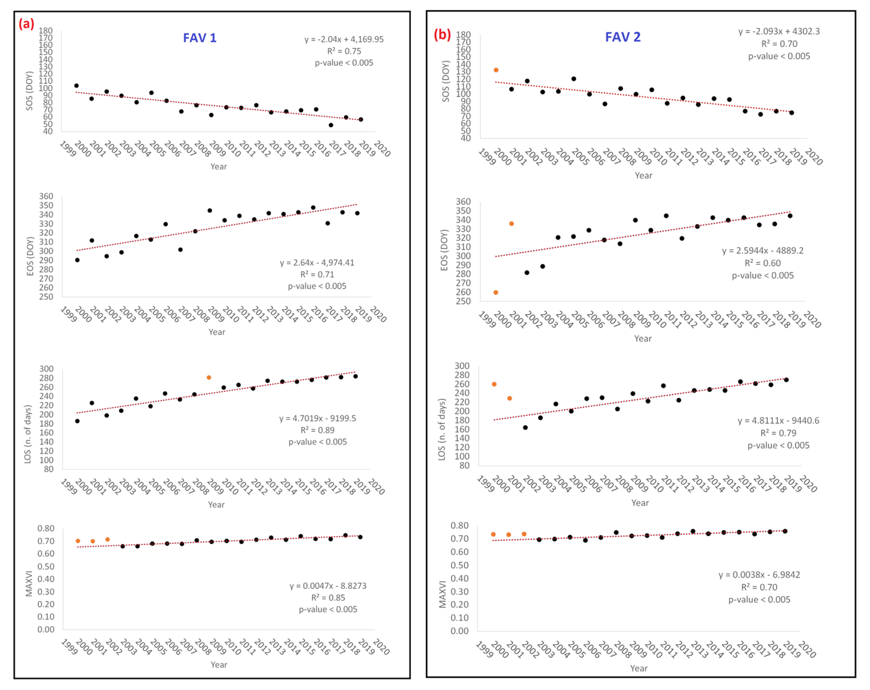
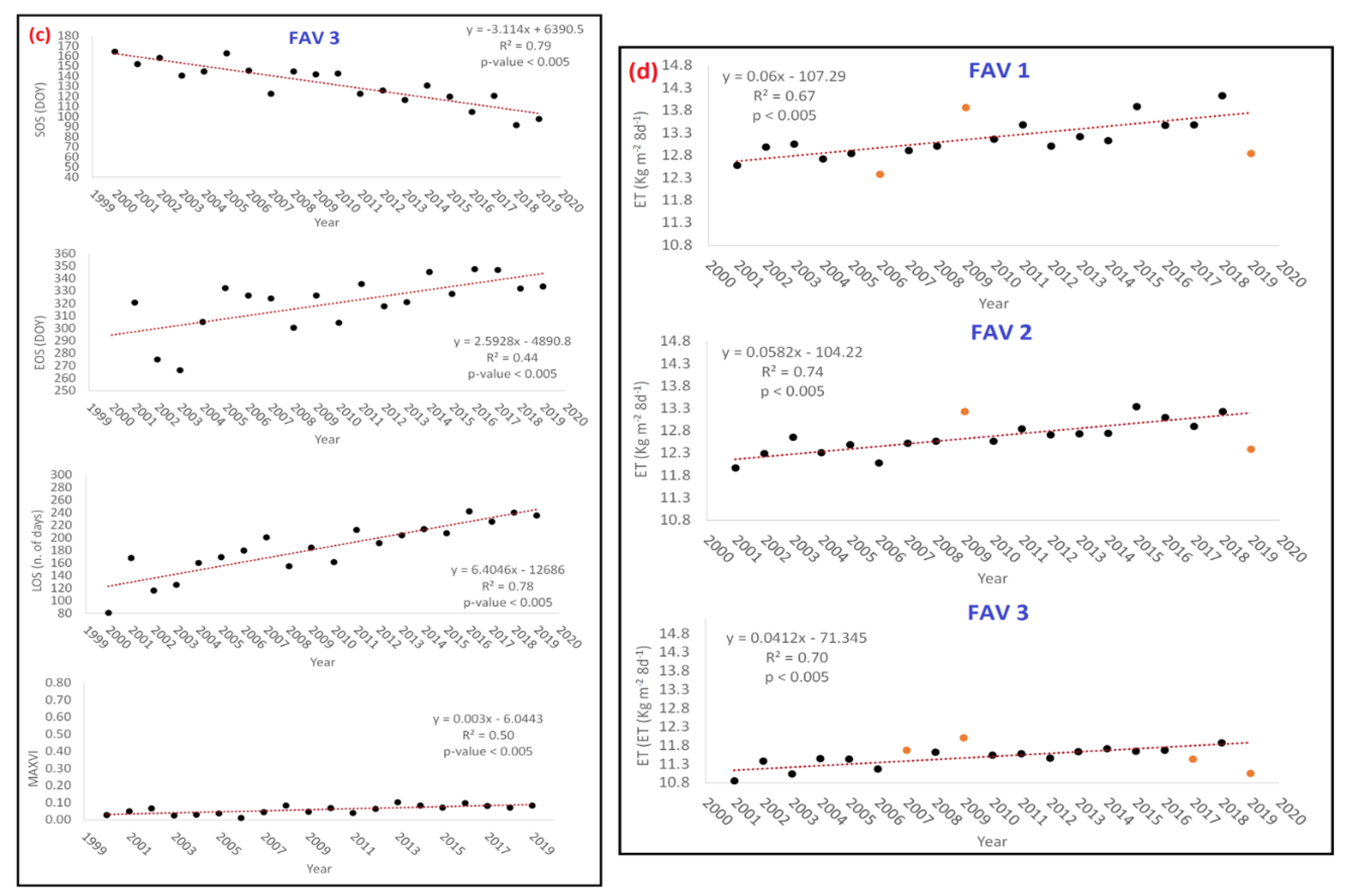
- Analysis 1: testing PM and ET trends from NTS and ETS
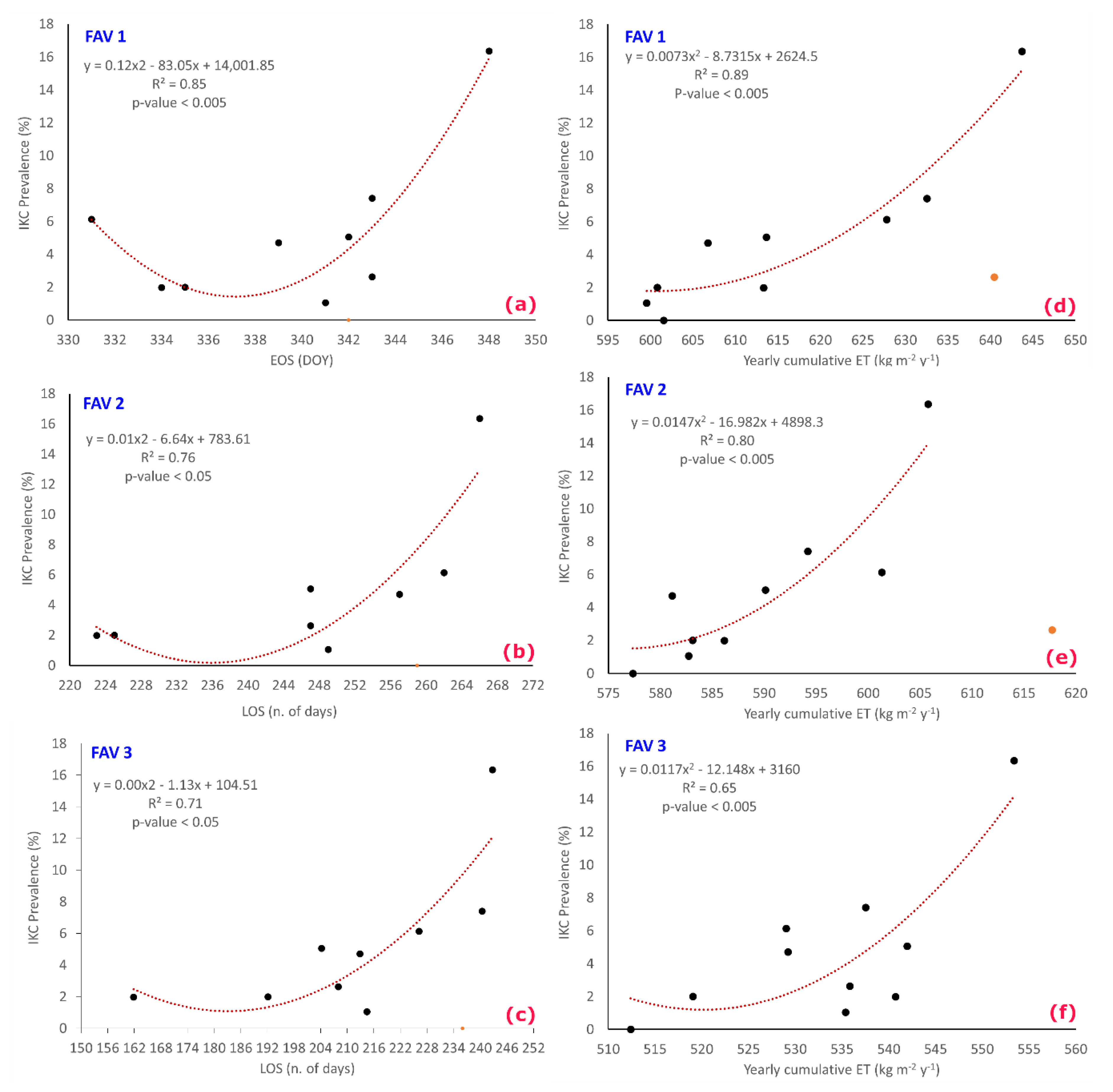
- Analysis 2: IKC prevalence vs. PMs/ET
4. Discussions
5. Conclusions
Author Contributions
Funding
Acknowledgments
Conflicts of Interest
Abbreviations
| Acronyms | Description |
| ASL | Local Sanitary Enterprise (translated) |
| CeRMAS | National Reference Center for Wildlife Diseases (Italy) |
| DISAFA | Department of Agricultural, Forest and Food Sciences |
| DOY | Day of Year |
| DTM | Digital Terrain Model |
| EO Data | Earth Observation Data |
| EOS | End of Season |
| ET | Evapotranspiration |
| ETS | Evapotranspiration Time Series |
| FAV | Altimetry band-class |
| GEE | Google Earth Engine |
| IKC | Infectious keratoconjunctivitis |
| IZS PLV | Istituto Zooprofilattico Sperimentale Piemonte Liguria e Valle d’Aosta |
| JPL | Jet Propulsion Laboratory |
| LOS | Length of Season |
| LST | Land Surface Temperature |
| MAXVI | Maximum of NDVI |
| NASA | National Aeronautics and Space Administration |
| NDVI | Normalized Difference Vegetation Index |
| NTS | NDVI Time Series |
| PCR | Polymerase Chain Reaction |
| PMs | Phenological metrics |
| Pr | Prevalence (of a disease) |
| RFD | Regional Forestry Districts |
| SOS | Start of Season |
| SRTM | Shuttle Radar Topography Mission |
| Unito | University of Turin |
| VDA | Aosta Valley |
References
- Hay, S.; Snow, R.; Rogers, D. From Predicting Mosquito Habitat to Malaria Seasons Using Remotely Sensed Data: Practice, Problems and Perspectives. Parasitol. Today 1998, 14, 306–313. [Google Scholar] [CrossRef]
- Hendrickx, G.; Biesemans, J.; De Deken, R. The use of GIS in veterinary parasitology. GIS Spat. Anal. Vet. Sci. 2009, 145–176. [Google Scholar] [CrossRef]
- Kazmi, S.J.H.; Usery, E.L. Application of remote sensing and gis for the monitoring of diseases: A unique research agenda for geographers. Remote Sens. Rev. 2001, 20, 45–70. [Google Scholar] [CrossRef]
- Durr, P.A.; Gatrell, A.C. (Eds.) GIS and spatial analysis in veterinary science. Cabi 2004, 1–33. [Google Scholar]
- Housman, I.W.; Chastain, R.A.; Finco, M.V. An Evaluation of Forest Health Insect and Disease Survey Data and Satellite-Based Remote Sensing Forest Change Detection Methods: Case Studies in the United States. Remote Sens. 2018, 10, 1184. [Google Scholar] [CrossRef] [Green Version]
- Correia, V.R.D.M.; Carvalho, M.S.; Sabroza, P.C.; Vasconcelos, C.H. Remote sensing as a tool to survey endemic diseases in Brazil. Cad. Saúde Pública 2004, 20, 891–904. [Google Scholar] [CrossRef] [Green Version]
- Kiang, R. Malaria Modeling and Surveillance. Benchmark Rep. 2009, 1–5. [Google Scholar]
- Anyamba, A.; Chretien, J.-P.; Britch, S.C.; Soebiyanto, R.P.; Small, J.L.; Jepsen, R.; Forshey, B.M.; Sanchez, J.L.; Smith, O.; Odette, M.; et al. Global Disease Outbreaks Associated with the 2015–2016 El Niño Event. Sci. Rep. 2019, 9, 1–14. [Google Scholar] [CrossRef] [Green Version]
- Kalluri, S.; Gilruth, P.; Rogers, D.; Szczur, M. Surveillance of Arthropod Vector-Borne Infectious Diseases Using Remote Sensing Techniques: A Review. PLoS Pathog. 2007, 3, e116. [Google Scholar] [CrossRef]
- Estrada-Peña, A.; Estrada-Sánchez, A.; De La Fuente, J. A global set of Fourier-transformed remotely sensed covariates for the description of abiotic niche in epidemiological studies of tick vector species. Parasites Vectors 2014, 7, 302. [Google Scholar] [CrossRef] [Green Version]
- Wang, J.; Jia, P.; Cuadros, D.F.; Xu, M.; Wang, X.; Guo, W.; Portnov, B.A.; Bao, Y.; Yu, S.; Song, G.; et al. A Remote Sensing Data Based Artificial Neural Network Approach for Predicting Climate-Sensitive Infectious Disease Outbreaks: A Case Study of Human Brucellosis. Remote Sens. 2017, 9, 1018. [Google Scholar] [CrossRef] [Green Version]
- Hartemink, N.; Vanwambeke, S.O.; Purse, B.V.; Gilbert, M.; Van Dyck, H. Towards a resource-based habitat approach for spatial modelling of vector-borne disease risks. Biol. Rev. 2014, 90, 1151–1162. [Google Scholar] [CrossRef] [PubMed] [Green Version]
- Olivero, J.; Fa, J.E.; Real, R.; Márquez, A.L.; Farfán, M.A.; Vargas, J.M.; Gaveau, D.; Salim, M.A.; Park, D.; Suter, J.; et al. Recent loss of closed forests is associated with Ebola virus disease outbreaks. Sci. Rep. 2017, 7, 1–9. [Google Scholar] [CrossRef] [PubMed] [Green Version]
- Robinson, R.A. Plant Pathosystems; Springer: Berlin/Heidelberg, Germany, 1976; pp. 15–31. [Google Scholar]
- Conticini, E.; Frediani, B.; Caro, D. Can atmospheric pollution be considered a co-factor in extremely high level of SARS-CoV-2 lethality in Northern Italy? Environ. Pollut. 2020, 261, 114465. [Google Scholar] [CrossRef]
- Rinaldi, L.; Musella, V.; Biggeri, A.; Cringoli, G. New insights into the application of geographical information systems and remote sensing in veterinary parasitology. Geospat. Health 2006, 1, 33. [Google Scholar] [CrossRef] [Green Version]
- Jebara, K.B. The role of Geographic Information System (GIS) in the control and prevention of animal diseases. Conf. OIE 2007, 1, 175–183. [Google Scholar]
- Barile, M.F.; Del Giudice, R.A.; Tully, J.G. Isolation and Characterization of Mycoplasma conjunctivae sp. n. from Sheep and Goats with Keratoconjunctivitis. Infect. Immun. 1972, 5, 70–76. [Google Scholar] [CrossRef] [Green Version]
- Giacometti, M.; Janovsky, M.; Jenny, H.; Nicolet, J.; Belloy, L.; Goldschmidt-Clermont, E.; Frey, J. Mycoplasma conjunctivae infection is not maintained in alpine chamois in eastern switzerland. J. Wildl. Dis. 2002, 38, 297–304. [Google Scholar] [CrossRef] [Green Version]
- Giangaspero, M.; Orusa, R.; Nicholas, R.A.; Harasawa, R.; Ayling, R.D.; Churchward, C.; Whatmore, A.M.; Bradley, D.; Robetto, S.; Sacchi, L.; et al. Characterization of mycoplasma isolated from an ibex (capra ibex) suffering from keratoconjunctivitis in northern italy. J. Wildl. Dis. 2010, 46, 1070–1078. [Google Scholar] [CrossRef]
- Degiorgis, M.P.; Frey, J.; Nicolet, J.; Abdo, E.M.; Fatzer, R.; Schlatter, Y.; Reist, S.; Janovsky, M.; Giacometti, M. An outbreak of infectious keratoconjunctivitis in Alpine chamois (Rupicapra r. rupicapra) in Simmental-Gruyères. Schweiz Arch Tierheilkd 2000, 142, 520–527. [Google Scholar]
- Grattarola, C.; Frem, E.M.; Orusa, R.; Nicolet, M.G. Ker’atoconjunctivitis in. Vet. Rec. 1999, 145, 588–589. [Google Scholar] [CrossRef] [PubMed]
- Giacometti, M.; Janovsky, M.; Belloy, L.; Frey, J. Infectious keratoconjunctivitis of ibex, chamois and other Caprinae. Rev. Sci. Tech. Off. Int. Epizoot. 2002, 21, 335–345. [Google Scholar] [CrossRef] [PubMed] [Green Version]
- Mavrot, F.; Vilei, E.M.; Marreros, N.; Signer, C.; Frey, J.; Ryser-Degiorgis, M.-P. Occurrence, quantification, and genotyping of Mycoplasma conjunctivae in wild caprinae with and without infectious keratoconjunctivitis. J. Wildl. Dis. 2012, 48, 619–631. [Google Scholar] [CrossRef] [PubMed]
- Hars, J.; Gauthier, D. Suivi de l’évolution de la kérato-conjonctivite sur le peuplement d’ongulés sauvages du Parc National de la Vanoise en 1983. Trav. Sci. Parc. Nat. Vanoise 1984, 14, 157–210. [Google Scholar]
- Tschopp, R.; Frey, J.; Zimmermann, L.; Giacometti, M. Outbreaks of infectious keratoconjunctivitis in alpine chamois and ibex in Switzerland between 2001 and 2003. Vet. Rec. 2005, 157, 13–18. [Google Scholar] [CrossRef]
- Nesti, I.; Posillico, M.; Lovari, S. Ranging behaviour and habitat selection of Alpine chamois. Ethol. Ecol. Evol. 2010, 22, 215–231. [Google Scholar] [CrossRef]
- Arnal, M.; Herrero, J.; De La Fe, C.; Revilla, M.; Prada, C.; Martínez-Durán, D.; Gómez-Martin, Á.; Fernández-Arberas, O.; Amores, J.; Contreras, A.; et al. Dynamics of an Infectious Keratoconjunctivitis Outbreak by Mycoplasma conjunctivae on Pyrenean Chamois Rupicapra p. pyrenaica. PLoS ONE 2013, 8, e61887. [Google Scholar] [CrossRef] [Green Version]
- Giangaspero, M.; Domenis, L.; Robetto, S.; Orusa, R. Histological and virological findings in severe meningoencephalitis associated with border disease virus in Alpine chamois (Rupicapra rupicapra rupicapra) in Aosta Valley, Italy. Open Vet. J. 2019, 9, 81–87. [Google Scholar] [CrossRef] [Green Version]
- Abbona, F.; Venturino, E. An eco-epidemic model for infectious keratoconjunctivitis caused by Mycoplasma conjunctivae in domestic and wild herbivores, with possible vaccination strategies. Math. Methods Appl. Sci. 2016, 41, 2269–2280. [Google Scholar] [CrossRef]
- Ambroselli, S. Istat working papers. ISTAT 2019, 24, 47–49. [Google Scholar]
- Rubel, F.; Brugger, K.; Haslinger, K.; Auer, I. The climate of the European Alps: Shift of very high resolution Köppen-Geiger climate zones 1800–2100. Meteorol. Z. 2017, 26, 115–125. [Google Scholar] [CrossRef]
- Sergio, F.; Pedrini, P. Biodiversity gradients in the Alps: The overriding importance of elevation. Biodivers. Conserv. 2007, 16, 3243–3254. [Google Scholar] [CrossRef] [Green Version]
- Fischer, M.; Rudmann-Maurer, K.; Weyand, A.; Stöcklin, J. Agricultural Land Use and Biodiversity in the Alps. Mt. Res. Dev. 2008, 28, 148–155. [Google Scholar] [CrossRef] [Green Version]
- Zimmermann, P.; Tasser, E.; Leitinger, G.; Tappeiner, U. Effects of land-use and land-cover pattern on landscape-scale biodiversity in the European Alps. Agric. Ecosyst. Environ. 2010, 139, 13–22. [Google Scholar] [CrossRef]
- Balestrieri, A.; Remonti, L.; Ferrari, N.; Ferrari, A.; Valvo, T.L.; Robetto, S.; Orusa, R. Sarcoptic mange in wild carnivores and its co-occurrence with parasitic helminths in the Western Italian Alps. Eur. J. Wildl. Res. 2006, 52, 196–201. [Google Scholar] [CrossRef]
- Renna, M.; Ravetto Enri, S.; Probo, M.; Lussiana, C.; Malfatto, V.; Battaglini, L.M.; Lonati, M.; Lombardi, G. Alpine grasslands: Relations among botanical and chemical variables affecting animal product quality. In Proceedings of the 19th Meeting of the FAO CIHEAM Mountain Pastures Network–Mountain Pastures and Livestock Farming Facing Uncertainty: Environmental, Technical and Socio-Economic Challenges, Zaragoza, Spain, 14–16 June 2016. [Google Scholar]
- Cavallero, A.; Aceto, P.; Gorlier, A.; Lombardi, G.; Lonati, M.; Martinasso, B.; Tagliatori, C. I Tipi Pastorali Delle Alpi Piemontesi; Alberto Perdisia Editore Divisione Università: Bologna, Italy, 2007; pp. 1–467. [Google Scholar]
- Probo, M.; Lonati, M.; Pittarello, M.; Bailey, D.W.; Garbarino, M.; Gorlier, A.; Lombardi, G. Implementation of a rotational grazing system with large paddocks changes the distribution of grazing cattle in the south-western Italian Alps. Rangel. J. 2014, 36, 445–458. [Google Scholar] [CrossRef] [Green Version]
- Zimmermann, L.; Jambresic, S.; Giacometti, M.; Frey, J. Specificity of Mycoplasma conjunctivae strains for alpine chamois Rupicapra r. rupicapra. Wildl. Biol. 2008, 14, 118–124. [Google Scholar] [CrossRef]
- Vilei, E.M.; Bonvin-Klotz, L.; Zimmermann, L.; Ryser-Degiorgis, M.-P.; Giacometti, M.; Frey, J. Validation and diagnostic efficacy of a TaqMan real-time PCR for the detection of Mycoplasma conjunctivae in the eyes of infected Caprinae. J. Microbiol. Methods 2007, 70, 384–386. [Google Scholar] [CrossRef]
- Belloy, L.; Janovsky, M.; Vilei, E.M.; Pilo, P.; Giacometti, M.; Frey, J. Molecular Epidemiology of Mycoplasma conjunctivae in Caprinae: Transmission across Species in Natural Outbreaks. Appl. Environ. Microbiol. 2003, 69, 1913–1919. [Google Scholar] [CrossRef] [Green Version]
- Didan, K. MOD13Q1 MODIS/Terra Vegetation Indices 16-Day L3 Global 250m SIN Grid V006 [Data set]. NASA EOSDIS Land Processes DAAC. Available online: https://0-doi-org.brum.beds.ac.uk/10.5067/MODIS/MOD13Q1.006 (accessed on 28 April 2020).
- Gorelick, N.; Hancher, M.; Dixon, M.; Ilyushchenko, S.; Thau, D.; Moore, R. Google Earth Engine: Planetary-scale geospatial analysis for everyone. Remote Sens. Environ. 2017, 202, 18–27. [Google Scholar] [CrossRef]
- Schafer, R.W. What Is a Savitzky-Golay Filter? [Lecture Notes]. IEEE Signal Process. Mag. 2011, 28, 111–117. [Google Scholar] [CrossRef]
- Press, W.H.; Teukolsky, S.A. Savitzky-Golay Smoothing Filters. Comput. Phys. 1990, 4, 669. [Google Scholar] [CrossRef]
- O’Connor, A.; Lausten, K.; Okubo, B.; Harris, T. ENVI Services Engine: Earth and planetary image processing for the cloud. Am. Geophys. Union Poster IN21C-1490 2012, 45, 34–49. [Google Scholar]
- Running, S.; Mu, Q.; Zhao, M. MOD16A2 MODIS/Terra Net Evapotranspiration 8-Day L4 Global 500m SIN Grid V006 NASA EOSDIS Land Processes DAAC. EGU 2017. [Google Scholar] [CrossRef]
- Cai, J.; Liu, Y.; Lei, T.; Pereira, L.S. Estimating reference evapotranspiration with the FAO Penman–Monteith equation using daily weather forecast messages. Agric. For. Meteorol. 2007, 145, 22–35. [Google Scholar] [CrossRef]
- Leuning, R.; Zhang, Y.Q.; Rajaud, A.; Cleugh, H.; Tu, K. A simple surface conductance model to estimate regional evaporation using MODIS leaf area index and the Penman-Monteith equation. Water Resour. Res. 2008, 44. [Google Scholar] [CrossRef]
- Orusa, T.; Mondino, E.B. Landsat 8 thermal data to support urban management and planning in the climate change era: A case study in Torino area, NW Italy. Remote Sens. Technol. Appl. Urban Environ. IV 2019, 11157. [Google Scholar] [CrossRef]
- Farr, T.G.; Rosen, P.A.; Caro, E.; Crippen, R.; Duren, R.; Hensley, S.; Kobrick, M.; Paller, M.; Rodriguez, E.; Roth, L.; et al. The Shuttle Radar Topography Mission. Rev. Geophys. 2007, 45. [Google Scholar] [CrossRef] [Green Version]
- Werner, M. Shuttle Radar Topography Mission (SRTM) Mission Overview. Frequenz 2001, 55, 75–79. [Google Scholar] [CrossRef]
- Bossard, M.; Feranec, J.; Otahel, J. CORINE land cover technical guide: Addendum 2000. Researchgate 2000, 40, 1–105. [Google Scholar]
- Büttner, G.; Feranec, J.; Jaffrain, G.; Mari, L.; Maucha, G.; Soukup, T. The CORINE land cover 2000 project. EARSeL eProc. 2004, 3, 331–346. [Google Scholar]
- Available online: https://developers.google.com/earth-engine/datasets/catalog/COPERNICUS_CORINE_V20_100m (accessed on 1 January 2019).
- Hammer, Ø.; Harper, D.A.; Ryan, P.D. PAST: Paleontological statistics software package for education and data analysis. Palaeontol. Electron. 2001, 4, 9. [Google Scholar]
- QGIS Delopment Team. QGIS geographic information system. Open Source Geospat. Found. Project 2016, 1, 59. [Google Scholar]
- Conrad, O.; Bechtel, B.; Bock, M.; Dietrich, H.; Fischer, E.; Gerlitz, L.; Wehberg, J.; Wichmann, V.; Böhner, J. System for Automated Geoscientific Analyses (SAGA) v. 2.1.4. Geosci. Model Dev. 2015, 8, 1991–2007. [Google Scholar] [CrossRef] [Green Version]
- Sarvia, F.; De Petris, S.; Mondino, E.B. Multi-scale remote sensing to support insurance policies in agriculture: From mid-term to instantaneous deductions. GIScience Remote Sens. 2020, 57, 770–784. [Google Scholar] [CrossRef]
- Jönsson, P.; Eklundh, L. TIMESAT—A program for analyzing time-series of satellite sensor data. Comput. Geosci. 2004, 30, 833–845. [Google Scholar] [CrossRef] [Green Version]
- Tan, B.; Morisette, J.T.; Wolfe, R.E.; Gao, F.; Ederer, G.A.; Nightingale, J.; Pedelty, J.A. An Enhanced TIMESAT Algorithm for Estimating Vegetation Phenology Metrics from MODIS Data. IEEE J. Sel. Top. Appl. Earth Obs. Remote Sens. 2010, 4, 361–371. [Google Scholar] [CrossRef]
- Eklundh, L.; Jönsson, P. A new spatio-temporal smoother for extracting vegetation seasonality with TIMESAT. In Proceedings of the 35th International Symposium on Remote Sensing of Environment, Beijing, China, 22–26 April 2013. [Google Scholar]
- Cleveland, R.B.; Cleveland, W.S.; McRae, J.E.; Terpenning, I. STL: A seasonal-trend decomposition. J. Off. Stat. 1990, 6, 3–73. [Google Scholar]
- Jia, K.; Liang, S.; Wei, X.; Yao, Y.; Su, Y.; Jiang, B.; Wang, X. Land Cover Classification of Landsat Data with Phenological Features Extracted from Time Series MODIS NDVI Data. Remote Sens. 2014, 6, 11518–11532. [Google Scholar] [CrossRef] [Green Version]
- Borgogno-Mondino, E.; Lessio, A.; Gomarasca, M.A. A fast operative method for NDVI uncertainty estimation and its role in vegetation analysis. Eur. J. Remote Sens. 2016, 49, 137–156. [Google Scholar] [CrossRef]
- Cremonese, E.; Filippa, G.; Galvagno, M.; Siniscalco, C.; Oddi, L.; Di Cella, U.M.; Migliavacca, M. Heat wave hinders green wave: The impact of climate extreme on the phenology of a mountain grassland. Agric. For. Meteorol. 2017, 247, 320–330. [Google Scholar] [CrossRef]
- Migliavacca, M.; Galvagno, M.; Cremonese, E.; Rossini, M.; Meroni, M.; Sonnentag, O.; Cogliati, S.; Manca, G.; Diotri, F.; Busetto, L.; et al. Using digital repeat photography and eddy covariance data to model grassland phenology and photosynthetic CO2 uptake. Agric. For. Meteorol. 2011, 151, 1325–1337. [Google Scholar] [CrossRef]
- Julitta, T.; Cremonese, E.; Migliavacca, M.; Colombo, R.; Galvagno, M.; Siniscalco, C.; Rossini, M.; Fava, F.; Cogliati, S.; Di Cella, U.M.; et al. Using digital camera images to analyse snowmelt and phenology of a subalpine grassland. Agric. For. Meteorol. 2014, 198–199, 116–125. [Google Scholar] [CrossRef]
- Migliavacca, M.; Reichstein, M.; Richardson, A.D.; Mahecha, M.D.; Cremonese, E.; Delpierre, N.; Galvagno, M.; Law, B.E.; Wohlfahrt, G.; Black, T.A.; et al. Influence of physiological phenology on the seasonal pattern of ecosystem respiration in deciduous forests. Glob. Chang. Biol. 2014, 21, 363–376. [Google Scholar] [CrossRef]
- Colombo, R.; Busetto, L.; Fava, F.; Di Mauro, B.; Migliavacca, M.; Cremonese, E.; Galvagno, M.; Rossini, M.; Meroni, M.; Cogliati, S.; et al. Phenological monitoring of grassland and larch in the Alps from Terra and Aqua MODIS images. Ital. J. Remote Sens. 2011, 83–96. [Google Scholar] [CrossRef]
- Colombo, R.; Busetto, L.; Migliavacca, M.; Cremonese, E.; Meroni, M.; Galvagno, M.; Rossini, M.; Siniscalco, C.; Di Cella, U.M. On the spatial and temporal variability of Larch phenological cycle in mountainous areas. Ital. J. Remote Sens. 2009, 41, 79–96. [Google Scholar] [CrossRef]
- Filippa, G.; Cremonese, E.; Galvagno, M.; Migliavacca, M.; Di Cella, U.M.; Petey, M.; Siniscalco, C. Five years of phenological monitoring in a mountain grassland: Inter-annual patterns and evaluation of the sampling protocol. Int. J. Biometeorol. 2015, 59, 1927–1937. [Google Scholar] [CrossRef]
- Diolaiuti, G.A.; Bocchiola, D.; Vagliasindi, M.; D’Agata, C.; Smiraglia, C. The 1975–2005 glacier changes in Aosta Valley (Italy) and the relations with climate evolution. Prog. Phys. Geogr. Earth Environ. 2012, 36, 764–785. [Google Scholar] [CrossRef]
- Haeberli, W.; Hoelzle, M.; Paul, F.; Zemp, M. Integrated monitoring of mountain glaciers as key indicators of global climate change: The European Alps. Ann. Glaciol. 2007, 46, 150–160. [Google Scholar] [CrossRef] [Green Version]
- Calanca, P.; Roesch, A.; Jasper, K.; Wild, M. Global Warming and the Summertime Evapotranspiration Regime of the Alpine Region. Clim. Chang. 2006, 79, 65–78. [Google Scholar] [CrossRef]
- Goulden, M.L.; Bales, R.C. Mountain runoff vulnerability to increased evapotranspiration with vegetation expansion. Proc. Natl. Acad. Sci. USA 2014, 111, 14071–14075. [Google Scholar] [CrossRef] [Green Version]
- Steffen, W.; Richardson, K.; Rockström, J.; Cornell, S.E.; Fetzer, I.; Bennett, E.M.; Biggs, R.; Carpenter, S.R.; De Vries, W.; De Wit, C.A.; et al. Planetary boundaries: Guiding human development on a changing planet. Science 2015, 347, 1259855. [Google Scholar] [CrossRef] [PubMed] [Green Version]
- Rockström, J.; Steffen, W.; Noone, K.; Persson, Å.; Chapin, F.S.I.; Lambin, E.; Lenton, T.M.; Scheffer, M.; Folke, C.; Schellnhuber, H.J. Planetary Boundaries: Exploring the Safe Operating Space for Humanity. Ecol. Soc. 2009, 14. [Google Scholar] [CrossRef]
- O’Neill, D.W.; Fanning, A.L.; Lamb, W.F.; Steinberger, J.K. A good life for all within planetary boundaries. Nat. Sustain. 2018, 1, 88–95. [Google Scholar] [CrossRef] [Green Version]
- Cardinale, B.J.; Duffy, J.E.; Gonzalez, A.; Hooper, D.U.; Perrings, C.; Venail, P.; Narwani, A.; Mace, G.M.; Tilman, D.; Wardle, D.A.; et al. Biodiversity loss and its impact on humanity. Nat. Cell Biol. 2012, 486, 59–67. [Google Scholar] [CrossRef] [PubMed]


| Altitude Ranges (m a.s.l.) | Area (km2) | Area (%) |
|---|---|---|
| 343–500 | 6.6 | 0.2 |
| 500–1000 | 236.4 | 7.2 |
| 1000–1500 | 372.7 | 11.4 |
| 1500–2000 | 669.9 | 20.5 |
| 2000–2500 | 994.6 | 30.5 |
| 2500–3000 | 768.3 | 23.6 |
| 3000–3500 | 176.6 | 5.4 |
| 3500–4810 | 35.5 | 1.1 |
| CLC2018 Class Code | Description | Area (km2) | Area (%) | CLC2018 Class Code | Description | Area (km2) | Area (%) |
|---|---|---|---|---|---|---|---|
| 111 | Continuous urban fabric | 1.56 | 0.05 | 311 | Broad-leaved forest | 58.12 | 1.78 |
| 112 | Discontinuous urban fabric | 35.27 | 1.08 | 312 | Coniferous forest | 577.98 | 17.71 |
| 121 | Industrial or commercial units | 8.72 | 0.27 | 313 | Mixed forest | 104.41 | 3.20 |
| 122 | Road and rail networks and associated land | 0.25 | 0.01 | 321 | Natural grasslands | 86.04 | 2.64 |
| 124 | Airports | 0.42 | 0.01 | 322 | Moors and heathland | 106.29 | 3.26 |
| 131 | Mineral extraction sites | 0.66 | 0.02 | 324 | Transitional woodland-shrub | 424.84 | 13.02 |
| 132 | Dump sites | 0.27 | 0.01 | 332 | Bare rocks | 652.61 | 20.00 |
| 212 | Permanently irrigated land | 0.27 | 0.01 | 333 | Sparsely vegetated areas | 804.78 | 24.67 |
| 221 | Vineyards | 3.57 | 0.11 | 335 | Glaciers and permanent snow | 129.56 | 3.97 |
| 222 | Fruit trees and berry plantations | 2.17 | 0.07 | 411 | Inland marshes | 0.54 | 0.02 |
| 231 | Pastures | 94.06 | 2.88 | 511 | River | 0.17 | 0.01 |
| 242 | Complex cultivation patterns | 18.61 | 0.57 | 512 | Lakes | 3.24 | 0.10 |
| 243 | Land principally occupied by agriculture, with significant areas of natural vegetation | 148.42 | 4.55 |
| Class Code | Altitude Range (m) |
|---|---|
| FAV1 | <1000 |
| FAV2 | 1000–2000 |
| FAV3 | 2000–3000 |
| Year 1 | Year Analyzed 2 | IKC Disease Prevalence (%) | Number of Samples Analyzed | Positive to IKC |
|---|---|---|---|---|
| 2009–2010 | 2010 | 2.0 | 302 | 6 |
| 2010–2011 | 2011 | 4.7 | 191 | 9 |
| 2011–2012 | 2012 | 2.0 | 150 | 3 |
| 2012–2013 | 2013 | 5.1 | 158 | 8 |
| 2013–2014 | 2014 | 1.1 | 190 | 2 |
| 2014–2015 | 2015 | 2.6 | 152 | 4 |
| 2015–2016 | 2016 | 16.4 | 159 | 26 |
| 2016–2017 | 2017 | 6.1 | 114 | 7 |
| 2017–2018 | 2018 | 7.4 | 108 | 8 |
| 2018–2019 | 2019 | 0.0 | 100 | 0 |
| Yearly | SOS (DOY) | EOS (DOY) | LOS (n. of Days) | MAXVI | ET (kg·m−2·8 d−1) |
| FAV1 | −2.04 | 2.64 | 4.70 | 0.005 | 0.06 |
| FAV2 | −2.09 | 2.59 | 4.81 | 0.004 | 0.04 |
| FAV3 | −3.11 | 2.59 | 6.40 | 0.003 | 0.06 |
| Cumulated 2000–2019 | SOS (DOY) | EOS (DOY) | LOS (n. of Days) | MAXVI | ET (Kg m−2) |
| FAV1 | −38.76 | 50.16 | 89.34 | 0.089 | 1.14 |
| FAV2 | −39.77 | 49.29 | 91.41 | 0.072 | 0.78 |
| FAV3 | −59.17 | 49.26 | 121.69 | 0.057 | 1.11 |
| Classes | SOS | EOS | LOS | MAXVI | Yearly Cumulative ET | |||||
|---|---|---|---|---|---|---|---|---|---|---|
| R2 | p-Value | R2 | p-Value | R2 | p-Value | R2 | p-Value | R2 | p-Value | |
| FAV1 | 0.06 | 0.83 | 0.85 | 0.003 * | 0.26 | 0.41 | 0.06 | 0.90 | 0.89 | 0.004 * |
| FAV2 | 0.51 | 0.11 | 0.13 | 0.65 | 0.76 | 0.01 * | 0.16 | 0.68 | 0.80 | 0.005 * |
| FAV3 | 0.46 | 0.16 | 0.28 | 0.35 | 0.71 | 0.02 * | 0.31 | 0.32 | 0.65 | 0.003 * |
Publisher’s Note: MDPI stays neutral with regard to jurisdictional claims in published maps and institutional affiliations. |
© 2020 by the authors. Licensee MDPI, Basel, Switzerland. This article is an open access article distributed under the terms and conditions of the Creative Commons Attribution (CC BY) license (http://creativecommons.org/licenses/by/4.0/).
Share and Cite
Orusa, T.; Orusa, R.; Viani, A.; Carella, E.; Borgogno Mondino, E. Geomatics and EO Data to Support Wildlife Diseases Assessment at Landscape Level: A Pilot Experience to Map Infectious Keratoconjunctivitis in Chamois and Phenological Trends in Aosta Valley (NW Italy). Remote Sens. 2020, 12, 3542. https://0-doi-org.brum.beds.ac.uk/10.3390/rs12213542
Orusa T, Orusa R, Viani A, Carella E, Borgogno Mondino E. Geomatics and EO Data to Support Wildlife Diseases Assessment at Landscape Level: A Pilot Experience to Map Infectious Keratoconjunctivitis in Chamois and Phenological Trends in Aosta Valley (NW Italy). Remote Sensing. 2020; 12(21):3542. https://0-doi-org.brum.beds.ac.uk/10.3390/rs12213542
Chicago/Turabian StyleOrusa, Tommaso, Riccardo Orusa, Annalisa Viani, Emanuele Carella, and Enrico Borgogno Mondino. 2020. "Geomatics and EO Data to Support Wildlife Diseases Assessment at Landscape Level: A Pilot Experience to Map Infectious Keratoconjunctivitis in Chamois and Phenological Trends in Aosta Valley (NW Italy)" Remote Sensing 12, no. 21: 3542. https://0-doi-org.brum.beds.ac.uk/10.3390/rs12213542