Experimental Fire Measurement with UAV Multimodal Stereovision


Campus Grimaldi, Université de Corse, UMR CNRS 6134 SPE, 20250 Corte, France
*
Author to whom correspondence should be addressed.
Remote Sens. 2020, 12(21), 3546; https://0-doi-org.brum.beds.ac.uk/10.3390/rs12213546
Submission received: 15 October 2020
/
Revised: 23 October 2020
/
Accepted: 27 October 2020
/
Published: 29 October 2020
(This article belongs to the Special Issue Latest Developments in 3D Mapping with Unmanned Aerial Vehicles)
Abstract
:In wildfire research, systems that are able to estimate the geometric characteristics of fire, in order to understand and model the behavior of this spreading and dangerous phenomenon, are required. Over the past decade, there has been a growing interest in the use of computer vision and image processing technologies. The majority of these works have considered multiple mono-camera systems, merging the information obtained from each camera. Recent studies have introduced the use of stereovision in this field; for example, a framework with multiple ground stereo pairs of cameras has been developed to measure fires spreading for about 10 meters. This work proposes an unmanned aerial vehicle multimodal stereovision framework which allows for estimation of the geometric characteristics of fires propagating over long distances. The vision system is composed of two cameras operating simultaneously in the visible and infrared spectral bands. The main result of this work is the development of a portable drone system which is able to obtain georeferenced stereoscopic multimodal images associated with a method for the estimation of fire geometric characteristics. The performance of the proposed system is tested through various experiments, which reveal its efficiency and potential for use in monitoring wildfires.

1. Introduction
Every year, wildfires cause ecological, economic, and human disasters [1]. The term “wildfires”— also known as “forest fires” or “wildland fires”, is commonly used to refer to unwanted fires that burn forests and wildlands [2,3]. Annually, more than 340 million hectares of vegetation are burned on our planet by these fires [4]. Climate and weather are some of the major factors increasing wildfire hazard and risk [5]. In the near future, global temperatures are expected to be warmer than current levels, severe droughts to be more frequent, and fire seasons to be longer in many ecosystems. Other anthropogenic factors have contributed to the increase in fire risk worldwide [2,6]; for instance, anarchic extension of the urbanization in wildland–urban interfaces (WUIs) or fire exclusion policies, which contribute to fuel accumulation, can potentially increase the impacts of wildfires. With the combination of these factors, wildfires may occur more frequently. This evolving scenario requires strategies that are able to reduce the risk of fires and thereby decrease their economic, environmental, and social impacts. Therefore, management, prevention, and control actions are performed. The effectiveness of these types of actions is related to the knowledge of the phenomena that occur during the outbreak and spread of fire. Wildfire research has been conducted for more than 50 years, in order to understand these phenomena, to develop propagation and behavior models, to predict the evolution of wildfires [7,8,9,10,11] and the heat they transfer [12,13,14], and to develop decision management systems for fire fighting and land-use planning [15,16,17,18,19].
Experimental data of fire spread across vegetal fuels in laboratory and field conditions are needed to better understand the phenomenon and improve and/or validate models. Fire front characteristics such as position, rate of spread, base area, height, length, width, depth, inclination, shape, surface, and volume are needed. Three-dimensional (3D) information are as complete as can be expected. Thus, for example, all the points of a non-linear fire front could be monitored, which indicate fire front deformation, which can occur due to terrain topology, wind, or vegetation. The energy transferred from a fire to a target depends on the distance between the target, as well as the fire and the orientation of the fire surface in relation to the position of the target [20]. Obtaining the 3D shape of a fire and having, at each instant, the distance from the fire to the target and the surface of the flame that is oriented toward the target allows for the estimation of this energy. In recent decades, research activity in the fire community has focused on developing methods based on computer vision to measure the geometric characteristics of propagating fire. The step of detection of fire pixels in an image is essential in the process of measuring fire by vision, as it determines the accuracy with which the characteristics of the phenomenon can be estimated. The visible domain is the reference spectrum used by researchers working on wildfires, due to the simplicity of use of visible cameras and their affordable price. However, the detection of fire pixels in an image representing the visible spectrum is challenging and it appears [21] that the performance of 11 state-of-the-art fire color segmentation algorithms [22,23,24,25,26,27,28,29,30,31,32] (benchmarked using a data set containing more than 500 wildfire images [33]) are dependent on the features of the fire, including, for instance, color, texture, presence of smoke, and luminosity of the background. The use of infrared images can help to overcome the problem of fires masked by smoke. Multiple works have been conducted in this area. Gouverneur et al. [34] found that the best spectral bands for fire detection (long-distance fire camera) were short wavelength infrared (SWIR: –3 m), middle wavelength infrared (MWIR: 3–5 m), and long wavelength infrared (LWIR: 8–15 m). However, as the fire emits in several spectral bands in a non-uniform way, the fire areas obtained from different spectral images do not perfectly overlap. This is due to some hot gas zones not being captured by the visible spectrum [34,35]. Thus, infrared images alone cannot be used for measuring the geometric characteristics of fires.
Systems using multiple modalities have been proposed: Verstockt et al. [36] proposed the use of a system that combines LWIR and visible spectrum sensors, as well as a system that uses time of flight (TOF) and visible sensors [37]. In these latest studies, the experiments were limited to controlled environments. As the resolutions of the cameras used in these studies were low, they cannot be used for fire metrology.
For the development of a vision-based measurement system dedicated to fires, two kinds of frameworks have been developed: The first uses mono-cameras which are positioned to obtain complementary views [38,39,40,41], but is not applicable in an uncontrolled environment. Martínez-de-Dios et al. [42] developed a vision-based measurement system at the field scale using fixed cameras positioned at two viewpoints (frontal and lateral views) to obtain complementary information. Frontal images allow for the estimation of fire front position and the rate of spread, while lateral cameras are useful for extracting the maximum flame height, the flame inclination, and the fire base width. An infrared camera is also deployed in a lateral position, in order to obtain the fire location and the fire base width for situations with smoke present, which masks visual images. Real-world estimations of fire features are computed by calibrating the cameras using a terrain model, camera position, and artificial beacons and natural marks. The developed system was used to estimate the position of the most advanced point of the fire front and its width. Finally, a 3D view of the fire model is generated using the computed measurements. Other authors have proposed improvements of this method using visual and infrared cameras fixed on the ground or mounted onboard unmanned aerial systems with a differential global positioning system (GPS) and inertial measurement units (IMU), using data fusion techniques to integrate the results from the different cameras [43]. This framework can be used to estimate the location of the fire front, the rate of spread, and the maximum height of the flames in real time. The 3D fire shape is obtained by the concatenation of triangles, each of which is characterized by the estimated features. This system estimates part of the geometric characteristics needed by researchers working on forest fire propagation and behavior modeling. However, when using 2D information, 3D depth information cannot be obtained for all the points of a fire front and, therefore, certain characteristics cannot be estimated. Moreover, deployment can be challenging in areas that are difficult to access.
The second family of frameworks is based on the use of stereovision to compute 3D information [44]. This method obtains depth information from two simultaneous and staggered images of the same scene without the need for landmarks or artificial beacons. It has been applied at the laboratory scale to measure the geometric characteristics of a fire front [45,46]. A system was also developed for the semi-field scale [47]. The framework supports the use of multiple stereo pairs which are positioned to capture complementary views of the fire front during its propagation. Multimodal stereo pairs operating in both the visible and near-infrared spectral bands are used. Each of the cameras forming the stereo pair is rigidly fixed on a metallic bar with a one meter baseline. This baseline value, which is associated to the focal length that is used and with a camera–fire distance of 15 m, produces a theoretical precision of depth measurement of less than 0.3 m.
Registration is conducted using the captured views to build a complete 3D reconstruction of the fire front. This is achieved using multisensory fusion based on visual data, GPS positions, and IMU inertial data. This framework effectively estimates the geometric characteristics of a fire propagating in a field of about 10 m over time: position, rate of spread, base width, depth, perimeter, height, length, flame inclination angle, 3D shape, surface, view factor, and volume. However, it has certain limitations: First, it is necessary to anticipate the fire path, in order to optimally position the cameras. Second, as the theoretical precision of the depth measurement increases proportionally to the square of the camera–object distance [48], precision loss occurs when the fire moves away from the cameras. The use of a stereovision system carried by an unmanned aerial vehicle (UAV) can overcome these problems, as the drone can stay close to the fire throughout its evolution. The first challenge to be met when using a vison system whose position and orientation change at every moment is expressing the data in a global reference frame. The second is computing the equation of the local propagation plane of the fire and its main direction for each image acquisition instant, which are necessary for the estimation of the geometric characteristics.
This paper presents a UAV multimodal stereovision system for the measurement of the geometric characteristics of fires propagating over unlimited distances. It is based on our previous work in the area of 3D vision-based metrology of fires [47,49]. A vision device that is fixable on a UAV, composed of two cameras operating simultaneously in the visible and the infrared ranges, and able to produce georeferenced stereoscopic multimodal images is presented. The proposed framework permits the estimation of the 3D shape of the fire front, its position on the ground, rate of spread, surface, thickness, height, and inclination angle for any terrain configuration and without using a digital terrain model. To evaluate the performance of the system, tests were conducted with experimental fires spreading over several tens of meters on terrains with variable slope.
2. Materials and Methods
2.1. Multimodal Stereovision System
The stereovision system is composed by two FLIR Duo Pro R 640 cameras (FLIR Systems Inc, Wilsonville, OR, USA) [50] rigidly fixed on a carbon fiber draping axis with an inter-camera distance of 0.85 m, which is attached to a Matrice 600 Pro DJI UAV (DJI, Shenzhen, China) (Figure 1).
The camera combines an FLIR Tau 2 thermal sensor and a 4K sensor, such that images in the visible and LWIR spectra are taken simultaneously. The visible sensor has a focal length of 8 mm with a pixel resolution of pixels and a field of view of . The infrared sensor has a focal length of 13 mm with a pixel resolution of and a field of view of . The maximum frame rate of the camera is 30 Hz but, for researchers working on fire behavior modeling, the frequency of 1/4 frames per second (fps) is generally considered adequate and, so, we decided to set it to this value. Simultaneous image acquisition by the two FLIR Duo Pro R cameras is triggered using an external 50 fps pulse width modulation (PWM) signal generated by a Raspberry Pi 2B+ (Newark Corporation, Chicago, IL, USA) computer, which is also used to store the data; the images are processed offline. A 3S 500 mAh LiPo battery and a power bank are used to power the cameras and the computer, respectively; they are fixed on the drone chassis, near its center of gravity. The total weight of the vision system, integrating the cameras, batteries, and the Raspberry computer, is 2.278 kg.
The theoretical precision of depth measurement () in a stereo system is linked to the precision of the disparity measurement () by:
where is the disparity in pixels, z is the real distance between the object and the stereovision system in meters, B is the baseline of the stereovision system in meters, and f is the focal length of the cameras in pixels. Considering m, and m, the theoretical precision of the depth measurement () of the stereovision system composed by the visible sensors is 0.4 m. This value is 1.7 m if the distance between the UAV and the fire is 30 m.
The stereovision system was calibrated outdoors using a m checkerboard formed of black and white square patterns. The white squares were covered with aluminium to obtain information in the visible and IR domains. Calibration was performed using Bouguet’s MATLAB (MathWorks, Natick, MA, USA) calibration toolbox [51], which permits the extraction of intrinsic and extrinsic parameters that are used in the stereo image rectification process.
The FLIR Duo Pro R camera integrates an onboard GPS/compass sensor, IMU board, and altitude sensors. These sensors are used to obtain the position and orientation of the vision system at each instant and generate georeferenced images.
2.2. Methodology
A diagram of the proposed methodology is shown in Figure 2. The first step of the process consists of detecting the fire pixels, which is conducted in both the LWIR spectrum and the visible range. Then, the visible picture is analyzed such that the most important feature points can be implemented in the stereo matching algorithm. From the corresponding points, a triangulation procedure permits their 3D reconstruction. At each image acquisition time, the field local plane equation is estimated using the lower 3D fire points. The 3D fire points are then projected in several frames to produce results expressed in a reference frame that is intrinsic to the fire front. The final step consists of reconstruction of the 3D fire model and estimation of the geometric characteristics of the fire using the transformed 3D points.
2.2.1. Multimodal Fire Pixel Detection
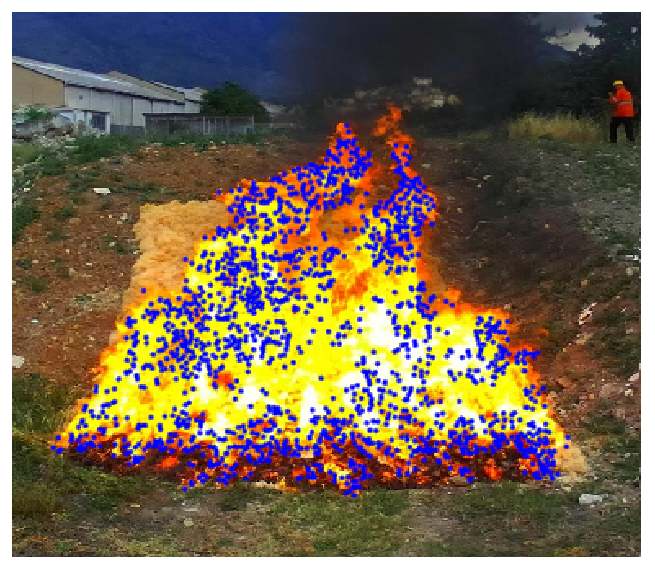
At each image acquisition instant, one visible spectrum image and one LWIR spectrum image are obtained by each Duo Pro R camera. Figure 3 shows an example of fire images obtained simultaneously. A method combining information obtained in the infrared image and in the visible image is used to detect the fire pixels in the visible image.
The MATLAB toolbox code developed by Balcilar [52] with small changes is used to produce superimposed images. The multimodal procedure is performed in two steps. In the first step, the LWIR image is processed with the the Otsu threshold selection method [53] to find the location of the highest intensity pixels corresponding to the fire pixels. Only the pixels situated in the visible image at the same position as those detected in the LWIR image are considered to detect fire pixels.
A fire pixel in the pre-selected area of the visible image is detected as follows: The effectiveness of 11 state-of-the-art fire color segmentation algorithms [22,23,24,25,26,27,28,29,30,31,32] is visually evaluated on the first image of an image sequence associated to a propagating fire with a graphical interface. A previously described method [31] was adapted to use only the second step of this procedure (the first step corresponding to the pixel pre-selection procedure). The procedure that achieved the best pixel detection is then used for all images in the sequence.
2.2.2. Feature Detection, Matching, and Triangulation
Features in the fire areas are detected, such that they can be matched and used in a triangulation method to obtain 3D points. From these 3D data, the geometric characteristics of the fire can be estimated.
Features are detected in the fire areas of images by processing these zones successively with the Harris detection algorithm [54] and the speeded-up robust features (SURF) procedure [55]. The first method is applied with a box filter of pixels. The second one uses six scale levels with the following filter size dimensions: , , , , , and . The points obtained by each procedure are added and duplicate points are deleted.
The zero mean normalized sum of squared differences (ZNSSD) method [56] is used in the feature matching procedure to measure descriptor similarities. Figure 4 shows 1803 matched points obtained from the features detected in the stereoscopic images, with an example shown in Figure 3.
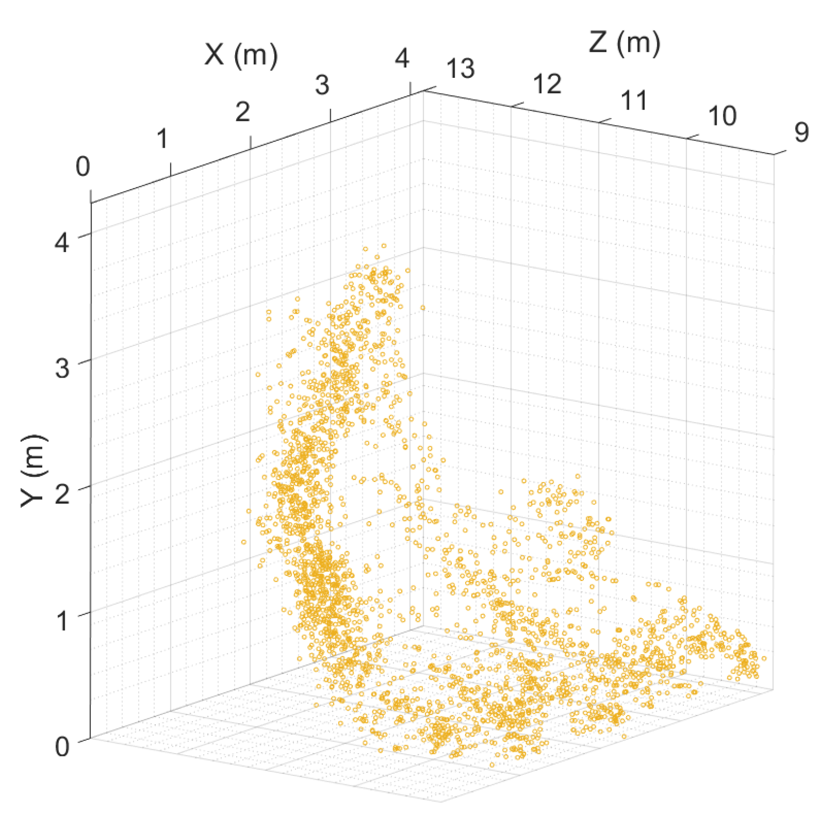
3D fire points are obtained by triangulation, as described in [44], using the coordinates of the matched points and the intrinsic and extrinsic parameters of the stereovision device. Their tridimensional coordinates are given relative to the center of the left camera of the stereovision system. The farthest points from the main cloud are not considered if one of the two conditions presented in Equation (2) is true; in which case, the point is identified as an outlier and is eliminated.
where and are the mean and standard deviation of the distance between this point and its four neighbors, respectively; while and are the mean and standard deviation of the distance between this point and the camera frame origin, respectively.
2.2.3. Fire Local Propagation Plane and Principal Direction Estimation
Fire Local Propagation Plane
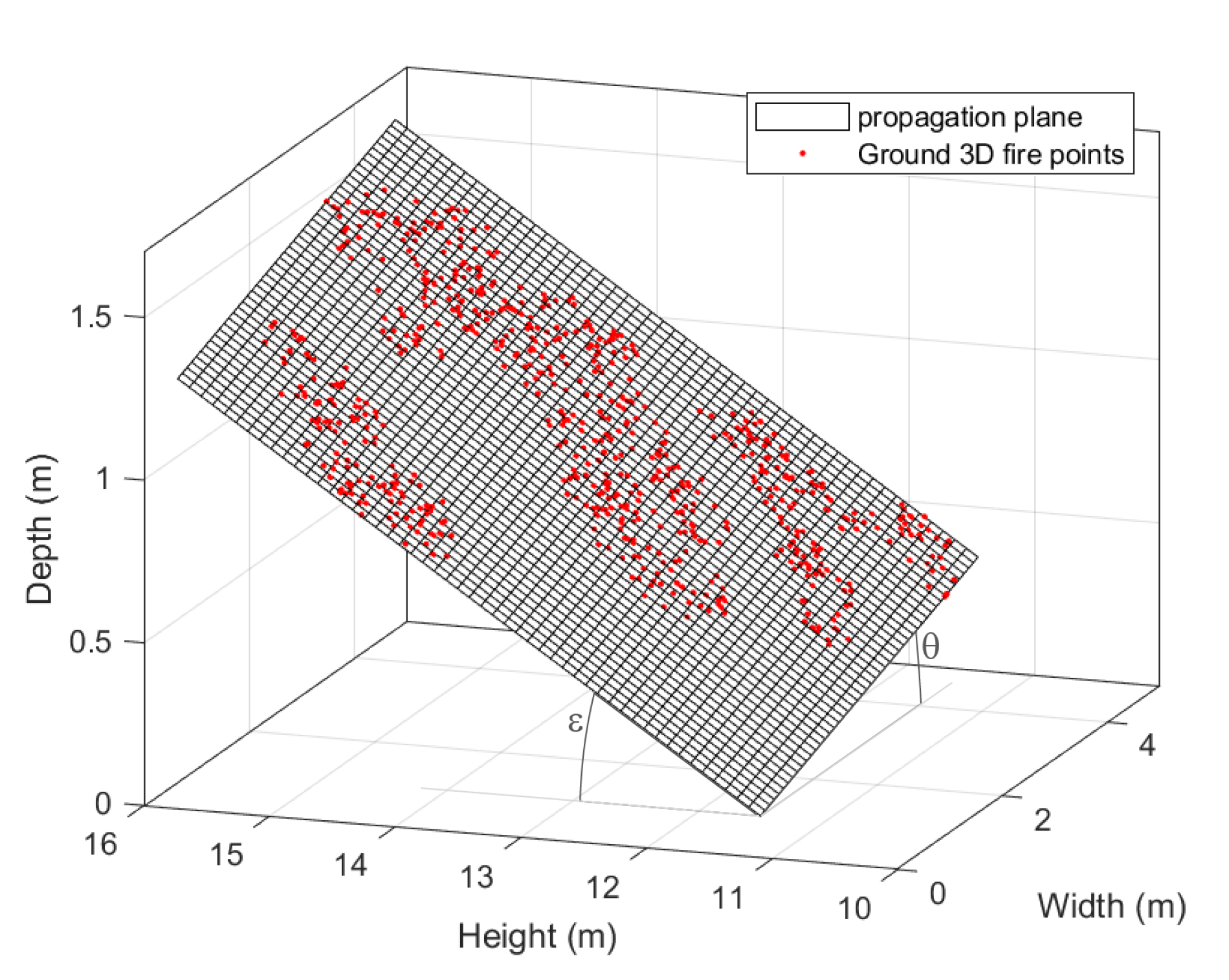
As there is no a priori knowledge about the plane on which the fire spread occurs, the equation of the local propagation plane must be computed in order to estimate information such as the position of the fire on the ground and its height. First, at each image acquisition time, the equation of the local propagation plane is obtained by a least squares method using the lower 3D fire points. Second, the 3D points belonging to planes obtained at successive instants and with slope variations of less than are gathered and used to compute a novel equation of the local plane passing through them. This procedure improves the estimation of the local propagation plane equation. Figure 6 presents the estimated topology of the ground on which the fire shown in Figure 3 propagated. At each instant, the local plane is characterized by its longitudinal angle () and its lateral angle ().
Principal Direction
The principal direction of a fire is needed for the computation of certain characteristics, such as its inclination, width, and length. It is variable during the spread of the fire and depends on the wind and the ground slope. It is given by the vector whose extremities are the barycenters of two successive sets of ground fire points. For this, at time t, the set of points obtained at the time t and those obtained at the instant are used.
2.2.4. 3D Fire Points Transformations
At each instant of image acquisition, the vision system carried by the drone has position and orientation differing from those of the previous moment. As the 3D points obtained by stereovision are expressed in a frame positioned in the vision device (camera frame) and as this frame is moving over time, it is necessary to project all the 3D points into a global reference frame, in order to produce results that show the temporal evolution of the fire geometric characteristics, such as the position of the front line.
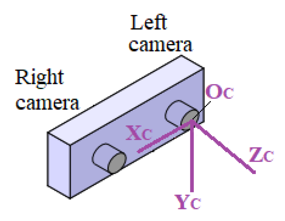
The origin of the camera frame is the optical center of the left visible camera, the x-axis () corresponds to the axis from the left camera towards the right camera, the z-axis () is perpendicular to and directed forward from the cameras, and the y-axis () is the axis perpendicular to the other two axes such that the resulting triad is right-handed, as shown in Figure 7.
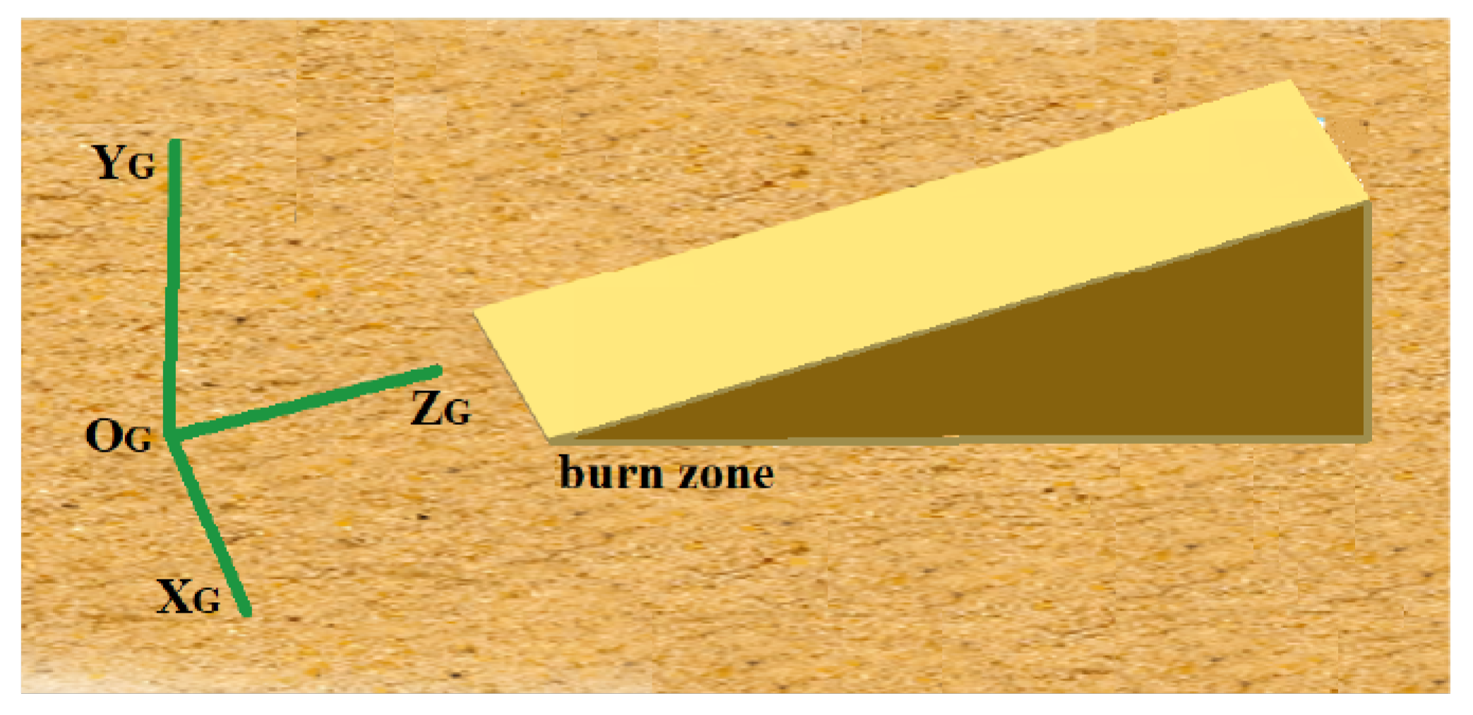
In this work, we chose the GPS data () associated to the first image obtained by the stereovision system before the take-off of the drone as the origin of the global reference frame. The drone was positioned approximately in front of the propagation zone, such that the frame has its x-axis () parallel to the width side of the burn zone. Its z-axis () corresponds to the depth of the burn zone, and the y-axis () is such that the triad is left-handed (i.e., corresponding to the altitude), as shown in Figure 8.
Let , , and be the roll, pitch, and yaw angles estimated by the IMU situated on the vision device when the UAV is flying, respectively. Let , , and be the roll, pitch, and yaw angles estimated by the IMU situated on the vision device before the UAV takes off and associated to the global reference frame, respectively. Let (, and ) be the homogeneous rotation matrices around the x, y, and z axes, respectively. Let T be the translation matrix defined using the coordinates N, E, and U of the position of the vision system in the camera frame—that is,
N, E, and U are computed by applying a transformation on the GPS coordinates of the camera frame in the global coordinate frame.
Let be a homogeneous matrix performing a swap between the y-axis and the z-axis.
The transformation matrix is defined by:
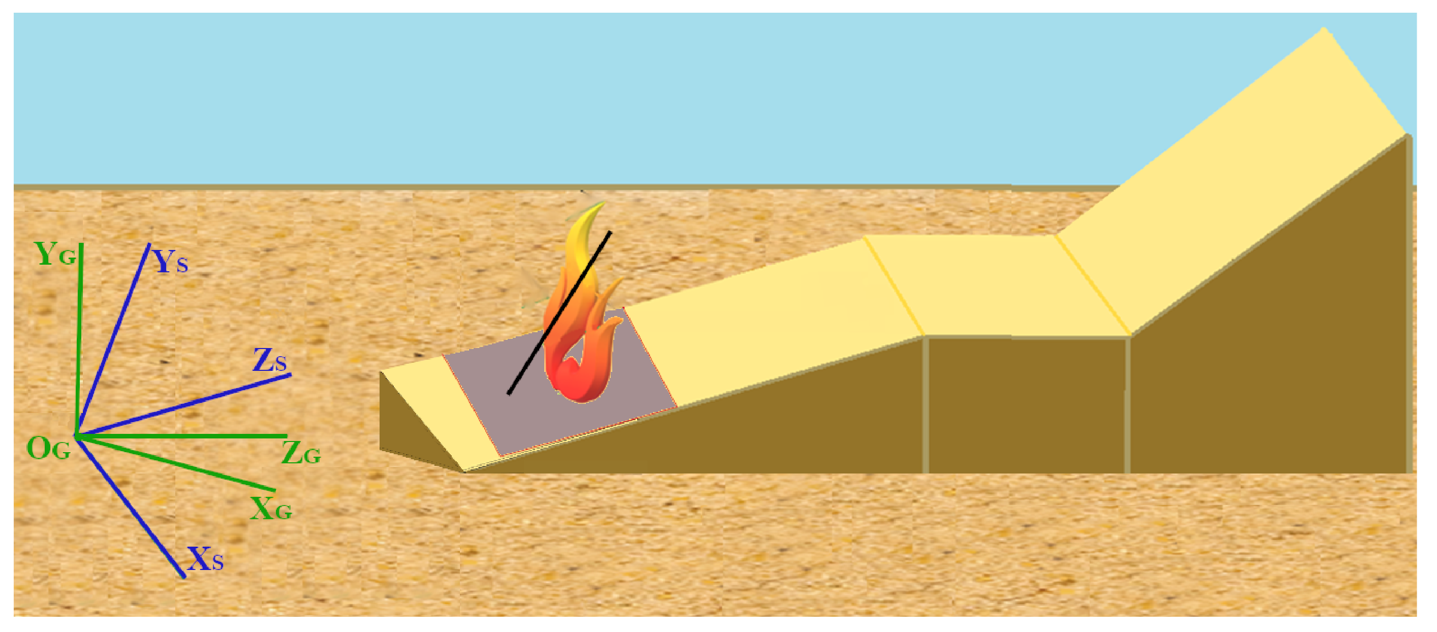
Fire geometric characteristics such as height, length, and inclination angle must be estimated independent of the local propagation plane on which the fire is located. To do this, a transformation function is applied to the 3D fire points, to work as if the slope of the propagation plane was zero. A frame called the “slope frame” is considered; its origin is equal to , its x-axis () is parallel to the ground plane lateral slope, the z-axis () is parallel to the ground plane longitudinal slope, and the y-axis () is parallel to the normal of the ground plane. This frame is considered at each moment of image acquisition (and 3D points calculation), where each local propagation plane (characterized by its average angles and ) imposes an orientation of the S frame, as shown in Figure 9.
The coordinates of the 3D points expressed in the global reference frame are transformed using a matrix . Let and be the longitudinal and lateral angles of the local propagation plane obtained at a given acquisition image instant, respectively. Let and be the homogeneous rotation matrices of the angle around the -axis and of the angle around the axis, respectively. Then, the transformation matrix is defined by:
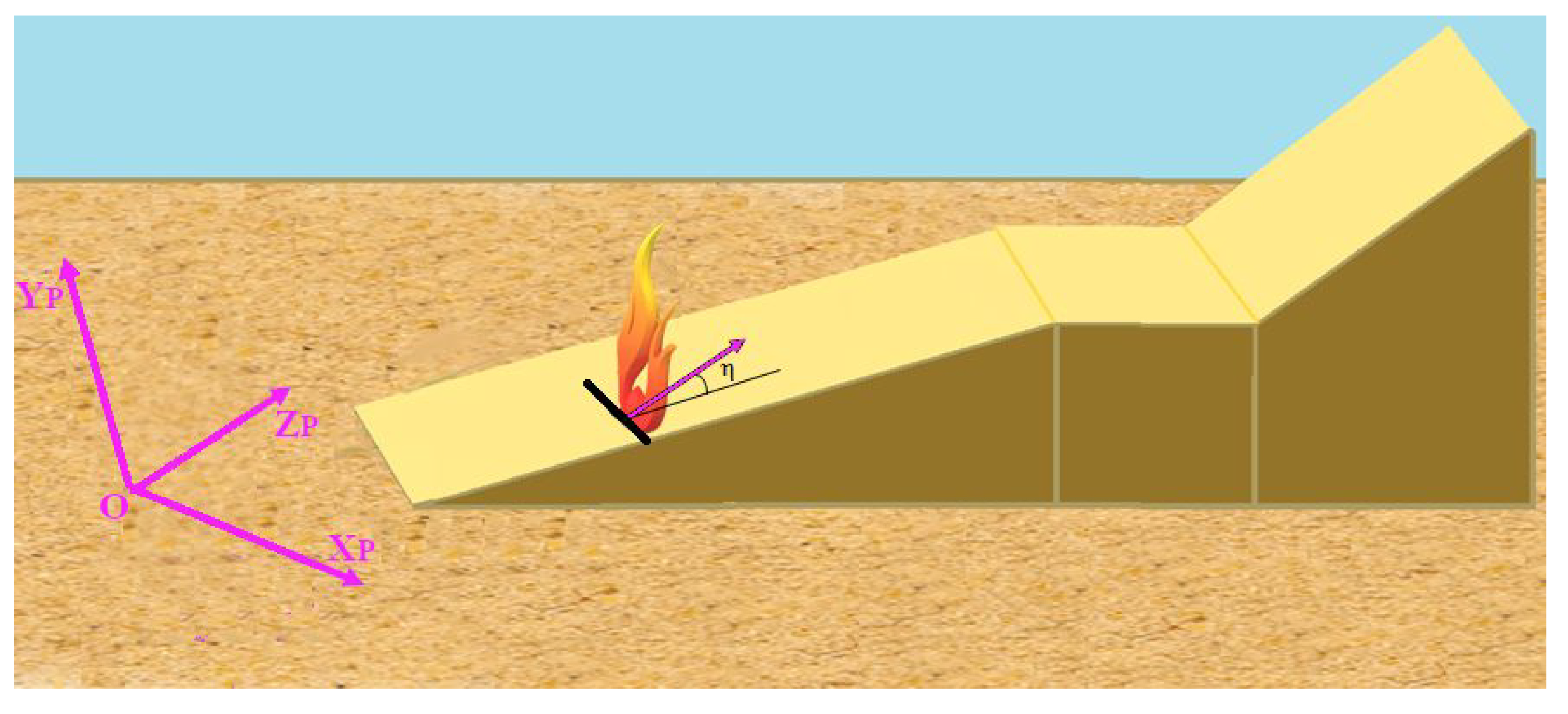
Finally, as the fire may change direction over time, in order to compute geometric characteristics such as width, flame inclination, and length, it is necessary to rotate the 3D points such that the depth axis of the frame used to express them corresponds to the instantaneous direction; the z-axis of the slope frame will be parallel to the instantaneous main direction of the fire at each instant. Let be the angle between the instantaneous fire direction and the z-axis of the slope frame; the 3D fire points are then rotated around the -axis by the angle (Figure 10).
2.2.5. Fire Geometric Characteristics Estimation
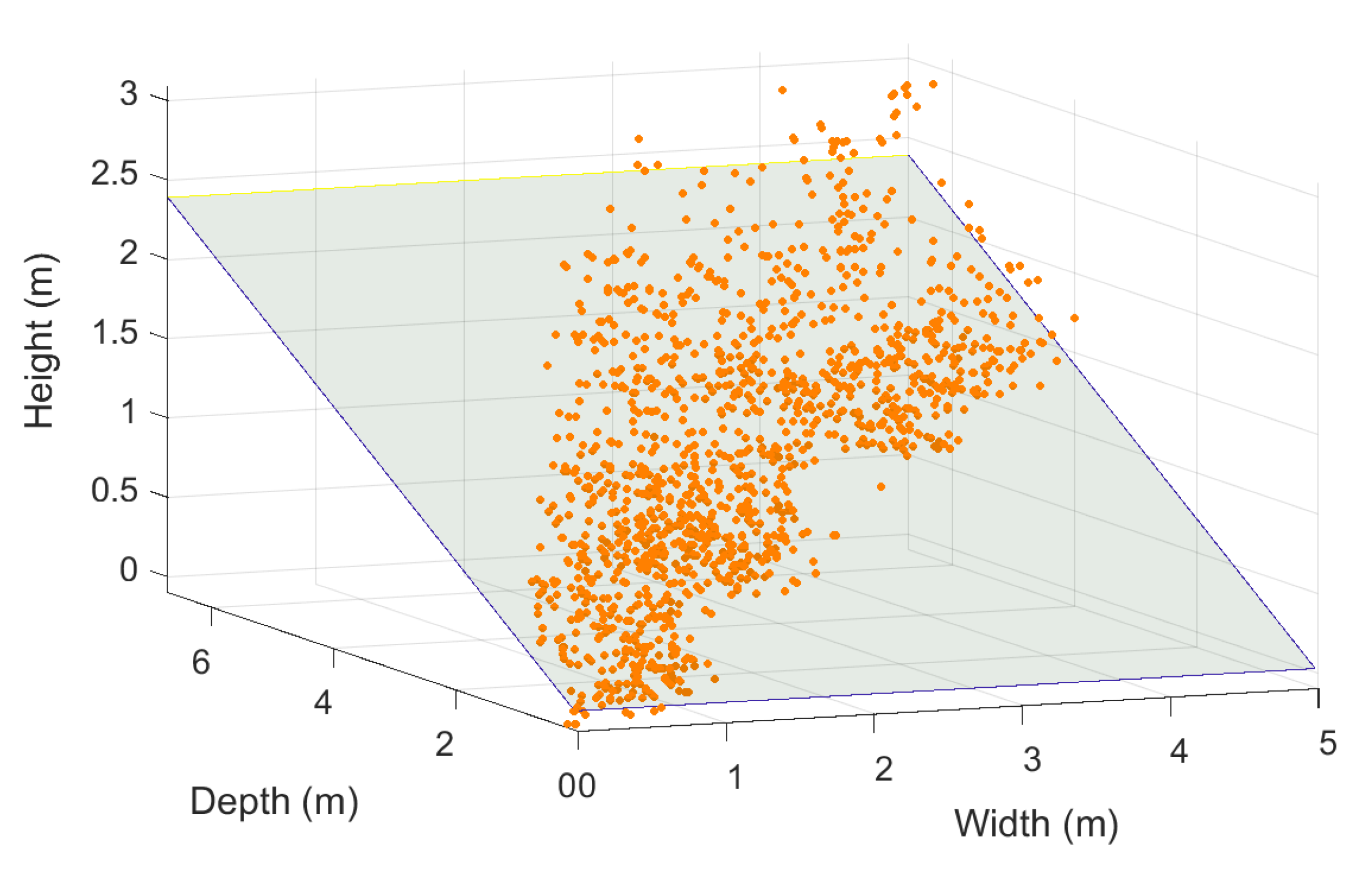
From the transformed 3D fire points, the geometric characteristics of the fire can be estimated. All of the points are used for the 3D reconstruction of the fire and the computation of its surface and view factor. Only the points that are on the ground are considered for the estimation of the front position, base area, width, and depth.
Shape and Volume
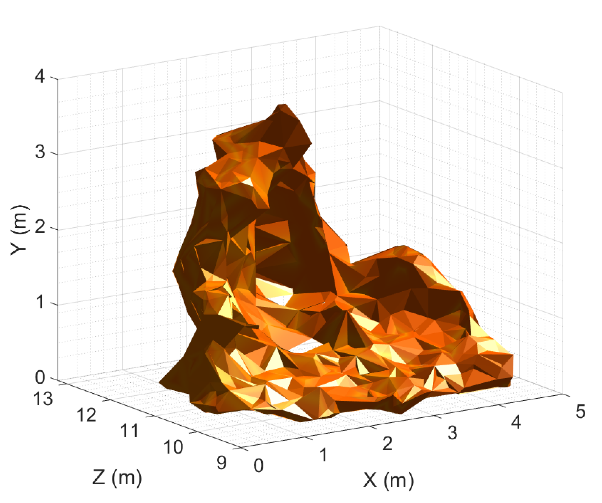
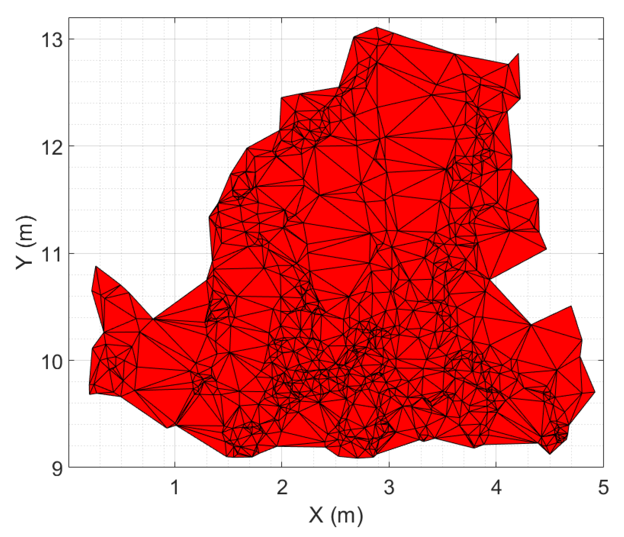
The Delaunay triangulation method is applied to the 3D fire points, which provides a set of tetrahedrons [57]. The 3D fire shape depends on the radius used. Tests were conducted by varying the radius between 0.3 and 0.4 m in steps of 0.01 m; the value that produced the best result was 0.35 m. The tetrahedrons for which the projection of their centers onto the segmented image do not match with fire pixels are eliminated. Figure 11 shows the 3D reconstruction of the fire shown in Figure 3. The sum of the volumes of the selected tetrahedrons is considered to be the volume of the fire.
Surface and View Factor
Considering the set of triangles forming the surface of the fire, it is possible to compute the surface of the fire that produces the heat flux in front of the fire and the fraction of the total energy emitted by the fire surface and received by a target, regardless of its position (also called the view factor).
To compute the fire surface, only the surfaces of the triangles that are not masked by others and which are oriented in the principal direction of the fire are added.
The view factor is estimated by considering all the fire triangles and the 3D coordinates of the target. For this, we used the method described in [58]. The view factor for the radiation between the whole flame surface S and the target area is defined as the fraction of the total energy emitted by all the elementary triangle surfaces and received by . Let be the distance between the target area and the center of the triangle of surface . Let and be the angle between and the normal of the elementary triangle surface and the angle between and the normal of the target surface, respectively. Therefore:
Position, Rate of Spread and Depth
A fire is delimited and localized by its front and back lines. To find them, the points are processed in sectors. For the experiments described in this paper, they were 15 cm wide, but this value can be scaled to the width of the fire, in order to consider different scenarios. In each sector, the most- and least-advanced points are selected. The front (back) line of the fire is obtained using a B-spline interpolation with a polynomial function passing through the most (least) advanced points, as shown in Figure 13.
Over time, the lines move and distort. This can be modeled by considering the velocity of each point of the lines. Researchers working on fire propagation modeling are interested in the rate of spread of characteristic points situated in the center and on the sides of the fire line. This can be estimated by computing the ratio of the distance between two equivalent points on two successive lines divided by the time interval between the two acquisition moments of the images from which the curves were calculated, as previously described in [58]. Considering two successive lines and a given point in the first line, its equivalent point is the intersection point between the normal of the first line passing through the given point and the second line.
The depth of the fire front is estimated by computing the distance between the mean point obtained from the most advanced points and the mean point estimated from the least advanced points.
Combustion Surface
When modeling wildfires, the fuel below a flame contributing to the combustion must be considered; for this purpose, the surface can be approximated by simple forms [59]. From the ground fire points, a polygon is obtained using the method described in [60] (Figure 14). This corresponds to the base of the fire and to the surface of the fuel that is in combustion. Its area is estimated by summing the surface of the triangles contained in the polygon.
Width, Height, Length and Inclination Angle
The fire width, height, length, and inclination angle are computed with 3D points transformed such that the depth axis of the frame used to express them corresponds to the instantaneous direction of the fire.
The fire width is estimated in three steps: First, the two points that have extreme x coordinates among the least-advanced fire ground points are identified. Second, points such that the x coordinate is not more than 15 cm from the latter are used to compute two mean points. Third, the width is computed as the Euclidean distance between the two mean points (Figure 15).
The distance between the base plane and each point of the upper part of the fire corresponds to the height of the point. To produce an average fire height, the mean point of the 3D points situated in the highest 30 cm of the fire is considered.
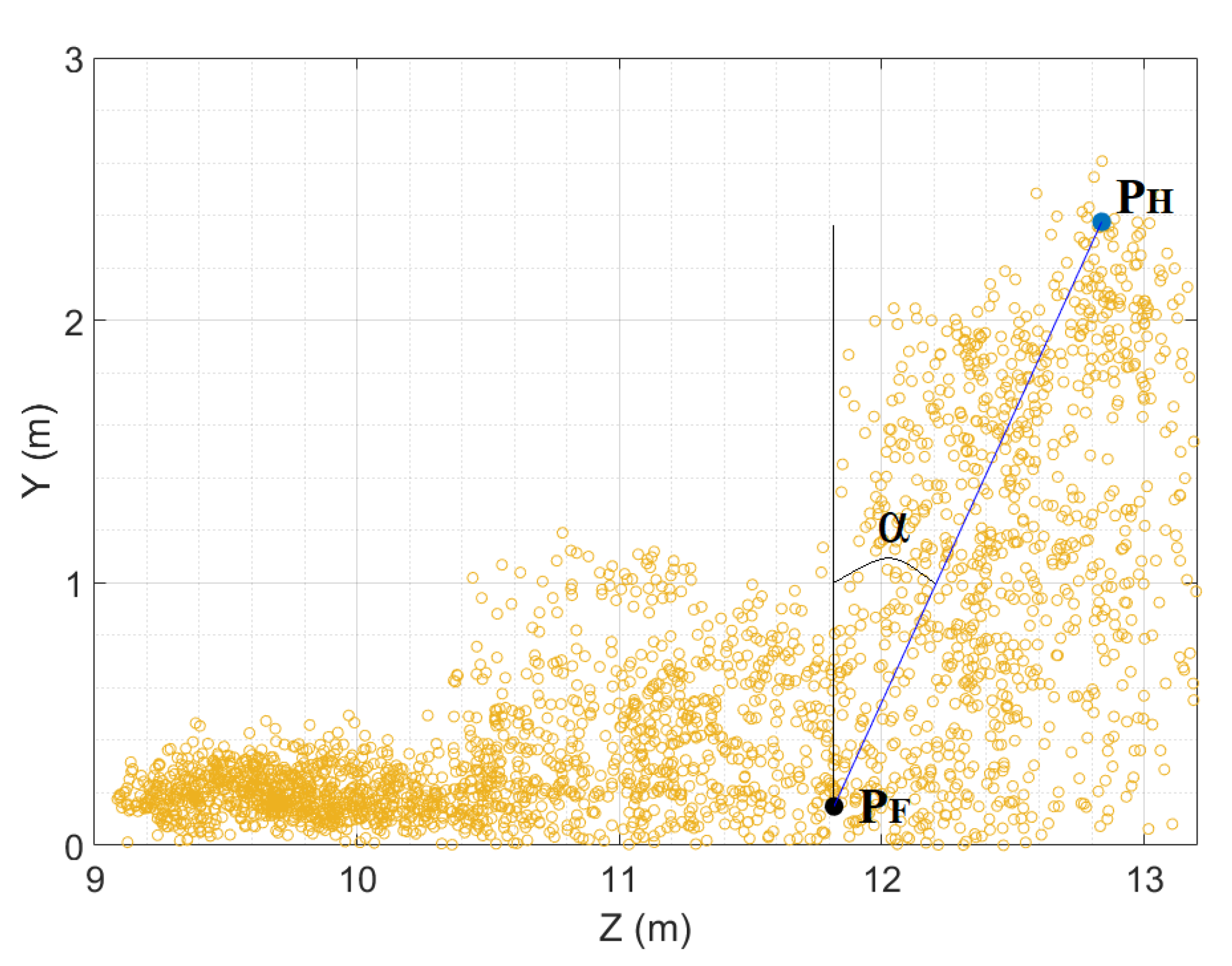
The length of the fire has been defined by researchers working on fire behavior modeling as the distance between the top of the fire front and the most advanced point of the fire base. In this work, the length is calculated as the Euclidean distance between the average point () of the 3D points located within the highest 30 cm of the flame and the average point () of the most advanced ground 3D fire points (Figure 16).
The fire inclination angle is estimated as the angle between the segment and the normal of the fire base plane.
3. Results
Due the unpredictable and non-reproducible behavior of fire, it is difficult to evaluate the uncertainty of the proposed framework.
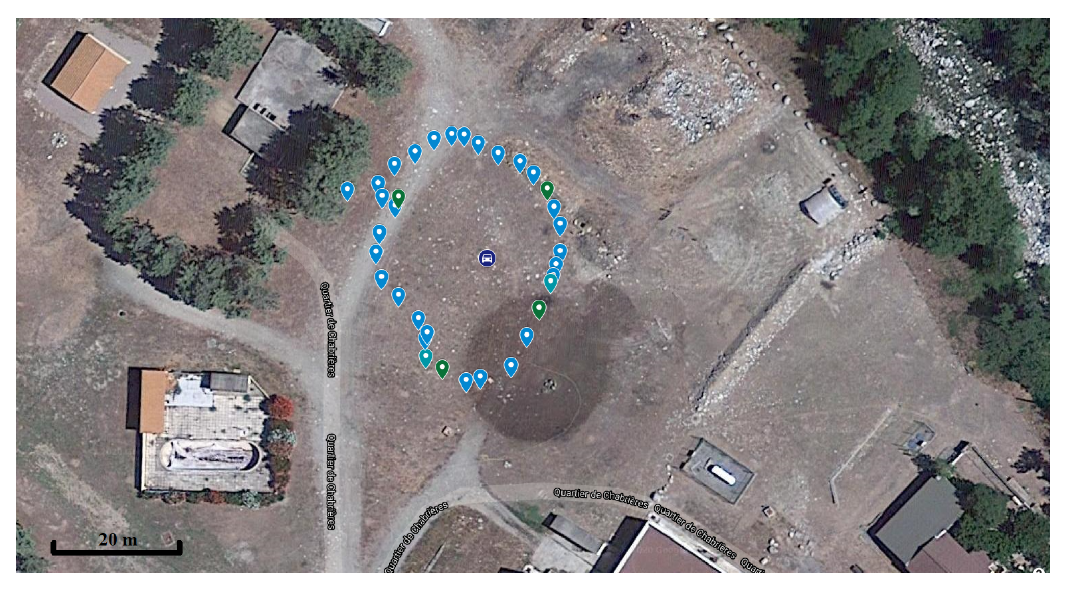
An initial experiment was conducted using a parked car to evaluate the accuracy with which the system evaluates the position of an object and its dimensions. The UAV completed a full turn around the parked car to acquire pictures from each side of the car with a 10–15 m UAV–car distance. The position of the car was measured with a GPS sensor positioned on the roof of the vehicle at the base of the antenna of the car.
Figure 17 shows the GPS position of the drone during the test and the position of the GPS of the car.
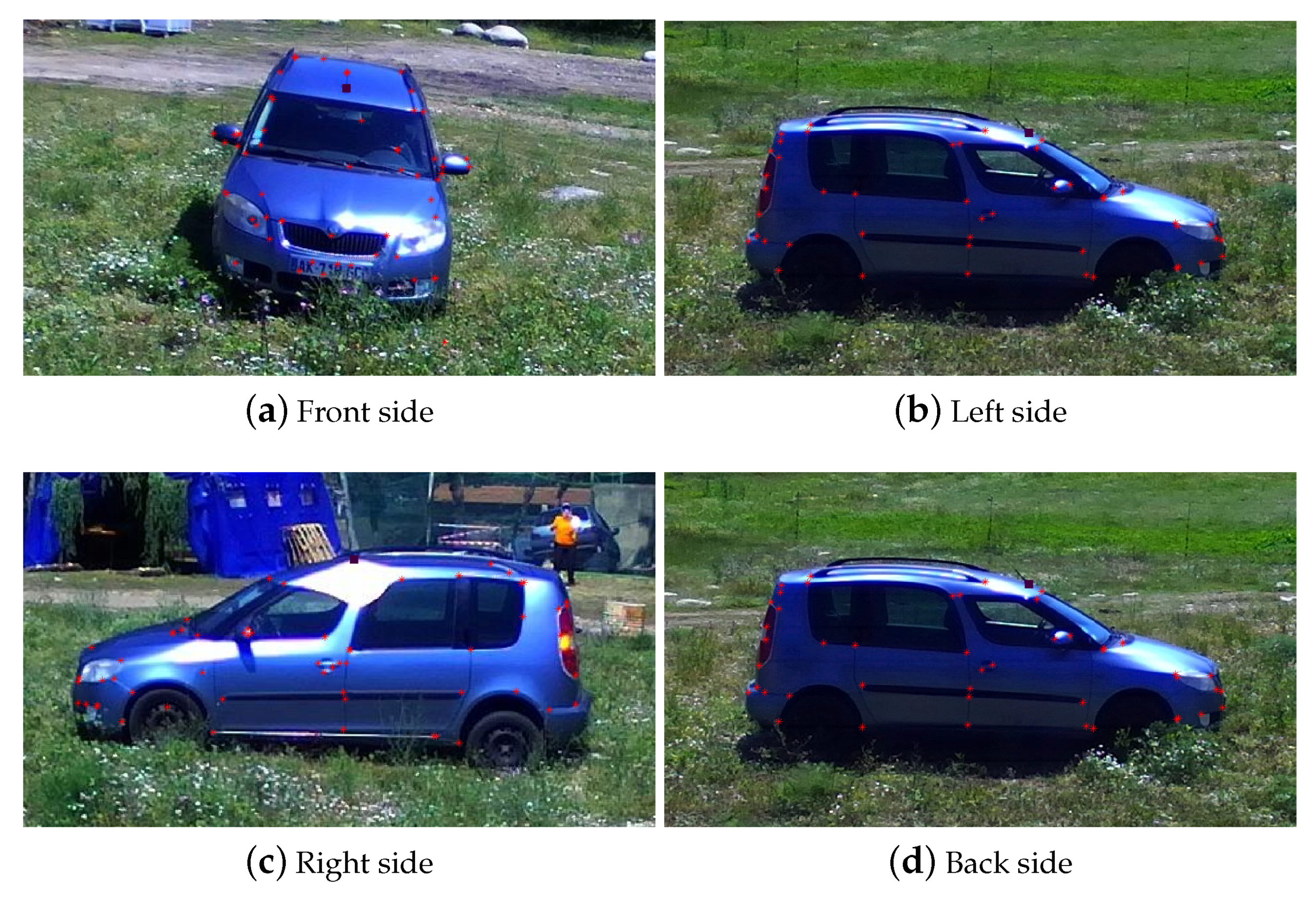
Only visible images were processed and, as the method used for fire pixel detection was not usable, features were selected manually in the images of the four sides of the car. As the goal of this test was to evaluate the efficiency of the framework for estimating the position and the dimensions of an object and not its exact shape, it was not necessary to add the car marks to the homogeneous parts of the car to increase the number of features (Figure 18).
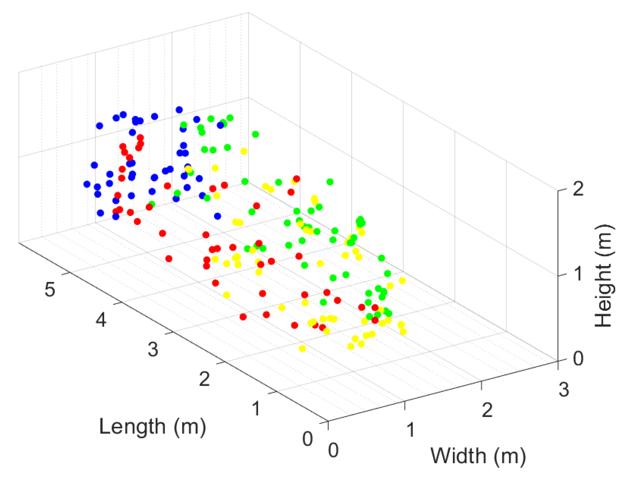
Figure 19 shows the 3D car points obtained separately from the four complementary car views. From each set of points, a surface was computed using the Delaunay method, as shown in Figure 20. Figure 21 presents the complete 3D reconstruction considering all 3D car points in the same set.
We can observe that the overall shape of the vehicle was compatible with the image shown in Figure 18. From the 3D car shape, we estimated the width, height, and length of the car. To estimate the car position, the 3D points of the car antenna were estimated for each car side.
Table 1 presents a comparison between the data estimated by stereovision and the real data (dimensions of the car given by the manufacturer and position of the car obtained with a GPS sensor).
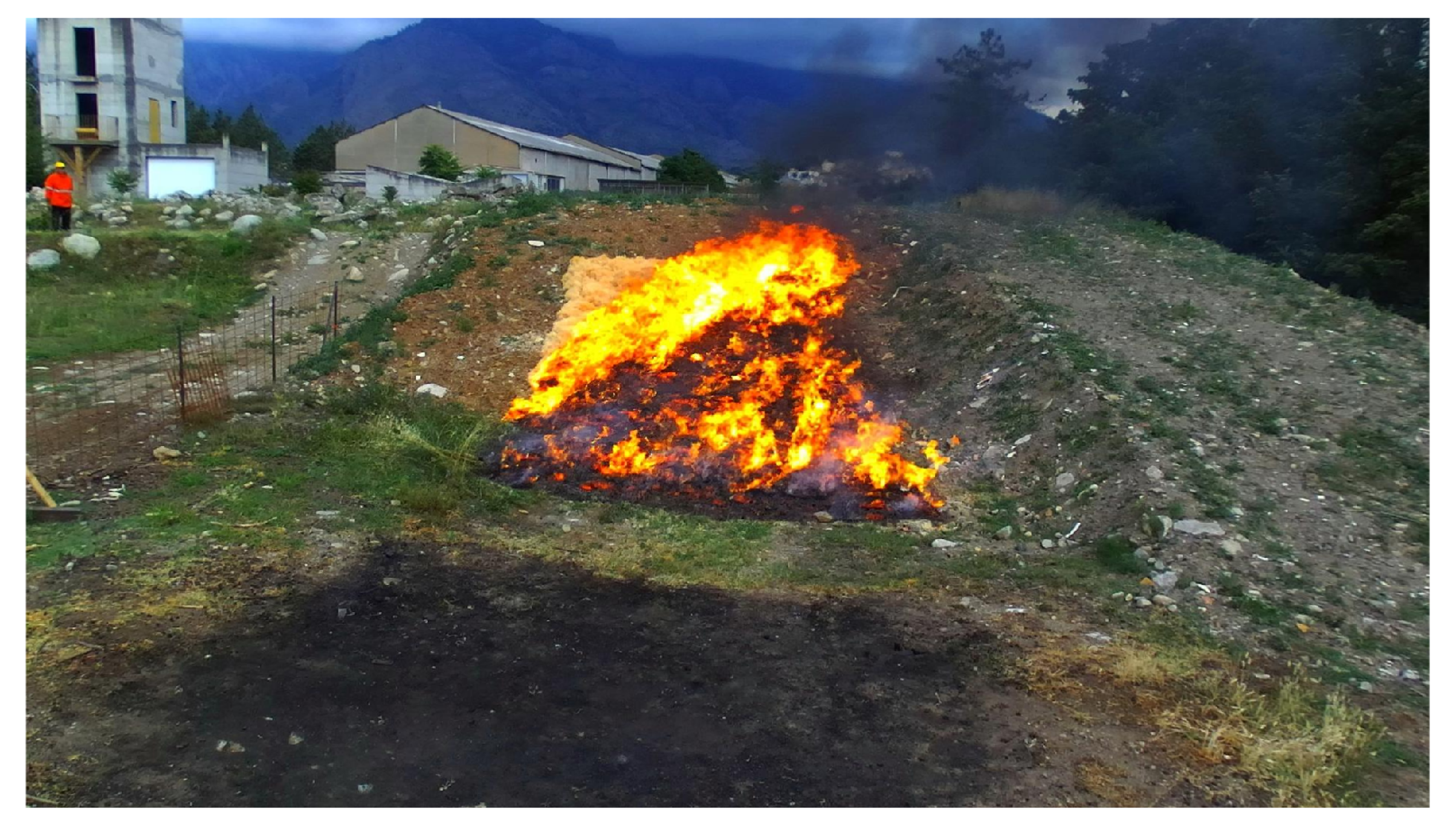
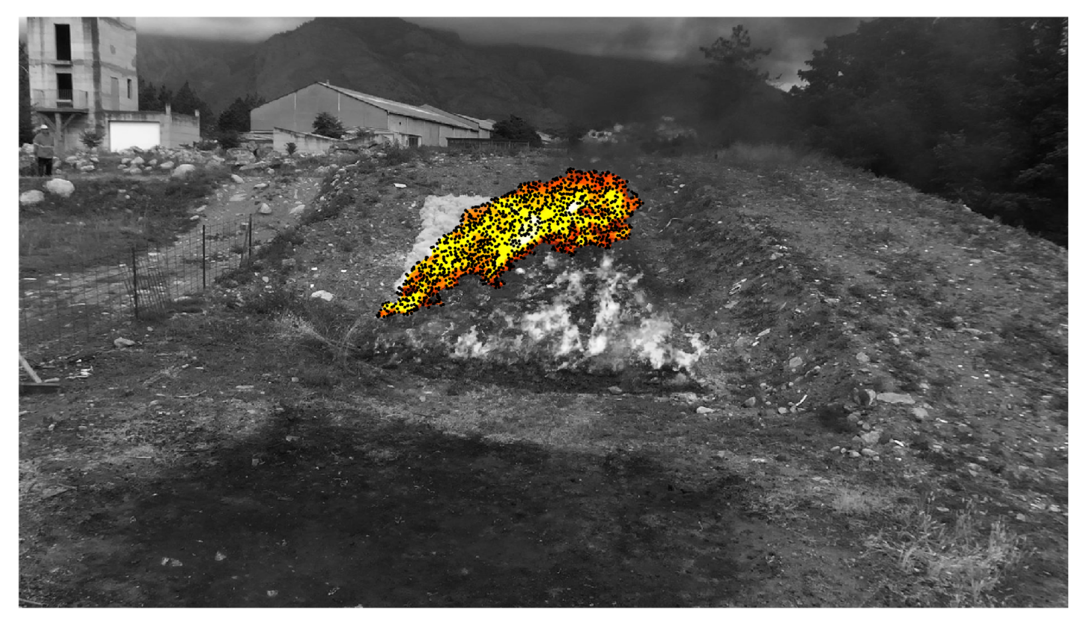
A second experiment was conducted on an outdoor pseudo-static fire. Wood wool was placed on an area of m. The form of the fire changed, but not its position (Figure 22).
At each instant, from the estimated fire points situated on the ground, the front line was obtained. As an example, Figure 23 shows the 3D points computed from the fire image acquired at s and Figure 24 shows the fire front lines estimated at , 96, and 100 s. The form of the lines changed over time but remained in the same position, in keeping with reality.
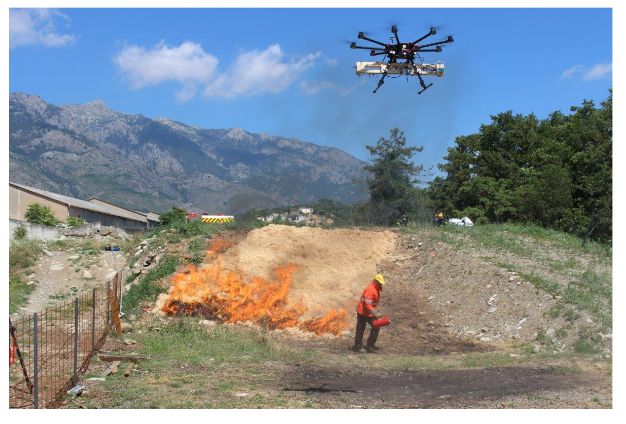
Finally, several tests were conducted outdoors in controlled fire burn areas. All fires were set on a semi-field scale on an area of m consisting of an initial flat zone of 2 m and a second zone with an incline at , which was covered with wood wool (Figure 25).
The drone flew at a height of 10 m, maintaining a distance of 15 m from the fire zone. The inclination of the stereovision system was set to downwards, in order to obtain the best shooting angle at 15 m from the fire. The fire was set along the short side of the rectangle, in order to produce propagation over the entire length of the fuel area along the long side of the rectangle.
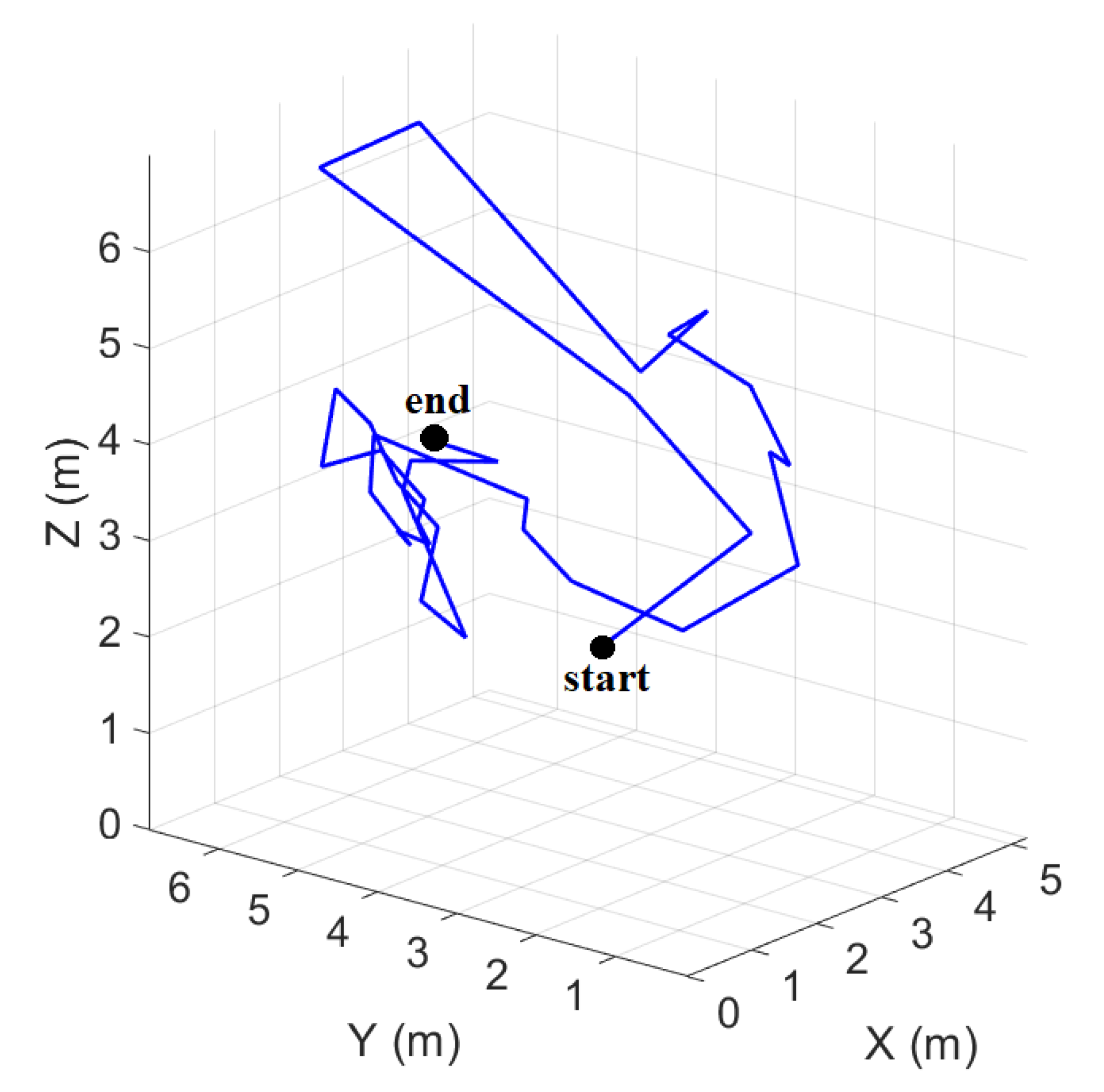
Figure 26 shows the Cartesian positions of the stereovision system during the experiment.
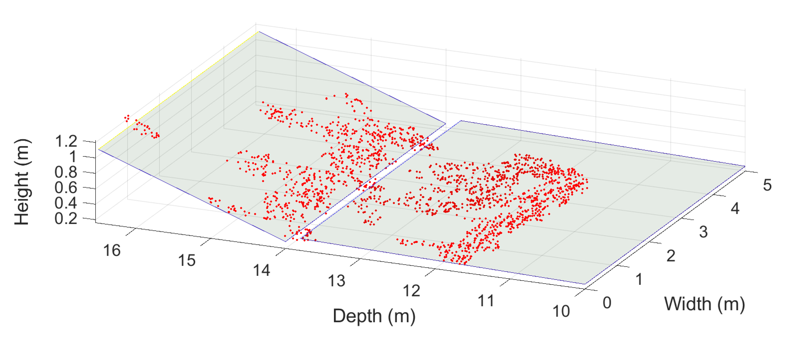
Figure 27 shows the ground 3D fire points obtained for the complete spreading and the estimated propagation plane. The framework modeled the ground in two parts: the first had a longitudinal inclination equal to and the second had a longitudinal inclination equal to . These values were in accordance with the real characteristics of the ground.
Figure 28 shows the fire after a few minutes of propagation. It appears that the fire split into several parts and the frontal first (which is of interest to researchers working on fire behavior modeling) had its ground points at very different depth positions.
Only the frontal part of the fire was considered to produce results. It was identified as the part that corresponded to the biggest part of the fire and had the highest 3D points.
Figure 29 displays the segmented frontal fire area; 1130 matched points were detected in this zone.
Figure 30 shows the 3D points obtained from the matched points presented in Figure 29 and the estimated local propagation plane.
Figure 31 presents the computed 3D reconstruction of the frontal part of the fire. This shape was fully compatible with the image in Figure 28.
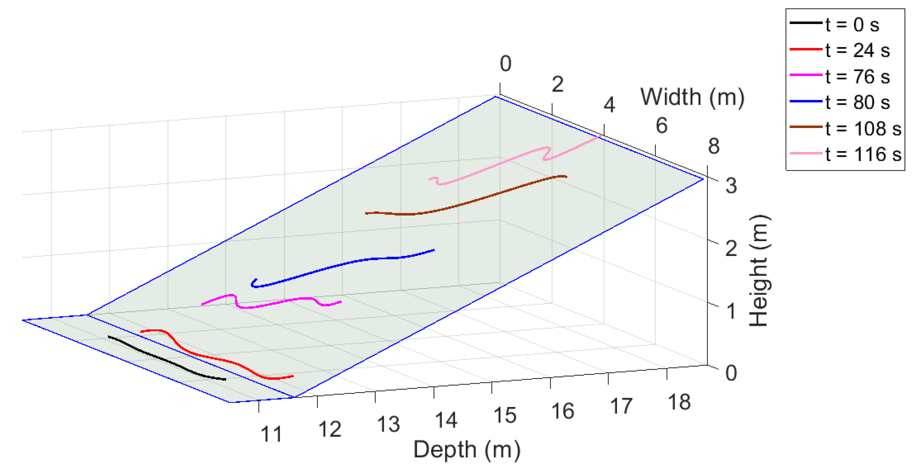
Figure 32 displays the temporal evolution of the fire position, showing the front lines only for certain moments.
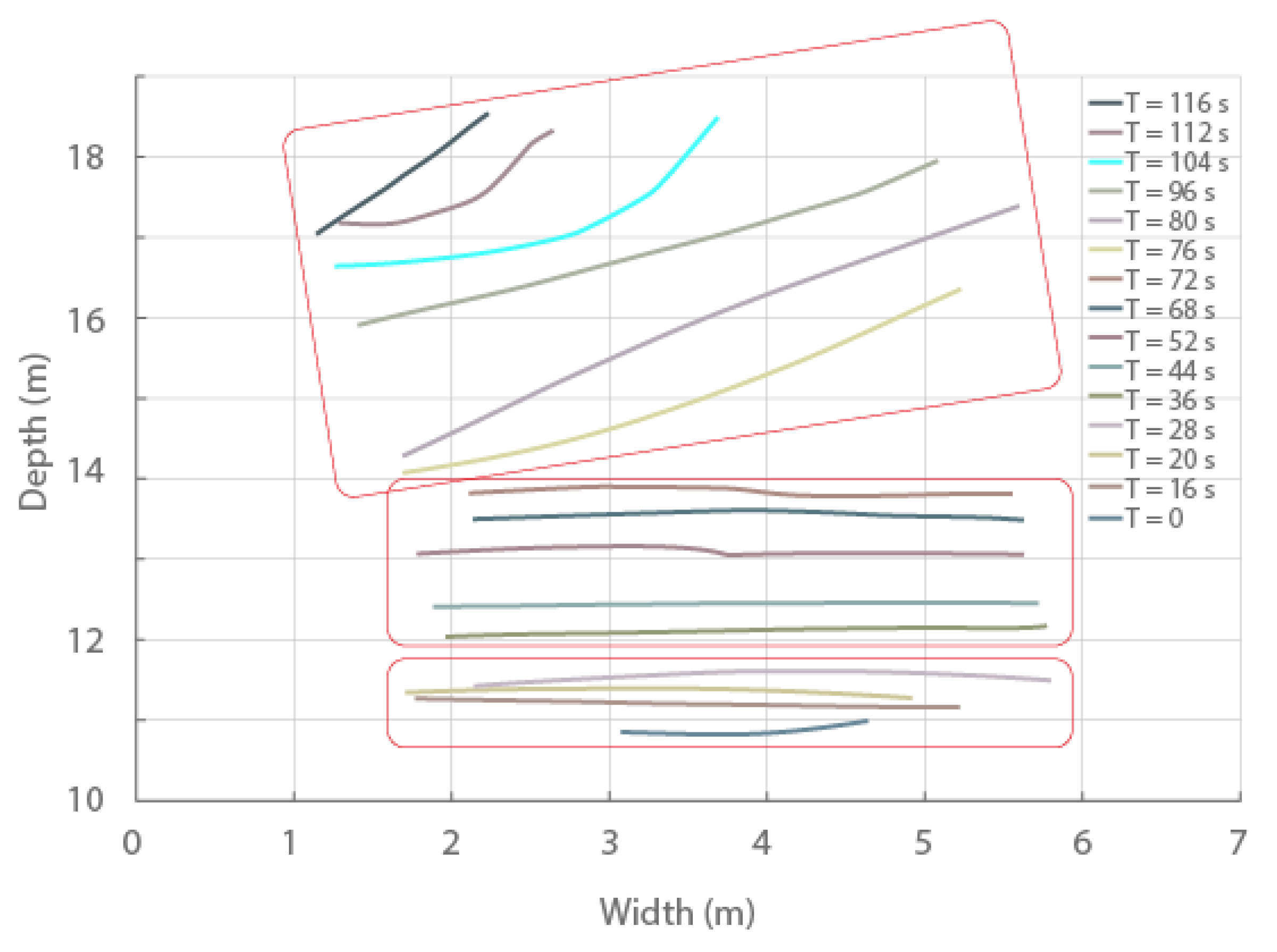
Figure 33 shows the front lines obtained at moments closer together than those considered in Figure 32, with the order of the polynomial function being higher than that used to generate the lines in the previous figure. The lines are clearly smoother than those shown in Figure 32 and were used to identify the fire regimes. A regime is characterized by a constant rate of spread. In this example of fire propagation, three regimes (with relevant lines) were included in the rectangles. These were in accordance with the phenomena occurring over time: first, the fire started on a flat ground with little speed; then, the effect of the ground slope produced fire acceleration; finally, the direction of the wind changed and its intensity increased, resulting in more spaced lines with variation in their normal directions.
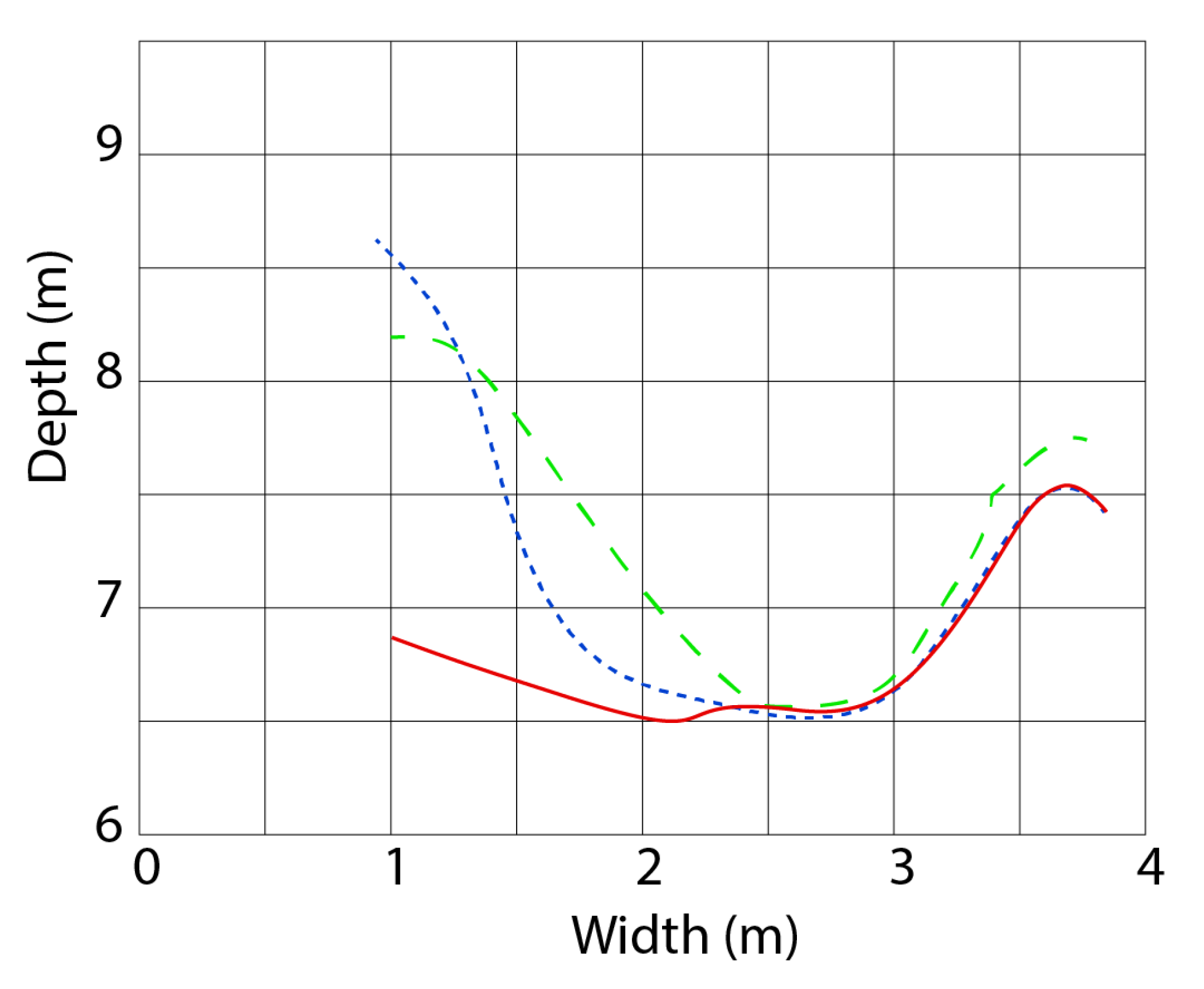
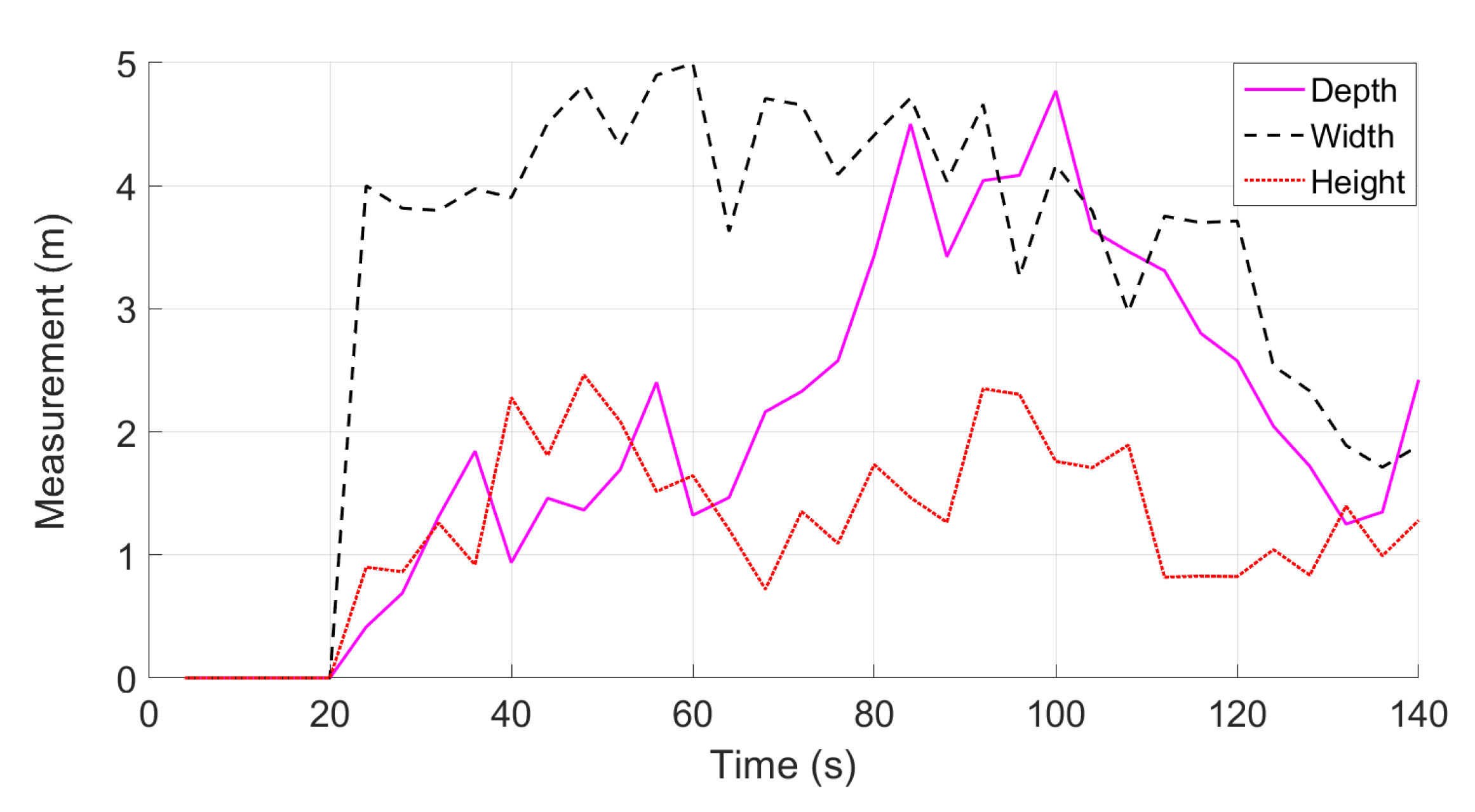
Figure 34 shows the temporal evolution of the fire width, height, and depth. The width varied between 2 and 5 m and was in accordance with the width of the ground and the evolution of the fire trajectory.
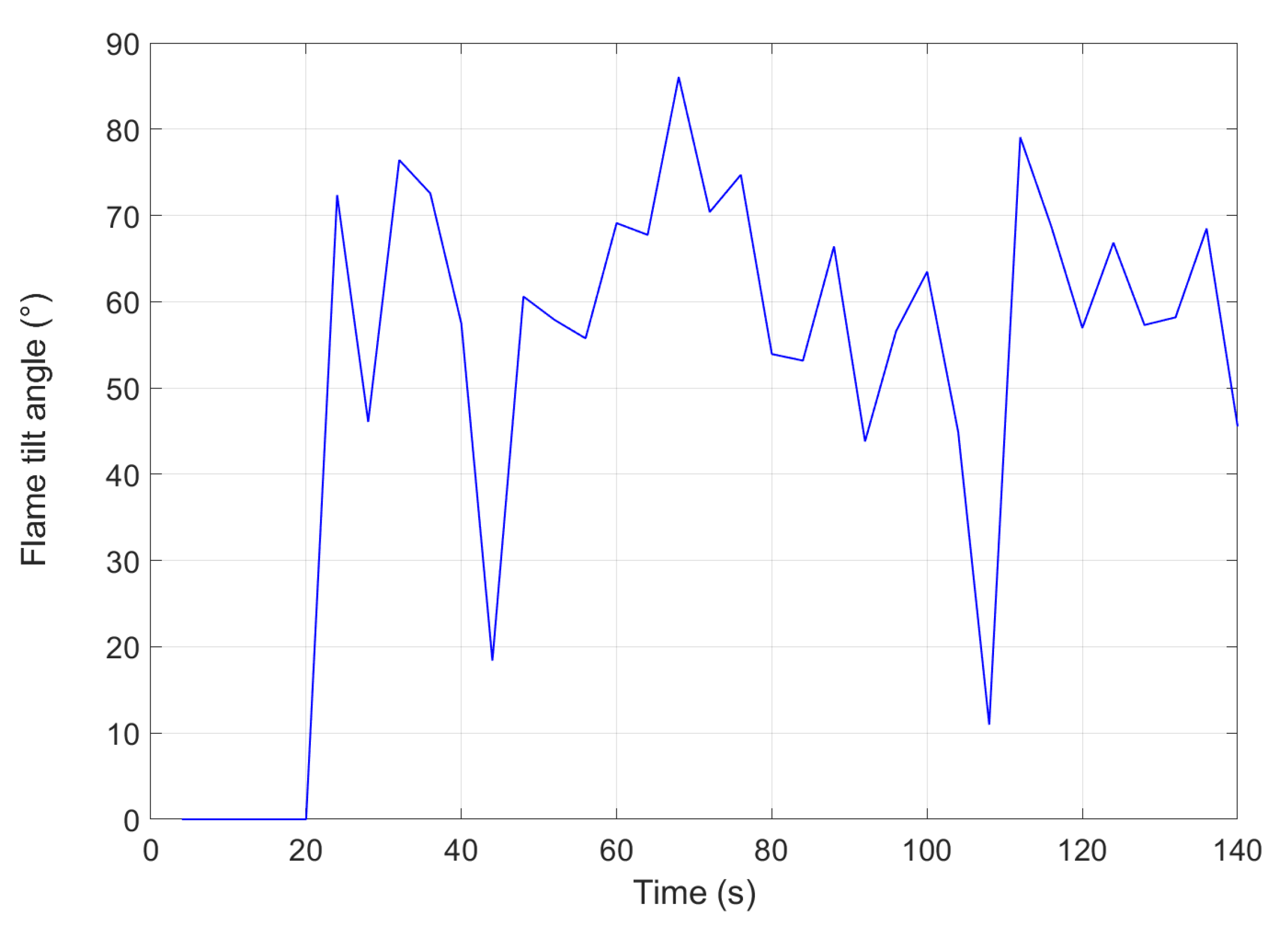
Figure 35 presents the temporal evolution of the maximum flame tilt angle. The curve presents two high tilt angle values, which reflect the strong flame inclinations that were observed during the experiment due to gusts of wind.
The fire considered in this example lasted 120 s and the images obtained in the first 116 s were exploited. The computation was performed using MATLAB 2019b on a computer with an Intel(R) Core(TM) (Intel Corporation, Santa Clara, CA, USA) i7-8650U CPU @ GHz processor and 16 GB of RAM memory. All results were obtained in 46 s (the time taken by the procedure to achieve the best pixel detection method was not counted in this duration).
4. Discussion
Wildfires are a phenomenon whose behavior depends on factors such as the fuel and its load, air humidity, wind, and the slope of the ground. Outdoor experiments cannot possibly reproduce actual fires and, so, obtaining ground truth data is extremely difficult. In this study, two experiments were designed to be as close as possible to ground truth. In the first, we used a parked car with known geometrical characteristics and a UAV flying 10–15 m around it. We found that the estimated dimensions and the position of the car were accurate, demonstrating the validity of the proposed model. The second experiment was conducted using a m area of vegetation, in which the fire did not propagate. The estimated position lines of the fire obtained over time were in line with the experimental situation.
The estimated data obtained during the monitoring of an experimental fire propagated on a m field were consistent with the expectations for this type of propagation; some data correlated to fuel platform dimensions or events such as wind. In future studies, we will use landmarks to provide position and height references for comparison with the measured characteristics.
In the framework presented in this paper, the images were stored on an SD card and processed offline. To use the system onsite in real time, works will be performed to equip the drone with an onboard computer and to reduce the execution time of the programs.
5. Conclusions
In this paper, we proposed a UAV multimodal stereovision framework to measure the geometric characteristics of experimental fires. It is composed of a vision device—integrating two multimodal cameras operating simultaneously in the LWIR and visible spectra—and a UAV. From georeferenced multimodal stereoscopic images, 3D fire points are obtained, from which fire geometric characteristics can be estimated. The framework is able to produce the temporal evolution of the geometric characteristics of a fire propagating over unlimited distance. This satisfies the need for a system that is able to estimate fire geometric characteristics, in order to understand and model wildfire behavior. In future work, the use of this system to monitor controlled burns will be explored.
Author Contributions
Conceptualization, V.C., L.R., and A.P.; methodology, V.C., L.R., and A.P.; validation, V.C. and L.R; formal analysis, V.C. and L.R.; programming, V.C.; investigation, V.C., L.R., and A.P.; resources, L.R., writing—-original draft preparation, V.C. and L.R. All authors have read and agreed to the published version of the manuscript.
Funding
This research was funded by the Corsican Region, the French Ministry of Research and the CNRS under Grant CPER 2014–2020.
Acknowledgments
The authors thank the Company Photos Videos Reporters for its collaboration in the development of the UAV stereovision system and assistance during the execution of experimental tests, and in particular, the support provided by Xavier Carreira. We also thank Elie El Rif, who participated in the development of the vision device during their internship for obtaining a B.Eng. in Telecommunication Engineering at the Holy Spirit University of Kaslik, and to Thierry Marcelli for their help concerning LaTeX and illustration problems. We also thank the anonymous reviewers for their constructive and valuable suggestions on the earlier drafts of this manuscript.
Conflicts of Interest
The authors declare no conflict of interest.
References
- European Science & Technology Advisory Group (E-STAG). Evolving Risk of Wildfires in Europe—The Changing Nature of Wildfire Risk Calls for a Shift in Policy Focus from Suppression to Prevention; United Nations for Disaster Risk Reduction–Regional Office for Europe: Brussels, Belgium, 2020; Available online: https://www.undrr.org/publication/evolving-risk-wildfires-europe-thematic-paper-european-science-technology-advisory (accessed on 29 October 2020).
- European Commission. Forest Fires—Sparking Firesmart Policies in the EU; Research & Publications Office of the European Union: Brussels, Belgium, 2018; Available online: https://ec.europa.eu/info/publications/forest-fires-sparking-firesmart-policies-eu_en (accessed on 29 October 2020).
- Tedim, F.; Leone, V.; Amraoui, M.; Bouillon, C.; Coughlan, M.; Delogu, G.; Fernandes, P.; Ferreira, C.; McCaffrey, S.; McGee, T.; et al. Defining extreme wildfire events: Difficulties, challenges, and impacts. Fire 2018, 1, 9. [Google Scholar] [CrossRef] [Green Version]
- Global Land Cover Change—Wildfires. Available online: http://stateoftheworldsplants.org/2017/report/SOTWP_2017_8_global_land_cover_change_wildfires.pdf (accessed on 25 March 2020).
- Jolly, M.; Cochrane, P.; Freeborn, Z.; Holden, W.; Brown, T.; Williamson, G.; Bowman, D. Climate-induced variations in global wildfire danger from 1979 to 2013. Nat. Commun. 2015, 6, 7537. [Google Scholar] [CrossRef] [PubMed]
- Ganteaume, A.; Jappiot, M. What causes large fires in Southern France. For. Ecol. Manag. 2013, 294, 76–85. [Google Scholar] [CrossRef]
- McArthur, A.G. Weather and Grassland Fire Behaviour; Australian Forest and Timber Bureau Leaflet, Forest Research Institute: Canberra, Australia, 1966. [Google Scholar]
- Rothermel, R.C. A Mathematical Model for Predicting Fire Spread in Wildland Fuels; United States Department of Agriculture: Ogden, UT, USA, 1972. [Google Scholar]
- Morvan, D.; Dupuy, J.L. Modeling the propagation of a wildfire through a Mediterranean shrub using the multiphase formulation. Combust. Flame 2004, 138, 199–210. [Google Scholar] [CrossRef]
- Balbi, J.H.; Rossi, J.L.; Marcelli, T.; Chatelon, F.J. Physical modeling of surface fire under nonparallel wind and slope conditions. Combust. Sci. Technol. 2010, 182, 922–939. [Google Scholar] [CrossRef]
- Balbi, J.H.; Chatelon, F.J.; Rossi, J.L.; Simeoni, A.; Viegas, D.X.; Rossa, C. Modelling of eruptive fire occurrence and behaviour. J. Environ. Sci. Eng. 2014, 3, 115–132. [Google Scholar]
- Sacadura, J. Radiative heat transfer in fire safety science. J. Quant. Spectrosc. Radiat. Transf. 2005, 93, 5–24. [Google Scholar] [CrossRef]
- Rossi, J.L.; Chetehouna, K.; Collin, A.; Moretti, B.; Balbi, J.H. Simplified flame models and prediction of the thermal radiation emitted by a flame front in an outdoor fire. Combust. Sci. Technol. 2010, 182, 1457–1477. [Google Scholar] [CrossRef] [Green Version]
- Chatelon, F.J.; Balbi, J.H.; Morvan, D.; Rossi, J.L.; Marcelli, T. A convective model for laboratory fires with well-ordered vertically-oriented. Fire Saf. J. 2017, 90, 54–61. [Google Scholar] [CrossRef]
- Finney, M.A. FARSITE: Fire Area Simulator-Model Development and Evaluation; Rocky Mountain Research Station: Ogden, UT, USA, 1998. [Google Scholar]
- Linn, R.; Reisner, J.; Colman, J.J.; Winterkamp, J. Studying wildfire behavior using FIRETEC. Int. J. Wildland Fire 2002, 11, 233–246. [Google Scholar] [CrossRef]
- Tymstra, C.; Bryce, R.W.; Wotton, B.M.; Taylor, S.W.; Armitage, O.B. Development and Structure of Prometheus: The Canadian Wildland Fire Growth Simulation Model; Natural Resources Canada: Ottawa, ON, Canada; Canadian Forest Service: Ottawa, ON, Canada; Northern Forestry Centre: Edmonton, AB, Canada, 2009. [Google Scholar]
- Bisgambiglia, P.A.; Rossi, J.L.; Franceschini, R.; Chatelon, F.J.; Bisgambiglia, P.A.; Rossi, L.; Marcelli, T. DIMZAL: A software tool to compute acceptable safety distance. Open J. For. 2017, A, 11–33. [Google Scholar] [CrossRef] [Green Version]
- Rossi, J.L.; Chatelon, F.J.; Marcelli, T. Encyclopedia of Wildfires and Wildland-Urban Interface (WUI) Fires; Springer: Cham, Switzerland, 2018. [Google Scholar] [CrossRef]
- Siegel, R. Howell, J. Thermal Radiation Heat Transfer; Hemisphere Publishing Corporation: Washington, DC, USA, 1994. [Google Scholar] [CrossRef]
- Toulouse, T.; Rossi, L.; Akhloufi, M.; Turgay, C.; Maldague, X. Benchmarking of wildland fire colour segmentation algorithms. IET Image Process. 2015, 9, 1–9. [Google Scholar] [CrossRef] [Green Version]
- Phillips, W., III; Shah, M.; da Vitoria Lobo, N. Flame recognition in video. Pattern Recognit. Lett. 2002, 23, 319–327. [Google Scholar] [CrossRef]
- Chen, T.H.; Wu, P.H.; Chiou, Y.C. An early fire-detection method based on image processing. In Proceedings of the IEEE International Conference on Image Processing (ICIP), Singapore, 24–27 October 2004; pp. 1707–1710. [Google Scholar]
- Horng, W.B.; Peng, J.W.; Chen, C.Y. A new image-based real-time flame detection method using color analysis. In Proceedings of the IEEE Networking, Sensing and Control Proceddings, Tucson, AZ, USA, 19–22 March 2005; pp. 100–105. [Google Scholar]
- Celik, T.; Demirel, H.; Ozkaramanli, H.; Uyguroǧlu, M. Fire detection using statistical color model in video sequences. J. Vis. Commun. Image Represent. 2007, 18, 176–185. [Google Scholar] [CrossRef]
- Ko, B.C.; Cheong, K.H.; Nam, J.Y. Fire detection based on vision sensor and support vector machines. Fire Saf. J. 2009, 44, 322–329. [Google Scholar] [CrossRef]
- Celik, T.; Demirel, H. Fire detection in video sequences using a generic color model. Fire Saf. J. 2009, 44, 147–158. [Google Scholar] [CrossRef]
- Celik, T. Fast and efficient method for fire detection using image processing. ETRI J. 2010, 32, 881–890. [Google Scholar] [CrossRef] [Green Version]
- Chitade, A.Z.; Katiyar, S. Colour based image segmentation using k-means clustering. Int. J. Eng. Sci. Technol. 2010, 2, 5319–5325. [Google Scholar]
- Collumeau, J.F.; Laurent, H.; Hafiane, A.; Chetehouna, K. Fire scene segmentations for forest fire characterization: A comparative study. In Proceedings of the 18th IEEE International Conference on Image Processing (ICIP), Brussels, Belgium, 11–14 September 2011; pp. 2973–2976. [Google Scholar]
- Rossi, L.; Akhloufi, M.; Tison, Y. On the use of stereovision to develop a novel instrumentation system to extract geometric fire fronts characteristics. Fire Saf. J. 2011, 46, 9–20. [Google Scholar] [CrossRef]
- Rudz, S.; Chetehouna, K.; Hafiane, A.; Laurent, H.; Séro-Guillaume, O. Investigation of a novel image segmentation method dedicated to forest fire applications. Meas. Sci. Technol. 2013, 24, 075403. [Google Scholar] [CrossRef]
- Toulouse, T.; Rossi, L.; Celik, T.; Campana, A.; Akhloufi, M. Computer vision for wildfire research: An evolving image dataset for processing and analysis. Fire Saf. J. 2017, 92, 188–194. [Google Scholar] [CrossRef] [Green Version]
- Gouverneur, B.; Verstockt, S.; Pauwels, E.; Han, J.; de Zeeuw, P.M.; Vermeiren, J. Archeological treasures protection based on early forest wildfire multi-band imaging detection system. In Proceedings of the Electro-Optical and Infrared Systems: Technology and Applications IX, Edinburgh, UK, 24 October 2012; p. 85410J. [Google Scholar] [CrossRef]
- Billaud, Y.; Boulet, P.; Pizzo, Y.; Parent, G.; Acem, Z.; Kaiss, A.; Collin, A.; Porterie, B. Determination of woody fuel flame properties by means of emission spectroscopy using a genetic algorithm. Combust. Sci. Technol. 2013, 185, 579–599. [Google Scholar] [CrossRef]
- Verstockt, S.; Vanoosthuyse, A.; Van Hoecke, S.; Lambert, P.; Van de Walle, R. Multi-sensor fire detection by fusing visual and non-visual flame features. In Proceedings of the International Conference on Image and Signal Processing, Quebec, QC, Canada, 30 June–2 July 2010; pp. 333–341. [Google Scholar] [CrossRef] [Green Version]
- Verstockt, S.; Van Hoecke, S.; Beji, T.; Merci, B.; Gouverneur, B.; Cetin, A.; De Potter, P.; Van de Walle, R. A multimodal video analysis approach for car park fire detection. Fire Saf. J. 2013, 57, 9–20. [Google Scholar] [CrossRef]
- Clements, H.B. Measuring fire behavior with photography. Photogram. Eng. Remote Sens. 1983, 49, 213–219. [Google Scholar]
- Pastor, E.; Águeda, A.; Andrade-Cetto, J.; Muñoz, M.; Pérez, Y.; Planas, E. Computing the rate of spread of linear flame fronts by thermal image processing. Fire Saf. J. 2006, 41, 569–579. [Google Scholar] [CrossRef] [Green Version]
- De Dios, J.R.M.; André, J.C.; Gonçalves, J.C.; Arrue, B.C.; Ollero, A.; Viegas, D. Laboratory fire spread analysis using visual and infrared images. Int. J. Wildland Fire 2006, 15, 179–186. [Google Scholar] [CrossRef]
- Verstockt, S.; Van Hoecke, S.; Tilley, N.; Merci, B.; Lambert, P.; Hollemeersch, C.; Van de Walle, R. FireCube: A multi-view localization framework for 3D fire analysis. Fire Saf. J. 2011, 46, 262–275. [Google Scholar] [CrossRef]
- Martinez-de Dios, J.R.; Arrue, B.C.; Ollero, A.; Merino, L.; Gómez-Rodríguez, F. Computer vision techniques for forest fire perception. Image Vis. Comput. 2008, 26, 550–562. [Google Scholar] [CrossRef]
- Martínez-de Dios, J.R.; Merino, L.; Caballero, F.; Ollero, A. Automatic forest-fire measuring using ground stations and unmanned aerial systems. Sensors 2011, 11, 6328–6353. [Google Scholar] [CrossRef] [Green Version]
- Hartley, R.; Zisserman, A. Multiple View Geometry in Computer Vision; Cambridge University Press: Cambridge, UK, 2003. [Google Scholar]
- Ng, W.B.; Zhang, Y. Stereoscopic imaging and reconstruction of the 3D geometry of flame surfaces. Exp. Fluids 2003, 34, 484–493. [Google Scholar] [CrossRef]
- Rossi, L.; Molinier, T.; Akhloufi, M.; Tison, Y.; Pieri, A. Estimating the surface and the volume of laboratory-scale wildfire fuel using computer vision. IET Image Process. 2013, 6, 1031–1040. [Google Scholar] [CrossRef]
- Toulouse, T.; Rossi, L.; Akhloufi, M.; Pieri, A.; Maldague, X. A multimodal 3D framework for fire characteristics estimation. Meas. Sci. Technol. 2018, 29, 025404. [Google Scholar] [CrossRef]
- Trucco, E.; Verri, A. Introductory Techniques for 3-D Computer Vision; Prentice Hall: Englewood Cliffs, NJ, USA, 1998. [Google Scholar]
- Ciullo, V.; Rossi, L.; Toulouse, T.; Pieri, A. Fire geometrical characteristics estimation using a visible stereovision system carried by unmanned aerial vehicle. In Proceedings of the 15th International Conference on Control, Automation, Robotics and Vision (ICARCV), Singapore, 18–21 November 2018; pp. 1216–1221. [Google Scholar] [CrossRef]
- FLIR Duo Pro R Specifications. Available online: Https://www.flir.com/products/duo-pro-r/ (accessed on 14 October 2020).
- Camera Calibration Toolbox for Matlab. Available online: Http://www.vision.caltech.edu/bouguetj/calib_doc/ (accessed on 14 October 2020).
- Balcilar, M. Stereo Camera Calibration under Different Resolution. 2019. Available online: https://github.com/balcilar/Calibration-Under_Different-Resolution (accessed on 14 October 2020).
- Otsu, N. A threshold selection method from gray-level histograms. IEEE Trans. Syst. Man Cybern. 1979, 9, 62–66. [Google Scholar] [CrossRef] [Green Version]
- Harris, C.G.; Stephens, M. A combined corner and edge detector. In Proceedings of the Alvey Vision Conference, Manchester, UK, 31 August–2 September 1988; pp. 147–151. [Google Scholar]
- Bay, H.; Tuytelaars, T.; Van Gool, L. Surf: Speeded up Robust Features; Springer: Berlin/Heidelberg, Germany, 2006. [Google Scholar]
- Brown, M.; Szeliski, R.; Winder, S. Multi-Image Matching Using Multi-Scale Oriented Patches. In Proceedings of the IEEE Computer Vision and Pattern Recognition Conference (CVPR), San Diego, CA, USA, 20–25 June 2005; pp. 510–517. [Google Scholar]
- Delaunay, B. Sur la sphere vide. Izv. Akad. Nauk SSSR Otd. Mat. I Estestv. Nauk 1934, 7, 793–800. [Google Scholar]
- Rossi, L.; Molinier, T.; Pieri, A.; Tison, Y.; Bosseur, F. Measurement of the geometrical characteristics of a fire front by stereovision techniques on field experiments. Meas. Sci. Technol. 2011, 22, 125504. [Google Scholar] [CrossRef]
- Moretti, B. Modélisation du Comportement des Feux de Forêt pour des Outils d’aide à la Décision. Ph.D. Thesis, University of Corsica, Corte, France, 2015. [Google Scholar]
- Edelsbrunner, H.; Kirkpatrick, D.; Seidel, R. On the shape of a set of points in the plane. IEEE Trans. Inf. Theory 1983, 29, 551–559. [Google Scholar] [CrossRef] [Green Version]
Figure 1.
Stereovision system with two multimodal cameras fixed on an M600 DJI unmanned aerial vehicle (UAV).
Figure 1.
Stereovision system with two multimodal cameras fixed on an M600 DJI unmanned aerial vehicle (UAV).

Figure 2.
Diagram of the proposed methodology.

Figure 3.
Example of images acquired simultaneously in the (a) visible and (b) long wavelength infrared spectra.
Figure 3.
Example of images acquired simultaneously in the (a) visible and (b) long wavelength infrared spectra.

Figure 4.
Matched points obtained from the features in Figure 3.
Figure 4.
Matched points obtained from the features in Figure 3.

Figure 5.
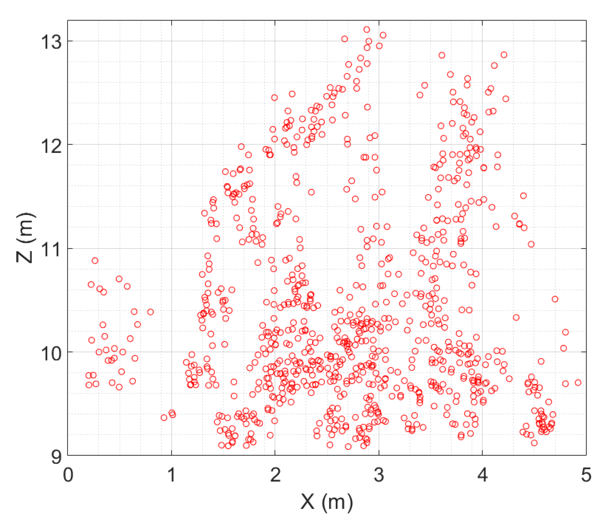
3D fire points.

Figure 6.
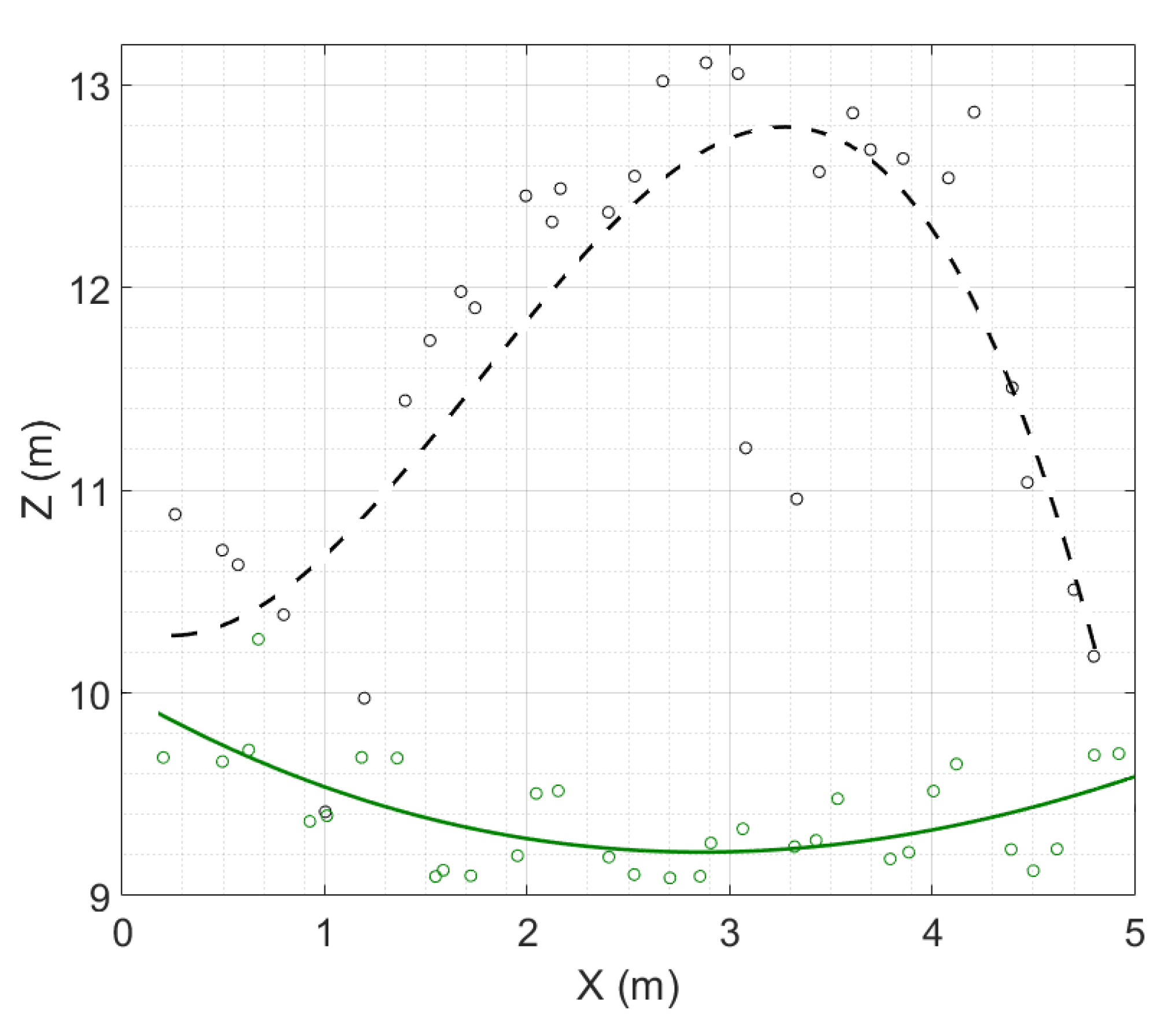
Example of the propagation plane obtained from the lower 3D points of a spreading fire.

Figure 7.
Position and orientation of the camera frame.

Figure 8.
Position and orientation of the global frame.

Figure 9.
Slope frame (blue) and global frame (green). The black line represents the normal of the local.
Figure 9.
Slope frame (blue) and global frame (green). The black line represents the normal of the local.

Figure 10.
Depth axis of the global frame corresponding to the instantaneous fire direction. The pink vector represents the instantaneous direction of the fire.
Figure 10.
Depth axis of the global frame corresponding to the instantaneous fire direction. The pink vector represents the instantaneous direction of the fire.

Figure 11.
3D reconstruction with Delaunay triangulation of the fire shown in Figure 3.
Figure 11.
3D reconstruction with Delaunay triangulation of the fire shown in Figure 3.

Figure 12.
Ground fire 3D points.

Figure 13.
Front line (dashed black line) and back line (solid green line) of the the fire presented in Figure 3.
Figure 13.
Front line (dashed black line) and back line (solid green line) of the the fire presented in Figure 3.

Figure 14.
Fire base combustion of the fire presented in Figure 3.
Figure 14.
Fire base combustion of the fire presented in Figure 3.

Figure 15.
Fire width: distance between the mean points (filled blue circles) of the two sets of points (blue empty circles) having extreme x coordinates among the least advanced fire ground points (blue empty circles).
Figure 15.
Fire width: distance between the mean points (filled blue circles) of the two sets of points (blue empty circles) having extreme x coordinates among the least advanced fire ground points (blue empty circles).

Figure 16.
Length and inclination angle () of the fire presented in Figure 3.
Figure 16.
Length and inclination angle () of the fire presented in Figure 3.

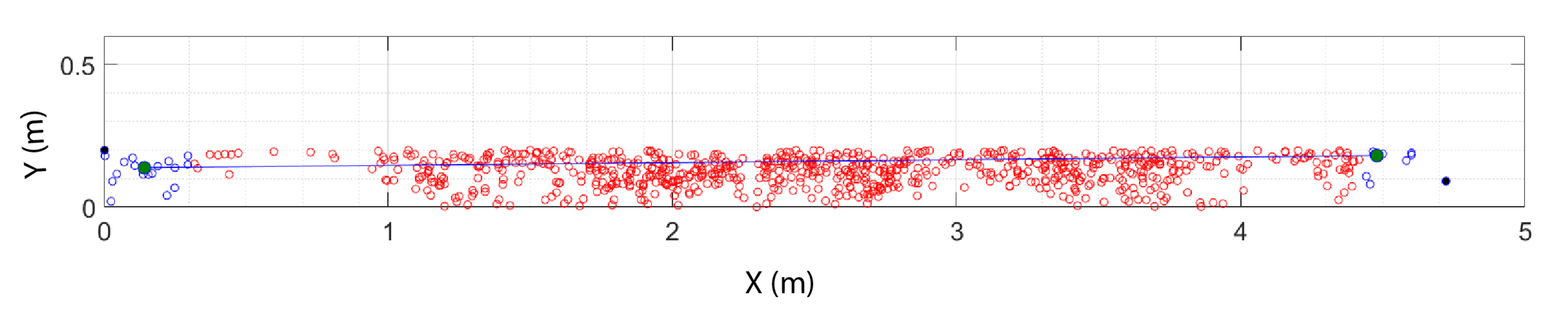
Figure 17.
Drone and car positions registered by global positioning system (GPS) sensors. The light blue icons represent the positions of the drone during the test, the green icons represent the positions of the drone when the picture was captured, and the dark blue icon represents the position of the car.

Figure 18.
Manually selected points of the car (red stars). The purple square represents the GPS sensor position.
Figure 18.
Manually selected points of the car (red stars). The purple square represents the GPS sensor position.

Figure 19.
3D points of the back side (blue), front side (yellow), left side (red), and right side (green) of the car.
Figure 19.
3D points of the back side (blue), front side (yellow), left side (red), and right side (green) of the car.

Figure 20.
Delaunay triangulation surfacing the four sides of the car.

Figure 21.
Complete 3D reconstruction of the car.

Figure 22.
Images of the pseudo-static fire at two different moments: (a) at s and (b) at s.

Figure 23.
3D points computed from the fire stereoscopic images acquired at s.

Figure 24.
Estimated front lines of a pseudo static fire obtained at different instants: s (green dashed line), s (blue dashed line), and s (solid red line).
Figure 24.
Estimated front lines of a pseudo static fire obtained at different instants: s (green dashed line), s (blue dashed line), and s (solid red line).

Figure 25.
Configuration of the fire test area.

Figure 26.
Position of the stereovision device during the test. The x-axis is directed east, the y-axis is directed north, and the z-axis is directed upward.
Figure 26.
Position of the stereovision device during the test. The x-axis is directed east, the y-axis is directed north, and the z-axis is directed upward.

Figure 27.
Ground 3D fire points and propagation plane.

Figure 28.
Image of the fire after a few minutes of propagation.

Figure 29.
Detected frontal fire area and matched points.

Figure 30.
3D fire points.

Figure 31.
Estimated 3D reconstruction of the frontal part of the fire presented in Figure 28.
Figure 31.
Estimated 3D reconstruction of the frontal part of the fire presented in Figure 28.

Figure 32.
Temporal evolution of the fire position at given instants.

Figure 33.
Temporal evolution of the fire position for the whole spread.

Figure 34.
Temporal evolution of the width, height, and depth.

Figure 35.
Temporal evolution of the flame tilt angle.


Table 1.
Comparison between real and estimated measurements of the car.
| Length (m) | Width (m) | Height (m) | Position (lat, lon) | |
|---|---|---|---|---|
| Real | 3.99 | 1.64 | 1.50 | (42.2999911, 9.1755291) |
| Estimated | 3.96 | 1.62 | 1.48 | (42.2999923, 9.1755259) |
| Error | 0.7% | 1.2% | 1.1% | 0.26 m |
Publisher’s Note: MDPI stays neutral with regard to jurisdictional claims in published maps and institutional affiliations. |
© 2020 by the authors. Licensee MDPI, Basel, Switzerland. This article is an open access article distributed under the terms and conditions of the Creative Commons Attribution (CC BY) license (http://creativecommons.org/licenses/by/4.0/).
Share and Cite
MDPI and ACS Style
Ciullo, V.; Rossi, L.; Pieri, A. Experimental Fire Measurement with UAV Multimodal Stereovision. Remote Sens. 2020, 12, 3546. https://0-doi-org.brum.beds.ac.uk/10.3390/rs12213546
AMA Style
Ciullo V, Rossi L, Pieri A. Experimental Fire Measurement with UAV Multimodal Stereovision. Remote Sensing. 2020; 12(21):3546. https://0-doi-org.brum.beds.ac.uk/10.3390/rs12213546
Chicago/Turabian StyleCiullo, Vito, Lucile Rossi, and Antoine Pieri. 2020. "Experimental Fire Measurement with UAV Multimodal Stereovision" Remote Sensing 12, no. 21: 3546. https://0-doi-org.brum.beds.ac.uk/10.3390/rs12213546
Note that from the first issue of 2016, this journal uses article numbers instead of page numbers. See further details here.