Effects of the High-Order Ionospheric Delay on GPS-Based Tropospheric Parameter Estimations in Turkey


1
Department of Geomatics Engineering, Zonguldak Bulent Ecevit University, Zonguldak 67100, Turkey
2
School of Remote Sensing and Geomatics Engineering, Nanjing University of Information Science and Technology, Nanjing 210044, China
3
Shanghai Astronomical Observatory, Chinese Academy of Sciences, Shanghai 200030, China
*
Author to whom correspondence should be addressed.
Remote Sens. 2020, 12(21), 3569; https://0-doi-org.brum.beds.ac.uk/10.3390/rs12213569
Submission received: 14 September 2020
/
Revised: 11 October 2020
/
Accepted: 21 October 2020
/
Published: 31 October 2020
(This article belongs to the Special Issue GNSS High Rate Data for Research of the Ionosphere)
Abstract
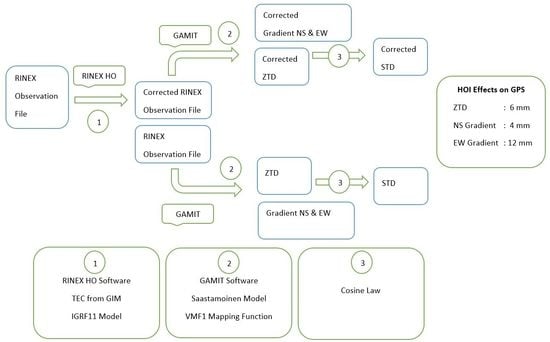
:The tropospheric delay and gradients can be estimated using Global Positioning System (GPS) observations after removing the ionospheric delay, which has been widely used for atmospheric studies and forecasting. However, high-order ionospheric (HOI) delays are generally ignored in GPS processing to estimate atmospheric parameters. In this study, HOI effects on GPS-estimated tropospheric delay and gradients are investigated from two weeks of GPS data in June 2011 at selected GPS stations in Turkey. Results show that HOI effects are up to 6 mm on zenith tropospheric delay (ZTD), 4 mm on the North-South (NS) gradient and 12 mm on the East-West (EW) gradient during this period, but can reach over 30 mm in slant tropospheric delays. Furthermore, the HOI effects on tropospheric delay and gradient are larger in the daytime than the nighttime. Furthermore, HOI effects on tropospheric delay are further investigated on low and high solar activity days. The HOI effects on GPS estimated tropospheric delay and gradients in high solar activity days are higher than those in low solar activity days.
1. Introduction
GPS has been widely used for not only geodetic applications but also atmospheric parameter estimations starting from the late 20th century [1,2,3]. When a GPS signal passes through the atmosphere it is subjected to errors in the atmosphere layers called the ionosphere and the troposphere. Using two different phase or code measurements, the biggest part of the ionospheric error, called first order, can be removed from the equation. However, the second and third orders of ionospheric error are generally neglected in the studies [4,5]. With the advancing technology and necessity of accurate GNSS applications such as position or atmospheric parameter estimation, the high-order ionospheric (HOI) effects on GNSS signals are no longer negligible. At the troposphere, GPS signals are burdened with an error called the tropospheric delay which cannot be removed but modelled. The tropospheric delay consists of two parts: dry and wet delays. The dry part is related to the concentration of gases in the atmosphere, while the wet delay is related to atmospheric parameters such as temperature, pressure, and humidity [2,6].
The tropospheric delay and gradients can be estimated from GPS observations which have been widely used for studies related to atmosphere and forecasting on both global and regional levels using near real-time, real-time, or post-process solutions [7,8,9]. There are several studies on the high-order ionospheric effects on point positioning, such as Hernández-Pajares et al. [10], who studied the impact of HOI effects on the receiver positioning (sub-millimeter), satellite clock (greater than 1 cm), and orbit parameters (several millimeters). Furthermore, in the study of the Hernández-Pajares et al. [11], the impact of the HOI effects and the bending of slant total electron content are investigated. Results show that the total effect is up to 1 cm on satellite Z coordinates and more than 20 ps on satellite clocks. Petrie et al. [12] studied the HOI effect on GPS time series and the reference frame using the 1995–2008 globally reprocessed solutions. Results showed that HOI causes up to 10 mm difference to the ITRF2005 transformation and after transformation up to 0.34 mm/yr residual effects found on vertical site velocities.
Additionally, there are studies related to the effect on atmospheric parameters. Hadas et al. [13] investigated the HOI effects on receiver and satellite parameters along with tropospheric delays and horizontal gradients. According to their findings, the impact of the HOI on tropospheric products are insignificant. However, a study by Zus et al. [14] investigated the effect of the HOI using a few hundred stations in March 2012 and their results revealed that the HOI effects have a considerable impact on the tropospheric parameters, especially on the tropospheric north-gradient component. Recent studies also showed that the HOI effects on zenith wet delay (ZWD) is significant and HOI effects should not be neglected [15,16]. Conflicting results from previous studies, along with the lack of regional case studies, are the main reasons for this study.
In previous studies, only the first term of the ionospheric delay was eliminated [17,18,19], and so to achieve more precise results, HOI corrections are now also needed. The second term of the ionospheric delay is related to several factors, such as the solar cycle, season, and time of day [14,20,21]. Previous studies showed that the first-order ionospheric effect on zenith tropospheric delay (ZTD) can reach up to 30 m, the second-order ionospheric effect up to 2 cm, and the third-order ionospheric effect up to 2 mm [15,22]. Therefore, HOI corrections for GPS applications are needed and mandatory for couple analysis centers or network solutions (e.g., EPN—EUREF Permanent Network).
In this study, HOI effects on GPS tropospheric delay and gradients in Turkey are investigated. In Section 2, the methodology used in the GPS data processing is introduced, HOI effects on tropospheric delay and gradients are presented and discussed in Section 3, and finally, conclusions are given in Section 4.
2. GPS Data Analysis and Methods
In order to estimate HOI effects on tropospheric delay and gradients over Turkey, CORS-TR (TUSAGA-Aktif in Turkish) GPS stations data are used. CORS-TR consists of 146 continuously operating GPS stations. Eight of these stations are nearly co-located with radiosonde stations (Figure 1). Therefore, we utilized these eight stations in this study. In the processing of GPS data, days of the year with low solar activity, 18–24 in 2011, days with high solar activity, 317–323 in 2011, and two randomly selected weeks in June 2011 (166–181) which could represent moderate solar activity are used. In the first step, GPS observation files are corrected for HOI effects with the RINEX_HO software [23]. For this process total electron content (TEC) values are provided from the Global Ionosphere Map (GIM), and geomagnetic field components are taken from the International Geomagnetic Reference Field: 11th generation (IGRF11) model. IGRF11 is provided to predict the large-scale geomagnetic field for five years.
In the second step, using an ionosphere-free combination, the first-order ionospheric error is removed utilizing dual frequency signals, but higher-order ionospheric terms cannot be removed by the combination methods [20,22,24]. The phase (Φi) and code (Pi) observation equations after iono-free combination can be written as Equation (1) [23].
where Li (i = 1, 2) is the frequency, is the geometric distance between the receiver and the satellite, is tropospheric delay, HOI represents the second and third terms of the ionospheric delay, respectively, are metric receiver and satellite clock errors, is wavelength, is the phase ambiguity, and are receiver hardware errors, and are satellite hardware errors, and are the phase and pseudorange residual errors, respectively.
With the usage of iono-free combination on double differenced solution (DD), only the second and the third-order ionospheric terms remain. The second-order term is associated with the geomagnetic field on the ionospheric refractive index, while the third-order term is related to the ray bending error [20,21]. Therefore, the geomagnetic field should be well known in precise applications. The IGRF model provides geomagnetic field components in northward, eastward and vertically downward directions to users [25]. It is not the same along the signal path, so vector representation is utilized for IGRF model data in a generalized coordinate system [26]. For each of the frequency observations, second-order term ( can be computed by Equation (2) [20,21,27,28].
The third-order term ( can be expressed by Equation (3) [29].
where is 80.6 m3/s2, e is 1.60218 × 10⁻¹⁹ Coulomb, is 9.10939 × 10⁻³¹ kg, is the magnitude of the geomagnetic induction vector B, η is constant 0.66, is maximum electron density, and the TEC can be expressed as Equation (4) [23].
where fLi (i = 1, 2) is the GPS frequency, and and (in units of seconds) are, respectively, the receiver and satellite differential code bias. The speed of light in vacuum is represented by c, and represents all remaining residual effects. However, in this study TEC values are interpolated from GIMs using RINEX_HO software along with values. For more detailed information about the HOI and the processing steps of RINEX_HO software, refer to references [15,16,23].
After the HOI correction, corrected and raw observation files are processed with GAMIT/GlobK software separately but with the same strategy [30]. In the processing phase, the iono-free linear combination (L3) of L1&L2 carrier phases, Saastamoinen model and VMF1 (Vienna Mapping Functions I) were used [31,32]. In addition, FES2004 [33] for ocean tide loading, IERS03 [34] for solid earth tide, USNO Bulletin-b for earth orientation parameters and 9 parameter Berne model [35] for solar radiation pressure, and final products of IGS for clock and orbit parameters are used in the DD solution of GAMIT/GlobK software. As output, the tropospheric delay and gradients with half-hour intervals were obtained from both data types. The tropospheric delay ( is expressed as Equation (5).
where and are the tropospheric wet and dry delays, and are the wet and dry zenith delays, are the wet and dry mapping functions, respectively, and is the elevation angle of satellites. The effects of azimuthal asymmetry in the atmospheric delay are included in the model, as expressed as Equation (6).
where is elevation angle of satellite, is the azimuth, are the gradients on the North-South and East-West directions, respectively, and is the mapping function for gradients. As a summary of the processing phase, the only difference between implementing two similar processing strategies is the choice of applying the HOI correction or not. Using the mathematical model expressed in Equation (1), ZTD and gradients are estimated for selected GPS stations. With the carrier-phase ambiguity, station coordinates fixed, and usage of same satellite orbit and clocks, the only parameters that enter the equation as unknowns are the ZTD, gradient components . Therefore, the vector of estimated parameters for the DD solution can be expressed as Equation (7).
3. Results and Discussion
3.1. HOI Effects on GPS ZTD and Gradients
CORS-TR GPS Stations data in Turkey on the days 167–180 in 2011, were corrected for the HOI effects using the RINEX-HO software and corrected observation files for high-order ionospheric effects were obtained. Then, corrected and raw observation files were processed by GAMIT/GlobK software, and ZTD values were estimated for each station to investigate HOI effects on GPS estimated ZTD values. The mean and root mean square (RMS) values of the differences of computed ZTD values are presented in Table 1.
While the mean values of the ZTD differences at all the GPS stations are close, the RMS of the DIYB station is relatively higher than the other stations. After further inspecting the ZTD differences at the DIYB station, it was found that the HOI effects on ZTD time series for DIYB station reaches up to 6 mm (Figure 2). Peaks in the differences between two ZTD time series could be related to the latitude of the DIYB station and/or the TEC activities on specific days.
As shown in Equation (5), the tropospheric delay consists of wet and dry parts. The dry part is computed from the natural gases law and the wet part is estimated by subtracting the dry part from the total zenith delay. The amount of precipitable water vapor can be estimated from the wet delay using the function of surface temperature. Since the GPS meteorology studies are always aimed at establishing better accuracy to estimate precipitable water vapor, which is directly related to the wet part of the zenith delay, higher-order ionospheric delays should no longer be neglected. Apart from the estimated ZTD values, NS and EW gradients are also estimated. Tropospheric delay gradients are continuously varying and affecting the baseline lengths and positioning [36,37]. Here, we further investigate HOI effects on tropospheric gradients. The mean and RMS values of the differences of computed gradient values are presented in Table 2.
While the differences of the mean values of the NS gradient at all the GPS stations are around 1 mm, differences in the mean values of the EW gradient are very low, except for the ERZR station. RMS of the DIYB and ERZR stations are relatively higher than at the other stations. At the DIYB GPS station with the highest RMS value, NS and EW gradients vary between −30 and 30 mm. Figure 3 shows tropospheric gradients on the NS and EW directions at the DIYB GPS station. However, EW gradient RMS values are at the western side of Turkey (ISPT, ISTN, and IZMI) which is lower than the eastern stations. HOI effects can result in up to 4 and 12 mm of change in NS and EW gradients, respectively (Figure 3). Apart from the DIYB station, mean values of both NS and EW gradient differences confirm previous studies which state that NS gradients are more likely to be affected by HOI delays than EW gradients [15].
3.2. HOI Effects During the Daytime and Nighttime
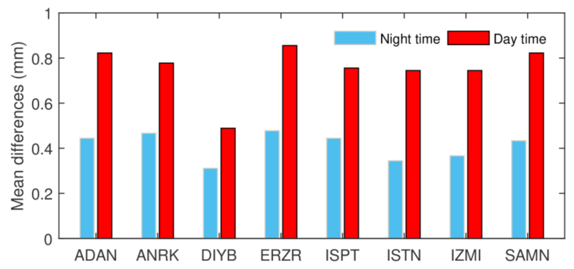
HOI effects are related to the solar activity and ionospheric conditions as well as the time of day which is directly related to the sun itself. Total electron content is the main parameter of ionospheric delay. While the TEC values during the daytime are higher than at nighttime, it is expected that HOI effects on GPS estimated ZTD should also be higher during the daytime. In Figure 4, ZTD values estimated from with and without HOI correction, along with their differences for nighttime (00:00–04:00 UT) and daytime (12:00–16:00 UT), at ANRK GPS station on day 167 in 2011, are plotted. The RMS increases from 0.48 mm at nighttime to 0.78 mm during the daytime. This effect is significant for not only ANRK station but also for other GPS stations.
Mean differences between two data sets with and without HOI correction shows the change from nighttime to daytime (Figure 5), and the conclusions are the same. Mean differences are nearly 0.4 mm in the nighttime and around 0.8 mm during the daytime for each station.
3.3. HOI Effects during the High and Low Solar Activities
HOI effects depend on solar activity, geomagnetic, and ionospheric conditions [16]. Solar storms that occur on the sun are the major disturbance of the earth’s magnetosphere with the efficient exchange of energy from the sun to the earth’s atmosphere. These disturbances are critical for atmospheric studies and recorded in a different type of index. Energy currents in the magnetosphere follow a magnetic field and connect to dense currents in the auroral ionosphere. F10.7 flux is the most reliable solar activity indicator [38]. Daily averages of solar activity for 2011 are shown in Figure 6.
The effects of the high-order ionospheric delay on ZTD values are investigated during high and low solar activities. Here, one week of GPS data on days 18–24 in 2011 with low solar activity, and days 317–323 in 2011 with high solar activity, were processed. Results show that large HOI effects occur during high solar activity, while HOI effects are much smaller on low solar activity days (Figure 7).
Furthermore, the HOI effects on tropospheric gradients are further investigated during low and high solar activity days. The RMS values of gradient differences are higher on high solar activity days than ones on low solar activity days, for all GPS stations (Figure 8). As an example, the RMS of the North-South gradient differences at ANRK station is 0.86 mm on low solar activity days and reaches up to 2.74 mm on high solar activity days. The ERZR station has maximum effect at the RMS of East-West gradient differences with 0.69 mm on low solar activity days, reaching up to 2.20 mm on high solar activity days. All of the stations show consistent results with the RMS of NS gradient differences being higher than the RMS of EW gradient differences on high and low solar activity days.
3.4. HOI Effect on Slant Tropospheric Delay
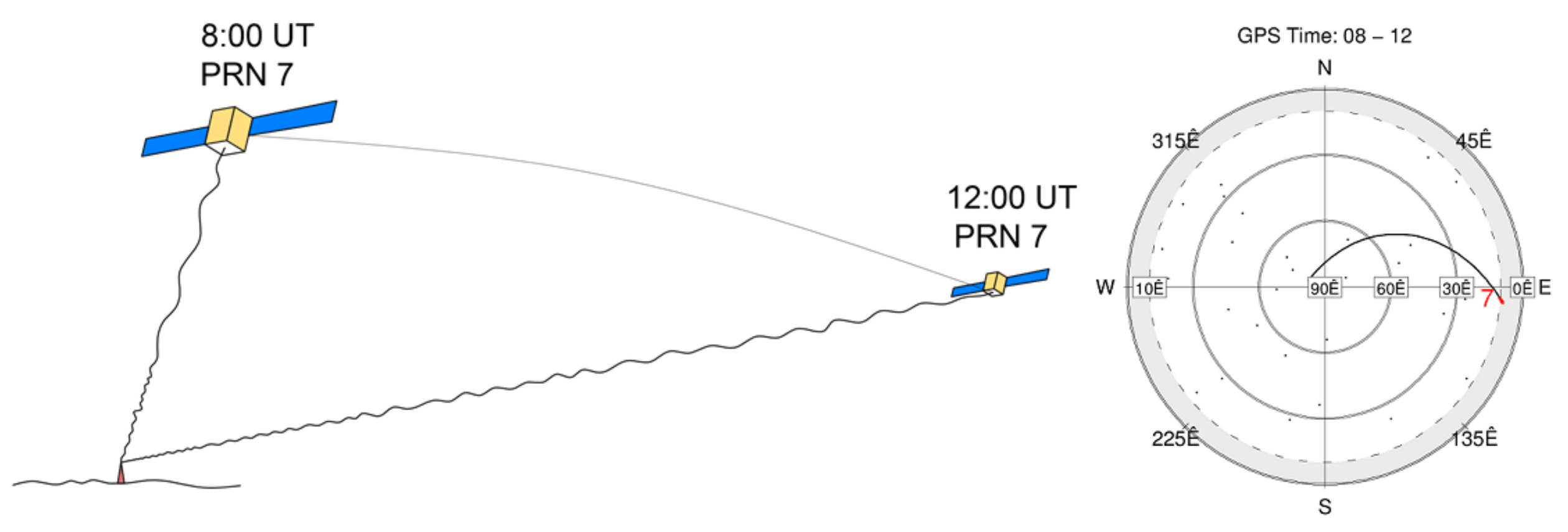
When the GPS satellite elevation angle is low, the more tropospheric delay will be induced due to the travel length of the signal at the troposphere. Computing ZTD values requires the usage of mapping functions to convert slant delays to zenith delays. Here, the HOI effects on slant tropospheric delay (STD) are further investigated. In this case, STD is also estimated with and without HOI correction. As an example, during the four hours, satellite PRN 7 on ANRK station starts to be seen with 293°13′ azimuth and 71°79′ elevation angles at 8:00 UT, then arrives at the 104°80′ azimuth and 11°03′ elevation angles at 12:00 UT (Figure 9).
As seen in Figure 9, the satellite elevation has been decreasing for the satellite PRN 7 from 8:00 UT to 12:00 UT. Tropospheric delay is directly related to the elevation angle of the satellite due to signal travelling length at the troposphere. Therefore, the lower elevation angle means higher tropospheric delay. As an example, Figure 10 shows HOI effects on GPS STD for PRN 7 on day 167 in 2011 at ANRK station. The HOI effect on the STD was about 33 mm including uncertainties when the GPS satellite elevation angle was at 11°03′ degrees. Therefore, the HOI has a large effect on slant tropospheric delay estimation with approximately a few centimeters at low satellite angles.
4. Conclusions
This study aimed to investigate the high-order ionospheric effects on GPS estimated tropospheric delay and gradients in Turkey. In the processing phase, three GPS data sets which are days 18–24 in 2011 with low solar activity, days 317–323 in 2011 with high solar activity, and two randomly selected weeks in June 2011 (days 166–181) which could represent moderate solar activity, were used. Two different results were obtained by applying HOI corrections and neglecting HOI corrections which are compared at different steps.
Even on considerably moderate solar activity days, when mean ZTD differences are at sub-millimeter level, HOI effects can reach up to 6 mm. Apart from the DIYB station, NS gradients are more likely to be affected from HOI delays than the EW gradients. On a randomly selected day, during the daytime with the sun shining, HOI effects on tropospheric delay are much more than at nighttime, with the mean differences around 0.4 mm at nighttime and around 0.8 mm during the daytime for each station.
It can be seen from the RMS of ZTD differences (Figure 7) and gradients (Figure 8) that on high solar activity days, the effect of the HOI is more than double that on low solar activity days. Additionally, HOI effects on slant tropospheric delay are higher at low elevation angles and can reach up to 30 mm. Therefore, the high-order ionospheric delay has considerable effect on tropospheric delay and gradient estimations even in mid-latitudes. HOI effects depend on solar activity, geomagnetic and ionospheric conditions. These effects are much smaller when compared to the first-order ionospheric effects. Therefore, HOI effects are generally ignored in GPS applications. However, to achieve higher accuracy and precision in GPS applications, HOI effects should be corrected, especially on high solar activity days.
Author Contributions
V.A. and S.J. designed the experiment; G.G. and V.A. performed the experiment and analyzed the data. V.A., G.G., S.J., and S.H.K., contributed to the writing of the paper. All authors have read and agreed to the published version of the manuscript.
Funding
This research received no external funding.
Acknowledgments
This study is conducted at the Zonguldak Bülent Ecevit University as a part of a Master degree thesis titled “High Order Ionospheric Effects on GPS Tropospheric Parameter and Coordinate Estimations”. The authors are grateful to the organizations that provided the data, including the International GNSS Service, the EUREF Permanent Network and, the General Directorate of Mapping and General Directorate of Land Registry and Cadastre (Turkey).
Conflicts of Interest
The authors declare no conflict of interest.
References
- Bevis, M.; Businger, S.; Herring, T.A.; Rocken, C.; Anthes, R.A.; Ware, R.H. GPS meteorology: Remote sensing of atmospheric water vapor using the global positioning system. J. Geophys. Res. Space Phys. 1992, 97, 15787–15801. [Google Scholar] [CrossRef]
- Bevis, M.; Businger, S.; Chiswell, S.; Herring, T.A.; Anthes, R.A.; Rocken, C.; Ware, R.H. GPS Meteorology: Mapping Zenith Wet Delays onto Precipitable Water. J. Appl. Meteorol. Climatol. 1994, 33, 379–386. [Google Scholar] [CrossRef]
- Businger, S.; Chiswell, S.R.; Bevis, M.; Duan, J.; Anthes, R.A.; Rocken, C.; Ware, R.; Exner, M.; Vanhove, T.; Solheim, F.S. The Promise of GPS in Atmospheric Monitoring. Bull. Am. Meteorol. Soc. 1996, 77, 5–18. [Google Scholar] [CrossRef] [Green Version]
- Yuan, Y.; Zhang, K.; Rohm, W.; Choy, S.; Norman, R.; Wang, C.S. Real-time retrieval of precipitable water vapor from GPS precise point positioning. J. Geophys. Res. Atmos. 2014, 119, 10044–10057. [Google Scholar] [CrossRef]
- Gurbuz, G.; Jin, S. Long-time variations of precipitable water vapour estimated from GPS, MODIS and radiosonde observations in Turkey. Int. J. Clim. 2017, 37, 5170–5180. [Google Scholar] [CrossRef]
- Rocken, C.; van Hove, T.; Johnson, J.; Solheim, F.; Ware, R.; Bevis, M.; Chiswell, S.; Businger, S. GPS/STORM—GPS Sensing of Atmospheric Water Vapor for Meteorology. J. Atmos. Ocean. Technol. 1995, 12, 468–478. [Google Scholar] [CrossRef]
- Jin, S.; Park, J.U.; Cho, J.H.; Park, P.H. Seasonal variability of GPS-derived zenith tropospheric delay (1994–2006) and climate implications. J. Geophys. Res. Space Phys. 2007, 112. [Google Scholar] [CrossRef]
- Jin, S.; Li, Z.; Cho, J. Integrated Water Vapor Field and Multiscale Variations over China from GPS Measurements. J. Appl. Meteorol. Clim. 2008, 47, 3008–3015. [Google Scholar] [CrossRef]
- Jin, S.; Luo, O. Variability and Climatology of PWV from Global 13-Year GPS Observations. IEEE Trans. Geosci. Remote. Sens. 2009, 47, 1918–1924. [Google Scholar] [CrossRef]
- Hernández-Pajares, M.; Juan, J.M.; Sanz, J.; Orús, R. Second-order ionospheric term in GPS: Implementation and impact on geodetic estimates. J. Geophys. Res. Space Phys. 2007, 112. [Google Scholar] [CrossRef]
- Hernández-Pajares, M.; Aragón-Ángel, À.; Defraigne, P.; Bergeot, N.; Prieto-Cerdeira, R.; García-Rigo, A. Distribution and mitigation of higher-order ionospheric effects on precise GNSS processing. J. Geophys. Res. Solid Earth 2014, 119, 3823–3837. [Google Scholar] [CrossRef] [Green Version]
- Petrie, E.J.; King, M.A.; Moore, P.; Lavallée, D.A. Higher-order ionospheric effects on the GPS reference frame and velocities. J. Geophys. Res. Space Phys. 2010, 115. [Google Scholar] [CrossRef] [Green Version]
- Hadas, T.; Krypiak-Gregorczyk, A.; Hernández-Pajares, M.; Kapłon, J.; Paziewski, J.; Wielgosz, P.; García-Rigo, A.; Kazmierski, K.; Sośnica, K.; Kwasniak, D.; et al. Impact and Implementation of Higher-Order Ionospheric Effects on Precise GNSS Applications. J. Geophys. Res. Solid Earth 2017, 122, 9420–9436. [Google Scholar] [CrossRef]
- Zus, F.; Deng, Z.; Wickert, J. The impact of higher-order ionospheric effects on estimated tropospheric parameters in Precise Point Positioning. Radio Sci. 2017, 52, 963–971. [Google Scholar] [CrossRef] [Green Version]
- Zhang, Z.; Guo, F.; Zhang, X. The Effects of Higher-Order Ionospheric Terms on GPS Tropospheric Delay and Gradient Estimates. Remote Sens. 2018, 10, 1561. [Google Scholar] [CrossRef] [Green Version]
- Zhang, S.; Fang, L.; Wang, G.; Li, W. The impact of second-order ionospheric delays on the ZWD estimation with GPS and BDS measurements. GPS Solut. 2020, 24, 1–11. [Google Scholar] [CrossRef]
- Jin, S.; Occhipinti, G.; Jin, R. GNSS ionospheric seismology: Recent observation evidences and characteristics. Earth Sci. Rev. 2015, 147, 54–64. [Google Scholar] [CrossRef]
- Jin, S.; Jin, R.; Li, D. Assessment of BeiDou differential code bias variations from multi-GNSS network observations. Ann. Geophys. 2016, 34, 259–269. [Google Scholar] [CrossRef] [Green Version]
- Li, J.; Jin, S. High-order ionospheric effects on electron density estimation from Fengyun-3C GPS radio occultation. Ann. Geophys. 2017, 35, 403–411. [Google Scholar] [CrossRef] [Green Version]
- Bassiri, S.; Hajj, G.A. Higher-order ionospheric effects on the global positioning system observables and means of modeling them. Manuscr. Geod. 1993, 18, 280–289. [Google Scholar]
- Kedar, S.; Hajj, G.A.; Wilson, B.D.; Heflin, M.B. The effect of the second order GPS ionospheric correction on receiver positions. Geophys. Res. Lett. 2003, 30, 1829. [Google Scholar] [CrossRef]
- Brunner, F.K.; Gu, M. An improved model for the dual frequency ionospheric correction of GPS observations. Manuscr. Geod. 1991, 16, 205–214. [Google Scholar]
- Marques, H.A.; Monico, J.F.G.; Aquino, M. RINEX_HO: Second- and third-order ionospheric corrections for RINEX observation files. GPS Solut. 2011, 15, 305–314. [Google Scholar] [CrossRef]
- King, R.W.; Collins, J.; Masters, E.M.; Rizos, C.; Stolz, A. Surveying with GPS; Monograph No. 9; School of Surveying, University of New South Wales: Kensington, NSW, Australia, 1985. [Google Scholar]
- Mandea, M.; Macmillan, S. International Geomagnetic Reference Field—The eighth generation. Earth Planets Space 2000, 52, 1119–1124. [Google Scholar] [CrossRef] [Green Version]
- Arfken, G. Mathematical Methods for Physicists; Elsevier: Amsterdam, The Netherlands, 1985. [Google Scholar]
- Odijk, D. Fast Precise GPS Positioning in the Presence of Ionospheric Delays. Ph.D. Thesis, Faculty of Civil Engineering and Geosciences, Delft University of Technology, Delft, The Netherlands, 2002. [Google Scholar]
- Hoque, M.M.; Jakowski, N. Higher order ionospheric effects in precise GNSS positioning. J. Geod. 2006, 81, 259–268. [Google Scholar] [CrossRef]
- Hartmann, G.K.; Leitinger, R. Range errors due to ionospheric and tropospheric effects for signal frequencies above 100 MHz. J. Geod. 1984, 58, 109–136. [Google Scholar] [CrossRef]
- Herring, T.A.; King, R.W.; McClusky, S.C. Introduction to GAMIT/GLOBK 10.6; Massachusetts Institute of Technology: Cambridge, MA, USA, 2015. [Google Scholar]
- Saastamoinen, J. Atmospheric correction for the troposphere and stratosphere in radio ranging of satellites. In The Use of Artificial Satellites for Geodesy; Geophysical monograph series 15; American Geophysical Union: Washington, DC, USA, 1972; pp. 247–251. [Google Scholar] [CrossRef]
- Boehm, J. Vienna mapping functions in VLBI analyses. Geophys. Res. Lett. 2004, 31. [Google Scholar] [CrossRef]
- Lyard, F.; Lefevre, F.; Letellier, T.; Francis, O. Modelling the global ocean tides: Modern insights from FES2004. Ocean. Dyn. 2006, 56, 394–415. [Google Scholar] [CrossRef]
- McCarthy, D.D.; Petit, G. IERS Conventions (2003); IERS Technical Note 32; Verlag des Budesamts fur Kartographie und Geodasie: Frankfurt, Germany, 2004. [Google Scholar]
- Springer, T.A.; Beutler, G.; Rothacher, M. A New Solar Radiation Pressure Model for GPS Satellites. GPS Solut. 1999, 2, 50–62. [Google Scholar] [CrossRef]
- Davis, J.L.; Elgered, G.; Niell, A.E.; Kuehn, C.E. Ground-based measurement of gradients in the “wet” radio refractivity of air. Radio Sci. 1993, 28, 1003–1018. [Google Scholar] [CrossRef]
- Teke, K.; Böhm, J.; Nilsson, T.; Schuh, H.; Steigenberger, P.; Dach, R.; Heinkelmann, R.; Willis, P.; Haas, R.; García-Espada, S.; et al. Multi-technique comparison of troposphere zenith delays and gradients during CONT08. J. Geod. 2011, 85, 395–413. [Google Scholar] [CrossRef] [Green Version]
- Tapping, K.F. The 10.7 cm solar radio flux (F10.7). Space Weather 2013, 11, 394–406. [Google Scholar] [CrossRef]
Figure 1.
GPS and radiosonde stations distribution.

Figure 2.
Time series of ZTD values (top) and differences (bottom) at the DIYB GPS station on days 168–180 in 2011.
Figure 2.
Time series of ZTD values (top) and differences (bottom) at the DIYB GPS station on days 168–180 in 2011.

Figure 3.
NS (left) and EW (right) gradients time series (top) and differences (bottom) at the DIYB GPS station on days 168–180 in 2011.
Figure 3.
NS (left) and EW (right) gradients time series (top) and differences (bottom) at the DIYB GPS station on days 168–180 in 2011.

Figure 4.
ZTD time series (top) and differences (bottom) at ANRK station during the night (left) and the day (right) on day 167 in 2011.
Figure 4.
ZTD time series (top) and differences (bottom) at ANRK station during the night (left) and the day (right) on day 167 in 2011.

Figure 5.
Daytime and nighttime mean ZTD differences on days 167–180 in 2011.

Figure 6.
Time series of daily average values of the Solar 10.7 cm flux for 2011.

Figure 7.
RMS of ZTD differences on low (days 18–24) and high (days 317–323) solar activity days.

Figure 8.
RMS of NS (left) and EW (right) gradient differences during low (days 18–24) and high (days 317–323) solar activity days.
Figure 8.
RMS of NS (left) and EW (right) gradient differences during low (days 18–24) and high (days 317–323) solar activity days.

Figure 9.
PRN 7 satellite visibility on day 167 in 2011 at ANRK station.

Figure 10.
Elevation angle (top), time series of slant tropospheric delay (STD) (middle) and STD differences (bottom) estimated from PRN 7 GPS satellite on day 167 in 2011 at ANRK station.
Figure 10.
Elevation angle (top), time series of slant tropospheric delay (STD) (middle) and STD differences (bottom) estimated from PRN 7 GPS satellite on day 167 in 2011 at ANRK station.


Table 1.
Mean and root mean square (RMS) values of the zenith tropospheric delay (ZTD) differences on days 167–180 in 2011.
Table 1.
Mean and root mean square (RMS) values of the zenith tropospheric delay (ZTD) differences on days 167–180 in 2011.
| Stations | Mean (mm) | RMS (mm) |
|---|---|---|
| ADAN | 0.24 | 0.48 |
| ANRK | 0.26 | 0.56 |
| DIYB | 0.27 | 0.69 |
| ERZR | 0.27 | 0.56 |
| ISPT | 0.24 | 0.45 |
| ISTN | 0.22 | 0.45 |
| IZMI | 0.23 | 0.47 |
| SAMN | 0.24 | 0.45 |
Table 2.
Mean and RMS values of the NS and EW gradients differences on days 168–180 in 2011.
| GPS | NS Gradient (mm) | EW Gradient (mm) | ||
|---|---|---|---|---|
| Stations | Mean | RMS | Mean | RMS |
| ADAN | 1.00 | 1.09 | 0.43 | 1.39 |
| ANRK | 0.78 | 1.17 | 0.02 | 1.58 |
| DIYB | 1.02 | 1.29 | −0.03 | 2.12 |
| ERZR | 0.82 | 1.01 | 0.86 | 1.83 |
| ISPT | 0.99 | 1.11 | 0.14 | 0.70 |
| ISTN | 0.92 | 1.06 | −0.02 | 0.52 |
| IZMI | 0.83 | 1.09 | 0.13 | 0.77 |
| SAMN | 0.99 | 1.04 | 0.55 | 1.41 |
Publisher’s Note: MDPI stays neutral with regard to jurisdictional claims in published maps and institutional affiliations. |
© 2020 by the authors. Licensee MDPI, Basel, Switzerland. This article is an open access article distributed under the terms and conditions of the Creative Commons Attribution (CC BY) license (http://creativecommons.org/licenses/by/4.0/).
Share and Cite
MDPI and ACS Style
Akgul, V.; Gurbuz, G.; Kutoglu, S.H.; Jin, S. Effects of the High-Order Ionospheric Delay on GPS-Based Tropospheric Parameter Estimations in Turkey. Remote Sens. 2020, 12, 3569. https://0-doi-org.brum.beds.ac.uk/10.3390/rs12213569
AMA Style
Akgul V, Gurbuz G, Kutoglu SH, Jin S. Effects of the High-Order Ionospheric Delay on GPS-Based Tropospheric Parameter Estimations in Turkey. Remote Sensing. 2020; 12(21):3569. https://0-doi-org.brum.beds.ac.uk/10.3390/rs12213569
Chicago/Turabian StyleAkgul, Volkan, Gokhan Gurbuz, Senol Hakan Kutoglu, and Shuanggen Jin. 2020. "Effects of the High-Order Ionospheric Delay on GPS-Based Tropospheric Parameter Estimations in Turkey" Remote Sensing 12, no. 21: 3569. https://0-doi-org.brum.beds.ac.uk/10.3390/rs12213569
Note that from the first issue of 2016, this journal uses article numbers instead of page numbers. See further details here.