Automatic Mapping of Rice Growth Stages Using the Integration of SENTINEL-2, MOD13Q1, and SENTINEL-1

Abstract

Rice (Oryza sativa L.) is a staple food crop for more than half of the world’s population. Rice production is facing a myriad of problems, including water shortage, climate, and land-use change. Accurate maps of rice growth stages are critical for monitoring rice production and assessing its impacts on national and global food security. Rice growth stages are typically monitored by coarse-resolution satellite imagery. However, it is difficult to accurately map due to the occurrence of mixed pixels in fragmented and patchy rice fields, as well as cloud cover, particularly in tropical countries. To solve these problems, we developed an automated mapping workflow to produce near real-time multi-temporal maps of rice growth stages at a 10-m spatial resolution using multisource remote sensing data (Sentinel-2, MOD13Q1, and Sentinel-1). This study was investigated between 1 June and 29 September 2018 in two (wet and dry) areas of Java Island in Indonesia. First, we built prediction models based on Sentinel-2, and fusion of MOD13Q1/Sentinel-1 using the ground truth information. Second, we applied the prediction models on all images in area and time and separation between the non-rice planting class and rice planting class over the cropping pattern. Moreover, the model’s consistency on the multitemporal map with a 5–30-day lag was investigated. The result indicates that the Sentinel-2 based model classification gives a high overall accuracy of 90.6% and the fusion model MOD13Q1/Sentinel-1 shows 78.3%. The performance of multitemporal maps was consistent between time lags with an accuracy of 83.27–90.39% for Sentinel-2 and 84.15% for the integration of Sentinel-2/MOD13Q1/Sentinel-1. The results from this study show that it is possible to integrate multisource remote sensing for regular monitoring of rice phenology, thereby generating spatial information to support local-, national-, and regional-scale food security applications.

1. Introduction

Regular monitoring of the paddy area is vital as rice production supports rural livelihoods in Asia, where more than 1.21 billion tonnes of rice were harvested to feed 4.56 billion people in 2018 [1,2]. The rice production often struggles with the effects of climate change [3,4], water shortage [5,6], inadequate machinery supplies in developing countries [7], and soil degradation [8], which in turn requires intensified monitoring to ensure sustained food production. The common practice of monitoring rice crops in Indonesia is by using local government officers at a sub-district level to collect data based on field visits and information provided by the farmers. This data is expensive to collect, non real-time, and inefficient to handle spatio-temporal changes in rice-producing areas [9,10,11]. Moreover, the paddy area needs to be monitored in near-time due to the need for a continuous water supply from irrigation canals and fertiliser inputs at critical stages [12]. Thus, timely and accurate information on rice growth stages is vital for planning and management of the rice farming system, which is critical for sustainable food security at the regional and national scale [13,14].

Remote sensing can offer cost-effective near real-time solutions to analyse land-use changes [15,16,17], cropping patterns [18,19,20,21,22], growth stages [21,23,24], and crop detection over large areas [25]. Previous studies have widely used coarse-resolution multitemporal optical imagery, such as Moderate Resolution Imaging Spectrometer (MODIS) [26,27,28,29,30], for rice monitoring. MODIS has a significant advantage of daily revisit time and able to generate vegetation indices, such as enhanced vegetation index (EVI) and normalized different vegetation index (NDVI). These indices can be used to quantify rice growth stages accurately, and therefore to recreate a temporal evolution of rice production. This data can be fed in to establish regional and national productivity of rice yield inventories [29,31,32]. However, most of the other optical satellites have less frequent visit times, and they are prone to cloud cover and shadow, resulting in gaps in the temporal data, particularly in monsoon season [33]. Additionally, their medium to coarse spatial resolution (>250 m) hampers the capability to discriminate the rice growth stages within paddy fields. Moreover, paddy rice fields are often highly fragmented, resulting in mixed pixels. Some prior studies show that single-date rice monitoring with Landsat 7/8 can be done with better accuracy [24,34,35] with a revisited time of 16 days, which is difficult to get clear data useful at the operational level.

To avoid the cloud interference, microwave or synthetic aperture radar (SAR) data from RADARSAT [36,37], ALOS-PALSAR [38,39], and Sentinel-1 [40,41,42,43,44,45], have been explored for rice mapping. The backscattering of the microwave radiation can be used to detect the rice cropping pattern due to phenological changes of the rice canopy structure having characteristic microwave scattering properties [46]. The previous studies on the mapping of rice growth stages are limited to identifying rice/non-rice area [47,48,49], and the cropping pattern using various sensors [50]. Rudiyanto, Minasny, Shah, Che Soh, Arif, and Indra Setiawan [21] demonstrated the detection of rice phenology in Indonesia and Malaysia rice fields, using hierarchical clustering with vertical-horizontal backscatter from Sentinel-1. On the other hand, Phung et al. [51] were able to correlate between incident angles of backscattering and day of planting based on smoothed VH backscattering intensity images. These studies have utilised the fact that the inundation and vegetative rice growth stages typically have the lowest backscattering intensity due to the flooded soil that reflects the radar energy specularly away from the sensor. As the rice grows, the backscattering intensity becomes higher when the rice canopy is established (e.g., reproductive phase) as the canopy can give double-bounce scattering [52,53]. Finally, the backscattering intensity becomes lower again after harvesting due to a loss of biomass [54]. The utility of RADAR for rice growth stage monitoring can also benefit from the frequent satellite revisit times, and penetration through cloud cover affected by many tropical countries. The only global and free dataset of RADAR is provided by Sentinel-1 satellite imagery. Other RADAR-capable satellites, such as ALOS-PALSAR and TerraSAR-X, are limited in uses or available via paid subscriptions. Moreover, the speckle noise issue can be a problem in complex land-use [55] and can be minimized with the deep learning approach [56,57]. Importantly, microwave remote sensing has a significant time lag to be analysed near-real-time due to its slow processing time and high demand for local knowledge to classify the rice growth stages [21]. Moreover, the short time is vital for rice mapping for validating the rice production prediction on a national or local scale.

Considering the advantages from both optical and radar images, combining multiple remote sensing data (data fusion) has the potential to improve the accuracy with high temporal coverage. The fusion between active and passive remote sensing have been adopted [58,59,60,61], to overcome the missing data, and have higher accuracies due to the ability to distinguish specific crop area, especially near water bodies. According to Schmitt and Zhu [62], there are three types of data fusion: (1) raw data fusion, (2) feature extraction fusion, and (3) decision-making level. Feature extraction fusion is more attractive than the others because the fusion process can be carried out with multiple images with different temporal and spatial resolution. The feature fusion uses similar objects from multiple sources that are combined for further assessment. For example, Park et al. [63] developed a method by combining the data of Landsat, MODIS, and ALOS-PALSAR to map paddy area in South Korea, which increased the accuracy by 6–9%, compared to individual sensor information. Similarly, Cai et al. [64] reported high accuracy for mapping rice paddy area in China with multiple sensors (Sentinel-1/Sentinel-2/MODIS). The resultant high accuracy is due to the strong correlation between the leaf area index (LAI) and biomass with cross-polarization of microwave backscattering [65]. To date, the study of integration between optical and radar-based imagery on rice growth stages classification is not investigated thoroughly on the feature extraction and decision-making fusion level to increase accuracy.

Considering some limitations of previous studies, the actual demand for near-real time rice growth stage prediction models using remote sensing is high. Thus, this study aimed to develop an automatic workflow for generating 10-m-resolution multitemporal maps of rice growth stages by combining Sentinel-2, MOD13Q1, and Sentinel-1 imagery. The result of this study, both the method and the map products, can be used for mapping at national and regional scales to ensure food security and production with timely and accurate spatial information using multiple remote sensing data sources.

2. Background, Study Area, and Data

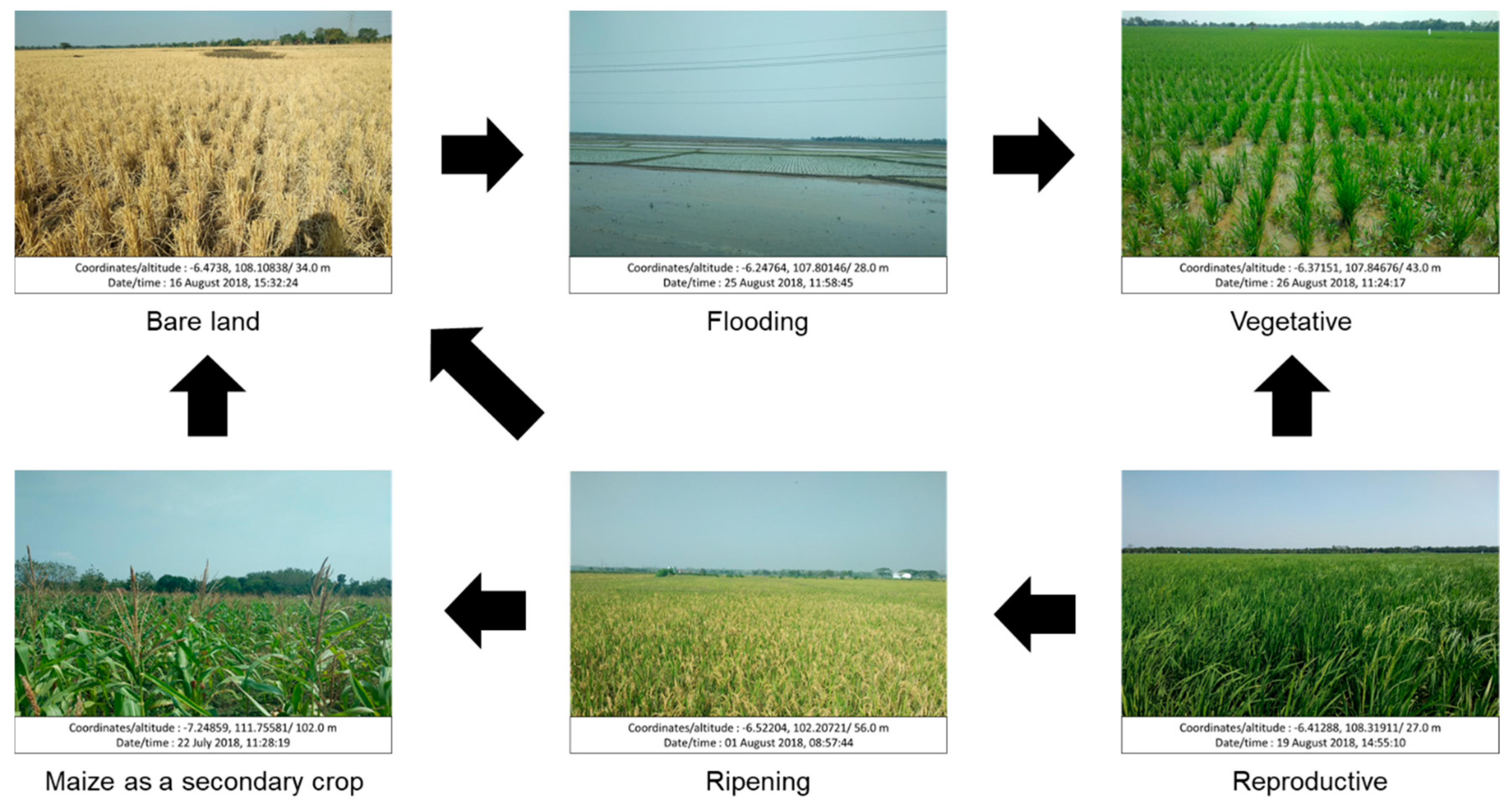
2.1. Rice Growth Stages

The growth stage of paddy rice in Asia, particularly Indonesia, can be split into five classes, which reflect the rice cultivation practices in any given time [66,67,68]. First, the bare land area is filled by water (flooding) and ploughed for (15–25 days) depending on the water irrigation schedule (Figure 1). The second stage is the vegetative stage, which the rice grows from seedling emergence until panicle development (55–65 days; Figure 1). The third stage is the reproductive stage where the leaf stem bulges with the panicle, also known as the booting stage (20–25 days; Figure 1). Flowering and pollination also occur in this stage. The final stage is the ripening stage, which includes fertilisation, the grain is filling/expanding, and the paddy grain becomes dry-brown (30–35 days; Figure 1). The total cultivation time is 120–150 days, depending on the varieties. Intercrops, growing other crops (maize, soybean, green beans) between the rice crop, are also adopted in some areas.

2.2. Study Area

In this study, we chose two distinctive regions with different climates (wet and dry area) and fragmented paddy area from Java Island, Indonesia (Figure 2). The West Area is located on West Java, which represents the paddy area, mainly irrigated area and low land, while the East Area is located with larger rain-fed paddy field and have a high fragmented area. Both areas have a monsoon climate with two seasons: the wet season and the dry season [69]. The wet season is from October to March, and the dry season is April to September (see Supplementary Figure S1). Typically, short-duration varieties, such as IR64, Ciherang, of glutinous rice are widely adopted in this area [19,21].

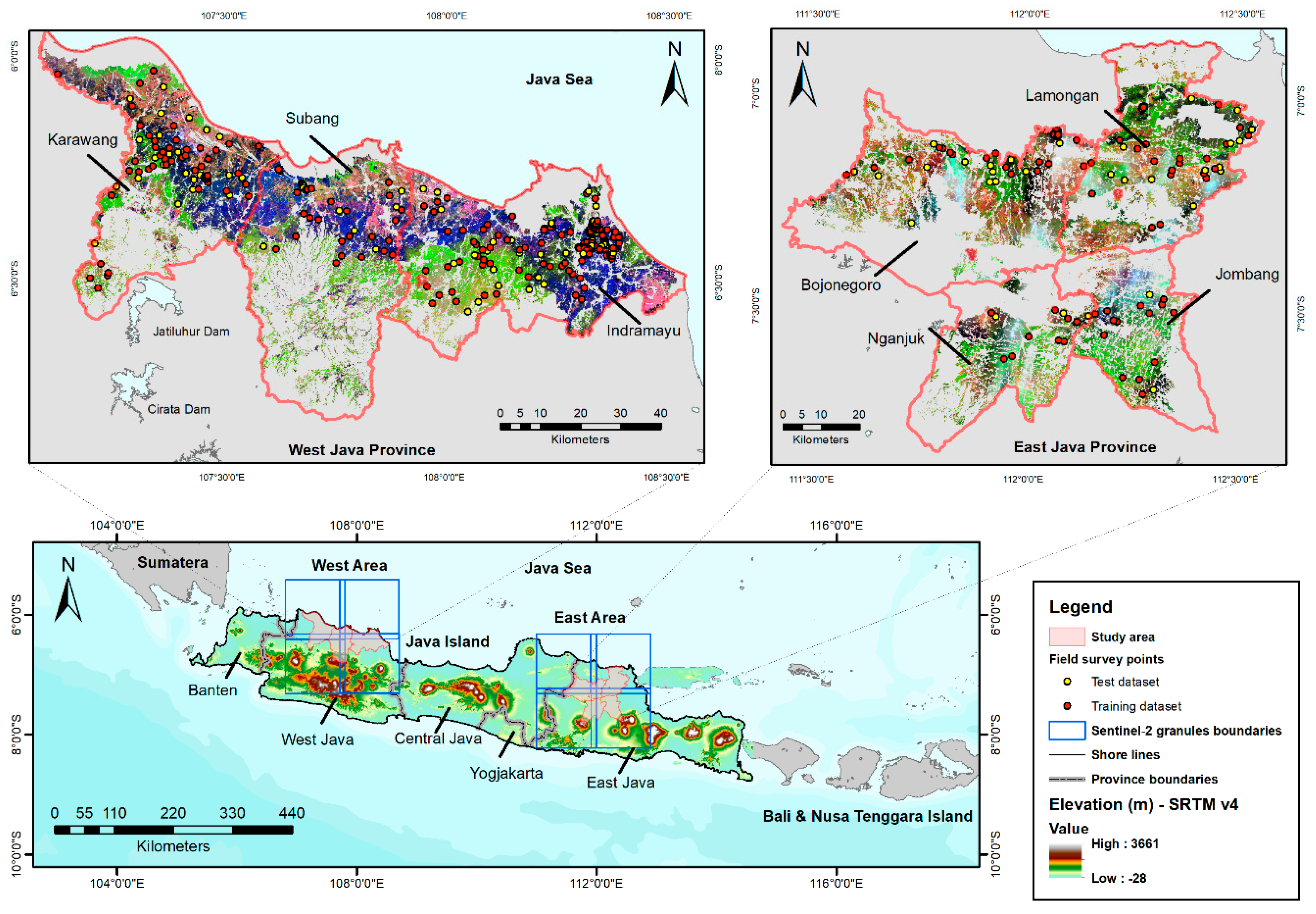
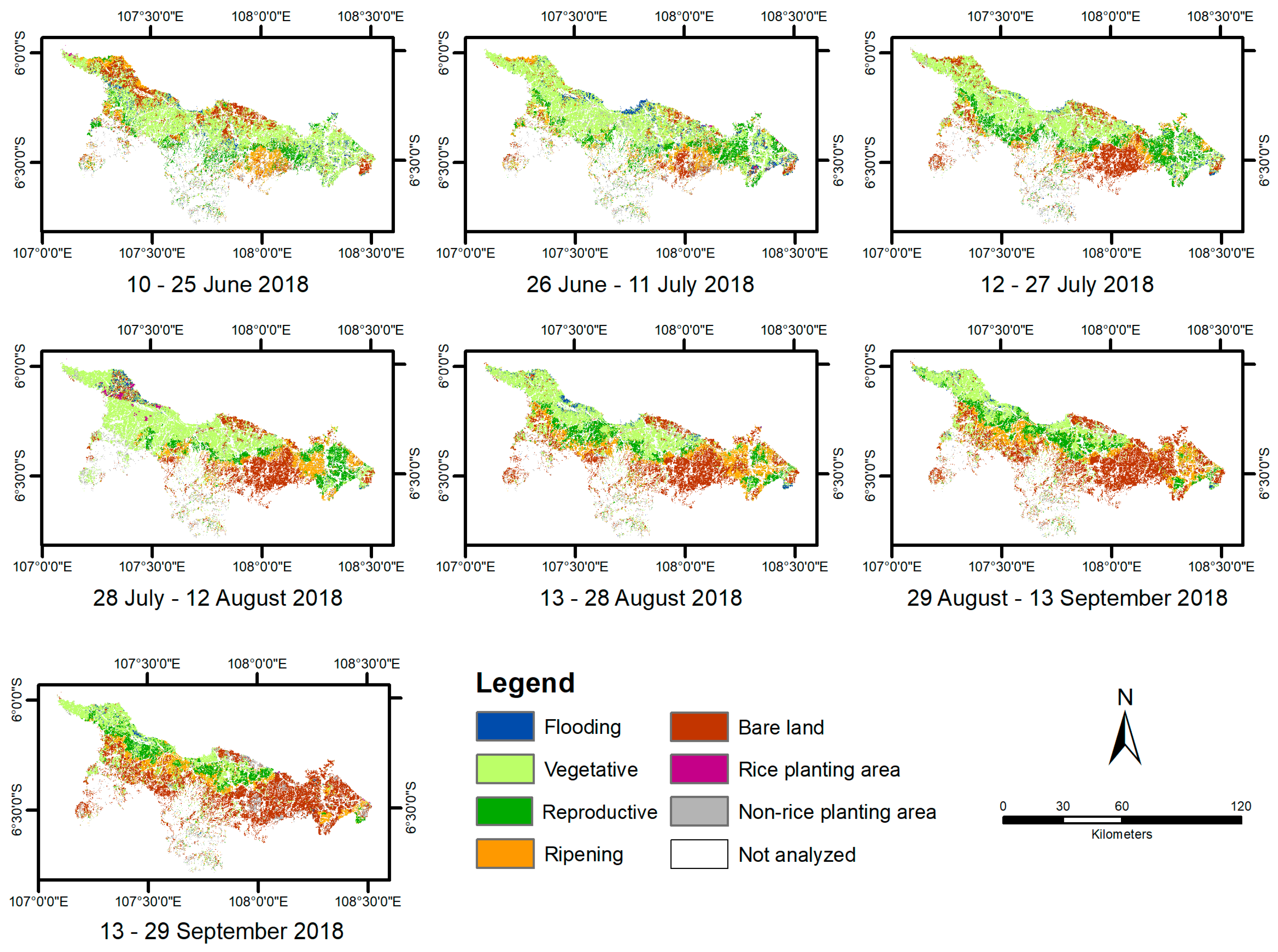
2.2.1. West Area

West Area consists of paddy area in three regencies, which are Karawang (96,482 ha), Subang (84,228 ha), and Indramayu (115,555), with a total area of 310,265 ha [70] (Figure 2). Most of the area is irrigated paddy field from Jatiluhur area (258,633 ha), established on alluvial and lithosol soil. The water distribution is maintained by the state-owned company easing water requirements. However, further issues arise from sedimentation, breaking drainage, and land-use change, especially in the dry season. The season comprises of two rice planting cycles, separated by one month of bare land. This bare land period is intended to rest the soil and stop the crop pest life cycle (Figure S2). The time of planting changes based on the catchment location, with the first planting season starting from November and the second in March in the upper catchment areas. The downstream areas start their season in February due to constant floods during the rainy season, while the second planting is in July.

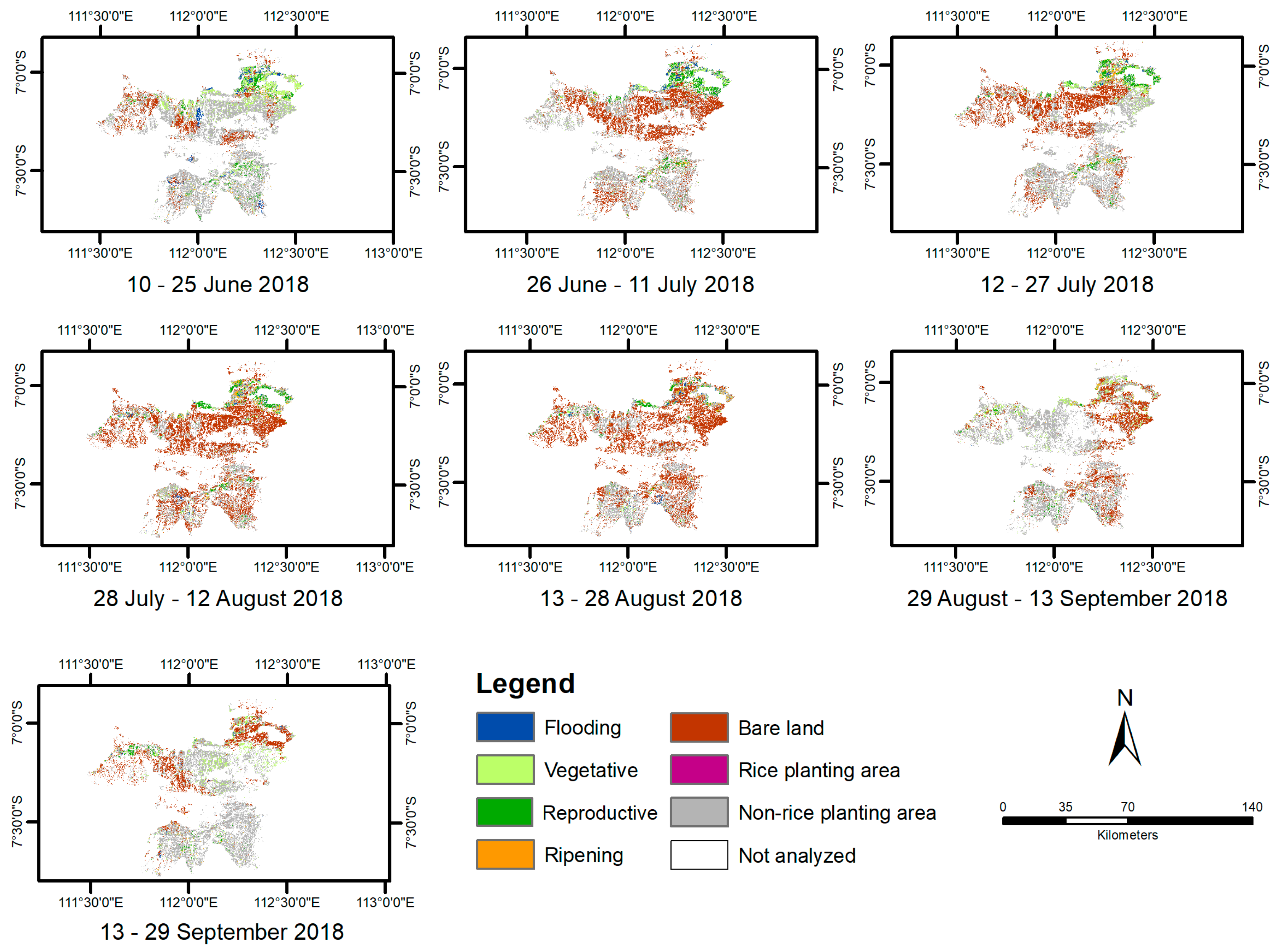
2.2.2. East Area

East Area is located on West Java Province consists of four regencies, including Bojonegoro (78,677 ha), Lamongan (87,336 ha), Jombang (48,704 ha), and Nganjuk (42,918 ha), totalling an area size of 257,635 ha [71] (see Supplementary Table S1). The soil types of this region are much more diverse, including alluvial soils, grumusol, and regosol. The main cropping pattern can be divided into four types. The first cropping pattern is rice planted three times throughout the year with planting times in December, April, and August with water pumping from the Bengawan Solo river for year-round irrigation. This cropping pattern is only found in this one area near the Bengawan Solo river facilitating the farmer to cultivate during the dry season by pumping water. The second cropping pattern is planting rice twice annually with the first planting season in December and the second in April. The third cropping pattern utilises one rice planting period and a secondary crop, such as maize, soybean, and shallots, planted in the dry season. The fourth cropping pattern consists of only rice cultivation during the rainy season (Figure S1).

2.3. Satellite Imagery

This study is based on three satellite datasets from 1 June to 29 September 2018. The first dataset comes from Sentinel-2 A/B in Level-1C (L1C) format, which is a Top-Of-Atmosphere product from Copernicus Open Access Hub [72]. Sentinel-2 satellites provide 5 days of revisited time over the study area. The scenes of Level-1C were subjected to atmospheric corrections into Level-2A by using Sen2Cor [73]. The Sen2Cor produces surface reflectance, which includes seven bands with a 10-m resolution, four bands with a 20-m resolution, six bands with a 60-m resolution, and Scene Land Classification (SCL) with a 20-m resolution. Here, we used 11 bands as the predictors for the Sentinel-2 model (Table S2). Moreover, bands 5, 6, 7, 8A, 11, and 12 were resampled into a 10 × 10 m pixel size to match with high-resolution bands.

The second dataset was MOD13Q1 from Terra sensor with a 250-m resolution from Google Earth Engine (GEE), which was pre-processed to surface reflectance [74,75] and resampled in a 10 × 10 m pixel size. We used this dataset for filling the gap of Sentinel-2 imagery because it is a composite 16-day period of daily MODIS observation. MOD13Q1 consists of the normalized difference vegetation index (NDVI) and enhanced vegetation index (EVI), which are chosen with the highest NDVI value in the 16-day period. The calculation of NDVI and EVI is based on MODIS/Terra bands with the formula as follows:

$$\mathrm{NDVI}=\frac{{\mathsf{\rho }}_{\mathrm{NIR}} {- \mathsf{\rho }}_{\mathrm{Red}}}{{\mathsf{\rho }}_{\mathrm{NIR}}{ + \mathsf{\rho }}_{\mathrm{Red}} },$$

(1)

$$\mathrm{EVI}=2.5 \times \frac{{\mathsf{\rho }}_{\mathrm{NIR}} {- \mathsf{\rho }}_{\mathrm{Red}}}{{\mathsf{\rho }}_{\mathrm{NIR}}{ + 6 \times \mathsf{\rho }}_{\mathrm{Red}} - {7.5 \times \mathsf{\rho }}_{\mathrm{Blue}} +1}.$$

(2)

The third dataset was Sentinel-1A, which was downloaded from GEE and pre-processed with Sentinel-1 toolbox to remove thermal noise, calibrating radiometric and terrain correction (https://developers.google.com/earth-engine/sentinel1). The Sentinel-1 has 12 days of revisited time on the study area due to the location on the equator. We used vertical-horizontal backscattering (VH) descending data and Minimised Interferometric Wide Swath (IW) mode, which consists of vertical-horizontal (VH), vertical-vertical backscattering (VV), and angle bands (Table S2). Thus, the speckle noise of VH values was reduced using the refined-Lee filter with a 7 × 7 window size [55,76,77,78]. This dataset has already been used for mapping the paddy area due to the high sensitivity of water presence in rice cultivation area globally [33,40,41,42,44]. In this study, we used VH as predictors because the VH is more consistent and sensitive in the detection of rice research works than VV backscattering, as suggested in previous works [79,80].

The total number of acquisitions used in this study were 200 scenes for Sentinel-2, 28 scenes for Sentinel-1, and 17 composite scenes for MOD13Q1 (Table S3). All of the dataset was masked with a high-resolution paddy field area from the Indonesia Ministry of Agriculture to reduce complexity with other land use before further processing.

3. Methods

The workflow of analysing multisource remote sensing data for multitemporal mapping of rice growth stages from June–September 2018 was illustrated in Figure 3. First, we labelled and synchronised data from multiple satellites (Sentinel-2, MOD13Q1, and Sentinel-1) with the collected field data. The next step is to build two separate prediction models for rice growth stages using the support vector machine methodology for the Sentinel-2 and another for fusion between MOD13Q1 and Sentinel-1 (MOD13Q1/Sentinel-1). After assessing the accuracy of both models (Sentinel-2 and MOD13Q1/Sentinel-1), the image data were combined into one time series to fill the cloud-obscured pixels of Sentinel-2. Additionally, rice planting detection was applied to separate rice cultivation and non-rice cultivation activity on the rice fields. The final rice growth stages map is the integration of the Sentinel-2/MOD13Q1/Sentinel-1 maps. Finally, we calculated the consistency percentage of the Sentinel-2 and Sentinel-2/MOD13Q1/Sentinel-1 maps over time. In the following subsection, the data conversion steps are described in detail.

3.1. Field Data and Dataset Labelling

The field data was collected as purposive and random sampling with a Global Positioning System (GPS)-enabled mobile phones and synchronised with a pocket GPS receiver between 20 July and 4 September 2018. The sampling points were selected randomly with a 500-m buffer distance using the official paddy area as the base map, which returned 227 points in the West Area and 171 points in the East Area in total. These sites were then visited in the field. The enumerator of the field data made sure that the sampling area has a dimension at least of 50 × 50 m and contained the same rice growth stage throughout to reduce impacts of mixed pixels. Each field site has associated field photos that were used for labelling. The field observations were then matched up with the closest and cloud-free satellite dataset’s date for extraction.

The flooding class has been underrepresented due to fieldwork being conducted in the dry season. To ensure the field dataset was balanced, 70 flooding locations were manually extracted from a Sentinel-2 false colour composite image, taken on 6 June 2018. In total, the number of Sentinel-2 datasets utilised was 426 observations, and MOD13Q1/Sentinel-1 had 468 observations. The difference is due to the changes in cloud cover within the datasets.

3.2. Prediction Models for the Rice Growth Stages

In this study, we used SVM because of its suitability in remote sensing data applications and its capacity to handle complex classification problems [81,82]. SVM maps the data points in high-dimensional feature space and separates the class using hyperplane with a kernel function, such as linear, polynomial, sigmoid, and radial function. The closest data points of the hyperplane become the support vectors, which determine the position and orientation of the hyperplane to find the maximum margin (the distance between the support vectors with the hyperplane) [83]. Here, we used the radial basis function (RBF) because of the high variability and complex predictors for rice condition [33,80]. Moreover, Kavzoglu and Colkesen [84] suggested that SVM with RBF has advantages, such as training pixels being needed less than with other classifiers and flexible with a statistical distribution range in remotely sensed data. Moreover, SVM with RBF has been applied successfully for rice growth stage mapping before and outperformed other classification methods, such as random forest and neural network [24]. There are two kernel parameters of SVM RBF can be used to increase the accuracy, i.e., cost penalty (C) was used to define trade-off between model complexity and error and Sigma for smoothing the vector [85].

Two SVM models were built in this study, using the R programming language with the caret package [86], as follows:

(a)

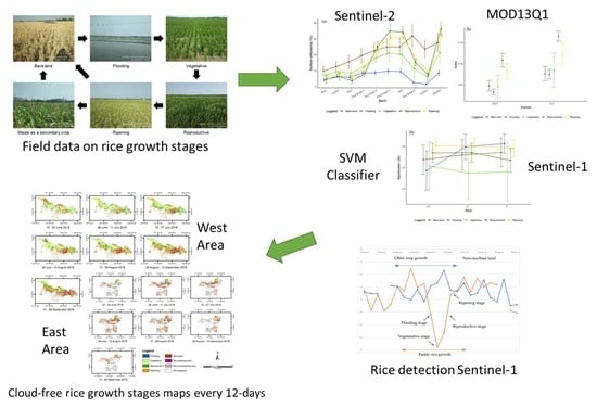
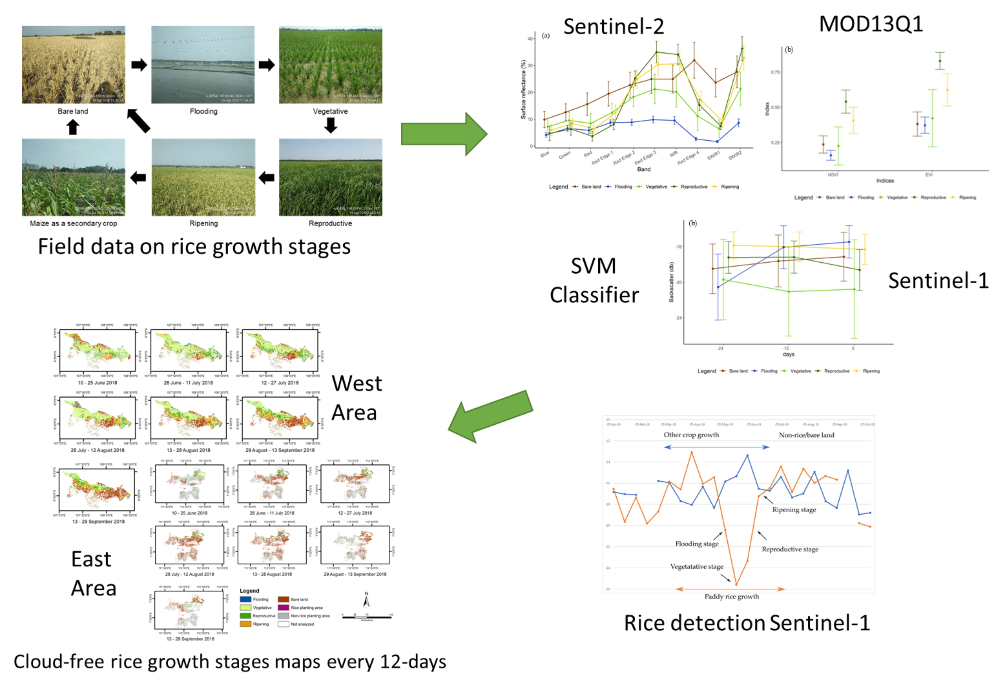
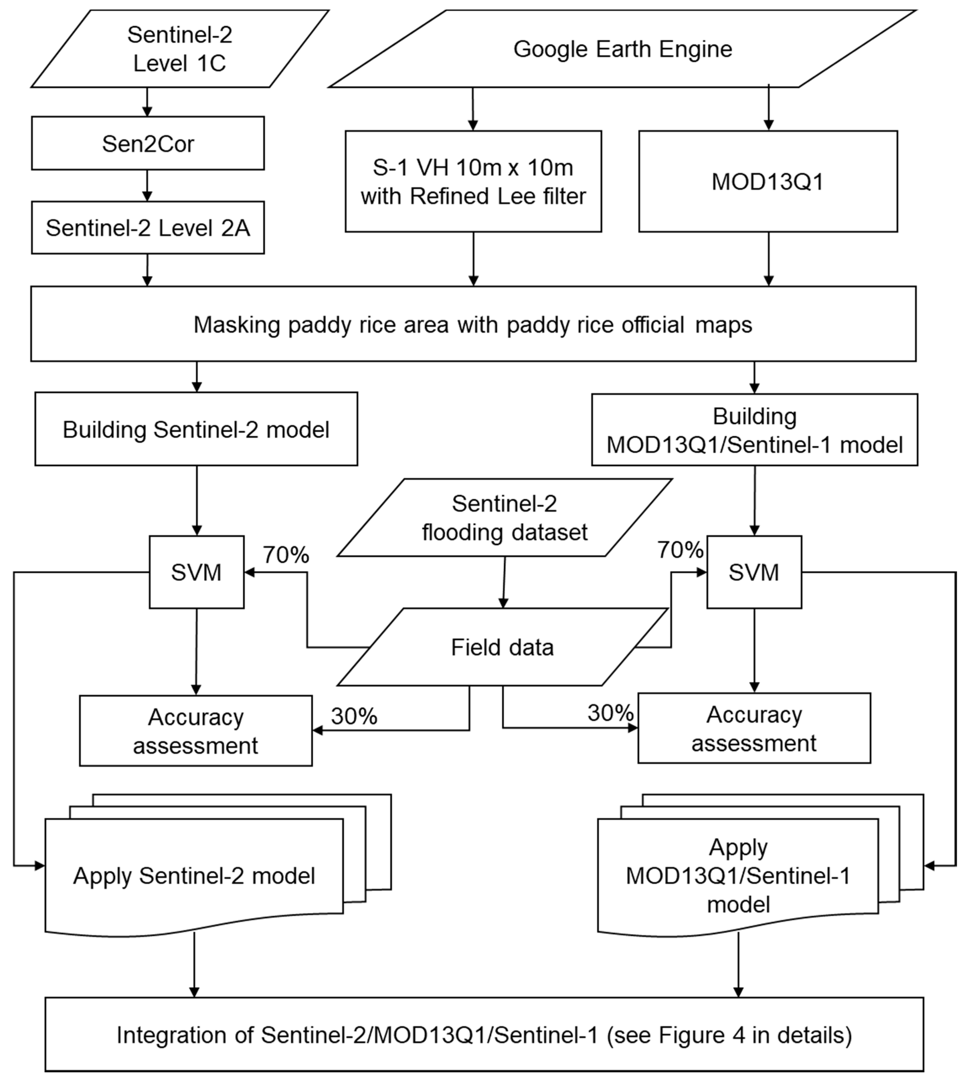
Sentinel-2 model: this prediction model was based on Sentinel-2 input bands (Table S2) as predictors labelled based on the field data temporally closest to the Sentinel-2 imagery acquisition. The Sentinel-2 model to predict rice growth stages was trained using the field dataset with a 70:30% random split (i.e., 299 and 127 observation from the field dataset). The relationship between the bands of Sentinel-2 and the rice growth stages can be expressed as follows:

$$\begin{array}{cc}\hfill Rice growth stages \left(Sentinel2\right)~& B02+B03+B04+B05+B06 +\hfill \\ \hfill & B07+B08+B11+B12+B8A.\hfill \end{array}$$

(3)

(b)

MOD13Q1/Sentinel-1 model was developed by combining MOD13Q1 and Sentinel-1 with predictors of NDVI and EVI from MOD13Q1 and VH for three consecutive three-time lag series (e.g., Sentinel-1 image of VH on t day (T0), t-12 days (T1), and t-24 days (T2) in decibel (dB)). We found that using three consecutive VH values had better accuracy, which can be explained by the typical length of each rice growths stage of around 24 days. We used 330 points for the training dataset and 138 points for the test dataset. The relationship of the MOD13Q1 indices and multitemporal backscattering data of Sentinel-1 and the rice growth stages can be expressed as follows:

$$Rice growth stages \left(MOD13Q1/Sentinel1\right) ~ NDVI+EVI+T0+T1+T2.$$

(4)

The two models were trained with the parameter cost penalty (2ⁿ with n = 1 to 10) to define trade-offs between model complexity and error and Sigma (2⁻²⁵, 2⁻²⁰, 2⁻¹⁵, 2⁻¹⁰, 2⁻⁵, 0) for smoothing the vector [85]. Moreover, the resultant models were cross-validated with the leave-one-out cross-validation method to ensure an unbiased result. The highest accuracy model was selected to be used to classify rice growth stages on the satellite dataset.

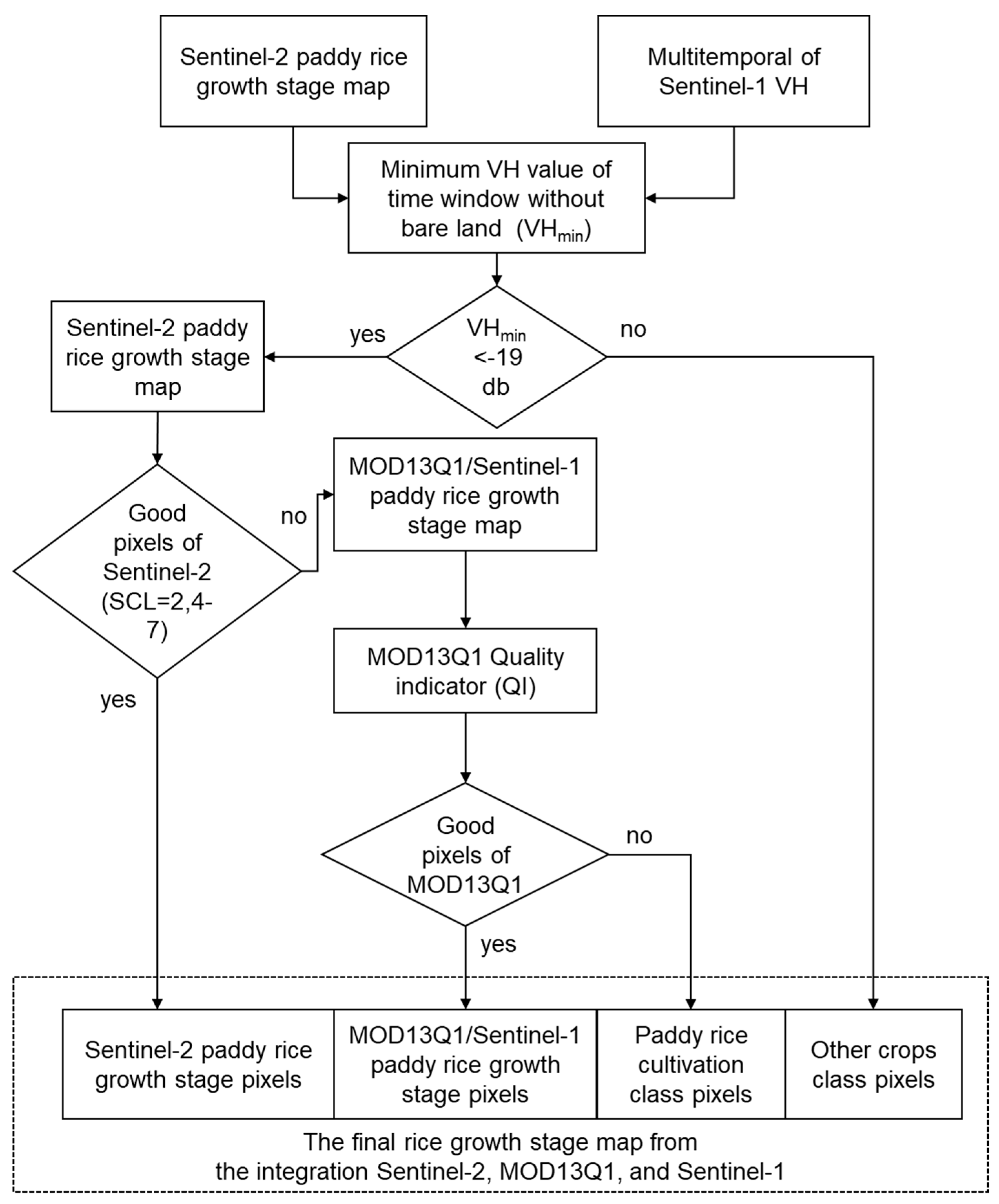
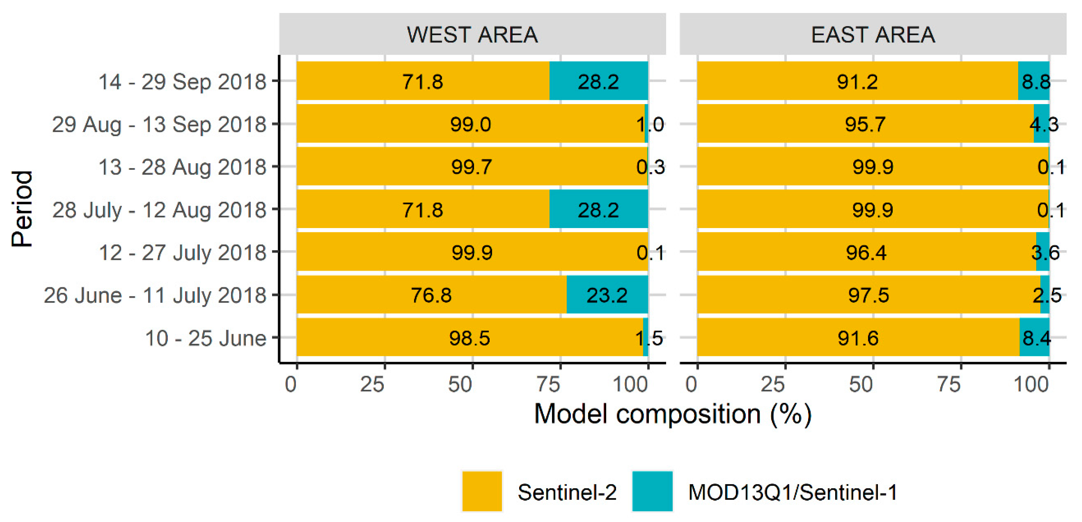
3.3. Generating Multitemporal Maps for Growth Stages by Integrating Sentinel-2/MOD13Q1/Sentinel-1

The final paddy growth stage maps were preferred to be based on Sentinel-2 classification results due to its better resolution than MOD13Q1. However, temporal gaps in the Sentinel-2 data frequently occur due to cloud coverage and shadows. These gaps were filled with the prediction maps generated from the integration of MOD13Q1 and Sentinel-1, which has the same spatial resolution using the resampling technique. The Sentinel-2-based rice growth stage classification was filtered for pixels that had not been bare land for a period 120 days (t₁) and 150 days (t₂) for the East Area and West area, respectively (Figure 4). The timeline of each processing multitemporal map for a 16-day period from 10 June–29 September 2018 can be seen in Table S4.

The differences between time windows were due to different rice cultivation between those areas during the dry season. The East Area has limited time to flood the rice field (<20 days) compared to the West Area (20–40 days). Cloud and shadow were removed using the scene classification band. The Sentinel-1 VH was stacked up to find the lowest VH value (VH_min) over the time window t₁ and t₂ [52]. Low radar backscatter signal can be associated with both the water/vegetative stage due to radar energy reflected off and bare land due to penetration radar energy on dry land [21], making classification using only backscattering sensor data challenging. This confusion can be reduced by utilizing Sentinel-2-based rice growth stage classification. If the VH_min was higher than −19 dB and the rice growth stages are reproductive or ripening, then the pixel value will be replaced by a non-rice planting class, and others would have the rice growth stages value from Sentinel-2 maps. This step is to separate the maize or soybean in the reproductive or ripening phase because the spectral profile is nearly the same as rice’s profile, as illustrated in Figure 5 [21,52].

In some instances, we found even the complete Sentinel-2 and MOD13Q1/Sentinel-1 was unable to have cloud-free data every 16-day period. Thus, we used rice’s detection result to replace the cloud pixels. If the VH_min was lower than −19 dB, the pixel would be marked as the rice planting class. Otherwise, the cloud pixels were marked as another crop class. This resulted in a seven-class map, including bare land, flooding, vegetative, reproductive, ripening, rice planting, and other crops. The integration of Sentinel-2/MOD13Q1/Sentinel-1 will have more rice growth stages data than the Sentinel-2 rice growth stage model alone.

3.4. Accuracy Assessment and Temporal Changes

The accuracy of the Sentinel-2, MOD13Q1/Sentinel-1 model, and rice planting detection were tested using the comparison of predicted values and ground-reference data. By using the confusion matrix, the overall accuracy, user’s accuracy (UA), and producer’s accuracy (PA) can be calculated as suggested by [87,88,89]. The test data for the Sentinel-2 model is 127 points, and MOD13Q1/Sentinel-1 is 138 points.

The temporal changes of predictions maps were reclassified into four classes: (1) No Change, there is no change between stages; (2) change correctly, the stages change into progressively according to the common practices of rice cultivation in Figure 1; (3) change incorrectly, the stages change into two stages forward or back to previous stages; and (4) cloud and shadows, one of the images has cloud/shadows. Thus, the average of no change, change correctly, and change incorrectly can be calculated. The consistency of the map of Sentinel-2 was tested by comparing two images of different 5, 10, 15, 20, 25, and 30 lag-days, and the Sentinel-2 / MOD13Q1 / Sentinel-1 maps were 16-day lag-days, respectively. The formulas of consistency and inconsistency as follows:

$$\mathrm{No} \mathrm{change} (\%)= \frac{{\sum }^{ }\mathrm{Area} \mathrm{of} \mathrm{no} \mathrm{change}}{{\sum }^{ }\mathrm{All} \mathrm{area}}\times 100\%,$$

(5)

$$\mathrm{Change} \mathrm{correctly} (\%)= \frac{{\sum }^{ }\mathrm{Area} \mathrm{of} \mathrm{changed} \mathrm{correctly}}{{\sum }^{ }\mathrm{All} \mathrm{area}}\times 100\%,$$

(6)

$$\mathrm{Consistency} (\%)= \frac{{\sum }^{ }\mathrm{Area} \mathrm{of} \mathrm{no} \mathrm{change}+{\sum }^{ }\mathrm{Area} \mathrm{of} \mathrm{changed} \mathrm{correctly}}{{\sum }^{ }\mathrm{All} \mathrm{area}}\times 100\%,$$

(7)

$$\mathrm{Inconsistency} (\%)= \frac{{\sum }^{ }\mathrm{Area} \mathrm{of} \mathrm{changed} \mathrm{incorrectly}}{{\sum }^{ }\mathrm{All} \mathrm{area}}\times 100\%.$$

(8)

A high consistency value is better since the prediction model can predict the growth stages in current time and previous time accurately.

4. Results

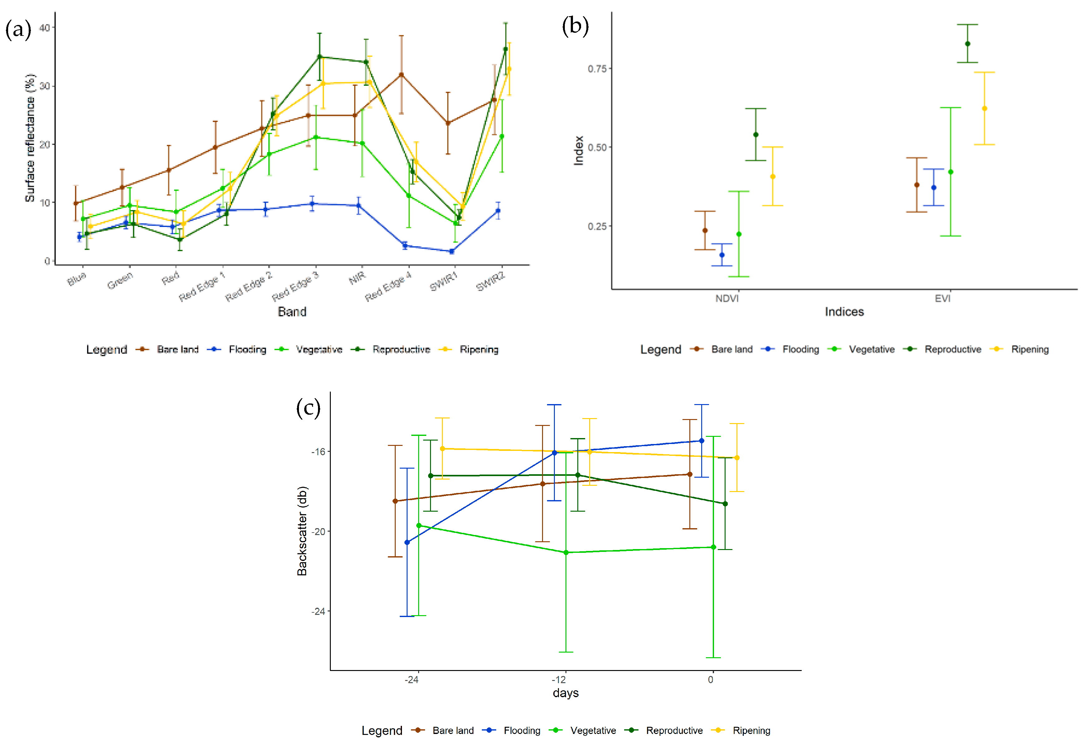
4.1. Spectral Bands

Figure 6a provides the mean and deviation of reflectance values for different rice growth stages based on the ground truth dataset. The result indicates that five classes have distinctive spectral features with significant variability. The reflectance profiles of bare land and flooding are different from rice growth stages (vegetative, reproductive, and ripening) as the rice growth stages have the higher mean value on Red Edge 3, NIR, and SWIR1 band. The flooding class displays the lowest reflection on the NIR band due to almost no reflection off from the vegetation. Moreover, the spectral bands of rice growth stages are concurrent with a multi-angle spectrometer from Sun et al. [87], except for the flooding phase because of the different rice management in the study area. The spectral trend in vegetative and reproductive phases followed a similar pattern.

The averages of NDVI and EVI values can be seen in Figure 6b. It shows that bare land and flooding have similar NDVI values but are different on EVI, which indicated that EVI has a more significant role in separating bare land and flooding [90]. The NDVI and EVI value for rice growth stages follows the common values of rice growth stages where the vegetative stage is the lowest values, and the highest values are the heading stage due to the dense canopy. Lastly, the ripening stage is in the middle as it changes the vegetation to golden colour [91].

Figure 6c shows the relationship between rice growth stages in three consecutive acquisition dates. It shows that the bare land, ripening, and reproductive stages have backscattering values >−19 dB, meaning the surface has relatively dense biomass over 24 days. The bare land is decreasing, and otherwise, ripening and reproductive is decreasing. The main feature is the flooding class, which shows the lowest backscattering value on the previous 24 days and increases afterwards. The backscattering values on the vegetative stage were stable <19 dB, which shows the low scattering due to specular reflection [92].

4.2. Accuracy Assessment of Rice Growth Stages Model

Overall, the accuracy of the Sentinel-2-based model is higher than the combined MOD13Q1/Sentinel-1 model (

Table 1. The confusion matrix performance on the test dataset on Sentinel-2 and MOD13Q1/Sentinel-1.

		Reference Data
	Classes	Bare Land	Flooding	Vegetative	Reproductive	Ripening	Sum	UA (%)
	(a) Sentinel-2
Predicted	Bare land	32	0	0	0	1	33	97.0
data	Flooding	0	21	0	0	0	21	100.0
	Vegetative	1	0	16	0	4	21	76.2
	Reproductive	0	0	0	35	3	40	87.5
	Ripening	0	0	0	1	11	12	91.7
	Sum	33	21	18	36	19	127
	PA (%)	97.0	100.0	88.9	97.2	57.9
	OA (%)	90.6
	(b) MOD13Q1/Sentinel-1
Predicted	Bare land	31	1	5	0	5	42	73.8
data	Flooding	0	18	3	0	0	21	85.7
	Vegetative	2	2	15	0	0	19	78.9
	Reproductive	0	0	3	33	3	39	84.6
	Ripening	4	0	1	1	11	17	64.7
	Sum	37	21	27	34	19	138
	PA (%)	83.8	85.7	55.6	97.1	57.9
	OA (%)	78.3

Note: OA= Overall accuracy, UA = User’s accuracy, and PA = Producer’s accuracy.

). The former can reach a high overall accuracy of 90.6% for all rice growth stages (except ripening) from the producer’s accuracy. The ripening stage is often misclassified with vegetative and reproductive stages. On the other hand, the MOD13Q1/Sentinel-1 model has an overall accuracy of 78.3%, which is lower due to confusion between the ripening class and bare land stage. However, the MOD13Q1/Sentinel-1 model can predict the reproductive stage with a high accuracy (97.1% for PA and 84.6% for UA).

The Sentinel-2 rice growth stage model was able to capture the variation of different rice growth stages, as shown in Figure S2. The map of a particular area on the West Area shows that the vegetative stage was recorded on 1–26 June 2018, followed by the reproductive stage on 1 – 21 July 2018, and then the ripening stage until 10 August 2018. The models show that the land was harvested on 15 August 2018.

Figure S3 shows that the paddy area was surrounded by a non-paddy class as in the East Area, and the irrigation becomes scarce on second rice planting. The vegetative stage was captured on 3–23 June 2018. Then, the reproductive stage was 28 June–23 July 2018. The process of ripening happened between 2 and 17 August 2018. Afterwards, the paddy area becomes bare land or host to other crop types.

4.3. Temporal Changes

The temporal analysis of Sentinel-2 shows that the model was able to capture the change classes with correct ranges of 83.27–90.39% (

Table 2. List of the average of performance from temporal changes analysis of (a) Sentinel-2 and (b) Sentinel-2/MOD13Q1/Sentinel-1.

Time Lag	N	No Change (%)			Change Correctly (%)			Consistency (%)			Inconsistency (%)
	(a) Sentinel-2
		WA	EA	Avg.	WA	EA	Avg.	WA	EA	Avg.	WA	EA	Avg.
5	23	58.72	69.22	63.90	34.00	18.82	26.48	92.72	88.04	90.39	7.28	11.96	9.61
10	22	50.49	68.33	59.35	40.80	18.97	29.96	91.29	87.30	89.31	8.71	12.70	10.69
15	21	44.06	63.41	53.68	46.47	21.86	34.23	90.53	85.27	87.91	9.47	14.73	12.09
20	20	40.57	62.24	51.40	48.79	22.26	35.53	89.36	84.50	86.93	10.64	15.50	13.07
25	19	39.02	55.41	47.22	48.36	26.05	37.21	87.39	81.47	84.43	12.61	18.53	15.57
30	18	35.09	55.77	45.43	50.74	24.92	37.83	85.83	80.70	83.27	14.17	19.30	16.73
	(b) Sentinel-2/MOD13Q1/Sentinel-1
16	6	60.27	65.1	62.64	24.26	18.75	21.50	84.52	83.77	84.15	15.48	16.23	15.85

Note: WA= West Area, EA = East Area, and Avg.=Average.

) of the time. The temporal consistency decreases with the time lag increase. The gradual decrease of the non-change area from 5 to 16 days also confirms that the model can classify the change of rice growth, as shown in Figure 7 and Figure 8. The West Area has a better consistency result since the irrigation schedule is stable, unlike the East Area where irrigation depends on rain.

On the other hand, the temporal analysis of Sentinel-2/MOD13Q1/Sentinel-1 proves that consistency is high (84.15%), which is comparable with the Sentinel-2 consistency on the 15-day period (87.91). Table 2 also indicates that the highest accuracy comes from the East Area, which suggests that the detection of the non-rice planting class is working well. Moreover, Figure 7 and Figure 8 show that final classification images from the integration of the Sentinel-2/MOD13Q1/Sentinel-1 model can deliver a rice growth stage map without cloud and shadows at a 10-m resolution. The Sentinel-2 model was able to fill in >80% of the study area except on 26 June, 28 July, and 14 September 2018 in the West Area (Figure 7). Moreover, the map of the East Area shows that the area of the rice field is dominantly on bare land and non-rice planting except on the area on the north of the East Area, where rice planting can be irrigated with pumping water from the near river (Figure 8).

5. Discussion

5.1. The Performance of Integrating Sentinel-2/MOD13Q1/Sentinel-1 for Mapping Rice Growth Stages

High-resolution multitemporal images of rice growth stages are essential to improve rice production. Although optical images are less favourable for providing continuous images in tropical regions, this research developed a new method to generate multitemporal maps for rice growth stages across Java Island using multisource remote sensing data (Sentinel-2/MOD13Q1/Sentinel-1). This method outperforms a single source of remote sensing information in a real-world application level on rice growth stage mapping as confirmed with previous results, especially to fill the missing data, with an increased overall accuracy 2–5% [64,93,94]. Previous research reported that using single-date data for creating rice maps is not the right strategy for mapping in the long term. These rice growth stage maps showed temporal consistency even without use of the extended temporal composite vegetation index or backscattering profile series. This workflow works best on the paddy area, which is often flat and water covered. The water cover can be picked up by the Sentinel-1 VH signal and improve the temporal frequency of observation, and thus the overall rice growth stage models. Other advantages of this model are that it can be rolled out to cover larger areas (i.e., entire Southeast Asia) with the same farm practices and without depending on a clean time series of the vegetation index.

Increasing the temporal frequency of Sentinel-1 images helped to improve the accuracy of rice growth stages since the backscattering profiles were more accurately determined, particularly on the vegetative stage on the dry season, such as the East Area, where water is scarce. Moreover, Ndikumana et al. [95] reported that Sentinel-1 with a 6-day revisit cycle can produce a rice map with an 88% accuracy in a France rice field, which better compares with the 12-day revisit cycle from the study from Clauss, Ottinger, and Kuenzer [49] with an 83% accuracy.

It is not surprising that the Sentinel-2 based model produced a higher accuracy than the fusion of MOD13Q1 and Sentinel-1 due to the red edge bands with high spatial resolution. These bands can enhance the detection of capturing canopy chlorophyll content better, as suggested by Frampton et al. [96,97], which enables separation of the rice growth stages. The accuracy from the fusion of MOD13Q1 and Sentinel-1 was higher than MODIS information alone, which indicates the complementary information from Sentinel-1. This high accuracy is prominent for the flooding class due to the coarse resolution of the MOD13Q1 data, allowing a more significant portion of mixed pixels to occur compared to the 10-m Sentinel-2 data. The prediction maps from MOD13Q1 and Sentinel-1 were used to fill the missing data or for cloudy pixels of the Sentinel-2.

The consistency of Sentinel-2 has a negative correlation between lag days. The 5-day lag showed the highest consistency percentage and slowly became lower to the 30-day lag-time due to the unchanged stages and correct changes became lower and also became less consistent over the lag days. This result demonstrated that the models could detect the changes in growth stages over time and still have the right consistency (83.27%) over 30 consecutive days. Moreover, the integration of Sentinel-2/MOD13Q1/Sentinel-1 shows an increase the consistency (2.54%) compared with the 5-day lag consistency percentage.

5.2. The Implication of Satellite-Based Monitoring in Tropical Countries

The tropical regions are challenging for optical satellite-based remote sensing due to persistent cloud coverage. Most of the study relies on high-frequency temporal remote sensing data to capture rice growth changes, which are hampered by observation gaps, which can be filled using radar-based imagery (e.g., S1). However, radar-based data also has some limitations, such as geometric distortion and a different response to bare land [98]. Our finding shows that by merging three sensors, we can deliver information on rice growth stages for near real-time monitoring for the Sentinel-2 model, and better accurate information in periodical data for Sentinel-2/MOD13Q1/Sentinel-1 data. Furthermore, this study successfully filled the missing data up to 28.2% in the West Area and 8.8% in the East Area (Figure 9).

Our methodology focuses on developing a groundwork for mapping rice growth stages for near-real-time monitoring, which is challenging to accomplish in an operational level due to the short duration of rice cultivation. Moreover, we focused on making it feasible to incorporate with cloud-based computing or stand-alone workstations and less human interference. Our study is in line with the works of Rudiyanto, et al. [21]. They have succeeded in mapping rice growth stages from multitemporal Sentinel-1 images with unsupervised classification with one month with the same area with cropping pattern information. Significantly, our methodology outperformed the established rice monitoring systems in Indonesia based on MODIS [99] or Landsat rice monitoring [100], as our results created rice growth stage maps at a 10-m spatial resolution with a 16-day period, less cloudy data, and providing present cultivation crop.

Future research should be focused on fusing the multitemporal and multiresolution of satellite observation to increase data availability and accuracy with <100-m spatial resolution. Our study shows that it is possible to fuse the information of the feature level using machine learning. Our experiment showed that the desktop personal computer with 16 GB RAM could classify the image with high speed (17,770 ha/min). This method can also be employed for other remote sensing data, such as PROBA-V or WorldView missions.

This technology implies that the users can compile the information interactively with the user’s interface on a dedicated website or mobile application with less waiting time before the information becomes obsolete. Moreover, the classifier of machine learning can be chosen easily with other open-source machine learning packages, such as TensorFlow [101] with Keras [102] or Scikit-learn [103]. Importantly, the integration of rice growth stages with other information, such as the recommended cropping calendar, climate predictions, weather reports, price trend maps, insurance risk maps, and other in situ knowledge, will improve the rice productivity supporting regional food security.

5.3. Limitation of Satellite Remote Sensing for Rice Mapping

This research has some limitations, such as the availability of cloud-free images. These limitations are further hampered by the fact that there is a bias between the seasons. For example, most optical observations concentrate on the dry season, while only coarser resolution data are available (MODIS and RADAR) on the wet season. Accordingly, some areas with different surface reflectance may be misclassified if it is applied to images in the wet season, such as a wetland. Some traditional farmers switch flooding and drying again, and conduct final flooding before transplanting. This study’s accuracy is highly dependent on the existing rice field map, and, over time, some area could be converted into an urban or industrial area. Long-term rice mapping using multitemporal satellite images has been explored in some studies [33,104,105] with high accuracy, which can be used to correct existing rice field maps every five years.

The East Area has high fragmentation of different crops on the rice field area especially on the north area of Nganjuk regency, which caused problems in classifying between the vegetative stage of rice and shallot cultivation since both crop types need a significant time of water cover to keep the soil moisture. Hence, they are spectrally similar at a specific time, mostly in the early second planting season. Moreover, the fragmented rice field paddocks with an area <0.5 ha made it difficult to be separated automatically in a large area. Thus, additional information is required, including the use of unmanned aerial vehicles (UAVs) [97], ongoing and planned hyperspectral satellite missions (e.g., PRISMA [106] and ENMAP [107]), and webcams [108], for a more apparent separation between such classes.

6. Conclusions

There is a need for timely and accurate spatial information on rice growth stages. This paper has provided an automatic process to build multitemporal maps for rice growth stages with a 10-m spatial resolution, which is sufficient for crop monitoring at the local and national level in developing countries. This information is useful for stakeholders using a combination of Sentinel-2, MOD13Q1, and Sentinel-1 for a near real-time and high accuracy, consistency and temporal frequency (16-day period). Furthermore, the Sentinel-2 model in this study was implemented in Indonesia, with 7.4 million hectares of autonomous data retrieving, analysis, and dissemination, which are available on a website (http://katam.litbang.pertanian.go.id/sc/).

The research presented here is based on open-access satellite data and software, improving its accessibility and uptake by end-users in developing countries. Improving the speed of the mapping process can provide an effective tool for stakeholders and decision-makers to coordinate the distribution of machinery, fertiliser, and water more efficiently. The estimation of rice production can be predicted with better accuracy to control the export and import of rice trade. In addition to the climate change issue, the result is applied as an input of prediction of production and food security in a fragile area, such as drought and flooding, using the temporal analysis or becoming a part of the ASIA Rice project (asia-rice.org) to support the dissemination among its members.

References

- Lowder, S.K.; Skoet, J.; Raney, T. The Number, Size, and Distribution of Farms, Smallholder Farms, and Family Farms Worldwide. World Dev. 2016, 87, 16–29. [Google Scholar] [CrossRef] [Green Version]
- FAOSTAT. Agriculture Database. Available online: http://www.fao.org/indonesia/fao-in-indonesia/indonesia-at-a-glance/en/ (accessed on 15 April 2020).
- Hazaymeh, K.; Hassan, Q.K. A remote sensing-based agricultural drought indicator and its implementation over a semi-arid region, Jordan. J. Arid Land 2017, 9, 319–330. [Google Scholar] [CrossRef]
- Arévalo, P.; Olofsson, P.; Woodcock, C.E. Continuous monitoring of land change activities and post-disturbance dynamics from Landsat time series: A test methodology for REDD+ reporting. Remote Sens. Environ. 2019, 111051. [Google Scholar] [CrossRef]
- Elagouz, M.H.; Abou-Shleel, S.M.; Belal, A.A.; El-Mohandes, M.A.O. Detection of land use/cover change in Egyptian Nile Delta using remote sensing. Egypt. J. Remote Sens. Space Sci. 2019. [Google Scholar] [CrossRef]
- Surmaini, E.; Hadi, T.W.; Subagyono, K.; Puspito, N.T. Early detection of drought impact on rice paddies in Indonesia by means of Niño 3.4 index. Theor. Appl. Climatol. 2015, 121, 669–684. [Google Scholar] [CrossRef]
- Van Ittersum, M.K.; Cassman, K.G.; Grassini, P.; Wolf, J.; Tittonell, P.; Hochman, Z. Yield gap analysis with local to global relevance-A review. Field Crop. Res. 2013, 143, 4–17. [Google Scholar] [CrossRef] [Green Version]
- Guo, B.; Yang, G.; Zhang, F.; Han, F.; Liu, C. Dynamic monitoring of soil erosion in the upper Minjiang catchment using an improved soil loss equation based on remote sensing and geographic information system. Land Degrad. Dev. 2018, 29, 521–533. [Google Scholar] [CrossRef]
- Lewis, D.J.; Barham, B.L.; Zimmerer, K.S. Spatial Externalities in Agriculture: Empirical Analysis, Statistical Identification, and Policy Implications. World Dev. 2008, 36, 1813–1829. [Google Scholar] [CrossRef] [Green Version]
- Raedeke, A.H.; Rikoon, J.S. Temporal and spatial dimensions of knowledge: Implications for sustainable agriculture. Agric. Hum. Values 1997, 14, 145–158. [Google Scholar] [CrossRef]
- Wood, S.; Sebastian, K.; Nachtergaele, F.; Nielsen, D.; Dai, A. Spatial Aspects of the Design and Targeting of Agricultural Development Strategies; IFPRI: Washington, DC, USA, 1999. [Google Scholar]
- Castillo, E.G.; Tuong, T.P.; Singh, U.; Inubushi, K.; Padilla, J. Drought response of dry-seeded rice to water stress timing and N-fertilizer rates and sources. Soil Sci. Plant Nutr. 2006, 52, 496–508. [Google Scholar] [CrossRef]
- Wassmann, R.; Jagadish, S.V.K.; Sumfleth, K.; Pathak, H.; Howell, G.; Ismail, A.; Serraj, R.; Redona, E.; Singh, R.K.; Heuer, S. Regional Vulnerability of Climate Change Impacts on Asian Rice Production and Scope for Adaptation. In Advances in Agronomy; Academic Press: London, UK, 2009; Volume 102, pp. 91–133. [Google Scholar]
- Vermeulen, S.J.; Aggarwal, P.K.; Ainslie, A.; Angelone, C.; Campbell, B.M.; Challinor, A.J.; Hansen, J.W.; Ingram, J.S.I.; Jarvis, A.; Kristjanson, P.; et al. Options for support to agriculture and food security under climate change. Environ. Sci. Policy 2012, 15, 136–144. [Google Scholar] [CrossRef]
- Joshi, N.; Baumann, M.; Ehammer, A.; Fensholt, R.; Grogan, K.; Hostert, P.; Jepsen, M.R.; Kuemmerle, T.; Meyfroidt, P.; Mitchard, E.T.A.; et al. A review of the application of optical and radar remote sensing data fusion to land use mapping and monitoring. Remote Sens. 2016, 8, 70. [Google Scholar] [CrossRef] [Green Version]
- Bruzzone, L. Land Use and Land Cover Mapping in Europe; Springer: London, UK, 2014; Volume 18, pp. 127–143. [Google Scholar] [CrossRef]
- Liu, J.; Zhang, Z.; Xu, X.; Kuang, W.; Zhou, W.; Zhang, S.; Li, R.; Yan, C.; Yu, D.; Wu, S.; et al. Spatial patterns and driving forces of land use change in China during the early 21st century. J. Geogr. Sci. 2010, 20, 483–494. [Google Scholar] [CrossRef]
- Nguyen, T.T.H.; de Bie, C.A.J.M.; Ali, A.; Smaling, E.M.A.; Chu, T.H. Mapping the irrigated rice cropping patterns of the Mekong delta, Vietnam, through hyper-temporal spot NDVI image analysis. Int. J. Remote Sens. 2012, 33, 415–434. [Google Scholar] [CrossRef]
- Sianturi, R.; Jetten, V.G.; Sartohadi, J. Mapping cropping patterns in irrigated rice fields in West Java: Towards mapping vulnerability to flooding using time-series MODIS imageries. Int. J. Appl. Earth Obs. Geoinf. 2018, 66, 1–13. [Google Scholar] [CrossRef]
- Minh, H.V.T.; Avtar, R.; Mohan, G.; Misra, P.; Kurasaki, M. Monitoring and mapping of rice cropping pattern in flooding area in the Vietnamese Mekong delta using Sentinel-1A data: A case of an Giang province. ISPRS Int. J. Geo Inf. 2019, 8, 211. [Google Scholar] [CrossRef] [Green Version]
- Rudiyanto; Minasny, B.; Shah, R.M.; Che Soh, N.; Arif, C.; Indra Setiawan, B. Automated Near-Real-Time Mapping and Monitoring of Rice Extent, Cropping Patterns, and Growth Stages in Southeast Asia Using Sentinel-1 Time Series on a Google Earth Engine Platform. Remote Sens. 2019, 11, 1666. [Google Scholar] [CrossRef] [Green Version]
- Fatikhunnada, A.; Liyantono; Solahudin, M.; Buono, A.; Kato, T.; Seminar, K.B. Assessment of pre-treatment and classification methods for Java paddy field cropping pattern detection on MODIS images. Remote Sens. Appl. Soc. Environ. 2020, 17, 100281. [Google Scholar] [CrossRef]
- Gao, F.; Anderson, M.C.; Zhang, X.; Yang, Z.; Alfieri, J.G.; Kustas, W.P.; Mueller, R.; Johnson, D.M.; Prueger, J.H. Toward mapping crop progress at field scales through fusion of Landsat and MODIS imagery. Remote Sens. Environ. 2017, 188, 9–25. [Google Scholar] [CrossRef] [Green Version]
- Ramadhani, F.; Pullanagari, R.; Kereszturi, G.; Procter, J. Mapping of rice growth phases and bare land using Landsat-8 OLI with machine learning. Int. J. Remote Sens. 2020, 41, 8428–8452. [Google Scholar] [CrossRef]
- Boschetti, M.; Busetto, L.; Manfron, G.; Laborte, A.; Asilo, S.; Pazhanivelan, S.; Nelson, A. PhenoRice: A method for automatic extraction of spatio-temporal information on rice crops using satellite data time series. Remote Sens. Environ. 2017, 194, 347–365. [Google Scholar] [CrossRef] [Green Version]
- Sakamoto, T.; Yokozawa, M.; Toritani, H.; Shibayama, M.; Ishitsuka, N.; Ohno, H. A crop phenology detection method using time-series MODIS data. Remote Sens. Environ. 2005, 96, 366–374. [Google Scholar] [CrossRef]
- Xiao, X.; Boles, S.; Frolking, S.; Li, C.; Babu, J.Y.; Salas, W.; Moore, B., III. Mapping paddy rice agriculture in South and Southeast Asia using multi-temporal MODIS images. Remote Sens. Environ. 2006, 100, 95–113. [Google Scholar] [CrossRef]
- Setiawan, Y.; Rustiadi, E.; Yoshino, K.; Liyantono; Effendi, H. Assessing the Seasonal Dynamics of the Java’s Paddy Field Using MODIS Satellite Images. ISPRS Int. J. Geo Inf. 2014, 3, 110–129. [Google Scholar] [CrossRef] [Green Version]
- Zhang, G.; Xiao, X.; Dong, J.; Kou, W.; Jin, C.; Qin, Y.; Zhou, Y.; Wang, J.; Menarguez, M.A.; Biradar, C. Mapping paddy rice planting areas through time series analysis of MODIS land surface temperature and vegetation index data. ISPRS J. Photogramm. Remote Sens. 2015, 106, 157–171. [Google Scholar] [CrossRef] [Green Version]
- Clauss, K.; Yan, H.; Kuenzer, C. Mapping Paddy Rice in China in 2002, 2005, 2010 and 2014 with MODIS Time Series. Remote Sens. 2016, 8, 434. [Google Scholar] [CrossRef] [Green Version]
- Xiao, X.; Boles, S.; Liu, J.; Zhuang, D.; Frolking, S.; Li, C.; Salas, W.; Moore, B., III. Mapping paddy rice agriculture in southern China using multi-temporal MODIS images. Remote Sens. Environ. 2005, 95, 480–492. [Google Scholar] [CrossRef]
- Sakamoto, T.; Van Nguyen, N.; Ohno, H.; Ishitsuka, N.; Yokozawa, M. Spatio–temporal distribution of rice phenology and cropping systems in the Mekong Delta with special reference to the seasonal water flow of the Mekong and Bassac rivers. Remote Sens. Environ. 2006, 100, 1–16. [Google Scholar] [CrossRef]
- Onojeghuo, A.O.; Blackburn, G.A.; Wang, Q.; Atkinson, P.M.; Kindred, D.; Miao, Y. Mapping paddy rice fields by applying machine learning algorithms to multi-temporal Sentinel-1A and Landsat data. Int. J. Remote Sens. 2018, 39, 1042–1067. [Google Scholar] [CrossRef] [Green Version]
- Kontgis, C.; Schneider, A.; Ozdogan, M. Mapping rice paddy extent and intensification in the Vietnamese Mekong River Delta with dense time stacks of Landsat data. Remote Sens. Environ. 2015, 169, 255–269. [Google Scholar] [CrossRef]
- Campos-Taberner, M.; García-Haro, F.J.; Camps-Valls, G.; Grau-Muedra, G.; Nutini, F.; Crema, A.; Boschetti, M. Multitemporal and multiresolution leaf area index retrieval for operational local rice crop monitoring. Remote Sens. Environ. 2016, 187, 102–118. [Google Scholar] [CrossRef]
- Li, Y.; Liao, Q.; Li, X.; Liao, S.; Chi, G.; Peng, S. Towards an operational system for regional-scale rice yield estimation using a time-series of Radarsat ScanSAR images. Int. J. Remote Sens. 2003, 24, 4207–4220. [Google Scholar] [CrossRef]
- Zhang, Y.; Liu, X.; Su, S.; Wang, C. Retrieving canopy height and density of paddy rice from Radarsat-2 images with a canopy scattering model. Int. J. Appl. Earth Obs. Geoinf. 2014, 28, 170–180. [Google Scholar] [CrossRef]
- Wang, C.; Wu, J.; Zhang, Y.; Pan, G.; Qi, J.; Salas, W.A. Characterizing L-band scattering of paddy rice in southeast china with radiative transfer model and multitemporal ALOS/PALSAR imagery. IEEE Trans. Geosci. Remote Sens. 2009, 47, 988–998. [Google Scholar] [CrossRef]
- Zhang, Y.; Wang, C.; Wu, J.; Qi, J.; Salas, W.A. Mapping paddy rice with multitemporal ALOS/PALSAR imagery in Southeast China. Int. J. Remote Sens. 2009, 30, 6301–6315. [Google Scholar] [CrossRef]
- Mansaray, L.R.; Zhang, D.; Zhou, Z.; Huang, J. Evaluating the potential of temporal Sentinel-1A data for paddy rice discrimination at local scales. Remote Sens. Lett. 2017, 8, 967–976. [Google Scholar] [CrossRef]
- Lasko, K.; Vadrevu, K.P.; Tran, V.T.; Justice, C. Mapping Double and Single Crop Paddy Rice with Sentinel-1A at Varying Spatial Scales and Polarizations in Hanoi, Vietnam. IEEE J. Sel. Top. Appl. Earth Obs. Remote Sens. 2018, 11, 498–512. [Google Scholar] [CrossRef]
- Bazzi, H.; Baghdadi, N.; El Hajj, M.; Zribi, M.; Minh, D.H.T.; Ndikumana, E.; Courault, D.; Belhouchette, H. Mapping paddy rice using Sentinel-1 SAR time series in Camargue, France. Remote Sens. 2019, 11, 887. [Google Scholar] [CrossRef] [Green Version]
- Dirgahayu, D.; Made Parsa, I. Detection Phase Growth of Paddy Crop Using SAR Sentinel-1 Data. IOP Conf. Ser. Earth Environ. Sci. 2019, 280. [Google Scholar] [CrossRef]
- Singha, M.; Dong, J.; Zhang, G.; Xiao, X. High resolution paddy rice maps in cloud-prone Bangladesh and Northeast India using Sentinel-1 data. Sci. Data 2019, 6, 1–10. [Google Scholar] [CrossRef]
- Jo, H.-W.; Lee, S.; Park, E.; Lim, C.-H.; Song, C.; Lee, H.; Ko, Y.; Cha, S.; Yoon, H.; Lee, W.-K. Deep Learning Applications on Multitemporal SAR (Sentinel-1) Image Classification Using Confined Labeled Data: The Case of Detecting Rice Paddy in South Korea. IEEE Trans. Geosci. Remote Sens. 2020, 58, 7589–7601. [Google Scholar] [CrossRef]
- Yin, Q.; Liu, M.; Cheng, J.; Ke, Y.; Chen, X. Mapping paddy rice planting area in northeastern China using spatiotemporal data fusion and phenology-based method. Remote Sens. 2019, 11, 1699. [Google Scholar] [CrossRef] [Green Version]
- Mosleh, M.K.; Hassan, Q.K.; Chowdhury, E.H. Application of remote sensors in mapping rice area and forecasting its production: A review. Sensors 2015, 15, 769–791. [Google Scholar] [CrossRef] [Green Version]
- Gumma, M.K.; Nelson, A.; Thenkabail, P.S.; Singh, A.N. Mapping rice areas of South Asia using MODIS multitemporal data. J. Appl. Remote Sens. 2011, 5. [Google Scholar] [CrossRef] [Green Version]
- Clauss, K.; Ottinger, M.; Kuenzer, C. Mapping rice areas with Sentinel-1 time series and superpixel segmentation. Int. J. Remote Sens. 2018, 39, 1399–1420. [Google Scholar] [CrossRef] [Green Version]
- Chandna, P.K.; Mondal, S. Analyzing multi-year rice-fallow dynamics in Odisha using multi-temporal Landsat-8 OLI and Sentinel-1 Data. GISci. Remote Sens. 2020, 57, 431–449. [Google Scholar] [CrossRef]
- Phung, H.-P.; Nguyen, L.-D.; Nguyen-Huy, T.; Le-Toan, T.; Apan, A. Monitoring rice growth status in the Mekong Delta, Vietnam using multitemporal Sentinel-1 data. J. Appl. Remote Sens. 2020, 14, 014518. [Google Scholar] [CrossRef] [Green Version]
- Liu, Y.; Chen, K.; Xu, P.; Li, Z. Modeling and Characteristics of Microwave Backscattering From Rice Canopy Over Growth Stages. IEEE Trans. Geosci. Remote Sens. 2016, 54, 6757–6770. [Google Scholar] [CrossRef]
- Pham-Duc, B.; Prigent, C.; Aires, F. Surface Water Monitoring within Cambodia and the Vietnamese Mekong Delta over a Year, with Sentinel-1 SAR Observations. Water 2017, 9, 366. [Google Scholar] [CrossRef] [Green Version]
- Ndikumana, E.; Ho Tong Minh, D.; Dang Nguyen, H.T.; Baghdadi, N.; Courault, D.; Hossard, L.; El Moussawi, I. Estimation of Rice Height and Biomass Using Multitemporal SAR Sentinel-1 for Camargue, Southern France. Remote Sens. 2018, 10, 1394. [Google Scholar] [CrossRef] [Green Version]
- Lee, J.S.; Jurkevich, L.; Dewaele, P.; Wambacq, P.; Oosterlinck, A. Speckle filtering of synthetic aperture radar images: A review. Remote Sens. Rev. 1994, 8, 313–340. [Google Scholar] [CrossRef]
- Sica, F.; Gobbi, G.; Rizzoli, P.; Bruzzone, L. ϕ-Net: Deep Residual Learning for InSAR Parameters Estimation. IEEE Trans. Geosci. Remote Sens. 2020, 1–25. [Google Scholar] [CrossRef]
- Kang, J.; Hong, D.; Liu, J.; Baier, G.; Yokoya, N.; Demir, B. Learning Convolutional Sparse Coding on Complex Domain for Interferometric Phase Restoration. IEEE Trans. Neural Netw. Learn. Syst. 2020, 1–15. [Google Scholar] [CrossRef] [Green Version]
- Ding, M.; Guan, Q.; Li, L.; Zhang, H.; Liu, C.; Zhang, L. Phenology-based rice paddy mapping using multi-source satellite imagery and a fusion algorithm applied to the Poyang Lake plain, Southern China. Remote Sens. 2020, 12, 1022. [Google Scholar] [CrossRef] [Green Version]
- Belgiu, M.; Stein, A. Spatiotemporal image fusion in remote sensing. Remote Sens. 2019, 11, 818. [Google Scholar] [CrossRef] [Green Version]
- Ghassemian, H. A review of remote sensing image fusion methods. Inf. Fusion 2016, 32, 75–89. [Google Scholar] [CrossRef]
- Waske, B.; Benediktsson, J.A. Fusion of support vector machines for classification of multisensor data. IEEE Trans. Geosci. Remote Sens. 2007, 45, 3858–3866. [Google Scholar] [CrossRef]
- Schmitt, M.; Zhu, X.X. Data Fusion and Remote Sensing: An ever-growing relationship. IEEE Geosci. Remote Sens. Mag. 2016, 4, 6–23. [Google Scholar] [CrossRef]
- Park, S.; Im, J.; Park, S.; Yoo, C.; Han, H.; Rhee, J. Classification and mapping of paddy rice by combining Landsat and SAR time series data. Remote Sens. 2018, 10, 447. [Google Scholar] [CrossRef] [Green Version]
- Cai, Y.; Lin, H.; Zhang, M. Mapping paddy rice by the object-based random forest method using time series Sentinel-1/Sentinel-2 data. Adv. Space Res. 2019, 64, 2233–2244. [Google Scholar] [CrossRef]
- Inoue, Y.; Kurosu, T.; Maeno, H.; Uratsuka, S.; Kozu, T.; Dabrowska-Zielinska, K.; Qi, J. Season-long daily measurements of multifrequency (Ka, Ku, X, C, and L) and full-polarization backscatter signatures over paddy rice field and their relationship with biological variables. Remote Sens. Environ. 2002, 81, 194–204. [Google Scholar] [CrossRef]
- Fageria, N.K. Yield Physiology of Rice. J. Plant Nutr. 2007, 30, 843–879. [Google Scholar] [CrossRef]
- Hardke, J.T. Arkansas Rice Production Handbook; Misc. Publ.; University of Arkansas Division of Agriculture: Little Rock, AR, USA, 2013; Volume 192. [Google Scholar]
- Bouman, B. Rice Knowledge Bank. Available online: www.knowledgebank.irri.org (accessed on 20 July 2019).
- Kottek, M.; Grieser, J.; Beck, C.; Rudolf, B.; Rubel, F. World map of the Köppen-Geiger climate classification updated. Meteorol. Z. 2006, 15, 259–263. [Google Scholar] [CrossRef]
- BPS-West-Java. West Java Province in Figures 2018; Statistics of West Java Agency: Bandung, West Java, Indonesia, 2018. [Google Scholar]
- BPS-East-Java. East Java Province in Figures 2018; Statistics of East Java Agency: Surabaya, East Java, Indonesia, 2018. [Google Scholar]
- Gascon, F.; Bouzinac, C.; Thépaut, O.; Jung, M.; Francesconi, B.; Louis, J.; Lonjou, V.; Lafrance, B.; Massera, S.; Gaudel-Vacaresse, A.; et al. Copernicus Sentinel-2A Calibration and Products Validation Status. Remote Sens. 2017, 9, 584. [Google Scholar] [CrossRef] [Green Version]
- Louis, J.; Debaecker, V.; Pflug, B.; Main-Knorn, M.; Bieniarz, J.; Mueller-Wilm, U.; Cadau, E.; Gascon, F. SENTINEL-2 SEN2COR: L2A Processor for Users. In Proceedings of the ESA Living Planet Symposium, Prague, Czech Republic, 9–13 May 2016; pp. 1–8. [Google Scholar]
- Sukmono, A. Identification of rice field using Multi-Temporal NDVI and PCA method on Landsat 8 (Case Study: Demak, Central Java). IOP Conf. Ser. Earth Environ. Sci. 2017, 54, 012001. [Google Scholar] [CrossRef]
- Gorelick, N.; Hancher, M.; Dixon, M.; Ilyushchenko, S.; Thau, D.; Moore, R. Google Earth Engine: Planetary-scale geospatial analysis for everyone. Remote Sens. Environ. 2017. [Google Scholar] [CrossRef]
- Lavreniuk, M.; Kussul, N.; Meretsky, M.; Lukin, V.; Abramov, S.; Rubel, O. Impact of SAR data filtering on crop classification accuracy. In Proceedings of the 2017 IEEE First Ukraine Conference on Electrical and Computer Engineering (UKRCON), Kiev, Ukraine, 29 May–2 June 2017; pp. 912–917. [Google Scholar]
- Plank, S.; Jüssi, M.; Martinis, S.; Twele, A. Mapping of flooded vegetation by means of polarimetric Sentinel-1 and ALOS-2/PALSAR-2 imagery. Int. J. Remote Sens. 2017, 38, 3831–3850. [Google Scholar] [CrossRef]
- Lee, J.-S. Refined filtering of image noise using local statistics. Comput. Graph. Image Process. 1981, 15, 380–389. [Google Scholar] [CrossRef]
- Nguyen, D.B.; Gruber, A.; Wagner, W. Mapping rice extent and cropping scheme in the Mekong Delta using Sentinel-1A data. Remote Sens. Lett. 2016, 7, 1209–1218. [Google Scholar] [CrossRef]
- Son, N.-T.; Chen, C.-F.; Chen, C.-R.; Minh, V.-Q. Assessment of Sentinel-1A data for rice crop classification using random forests and support vector machines. Geocarto Int. 2017, 587–601. [Google Scholar] [CrossRef]
- Guyon, I.; Vapnik, V.; Boser, B.; Bottou, L.; Solla, S.A. Capacity control in linear classifiers for pattern recognition. In Proceedings of the 11th IAPR International Conference on Pattern Recognition. Conference B: Pattern Recognition Methodology and Systems, Hague, The Netherlands, 30 August–3 September 1992; Volume 2, pp. 385–388. [Google Scholar]
- Cortes, C.; Vapnik, V. Support-Vector Networks. Mach. Learn. 1995, 20, 273–297. [Google Scholar] [CrossRef]
- Raghavendra, S.; Deka, P.C. Support vector machine applications in the field of hydrology: A review. Appl. Soft Comput. 2014, 19, 372–386. [Google Scholar] [CrossRef]
- Kavzoglu, T.; Colkesen, I. A kernel functions analysis for support vector machines for land cover classification. Int. J. Appl. Earth Obs. Geoinf. 2009, 11, 352–359. [Google Scholar] [CrossRef]
- Mountrakis, G.; Im, J.; Ogole, C. Support vector machines in remote sensing: A review. ISPRS J. Photogramm. Remote Sens. 2011, 66, 247–259. [Google Scholar] [CrossRef]
- Kuhn, M. Building Predictive Models in R Using the caret Package. J. Stat. Softw. 2008, 28, 26. [Google Scholar] [CrossRef] [Green Version]
- Sun, T.; Fang, H.; Liu, W.; Ye, Y. Impact of water background on canopy reflectance anisotropy of a paddy rice field from multi-angle measurements. Agric. For. Meteorol. 2017, 233, 143–152. [Google Scholar] [CrossRef]
- Olofsson, P.; Foody, G.M.; Herold, M.; Stehman, S.V.; Woodcock, C.E.; Wulder, M.A. Good practices for estimating area and assessing accuracy of land change. Remote Sens. Environ. 2014, 148, 42–57. [Google Scholar] [CrossRef]
- Foody, G.M. Status of land cover classification accuracy assessment. Remote Sens. Environ. 2002, 80, 185–201. [Google Scholar] [CrossRef]
- Xiao, X.; Braswell, B.; Zhang, Q.; Boles, S.; Frolking, S.; Moore Iii, B. Sensitivity of vegetation indices to atmospheric aerosols: Continental-scale observations in Northern Asia. Remote Sens. Environ. 2003, 84, 385–392. [Google Scholar] [CrossRef]
- Qiu, B.; Zhong, M.; Tang, Z.; Wang, C. A new methodology to map double-cropping croplands based on continuous wavelet transform. Int. J. Appl. Earth Obs. Geoinf. 2014, 26, 97–104. [Google Scholar] [CrossRef]
- Hoang, H.K.; Bernier, M.; Duchesne, S.; Tran, Y.M. Rice Mapping Using RADARSAT-2 Dual- and Quad-Pol Data in a Complex Land-Use Watershed: Cau River Basin (Vietnam). IEEE J. Sel. Top. Appl. Earth Obs. Remote Sens. 2016, 9, 3082–3096. [Google Scholar] [CrossRef] [Green Version]
- Orynbaikyzy, A.; Gessner, U.; Conrad, C. Crop type classification using a combination of optical and radar remote sensing data: A review. Int. J. Remote Sens. 2019, 40, 6553–6595. [Google Scholar] [CrossRef]
- Lopes, M.; Frison, P.-L.; Crowson, M.; Warren-Thomas, E.; Hariyadi, B.; Kartika, W.D.; Agus, F.; Hamer, K.C.; Stringer, L.; Hill, J.K.; et al. Improving the accuracy of land cover classification in cloud persistent areas using optical and radar satellite image time series. Methods Ecol. Evol. 2020, 11, 532–541. [Google Scholar] [CrossRef]
- Ndikumana, E.; Ho Tong Minh, D.; Baghdadi, N.; Courault, D.; Hossard, L. Deep Recurrent Neural Network for Agricultural Classification using multitemporal SAR Sentinel-1 for Camargue, France. Remote Sens. 2018, 10, 1217. [Google Scholar] [CrossRef] [Green Version]
- Frampton, W.J.; Dash, J.; Watmough, G.; Milton, E.J. Evaluating the capabilities of Sentinel-2 for quantitative estimation of biophysical variables in vegetation. ISPRS J. Photogramm. Remote Sens. 2013, 82, 83–92. [Google Scholar] [CrossRef] [Green Version]
- Zhou, X.; Zheng, H.B.; Xu, X.Q.; He, J.Y.; Ge, X.K.; Yao, X.; Cheng, T.; Zhu, Y.; Cao, W.X.; Tian, Y.C. Predicting grain yield in rice using multi-temporal vegetation indices from UAV-based multispectral and digital imagery. ISPRS J. Photogramm. Remote Sens. 2017, 130, 246–255. [Google Scholar] [CrossRef]
- Perbet, P.; Fortin, M.; Ville, A.; Béland, M. Near real-time deforestation detection in Malaysia and Indonesia using change vector analysis with three sensors. Int. J. Remote Sens. 2019, 40, 7439–7458. [Google Scholar] [CrossRef]
- LAPAN. Rice Growth Stages with Terra MODIS. Available online: http://sipandora.lapan.go.id/site/fasepertumbuhanpadi (accessed on 25 February 2019). (In Indonesian).
- PUSDATIN. Manual of SIMOTANDI Application. Available online: http://sig.pertanian.go.id/pdf/Pedoman_Pemanfaatan_Aplikasi%20_Simotandi.pdf (accessed on 28 March 2019). (In Indonesian).
- Abadi, M.; Barham, P.; Chen, J.; Chen, Z.; Davis, A.; Dean, J.; Devin, M.; Ghemawat, S.; Irving, G.; Isard, M. Tensorflow: A system for large-scale machine learning. In Proceedings of the 12th {USENIX} symposium on operating systems design and implementation ({OSDI} 16), Savannah, GA, USA, 2–4 November 2016; pp. 265–283. [Google Scholar]
- Ketkar, N. Introduction to keras. In Deep Learning with Python; Springer: Berlin, Germany, 2017; pp. 97–111. [Google Scholar]
- Pedregosa, F.; Varoquaux, G.; Gramfort, A.; Michel, V.; Thirion, B.; Grisel, O.; Blondel, M.; Prettenhofer, P.; Weiss, R.; Dubourg, V. Scikit-learn: Machine learning in Python. J. Mach. Learn. Res. 2011, 12, 2825–2830. [Google Scholar]
- Zhou, Y.; Xiao, X.; Qin, Y.; Dong, J.; Zhang, G.; Kou, W.; Jin, C.; Wang, J.; Li, X. Mapping paddy rice planting area in rice-wetland coexistent areas through analysis of Landsat 8 OLI and MODIS images. Int. J. Appl. Earth Obs. Geoinf. 2016, 46, 1–12. [Google Scholar] [CrossRef] [Green Version]
- Dong, J.; Xiao, X.; Menarguez, M.A.; Zhang, G.; Qin, Y.; Thau, D.; Biradar, C.; Moore, B., III. Mapping paddy rice planting area in northeastern Asia with Landsat 8 images, phenology-based algorithm and Google Earth Engine. Remote Sens. Environ. 2016, 185, 142–154. [Google Scholar] [CrossRef] [PubMed] [Green Version]
- Pignatti, S.; Palombo, A.; Pascucci, S.; Romano, F.; Santini, F.; Simoniello, T.; Umberto, A.; Vincenzo, C.; Acito, N.; Diani, M.; et al. The PRISMA hyperspectral mission: Science activities and opportunities for agriculture and land monitoring. In Proceedings of the 2013 IEEE International Geoscience and Remote Sensing Symposium—IGARSS, Melbourne, VIC, Australia, 21–26 July 2013; pp. 4558–4561. [Google Scholar]
- Richter, K.; Hank, T.; Atzberger, C.; Locherer, M.; Mauser, W. Regularization strategies for agricultural monitoring: The EnMAP vegetation analyzer (AVA). In Proceedings of the 2012 IEEE International Geoscience and Remote Sensing Symposium, Munich, Germany, 22–27 July 2012; pp. 6613–6616. [Google Scholar]
- Lebourgeois, V.; Bégué, A.; Labbé, S.; Mallavan, B.; Prévot, L.; Roux, B. Can Commercial Digital Cameras Be Used as Multispectral Sensors? A Crop Monitoring Test. Sensors 2008, 8, 7300–7322. [Google Scholar] [CrossRef]