Validation of Satellite Sea Surface Temperatures and Long-Term Trends in Korean Coastal Regions over Past Decades (1982–2018)


1
Department of Earth Science Education, Seoul National University, Seoul 08826, Korea
2
Research Institute of Oceanography, Seoul National University, Seoul 08826, Korea
*
Author to whom correspondence should be addressed.
Remote Sens. 2020, 12(22), 3742; https://0-doi-org.brum.beds.ac.uk/10.3390/rs12223742
Submission received: 5 October 2020
/
Revised: 11 November 2020
/
Accepted: 12 November 2020
/
Published: 13 November 2020
(This article belongs to the Special Issue Remote Sensing Data Sets)
Abstract
:Validation of daily Optimum Interpolation Sea Surface Temperature (OISST) data from 1982 to 2018 was performed by comparison with quality-controlled in situ water temperature data from Korea Meteorological Administration moored buoys and Korea Oceanographic Data Center observations in the coastal regions around the Korean Peninsula. In contrast to the relatively high accuracy of the SSTs in the open ocean, the SSTs of the coastal regions exhibited large root-mean-square errors (RMSE) ranging from 0.75 K to 1.99 K and a bias ranging from −0.51 K to 1.27 K, which tended to be amplified towards the coastal lines. The coastal SSTs in the Yellow Sea presented much higher RMSE and bias due to the appearance of cold water on the surface induced by vigorous tidal mixing over shallow bathymetry. The long-term trends of OISSTs were also compared with those of in situ water temperatures over decades. Although the trends of OISSTs deviated from those of in situ temperatures in coastal regions, the spatial patterns of the OISST trends revealed a similar structure to those of in situ temperature trends. The trends of SSTs using satellite data explained about 99% of the trends in in situ temperatures in offshore regions (>25 km from the shoreline). This study discusses the limitations and potential of global SSTs as well as long-term SST trends, especially in Korean coastal regions, considering diverse applications of satellite SSTs and increasing vulnerability to climate change.
1. Introduction
The sea surface temperature (SST) is one of the most important variables for monitoring changes in oceanic environments and understanding their link to climate change [1,2]. Satellite-observed SSTs of global oceans as well as local seas have long been validated using various types of temperature measurements from surface drifters, Array for Real-time Geostrophic Oceanography (ARGO), ship-of-opportunity data using Conductivity, Temperature, and Depth (CTD), thermometers, and thermosalinographs (e.g., [3,4,5,6,7,8,9,10,11,12,13,14,15,16,17,18,19]). In the global ocean and local seas, satellite SSTs have been reported to have comparatively good accuracies of approximately 0.5–0.7 K for several retrieval algorithms for infrared sensors (e.g., National Oceanic and Atmospheric Administration/Advanced Very High Resolution Radiometer (NOAA/AVHRR), GMS/S-VISSR (Geostationary Meteorological Satellite/Stretched-Visible Infrared Spin Scan Radiometer), and Along-Track Scanning Radiometer (ATSR) and AVHRR) and microwave sensors (e.g., Tropical Rainfall Measuring Mission/Microwave Imager (TRMM/TMI)) [3,4,5,6,7,8,9,10,11,16,19,20].
Relatively better accuracies of satellite SSTs in the global ocean do not necessarily support the high confidence in the global SSTs in the coastal region of the marginal seas. Comparison studies have revealed relatively low accuracies in coastal areas. The validation results of AVHRR SSTs in three coastal regions of the USA (Gulf of Mexico, Southeast USA, and Northeast USA) showed that the standard deviation was approximately 1.0 °C [21]. Large bias values of up to 6 K between satellite-derived and in situ climatological temperatures were detected in the coastal region of South Africa [22]. The validation of Moderate Resolution Imaging Spectroradiometer (MODIS) SSTs with observations in shallow waters in Florida Bay showed root-mean-square errors (RMSE) and standard deviations higher than 1.5 K [23]. The RMSE of AVHRR SSTs at the coastline ranged from 1.0 K to 2.0 K depending on the temporal difference of the matchup data in the coastal waters of the UK and Ireland [24]. In Korean coastal regions, global SST products showed relatively large RMSE values of over 1.27 K and warm bias over 0.31 K [25], and high-resolution Landsat-8 SSTs had relatively small RMSE values from 0.59 to 0.72 K, as compared with coastal buoy temperatures [26].
Most previous studies have presented lower accuracies of SSTs in the coastal regions than in offshore regions. The SSTs in coastal regions have become increasingly important for understanding air–sea interactions, physical processes, the local ecosystem and biodiversity, coastal disasters, fisheries, and long-term climate change. Therefore, it is crucial to understand the accuracy of satellite SSTs in coastal regions [25,27]. Since the validation procedure of SSTs can provide a means of understanding the coastal processes and applications, the evaluation of the SST accuracies should be performed in coastal zones as much as possible.
In addition to the accuracy of the SSTs, long-term trends of the SSTs are also important, but identifying these trends in coastal waters can be difficult. According to a number of previous studies using various SST databases, it is known that the global-averaged SST has generally increased over the past several decades. The trends of the surface layers within 75 m in the global ocean increased by a total of 4 °C at a rate of 0.11 °C decade−1 between 1971 and 2010, and would have exhibited warming before 1870–1971 [28]. Recently, the SST trends since 1998 showed an opposite change called “global warming hiatus,” a slowdown pattern of the previous global warming (e.g., [29,30,31,32,33]). The estimated SST trends have different results between the composite SST data depending on the period [34,35]. No clear trend was found in Florida Bay when examining AVHRR SST from 1981 to 2016; however, the maximum temperatures increased by 1 °C during this period [23]. In the open ocean, the trends are expected to be more consistent than those in the coastal regions. Accordingly, it is necessary to compare the satellite-based temperature trends with in situ temperature trends in the coastal regions of local seas over the past few decades.
According to [36], a study that analyzed the net SST changes in global coastal regions using data from the United Kingdom Meteorological Office Hadley Center SST climatology [37,38], the rapid warming in 1982–2006 was confined to the Subarctic Gyre, European Seas, and East Asian Seas. These local seas warmed at rates of two to four times the global mean rate. The most rapid warming was observed in the land-locked or semi-enclosed European and East Asian Seas (Baltic Sea, North Sea, Black Sea, East/Japan Sea (EJS), and East China Sea) and also over the Newfoundland–Labrador Shelf. Efforts to monitor SST changes that appear differently according to coastal characteristics are being made, such as the California Cooperative Oceanic Fisheries Investigations (CalCOFI) off the coast of California [39].
The seas around the Korean Peninsula provide a suitable environment to verify the SST trends because of the many buoys and regular measurements at fixed coastal stations (Figure 1b). Such marginal seas and coastal areas are not only affected by the continents surrounding Korea, Japan, and China, but also by the Pacific Ocean. There are rapid changes in the water temperature associated with global warming [40,41,42,43,44,45]. In particular, it is known that coastal areas undergo relatively greater changes. These changes have been monitored through observational data from the buoy systems of the Korea Meteorological Administration (KMA) and the Korea Oceanographic Data Center (KODC) stations that have been managed since the 1960s. Thus, these in situ measurements can be used to investigate the accuracy of satellite-based temperature trends in the seas around Korea over a long period.
Therefore, the objectives of this study are: (1) to compare Optimum Interpolation Sea Surface Temperature (OISST) data with the KMA buoy observation data to analyze the SST accuracy in the coastal region; (2) to compare the KODC ship observation temperature data to analyze the SST accuracy in the offshore and near-coast regions; (3) to evaluate SST trends from the OISST and KODC observation data and to understand the characteristics of the SST trends over decades; and (4) to address the importance of accurate SSTs in coastal regions.
2. Data
2.1. Satellite Sea Surface Temperature
The daily OISST data provided by the NOAA/Earth System Laboratory (ESRL)/Physical Science Division (PSD) are some of the most representative SST databases based on NOAA/AVHRR data the longest period from 1981 onwards. The databases have been developed in the form of weekly OISST version 1 [47], daily OISST version 1 [48], and daily OISST version 2 [49]. The latest version of the database using AVHRR data has only been produced with a temporal resolution of one day and a spatial resolution of 0.25° for the longest period, from August 1981 to the present day. One of the other OISST databases has been produced by combining the AVHRR and AMSR-E data for the decade from 2002 to 2011. Recently, a new version of the daily OISST (version 2.1) from 1 April 2020 has been produced [50].
Considering the characteristics of the OISST database, the daily version 2 high-resolution OISST product was selected to estimate the accuracy of the OISSTs. In addition, OISSTs were utilized to investigate the long-term SST trends for comparison with the trends of in situ temperatures. Since the OISST data using AVHRR data have the longest period, they are the most appropriate to represent the long-term trend. Accordingly, a comparative verification procedure of the OISSTs was performed using all available in situ data temperature measurements from the coastal regions around the Korean Peninsula.
2.2. In Situ Temperature
2.2.1. Buoy Temperature Data
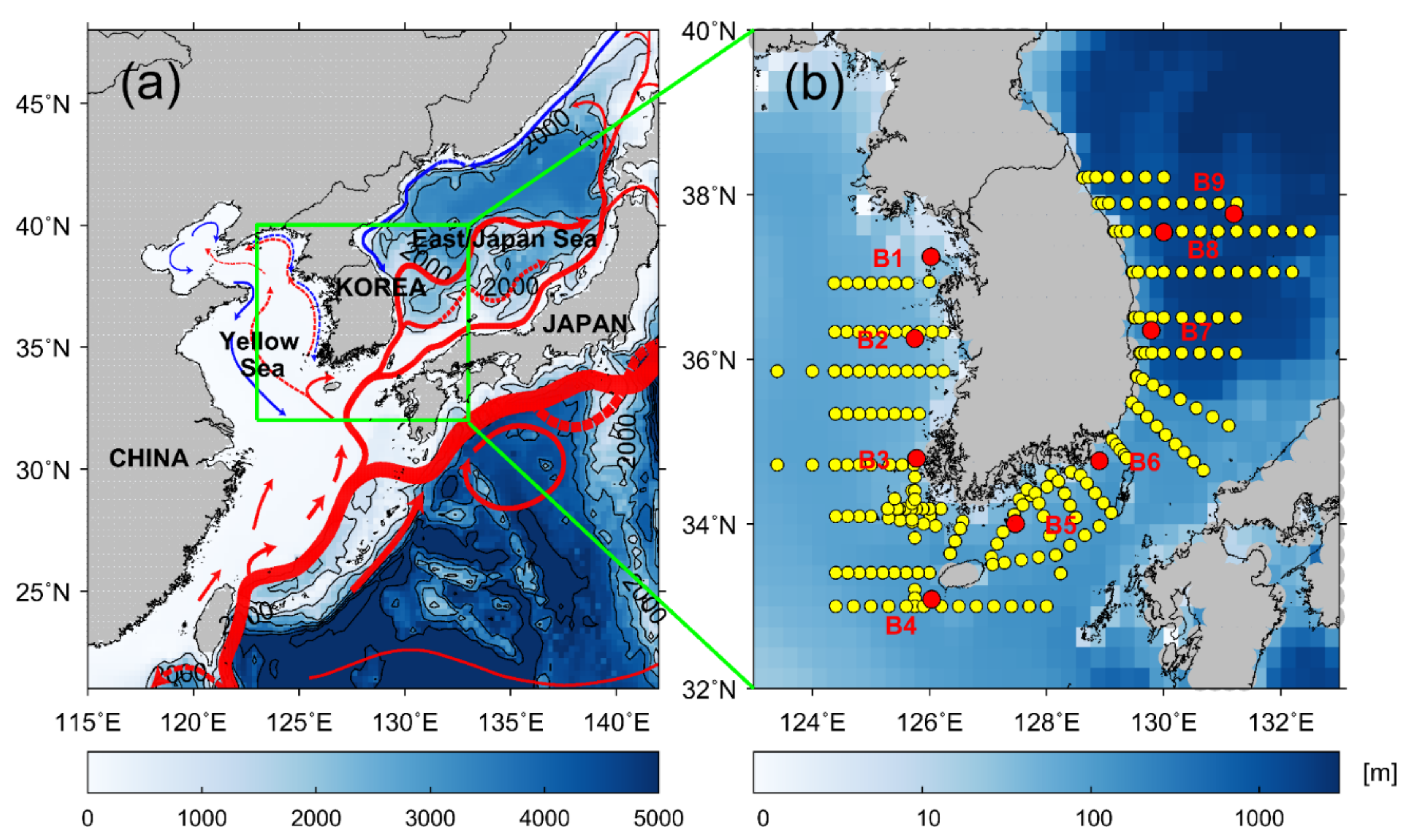
Several meteorological buoys of the KMA have been operating in the seas around the Korean Peninsula since 1996. Considering the operating period of each buoy station, we performed a validation using temperatures of nine KMA buoys, Deokjeokdo (hereafter, B1), Oeyeondo (B2), Chilbaldo (B3), Marado (B4), Geomundo (B5), Geojedo (B6), Pohang (B7), Donghae (B8), and Ulleungdo (B9), as shown by the red circles in Figure 1b.
Table 1 shows detailed information of the KMA buoys in the Yellow Sea (YS) (B1 to B3), in the southern region (B4 to B6), and in the EJS (B7 to B9). Most of the temperature sensors of the buoys are located 0.2 m below the sea surface, with the exception of four buoys (B4, B8, and B9) at 0.4 m. The water depths of the stations vary from 30 m (B1) in the YS to 2200 m (B9) in the EJS. The starting dates of the buoy observations vary from July 1996 (B1) to December 2011 (B9). The buoy stations are located 0.95–84.19 km away from the shoreline of the Korean Peninsula. To proceed with the verification, an accuracy assessment was performed for each station for the entire period from the beginning of the temperature measurements to the end of 2018.
2.2.2. KODC Observation Data
In addition to the KMA buoy data, oceanographic data are also being collected using CTD. From 1961 to the present, the National Institute of Fisheries Science (NIFS) has produced the KODC database by surveying oceanic environments, including sea water temperatures in the seas around the Korean Peninsula, approximately six times a year (during even months). There are many observation stations, including 58, 52, and 54 fixed observation sites in the EJS, YS, and SS, respectively, as marked by the yellow dots in Figure 1b. Temperature as well as other oceanic variables (salinity, dissolved oxygen, and nutrient concentrations (nitrate, phosphate, and silicate)) have been measured and reported at standard observation depths (0, 10, 20, 30, 50, 75, 100, 125, 150, 200, 250, 300, 400, and 500 m) since 1961. We used the 0-m temperature data; however, the temperature was measured at approximately 2–3 m below the sea surface. Since the KODC data include not only offshore regions but also near-coast regions, as shown in Figure 1b, the characteristics of the SST differences as a distance from the coast can be investigated by following each observation line in the YS, the EJS, and the southern coastal regions.
3. Methods
3.1. Quality Control (QC) Procedure for Buoy Data
For the comparison of OISSTs with the KMA buoy data, a series of QC procedures were applied to eliminate abnormal buoy temperature data [25]. The main procedure was composed of limitations on data numbers and the removal of temporal inhomogeneity. First, if the number of temperature measurements was fewer than 10 per day, all observations from that date were removed. A range of diurnal variations were accounted for by removing the same temperatures without any change for 24 h and highly variable temperatures of more than 4 K per day. In addition, the observation data that deviated by three standard deviations (STD) or more from the daily mean were removed. When the STD of the four-day observation temperatures was 0 or more than 2 K, all the data from this period were also excluded from the next procedure.
3.2. Matchup Procedure and Validation
In a matchup procedure between satellite SSTs and in situ temperatures, the temperatures of the KMA buoys were averaged each day to make a matchup database with daily OISSTs. The spatial limit between OISST and the location of the buoys was attributed to the spatial resolution (0.25°) of the OISST database. In the KODC stations, the collocation data were taken with the OISSTs on the same date as the CTD measurements within a distance of 0.25°. The KMA buoys are located 0.95 to 84.19 km from the coastline. The KODC stations are distributed over a wider range of distances from the coastlines from 1.22 km to 145.80 km. The longest distance amounted to 145.80 km in the EJS. In this study, KODC observation stations were divided into “near-coastal” (<25 km) and “offshore” regions (>25 km) based on the distance from land.
The results of the validation of the OISST data using in situ data are presented as fundamental statistical values such as RMSE and bias, as follows:
where is the satellite SST, is the in situ temperature, and is the number of the matchup data between the satellite SSTs and the in situ temperatures.
3.3. Estimation of Temporal Trend
The KODC observation data were measured bimonthly (in even months) over a long time since 1960. Due to occasional severe sea states, the observation dates at each station are not necessarily constant but vary slightly. Although efforts were made to keep the date, the CTD measurements have a temporal range from each given date in even months or later observations in odd months depending on the sea status. Instead of a time-based interpolation of the KODC data, the model in [51] was applied to obtain the rate of changes in water temperatures at once. A time series of SSTs at each station contains diverse variations at frequencies corresponding to short-term, intraseasonal, seasonal, year-to-year variations, and long-term variations over decades. To calculate the long-term trends of SST, we used the model suggested by [51,52] instead of applying a filter (e.g., Trenberth filter [53]) to remove short-term and interannual variations.
The model assumed that the SST at time t is a combination of a constant term (), harmonic constituents with coefficients (, ) at four frequencies from one to four cycles per year (St), a linear trend rate () (°C year−1), and the principal component (PCt) of the empirical orthogonal function (EOF) multiplied by a constant (), where the function represents the strength of El Niño [51].
As the seas around the Korean Peninsula are more affected by the Arctic Oscillation (AO) than by El Niño in winter [54], this study modified Equation (1) by adding a term associated with the AO as follows:
where is the rate of temperature change (°C year−1), is the period of harmonic constituents, and and are the coefficients associated with the El Niño/Southern Oscillation (ENSO) index () and the AO index (), respectively. We used a time series of the Multivariate ENSO Index (MEI) index from 1982 to 2018 as one of the representative ENSO indices (https://www.psl.noaa.gov/enso/mei/). Similarly, the trend of satellite SSTs () at each grid was obtained using Equations (3) and (4). The statistical significance of each trend was tested within a 95% confidence level using the Mann‒Kendall test [55,56].
4. Results
4.1. Comparison of SSTs and Buoy Temperatures
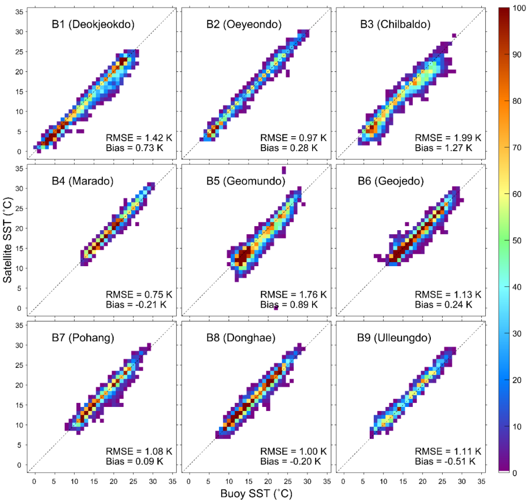
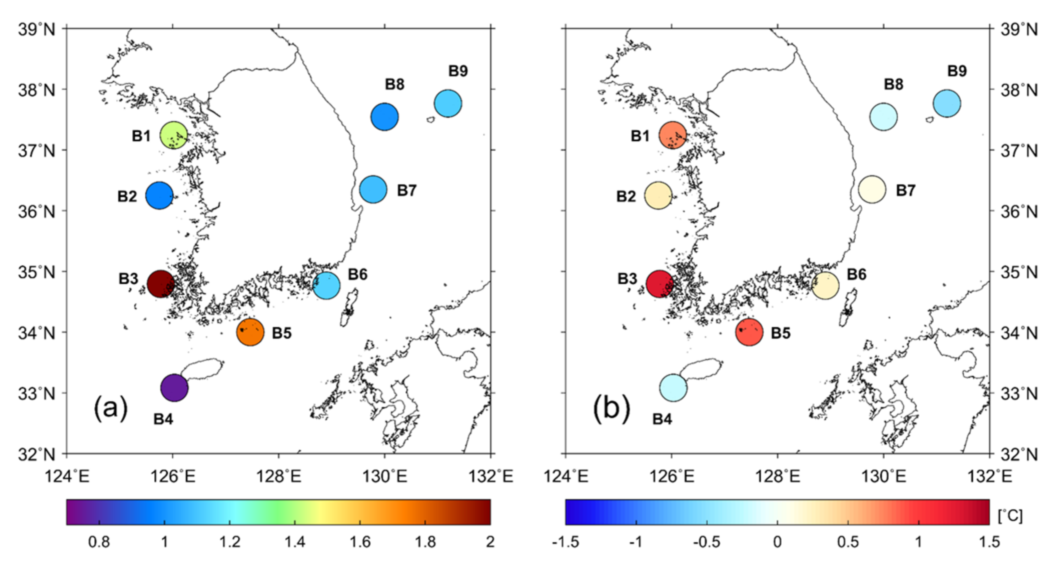
In Korean coastal regions, many coastal buoys, including wave buoys, have measured the water temperature for many decades [25]. Excluding the wave buoys located close to the coastlines (0.14–13.36 km), operated for a short period since 2014 [25], the temperature measurements at the nine stations (B1 to B9) were compared with daily OISST to assess SST accuracy in coastal regions, as shown in Figure 1b. As a result, most OISSTs produced RMSEs ranging from 0.75 K (B4, Marado) to 1.99 K (B3, Chilbaldo) and bias from −0.51 K (B9, Ulleungdo) to 1.27 K (B3, Chilbaldo) (Figure 2). Except for the two buoys (B2 and B4) with relatively small RMSEs of approximately 0.97 K and 0.75 K, most buoys exhibited large differences exceeding 1.00 K such as B1 (1.42 K), B3 (1.99 K), B5 (1.76 K), B6 (1.13 K), B7 (1.08 K), B8 (1.00 K), and B9 (1.11 K) (Figure 3a). The bias ranged from −0.21 K (B4) to 1.27 K (B3) (Figure 3b).
Although most stations are a few tens of kilometers away from land, the RMSE and bias were larger than the previously reported values in the open ocean. Overall, the RMSE tends to be relatively large at coastal buoys in the YS and southern regions than in the EJS. Large temperature differences of this type, amounting to 2 K, have been mentioned as induced by strong tidal currents and mixing over shallow bathymetry (<30 m) in the YS [25,57,58]. The western and southern coastal regions contained a positive bias of the differences (B1, B2, B3, B5, and B6), which are in contrast to the negative biases at the buoys (B8 and B9) over deep water (>1500 m) in the EJS.
In particular, the southwestern coastal region near the station B3 is known to have the strongest tidal currents, amounting to 1.2–5.8 m s−1 at the maximum, especially at Uldolmok (34.57°N, 126.30°E), when compared with other stations (http://www.khoa.go.kr; [59]). Such strong tidal currents cause vigorous vertical mixing over shallow bathymetry in the summer, inducing cold seawater to rise from the lower to the upper layers of sea water [60]. As a result, sea fog occurs frequently in the summer due to air–sea interaction, making it difficult to calculate SST from AVHRR data. Therefore, the environment of the coast of the YS has caused such large RMSEs of OISSTs at the station B3 (Chilbaldo) in the southwestern coastal region.
4.2. Comparison of SSTs and KODC Temperature Measurements
Similar to the comparison at the KMA buoy points (Figure 3), the OISST data were collocated with water temperatures measured at the KODC observation stations. The OISSTs in the seas around Korea produced relatively high RMSEs, from 1.22 K in the EJS to 1.37 K in the YS and the southern region (Figure 4). The overall accuracy of the OISSTs showed an RMSE of 1.31 K and a bias of 0.31 K for 37 years (1982 to 2018). Nevertheless, the histogram of the number density in Figure 4 shows the maximum values with high frequency on the linear line between the satellite and in situ temperatures.
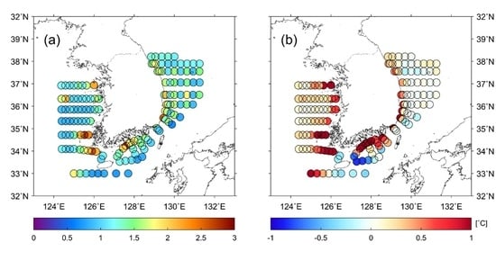
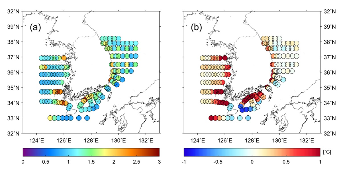
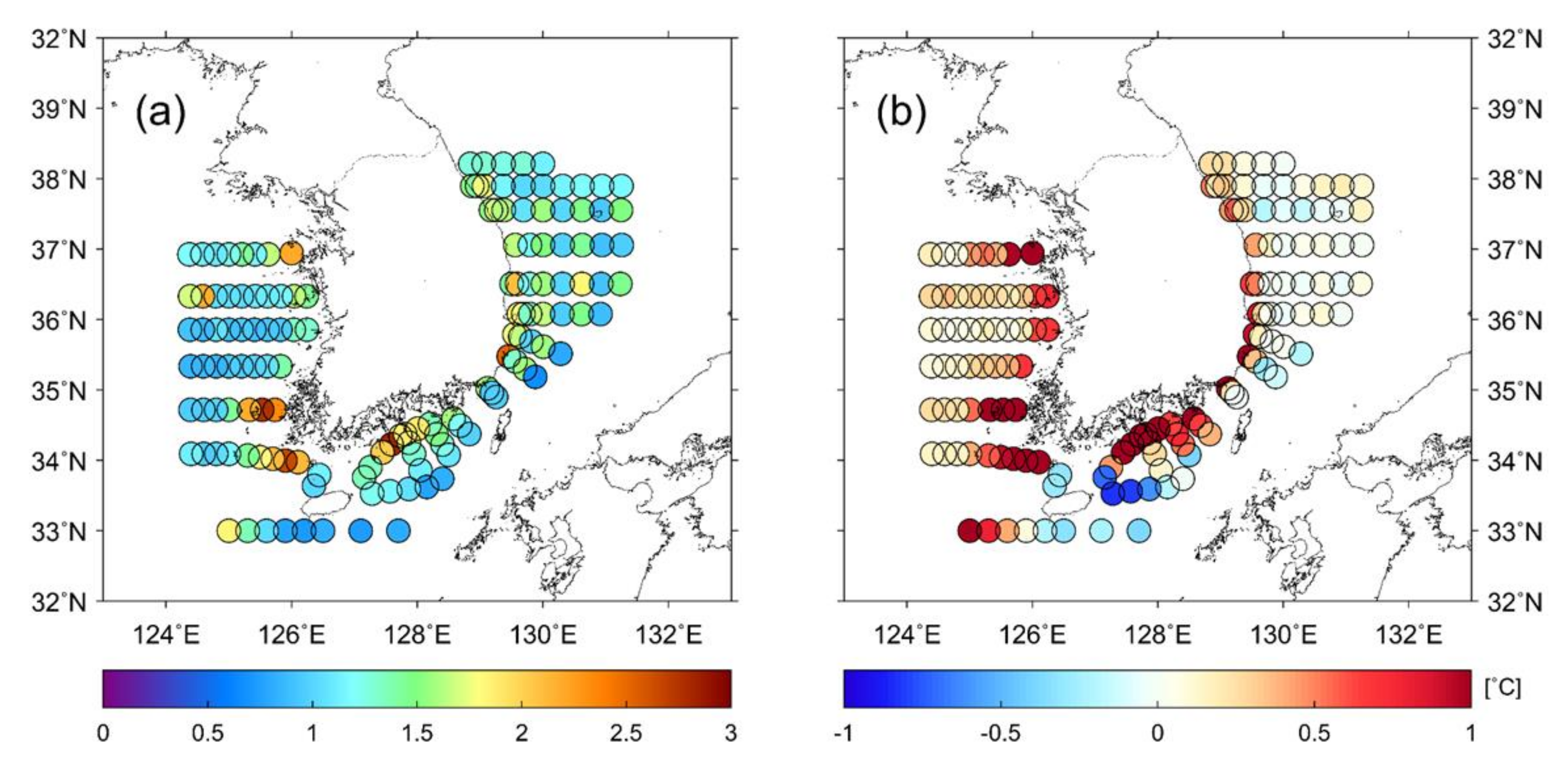
Figure 5 shows the spatial distribution of the RMSE and bias at the KODC stations. Most RMSE values ranged from 0.50 K to 1.50 K; however, high differences amounting to or exceeding 2.50 K were found near the coastal regions, especially near the southwestern corners of the Korean Peninsula, as shown in the station B3 (Chilbaldo) in the YS. This high RMSE was also observed near the station B5 in the southern coastal region. One of the peculiar trends in the spatial distribution is that the RMSEs tend to increase from 0.50 K to 1.50 K when approaching the coastline from far-offshore regions with an RMSE of less than 0.50 K (Figure 5a). Since the water depth is very deep in the EJS, the coastal areas of the EJS were inferred to have relatively small differences. However, the eastern coasts also yielded higher RMSE values similar to those of the western and southern coastal regions. The spatial distribution of the bias, as shown in Figure 5b, was similar to that of the RMSEs exhibiting noticeable differences in the coastal region. In the offshore area in the EJS, the satellite SST biases are weakly negative at approximately −0.3 K, implying that satellite OISSTs tend to be weakly underestimated as compared to the in situ temperatures (Figure 5b).
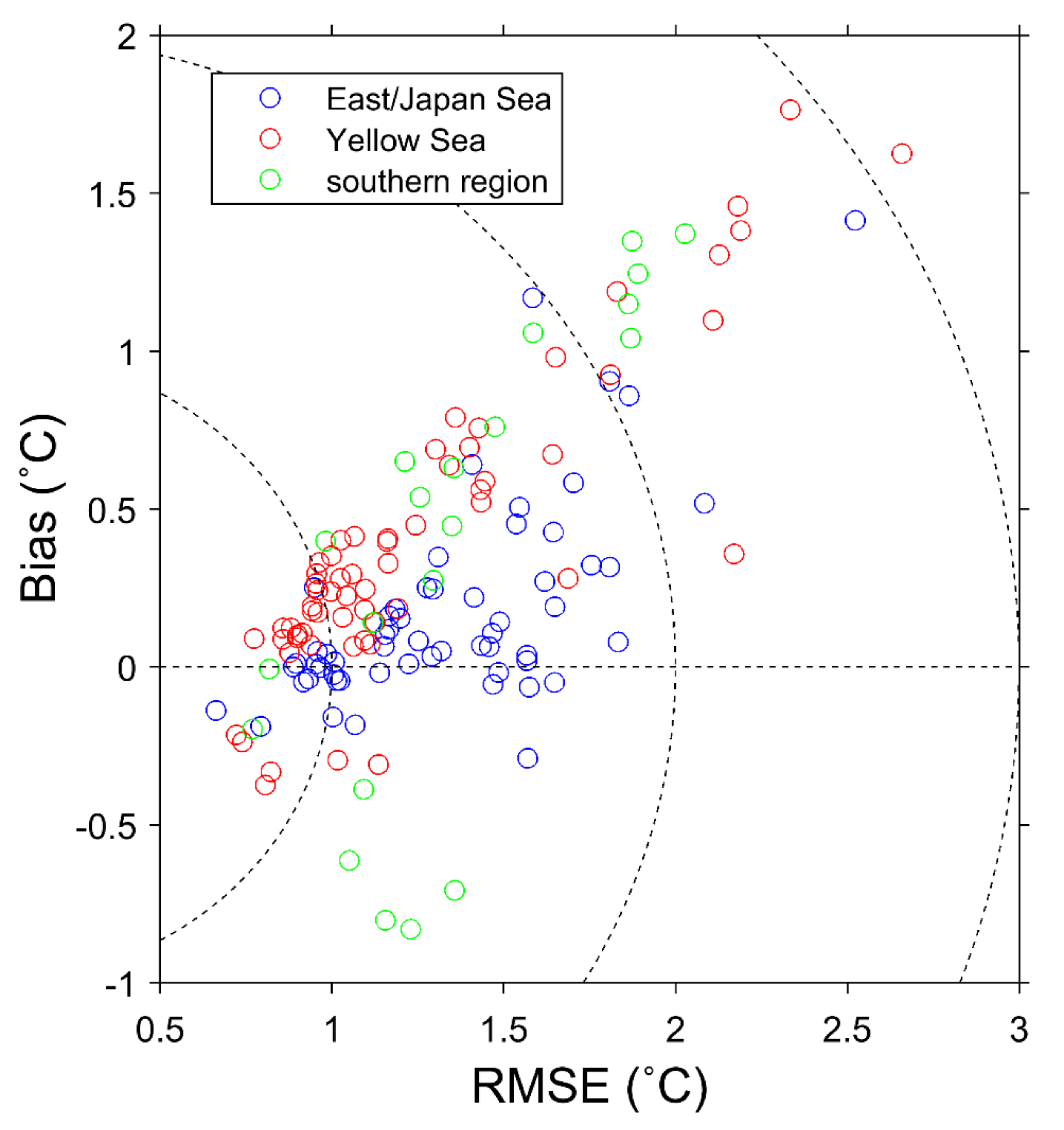
Figure 6 shows a scatter plot of the RMSE and bias in the EJS (north of Tsushima Island), YS (west of Jeju Island), and southern region (between Jeju Island and Tsushima Island). As described earlier, the differences in the EJS, as marked in blue circles, are relatively small compared with those of the YS (red circles) and the southern region (green circles). Most dots were distributed in the positive bias error region, implying a general tendency of higher satellite SSTs than in situ temperatures.
4.3. Elevated SST Differences at Near-Coastal Regions
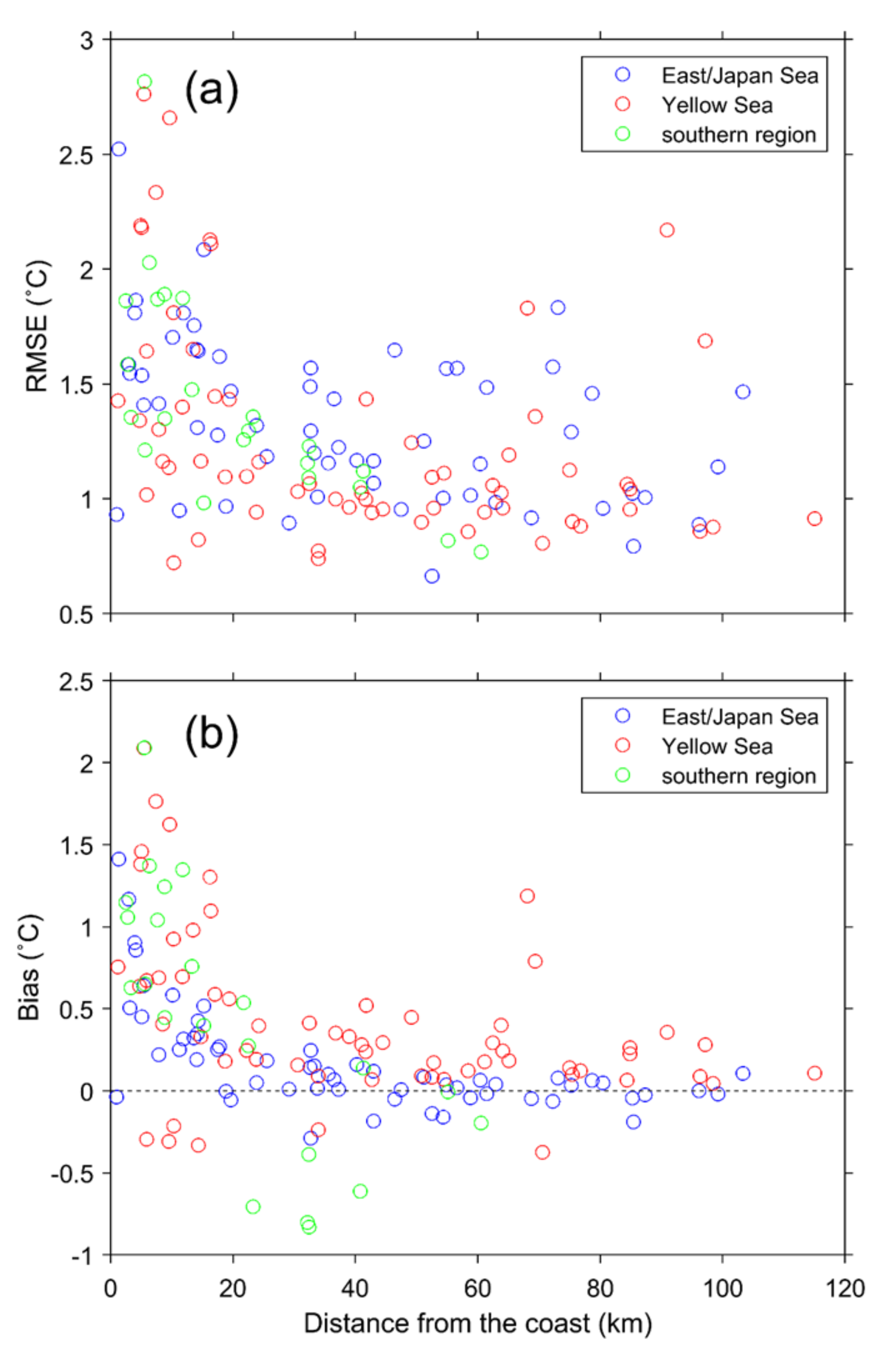
The previous analysis revealed a tendency for OISST differences to be augmented in near-coastal regions. To determine to what extent the tendency is augmented, the dependence of SST differences on the distance from the coastline was investigated. Figure 7a indicates that the highest RMSE is 2.80 K 5 km from the coastline. The RMSEs show a sharp decline to approximately 1.5 K at about 20–30 km, and then tend to increase to about 100 km in the offshore region. Regardless of the local characteristics, the three regions showed exponentially decaying relations of the SST RMSE at less than 25 km from the coast (Figure 7a).
The bias values of the three regions also show the dependence on the distance from the coast, as shown in Figure 7b. Within 40 km of the coast, the OISSTs have large scatters of bias of less than approximately 2.1 K. In contrast, these biases are considerably reduced within 0.5 K at longer distances from 20 km to 120 km. The coastal region of the YS has high positive bias at all distances from the coastline. This indicates that the greater the distance from the coast, the smaller the bias error.
4.4. Long-Term Trend of Satellite SST
As shown earlier, the satellite SSTs had different accuracies in the offshore seas and near-coast regions of the Korean Peninsula. Most of our understanding about the recent rapid warming of the ocean has depended on the results of an analysis using satellite databases since 1980. In order to understand the oceanic response and its role in climate change, the long-term trends need to be verified as similar to the satellite SSTs. Therefore, the SST trend was calculated using 37-year OISST data from 1982 to 2018 and we tested whether it was statistically significant within a confidence level of 95% using the Mann‒Kendall test.
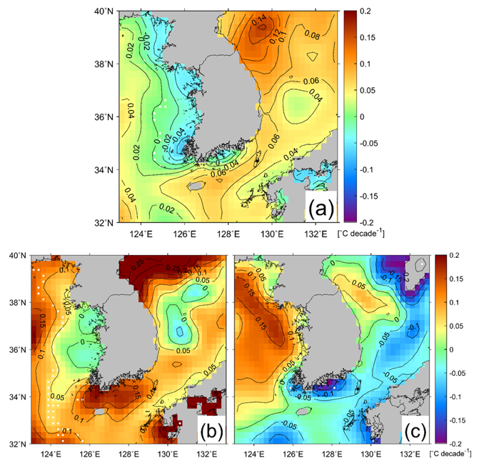
The estimated SST trends ranged from −0.07 °C decade−1 to 0.16 °C decade−1, with statistical significance (Figure 8a). The western and eastern seas of the Korean Peninsula are different from each other in various ways such as water depth differences and warm or cold currents (Figure 1a), such that the long-term change in SSTs revealed dissimilarity with respect to local characteristics. All the eastern seas of the EJS have positive trends at approximately 0.16 °C decade−1, with the highest trends (>0.12 °C decade−1) in the northern part of the EJS and a weak warming of approximately 0.04 °C decade−1 in the southern part of the EJS. In contrast to such warming trends, the coastal region off the western coasts revealed weakly negative values of approximately −0.03 °C decade−1. This cooling feature is limited to the coastal area, approximately 100 km from the coastline. There are only a few pixels with statistically insignificant trends within the 95% confidence level, as indicated by the white dots in Figure 8. The coastal region of the YS has experienced continuous warming since the 1980s, according to a previous report of the warming rate for the period from 1981 to 2009 [61], which is the opposite of the cooling trend in Figure 8a. This seems to be associated with the frequent appearance of very low water temperatures in the coastal area induced by severe cold-air outbreaks in winter due to the recent warming of the Arctic Ocean and the weakening of the westerlies in the mid-latitude regions since 2000 [54,62,63].
Figure 8b,c shows the OISST trends for each 19-year period (1982 to 2000 and 2000 to 2018), which demonstrates the opposite trend along the coastal region of the YS. This is reported to be related to the effect of global warming hiatus on the reduction in coastal SST warming. Because the water depth of the coastal area of the YS is very shallow (less than 30 m), the atmospheric environment can possibly modify the local response of SSTs in coastal areas. This recent cooling-off along the western coast has been reflected in the total trend over the entire period, resulting in weak cooling along the west coast.
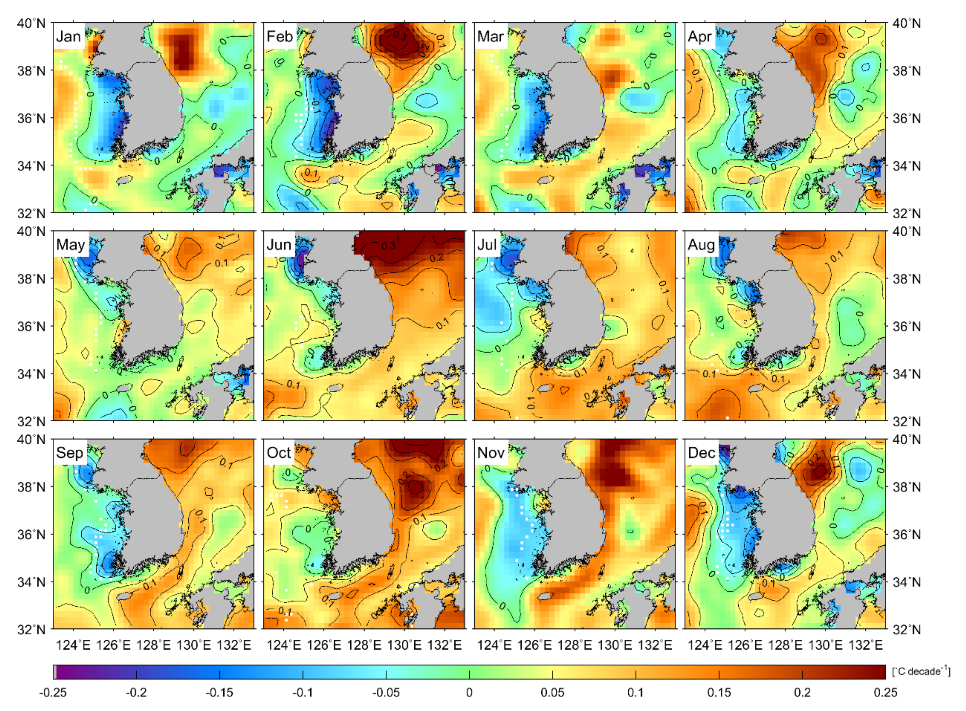
Figure 9 shows the monthly variations of the long-term SST trend for the entire period from 1982 to 2018. The trends are overall similar to the total trend in Figure 8a for every month except June. In the EJS, the positive SST trend appeared broadly up to 0.34 °C decade−1 in the entire EJS. In the YS, monthly trends were positive in the offshore region and negative in the near-coastal region. However, the seasonal trend of the near-coastal region showed relatively high warming rates of about 0.08 °C decade−1, centered at 125.6°E, 36.4°N in August. This implies that the weakly negative SST cooling along the near-coastal region in the YS in Figure 8a was led not by the trend in summer but by that in winter, especially in February (Figure 9).
4.5. Long-Term Trend of In Situ Temperatures
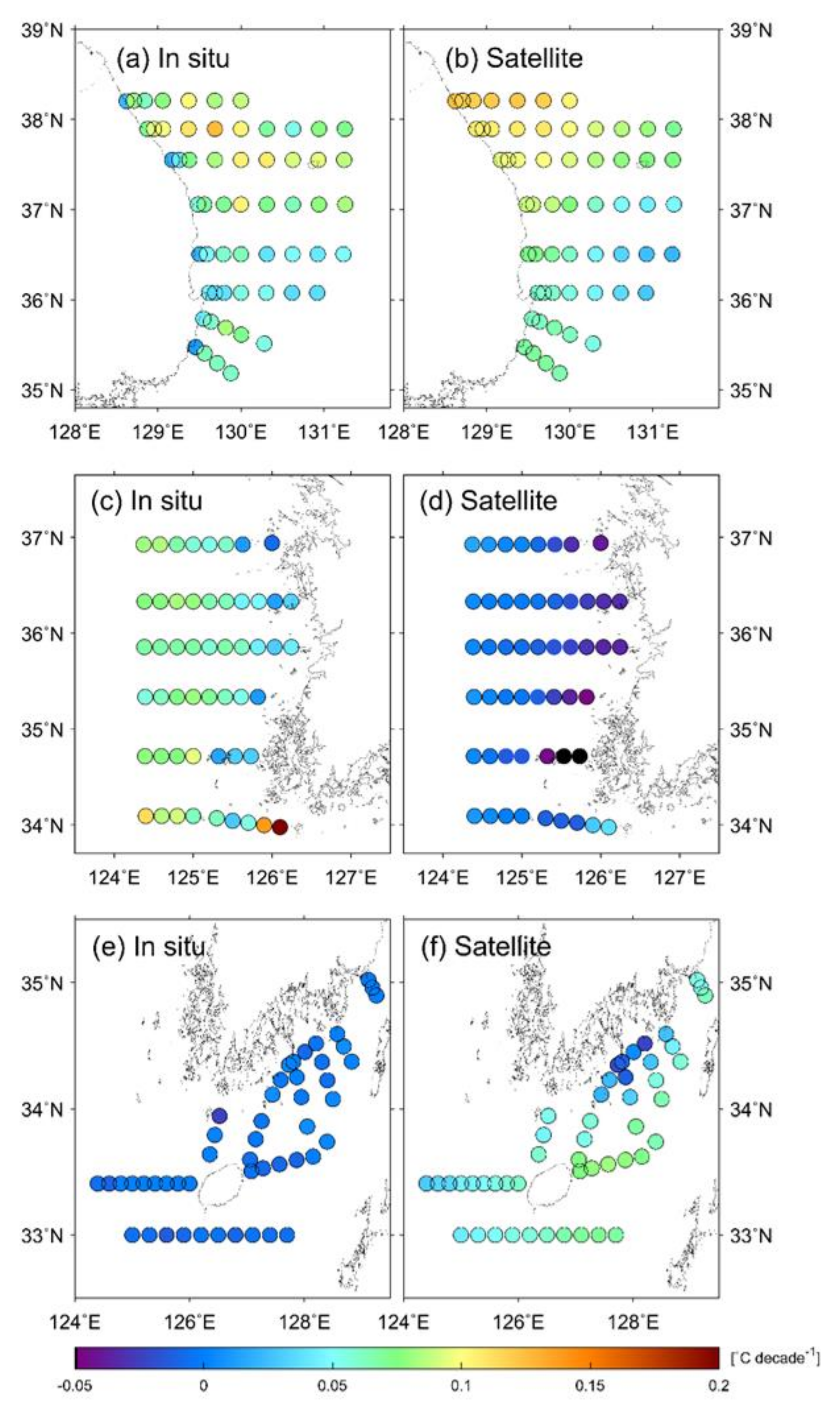
Figure 10 shows the spatial distribution of the temporal trends of the KODC in situ surface temperatures in the eastern, western, and southern coastal regions of the Korean Peninsula. All trends of the KODC stations in the EJS exhibited positive values, corresponding to weak warming (<0.05 °C decade−1) along the coasts, and relatively high warming trends, amounting to 0.13 °C decade−1 in the offshore stations (Figure 10a). In particular, the trends of SSTs in the northern stations over 37°N presented more prominent warming than those of the southern stations (<36°N). Comparing this warming tendency with the trends of satellite SSTs in Figure 10b, both the satellite and in situ SST trends are similarly distributed in the range of 0.02–0.15 °C decade−1. Another similar feature is that the trends are slightly low at the stations near/along the coastlines, and relatively high in the offshore and the northern regions. This suggests the potential capability of satellite OISSTs to represent actual SST changes regardless of the differences and accuracies of satellite SSTs.
It is still unclear whether the satellite SSTs of the YS, with relatively high RMSE and bias, can represent the rate of change in the long-term actual surface temperatures despite the shallow water depth and strong tidal currents in the YS. To investigate this issue, satellite SST trends in the YS were also compared with the KODC trends of the surface temperatures for the entire period (Figure 10c,d). Figure 10c shows a characteristic pattern of KODC SST warming rates (<0.20 °C decade−1) with relatively little warming on the coastal side and relatively high warming in the offshore regions of the YS. There are gradually increasing tendencies of the warming rates along the given lines of the KODC stations. Similar to this tendency of the in situ temperature trends, the OISST trends also revealed a similar spatial pattern, with increasing trends from the near coast to the offshore region. However, the magnitudes of the OISST trends are remarkably different, revealing negative trends, i.e., SST cooling, near the coastal regions. All the trends at the KODC stations are statistically significant within 95% over the period 1982–2018.
Similar to the western coast, the southern coastal region is well known for its shallow bathymetry, many islands, strong tidal currents, and thermal fronts. Figure 10e,f shows the long-term trends of the OISSTs and KODC in situ temperatures, respectively. Unlike the EJS and YS, there are considerable differences in the temporal trends between satellite SSTs and in situ temperatures without any consistent spatial structure of increasing or decreasing trends.
4.6. Comparison of SST Trends from Satellite and In Situ Data
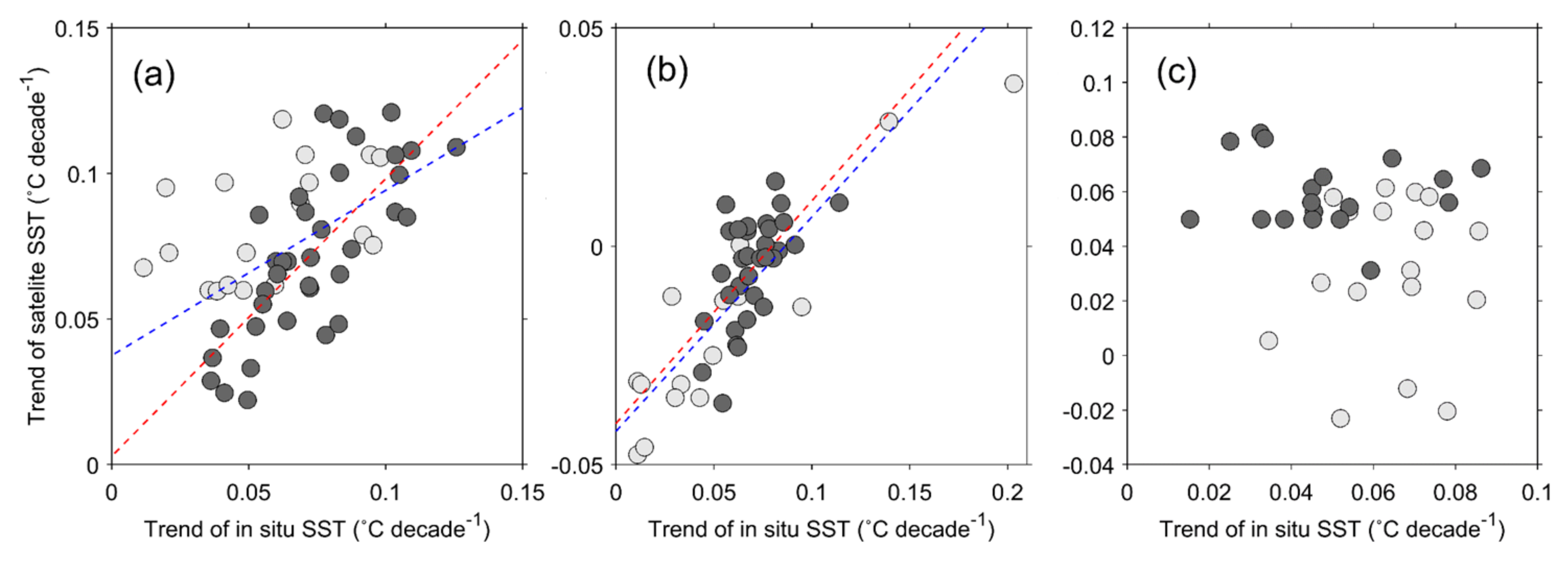
We examined the quantitative consistency of the satellite SST trends at the coastal stations with the trends calculated from actually observed water temperatures in Figure 10. In the case of the EJS (Figure 11a), the overall trend values of the satellite SSTs showed a positive relation to those of in situ temperatures. However, the least-squared fitted line in blue has a low statistical significance for R2 (0.30). When the trends of the KODC stations within 0.25° of the shoreline were excluded, the accuracy of the long-term trends at the offshore stations improved with a linear relation of approximately 0.95 (R2 = 0.57), as indicated by the red dashed fitted line to the dark gray dots (Figure 11a).
The spatial distribution of the satellite SST trends in the YS was quite similar to the trends of in situ temperature variations in spite of the overall shift of the magnitudes, as denoted in Figure 10b. Another characteristic difference was the reverse trend, demonstrating negative trends of satellite SSTs, contrasting the positive trends of in situ temperatures near/along the coastal area. Despite the differences in absolute values, such a spatial similarity expressed a linear relationship of 0.49 (R2 = 0.65) for all of the stations, as shown by the least-squared fitted blue line in Figure 11b. These trends were biased but highly correlated with smaller scatters than the EJS. Exclusion of the near-coastal stations presented a linear slope of 0.51 (R2 = 0.35) with slight improvement, as indicated by the red dashed line.
Unlike the cases of the EJS and YS, the southern coastal regions did not yield any consistent relationship between the trends from satellite SSTs and in situ SSTs (Figure 11c). The in situ trends in Figure 11c are mostly concentrated around the values from 0.01 °C decade−1 to 0.09 °C decade−1. In contrast, the satellite SST trends contained slight cooling trends reaching approximately −0.02 °C decade−1 at the near-coast stations (around 34.3°N, 127.5°E), as denoted in Figure 10f. Removal of near-coastal data (<0.25° from the coastline) did not provide a consistent relationship in this southern coastal region. Local oceanic conditions, such as complex coastal lines, island wakes, topography, fronts, tidal currents, or other atmospheric and oceanic environments, might contribute to such inconsistencies in satellite-based SST trends.
5. Discussion
5.1. Potential Causes of Coastal Satellite SST Differences
Both the buoy temperatures and in situ temperatures demonstrated higher RMSE and positive bias differences of OISSTs at near-coast regions than in the offshore regions. Such a tendency was detected in the entire near-coast region along the coastline of the Korean Peninsula, including the YS and the EJS. With regard to the highest RMSE and warm bias in the YS, previous studies have addressed the role of dominant mixing induced by strong tidal currents over shallow bathymetry in case of such differences [25,57,58]. Because of sea fog and frequent cloudy conditions over upwelled cold waters, the AVHRR-based OISST under clear sky conditions probably have few pixels at the stations. The absence of these types of SSTs is likely to facilitate neighboring SST values with relatively high temperatures in the far-offshore regions to be given in producing SST composites in the procedure of optimal interpolation (OI). Through the OI procedure, the tendency of warm bias and high RMSEs would be dispersed in the near-coast regions. Although microwave SST observations of other global SST products can overcome the cloudy conditions, they are also expected not to play an important role in the SST OI procedure, partly because of the interference of microwave observations near landmass areas along the coastlines [25]. Thus, the differences of these types at the near-coast regions can be reduced by incorporating as many in situ temperatures as possible into the OI procedure as input data.
More importantly, the discrepancies herein may also be related to different sampling characteristics in time and space. The OISST and in situ SST are fundamentally different because satellite SST is an averaged temperature of all radiations over a pixel, while in situ temperature is obtained at a specific point. It was reported that spatial separations of about 10 km and time intervals of about 2 h could produce an RMSE of about 0.2 K in the validation of satellite SSTs [64]. The two temperatures are not the same SST but substantially different at the near-coastal regions because of high spatial scale differences and the temporal variability of submesoscale oceanic features.
Moreover, it should be noted that strong SST gradients in the coastal zone are not resolved in lower-resolution OISST images [26]. In the southern near-coastal regions, many island-induced wake variabilities can also yield warm or cold bias in the satellite SSTs relative to the in situ measurements. All of these variability on scales smaller than the spatial resolution of the OISST dataset may introduce the discrepancies. Relatively high RMSE and bias values can be also induced by skin-bulk differences originating from the different water depths of temperature measurements, i.e., 2–3 m at the KODC stations, about 20 cm at the KMA buoy station, and near the sea surface of OISST. Complicated small-scale oceanic features of these types can contribute to the temperature differences in the coastal regions than in the open ocean.
5.2. Potential of Satellite SST Trends
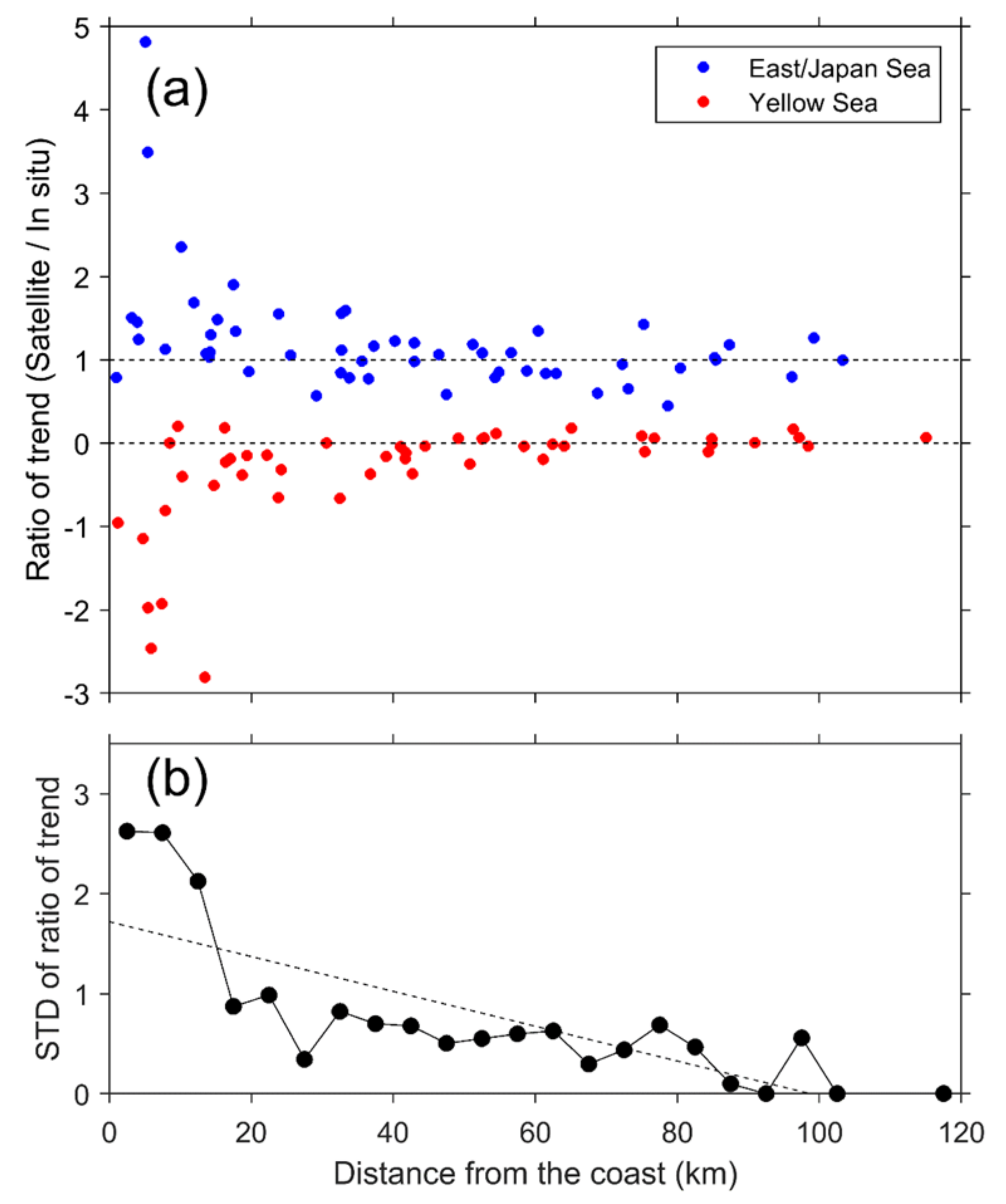
The long-term trends of satellite SST variations along the Korean coast tended to increase as the in situ temperatures increased, regardless of the overestimation tendency and warm bias of SSTs at near-coast regions. Overall, the results of this study suggest that the satellite-observed SST trends could be stably used in offshore areas where water depth is relatively deeper and tidal currents are much weaker than the near-coast regions. Satellite-based SST trends explain 99% of the trends of in situ temperatures in the offshore region, except for the alongshore region (<25 km) in the EJS, as shown in the blue dots of Figure 12a. In contrast to the EJS, the credibility of this SST trend in the offshore region of the YS was considerably reduced to the KODC temperature trends at the same range of distances (>25 km) as indicated by red dots (Figure 12a). As for the coastline (<25 km), the ratios of the near-coast SST trends increase rapidly by 1.89 in the EJS and decrease down to −0.75 in the YS. This implies that the accuracy of SST trends based on satellite observations is likely to be significantly reduced in the near-coast regions compared to the offshore regions. Overall, the standard deviation (STD) of the ratios of the SST trends for both the EJS and the YS, as indicated in Figure 12b, is inversely correlated to the distance from the coast (x), with a linear relationship (STD = −0.01x + 1.70).
The dominant factors in such different ratios are attributed to diverse changes in local air–sea conditions from complicated bathymetry, tidal currents and mixing, turbidity, sea fog, and clouds. Another factor influencing near-shore satellite-derived SSTs could be submesoscale SST variability, as observed in the Landsat SST images [26]. The findings of this study could be helpful for understanding the warming or cooling rates in coastal regions with various characteristics of local seas. In contrast to the global ocean, the coastal regions of marginal seas are likely to have different credibility of the estimated SST trends depending on the local marine and atmospheric environments of in situ observation stations in coastal regions. In addition to the local SST differences, more detailed studies on the long-term trends of SSTs in the local seas are needed for diverse applications of the coastal regions using satellite-based SST products of the global ocean. Instrument degradation of AVHRR should also be further studied in the local seas, as emphasized in [20].
6. Conclusions
Satellite-observed SSTs have long been used to understand short-term SST variations as well as long-term temperature trends over decades. Considering the diverse applications of satellite SSTs in regions within a few hundreds of kilometers of the coastline, the accuracy assessment of OISSTs is essential because the OISST database is one of the most representative SST products and has the longest temporal period, from September 1981 onwards. In addition, it is important to understand the characteristics of the long-term SST trends from satellite data in the global ocean as well as coastal regions. Through the validation of the SSTs and the long-term trends with respect to in situ temperature measurements over decades, this study examined the reliability of satellite SSTs with respect to real temperature variations.
This study assessed the accuracy of the OISST data by comparing them with in situ measurements from the KMA buoys and the KODC stations in coastal regions around the Korean Peninsula from 1982 to 2018. The accuracy of OISSTs revealed some dependence on water depth as well as the distance from the coastline. In addition, SST differences tended to be amplified with proximity to near-coastal regions. Atmospheric conditions are believed to affect the infrequent observations of SST, especially in the southwestern coastal region of the Korean Peninsula. Such a lack of coastal SST observations produced a positive bias and relatively higher RMSE in near-coastal regions than in far-offshore regions. Other factors, such as skin-bulk differences, diurnal variations, spatial-scale differences of coastal oceanic phenomena including submesoscale SST variability, and the stability condition of the marine‒atmospheric boundary layer, can contribute to differences between the OISSTs and in situ temperatures, as summarized in [65]. In addition, differences between satellite sensors, as well as the drifts in a single sensor that occur over a satellite’s lifetime, may contribute to discrepancies in temperature [20].
Nevertheless, the overall long-term trend of satellite SSTs agreed with 99% of that of in situ temperatures in the offshore region of the EJS (>25 km) over several decades, with a consistent direction of warming, depending on the locations of the buoys and the stations in the coastal regions. This suggests the use of long-term satellite OISSTs in the understanding of changes in the coastal temperature. Although this study focused on OISST variations in limited Korean coastal regions, it can be extended to other coastal regions across the global ocean. Additionally, it would be worthwhile to conduct similar studies on other global SST datasets. The present results demonstrated the characteristic features of SST trends in Korean coastal regions with increasing vulnerability to climate change. Thus, further studies should be performed to understand how the present satellite SST analyses represent actual temperature trends in the near-coast and offshore coastal regions under rapidly changing climate conditions.
Author Contributions
Conceptualization, K.-A.P.; data curation, E.-Y.L.; methodology, K.-A.P. and E.-Y.L.; writing—original draft preparation, E.-Y.L.; writing—review and editing; K.-A.P. and E.-Y.L. All authors have read and agreed to the published version of the manuscript.
Funding
This research was funded by the National Research Foundation of Korea (NRF), via a grant funded by the Korean government (MSIT) (No. 2020R1A2C2009464).
Acknowledgments
NOAA OISST V2 data were provided by the NOAA/OAR/ESRL PSD, Boulder, CO, USA, https://www.esrl.noaa.gov/psd. The authors also thank KMA and KODC for providing in situ water temperature data.
Conflicts of Interest
The authors declare no conflict of interest.
References
- Good, P.; Lowe, J.A.; Rowell, D.P. Understanding uncertainty in future projections for the tropical Atlantic: Relationships with the unforced climate. Clim. Dyn. 2009, 32, 205–218. [Google Scholar] [CrossRef]
- Ashfaq, M.; Skinner, C.B.; Diffenbaugh, N.S. Influence of SST biases on future climate change projections. Clim. Dyn. 2011, 36, 1303–1319. [Google Scholar] [CrossRef]
- Strong, A.E.; McClain, E.P. Improved ocean surface temperatures from space—Comparisons with drifting buoys. Bull. Am. Meteorol. Soc. 1984, 65, 138–142. [Google Scholar] [CrossRef] [Green Version]
- McClain, E.P. Global sea surface temperatures and cloud clearing for aerosol optical depth estimates. Int. J. Remote Sens. 1989, 10, 763–769. [Google Scholar] [CrossRef]
- Barton, I. Satellite-derived sea surface temperature: Current status. J. Geophys. Res. 1995, 100, 8777–8790. [Google Scholar] [CrossRef]
- Walton, C.C.; Pichel, W.G.; Sapper, J.F.; May, D.A. The development and operational application of nonlinear algorithms for the measurement of sea surface temperatures with the NOAA polar-orbiting environmental satellites. J. Geophys. Res. Oceans 1998, 103, 27999–28012. [Google Scholar] [CrossRef]
- Tanahashi, S.; Kawamura, H.; Matsuura, T.; Takahashi, T.; Yusa, H. Improved estimates of wide-ranging sea surface temperature from GMS S-VISSR data. J. Oceanogr. 2000, 56, 345–358. [Google Scholar] [CrossRef]
- Kilpatrick, K.A.; Podesta, G.P.; Evans, R. Overview of the NOAA/NASA Advanced Very High Resolution Radiometer Pathfinder algorithm for sea surface temperature and associated matchup database. J. Geophys. Res. 2001, 106, 9179–9198. [Google Scholar] [CrossRef]
- Brisson, A.; Borgne, P.L.; Marsouin, A. Results of one year preoperational production of sea surface temperatures from GOES-8. J. Atmos. Ocean. Technol. 2000, 19, 1638–1652. [Google Scholar] [CrossRef]
- Guan, L.; Kawamura, H. Merging satellite infrared and microwave SSTs: Methodology and evaluation of the new SST. J. Oceanogr. 2004, 60, 905–912. [Google Scholar] [CrossRef]
- Dong, S.; Gille, S.T.; Sprintall, J.; Gentemann, C. Validation of the Advanced Microwave Scanning Radiometer for the Earth Observing System (AMSR-E) sea surface temperature in the Southern Ocean. J. Geophys. Res. 2006, 111, C04002. [Google Scholar] [CrossRef]
- O’Carroll, A.G.; Watts, J.G.; Horrocks, L.A.; Saunders, R.W.; Rayner, N.A. Validation of the AATSR Meteo product sea surface temperature. J. Atmos. Ocean. Technol. 2006, 23, 711–726. [Google Scholar] [CrossRef] [Green Version]
- Haines, S.L.; Jedlovec, G.J.; Lazarus, S.M. A MODIS sea surface temperature composite for regional applications. IEEE Trans. Geosci. Remote Sens. 2007, 45, 2919–2927. [Google Scholar] [CrossRef]
- Lazarus, S.M.; Calvert, C.G.; Splitt, M.E.; Santos, P.; Sharp, D.W.; Blottman, P.F.; Spratt, S.M. Real-time, high-resolution, space–time analysis of sea surface temperatures from multiple platforms. Mon. Weather Rev. 2007, 135, 3158–3173. [Google Scholar] [CrossRef] [Green Version]
- Merchant, C.J.; Le Borgne, P.; Marsouin, A.; Roquet, H. Optimal estimation of sea surface temperature from split-window observations. Remote Sens. Environ. 2008, 112, 2469–2484. [Google Scholar] [CrossRef]
- Gentemann, C.L.; Meissner, T.; Wentz, F.J. Accuracy of satellite sea surface temperatures at 7 and 11 GHz. IEEE Trans. Geosci. Remote Sens. 2009, 48, 1009–1018. [Google Scholar] [CrossRef]
- Vázquez-Cuervo, J.; Armstrong, E.M.; Casey, K.S.; Evans, R.; Kilpatrick, K. Comparison between the Pathfinder versions 5.0 and 4.1 sea surface temperature datasets: A case study for high resolution. J. Clim. 2010, 23, 1047–1059. [Google Scholar] [CrossRef]
- Beggs, H.; Zhong, A.; Warren, G.; Alves, O.; Brassington, G.; Pugh, T. RAMSSA—An operational, high-resolution, regional Australian multi-sensor sea surface temperature analysis over the Australian region. Aust. Meteorol. Oceanogr. J. 2011, 61, 1. [Google Scholar] [CrossRef]
- Kurihara, Y.; Murakami, H.; Kachi, M. Sea surface temperature from the new Japanese geostationary meteorological Himawari-8 satellite. Geophys. Res. Lett. 2016, 43, 1234–1240. [Google Scholar] [CrossRef] [Green Version]
- Merchant, C.J.; Embury, O.; Bulgin, C.E.; Block, T.; Corlett, G.K.; Fiedler, E.; Good, S.A.; Mittaz, J.; Rayner, N.A.; Berry, D.; et al. Satellite-based time-series of sea-surface temperature since 1981 for climate applications. Sci. Data 2019, 6, 223. [Google Scholar] [CrossRef] [PubMed] [Green Version]
- Li, X.; Pichel, W.; Clemente-Colon, P.; Krasnopolsky, V.; Sapper, J. Validation of coastal sea and lake surface temperature measurements derived from NOAA/AVHRR data. Int. J. Remote Sens. 2001, 22, 1285–1303. [Google Scholar] [CrossRef]
- Smit, A.J.; Roberts, M.; Anderson, R.J.; Dufois, F.; Dudley, S.F.; Bornman, T.G.; Olbers, J.; Bolton, J.J. A coastal seawater temperature dataset for biogeographical studies: Large biases between in situ and remotely-sensed data sets around the coast of South Africa. PLoS ONE 2013, 8, e81944. [Google Scholar] [CrossRef] [PubMed] [Green Version]
- Calson, D.F.; Yarbro, L.A.; Scolaro, S.; Poniatowski, M.; McGee-Absten, V.; Carlson, P.R., Jr. Sea surface temperatures and seagrass mortality in Florida Bay: Spatial and temporal patterns discerned from MODIS and AVHRR data. Remote Sens. Environ. 2018, 208, 171–188. [Google Scholar] [CrossRef]
- Brewin, R.J.W.; de Mora, L.; Billson, O.; Jackson, T.; Russell, P.; Brewin, T.G.; Shutler, J.; Miller, P.I.; Taylor, B.H.; Smyth, T.J.; et al. Evaluating operational AVHRR sea surface temperature data at the coastline using surfers. Estuar. Coast. Shelf Sci. 2017, 196, 276–289. [Google Scholar] [CrossRef]
- Woo, H.-J.; Park, K.-A. Inter-comparisons of daily sea surface temperatures and in-situ temperatures in the coastal regions. Remote Sens. 2020, 12, 1592. [Google Scholar] [CrossRef]
- Jang, J.-C.; Park, K.-A. High-resolution sea surface temperature retrieval from Landsat 8 OLI/TIRS data at coastal regions. Remote Sens. 2019, 11, 2687. [Google Scholar] [CrossRef] [Green Version]
- Kim, H.-Y.; Park, K.-A. Comparison of Sea Surface Temperature from Oceanic Buoys and Satellite Microwave Measurements in the Western Coastal Region of Korean Peninsula. J. Korean Earth Sci. Soc. 2018, 39, 555–567. [Google Scholar] [CrossRef]
- IPCC. Climate Change 2014: Synthesis Report. Contribution of Working Group I, II and III to the Fifth Assessment Report of the Intergovernmental Panel on Climate Change; Core Writing Team, Pachauri, R.K., Meyer, L.A., Eds.; IPCC: Geneva, Switzerland, 2014; p. 151. [Google Scholar]
- Easterling, D.R.; Wehner, M.F. Is the climate warming or cooling? Geophys. Res. Lett. 2009, 36, L08706. [Google Scholar] [CrossRef] [Green Version]
- Kaufmann, R.K.; Kauppi, H.; Mann, M.L.; Stock, J.H. Reconciling anthropogenic climate change with observed temperature 1998–2008. Proc. Natl. Acad. Sci. USA 2011, 108, 11790–11793. [Google Scholar] [CrossRef] [Green Version]
- Kosaka, Y.; Xie, S.P. Recent global-warming hiatus tied to equatorial Pacific surface cooling. Nature 2013, 501, 403. [Google Scholar] [CrossRef] [PubMed] [Green Version]
- Meehl, G.A.; Teng, H.; Arblaster, J.M. Climate model simulations of the observed early-2000s hiatus of global warming. Nat. Clim. Chang. 2014, 4, 898. [Google Scholar] [CrossRef] [Green Version]
- Steinman, B.A.; Mann, M.E.; Miller, S.K. Atlantic and Pacific multidecadal oscillations and Northern Hemisphere temperatures. Science 2015, 347, 988–991. [Google Scholar] [CrossRef] [PubMed] [Green Version]
- Karl, T.R.; Arguez, A.; Huang, B.; Lawrimore, J.H.; McMahon, J.R.; Menne, M.J.; Zhang, H.M. Possible artifacts of data biases in the recent global surface warming hiatus. Science 2015, 348, 1469–1472. [Google Scholar] [CrossRef] [PubMed] [Green Version]
- Hausfather, Z.; Cowtan, K.; Clarke, D.C.; Jacobs, P.; Richardson, M.; Rohde, R. Assessing recent warming using instrumentally homogeneous sea surface temperature records. Sci. Adv. 2017, 3, e1601207. [Google Scholar] [CrossRef] [PubMed] [Green Version]
- Belkin, I.M. Rapid warming of large marine ecosystems. Prog. Oceanogr. 2009, 81, 207–213. [Google Scholar] [CrossRef]
- Rayner, N.A.A.; Parker, D.E.; Horton, E.B.; Folland, C.K.; Alexander, L.V.; Rowell, D.P.; Kent, E.C.; Kaplan, A. Global analyses of sea surface temperature, sea ice, and night marine air temperature since the late nineteenth century. J. Geophys. Res. Atmos. 2003, 108, 4407. [Google Scholar] [CrossRef]
- Rayner, N.A.; Brohan, P.; Parker, D.E.; Folland, C.K.; Kennedy, J.J.; Vanicek, M.; Ansell, T.J.; Tett, S.F.B. Improved analyses of changes and uncertainties in sea surface temperature measured in situ since the mid-nineteenth century: The HadSST2 dataset. J. Clim. 2006, 19, 446–469. [Google Scholar] [CrossRef] [Green Version]
- Ohman, M.D.; Venrick, E.L. CalCOFI in a changing ocean. Oceanography 2003, 16, 76–85. [Google Scholar] [CrossRef] [Green Version]
- Hahn, S.D. SST warming of Korea coastal waters during 1881–1990. KODC Newsl. 1994, 24, 29–38. [Google Scholar]
- Kang, Y.Q. Warming trend of coastal waters of Korea during recent 60 years (1936–1995). Korean J. Fish. Aquat. Sci. 2000, 3, 173–179. [Google Scholar]
- Jeong, H.D.; Hwang, J.D.; Jung, K.K.; Heo, S.; Sung, K.T.; Go, W.J.; Yang, J.Y.; Kim, S.W. Long term trend of change in water temperature and salinity in coastal waters around Korean Peninsula. J. Korean Soc. Mar. Environ. Saf. 2003, 9, 53–57. [Google Scholar]
- Min, H.S.; Kim, C.H. Interannual variability and long-term trend of coastal sea surface temperature in Korea. Ocean Polar Res. 2006, 28, 415–423. [Google Scholar]
- Seong, K.-T.; Hwang, J.-D.; Han, I.-S.; Go, W.J.; Suh, Y.-S.; Lee, J.-Y. Characteristic for Long-term Trends of Temperature in the Korean Waters. J. Korean Soc. Mar. Environ. Saf. 2010, 16, 353–360. [Google Scholar]
- Kim, S.J.; Woo, S.H.; Kim, B.M.; Hur, S.D. Trends in sea surface temperature (SST) change near the Korean peninsula for the past 130 years. Ocean Polar Res. 2011, 33, 281–290. [Google Scholar] [CrossRef] [Green Version]
- Park, K.A.; Park, J.J.; Park, J.E.; Choi, B.J.; Lee, S.H.; Byun, D.S.; Lee, E.I.; Kang, B.S.; Shin, H.R.; Lee, S.R. Interdisciplinary Mathematics and Sciences in Schematic Ocean Current Maps in the Seas Around Korea. In Handbook of the Mathematics of the Arts and Sciences; Springer: Cham, Switzerland, 2019; p. 23. [Google Scholar]
- Reynolds, R.W.; Smith, T.M. A high-resolution global sea surface temperature climatology. J. Clim. 1995, 8, 1571–1583. [Google Scholar] [CrossRef]
- Reynolds, R.W.; Smith, T.M.; Liu, C.; Chelton, D.B.; Casey, K.S.; Schlax, M.G. Daily high-resolution-blended analyses for sea surface temperature. J. Clim. 2007, 20, 5473–5496. [Google Scholar] [CrossRef]
- Banzon, V.; Smith, T.M.; Chin, T.M.; Liu, C.; Hankins, W. A long-term record of blended satellite and in situ sea-surface temperature for climate monitoring, modeling and environmental studies. Earth Syst. Sci. Data 2016, 8, 165–176. [Google Scholar] [CrossRef] [Green Version]
- Banzon, V.; Smith, T.M.; Steele, M.; Huang, B.; Zhang, H. Improved Estimation of Proxy Sea Surface Temperature in the Arctic. J. Atmos. Ocean. Technol. 2020, 37, 341–349. [Google Scholar] [CrossRef]
- Good, S.A.; Corlett, G.K.; Remedios, J.J.; Noyes, E.J.; Llewellyn-Jones, D.T. The global trend in sea surface temperature from 20 years of advanced very high resolution radiometer data. J. Clim. 2007, 20, 1255–1264. [Google Scholar] [CrossRef] [Green Version]
- Weatherhead, E.C.; Reinsel, G.C.; Tiao, G.C.; Meng, X.-L.; Choi, D.; Cheang, W.-K.; Keller, T.; DeLuisi, J.; Wuebbles, D.J.; Kerr, J.B.; et al. Factors affecting the detection of trends: Statistical considerations and applications to environmental data. J. Geophys. Res. 1998, 103, 17149–17161. [Google Scholar] [CrossRef]
- Trenberth, K.E. Signal versus noise in the Southern Oscillation. Mon. Weather Rev. 1984, 112, 326–332. [Google Scholar] [CrossRef] [Green Version]
- Lee, E.-Y.; Park, K.-A. Change in the recent warming trend of sea surface temperature in the East Sea (Sea of Japan) over decades (1982–2018). Remote Sens. 2019, 11, 2613. [Google Scholar] [CrossRef] [Green Version]
- Mann, H.B. Nonparametric tests against trend. Econometrica 1945, 13, 245–259. [Google Scholar] [CrossRef]
- Kendall, M.G. Rank Correlation Methods; Griffin: London, UK, 1948. [Google Scholar]
- Ren, S.; Xie, J.; Zhu, J. The roles of different mechanisms related to the tide-induced fronts in the Yellow Sea in summer. Adv. Atmos. Sci. 2014, 31, 1079–1089. [Google Scholar] [CrossRef]
- Kim, H.-Y.; Park, K.-A.; Woo, H.-J. Validation of GCOM-W1/AMSR2 Sea Surface Temperature and Error Characteristics in the Northwest Pacific. Korean J. Remote Sens. 2016, 32, 721–732. [Google Scholar] [CrossRef]
- Park, K.-A.; Lee, M.-S.; Park, J.-E.; Ullman, D.; Cornillon, P.C.; Park, Y.-J. Surface currents from hourly variations of suspended particulate matter from Geostationary Ocean Color Imager data. Int. J. Remote Sens. 2018, 39, 1929–1949. [Google Scholar] [CrossRef] [Green Version]
- Kim, T.-S.; Park, K.-A.; Li, X.; Lee, M.; Hong, S.; Lyu, S.J.; Nam, S. Detection of the Hebei Spirit oil spill on SAR imagery and its temporal evolution in a coastal region of the Yellow Sea. Adv. Space Res. 2015, 56, 1079–1093. [Google Scholar] [CrossRef]
- Park, K.-A.; Lee, E.-Y.; Chang, E.; Hong, S. Spatial and temporal variability of sea surface temperature and warming trends in the Yellow Sea. J. Mar. Syst. 2015, 143, 24–38. [Google Scholar] [CrossRef]
- Cohen, J.; Screen, J.A.; Furtado, J.C.; Barlow, M.; Whittleston, D.; Coumou, D.; Jones, J. Recent Arctic amplification and extreme mid-latitude weather. Nat. Geosci. 2014, 7, 627. [Google Scholar] [CrossRef] [Green Version]
- Kug, J.S.; Jeong, J.H.; Jang, Y.S.; Kim, B.M.; Folland, C.K.; Min, S.K.; Son, S.W. Two distinct influences of arctic warming on cold winters over North America and East Asia. Nat. Geosci. 2015, 8, 759. [Google Scholar] [CrossRef]
- Minnett, P.J. Consequences of sea surface temperature variability on the validation and applications of satellite measurements. J. Geophys. Res. 1991, 96, 18475–18489. [Google Scholar] [CrossRef]
- Minnett, P.J.; Alvera-Azcárate, A.; Chin, T.M.; Corlett, G.K.; Gentemann, C.L.; Karagali, I.; Li, X.; Marsouin, A.; Marullo, S.; Maturi, E.; et al. Half a century of satellite remote sensing of sea-surface temperature. Remote Sens. Environ. 2019, 233, 111366. [Google Scholar] [CrossRef]
Figure 1.
(a) Topography and surface currents [46] of the study area; (b) enlarged map for the seas around the Korean Peninsula, where the colored circles represent the location of the Korea Meteorological Administration (KMA) buoys (red) and the Korea Oceanographic Data Center (KODC) observation stations (yellow).

Figure 2.
Comparison between satellite sea surface temperature (SST) and in situ SST at each buoy station of KMA, where the color represents the number density of the matchups.
Figure 2.
Comparison between satellite sea surface temperature (SST) and in situ SST at each buoy station of KMA, where the color represents the number density of the matchups.

Figure 3.
Comparison of satellite SST and in situ KMA buoy SST for each buoy station of KMA, where the color represents (a) RMSE and (b) bias error.
Figure 3.
Comparison of satellite SST and in situ KMA buoy SST for each buoy station of KMA, where the color represents (a) RMSE and (b) bias error.

Figure 4.
Comparison between satellite SST and in situ SSTs of KODC observation stations, where the color represents the number density of the matchups.
Figure 4.
Comparison between satellite SST and in situ SSTs of KODC observation stations, where the color represents the number density of the matchups.

Figure 5.
Spatial distribution of (a) root-mean-square errors (RMSE) (K) and (b) bias (K) between satellite SST and in situ temperatures at the KODC stations.
Figure 5.
Spatial distribution of (a) root-mean-square errors (RMSE) (K) and (b) bias (K) between satellite SST and in situ temperatures at the KODC stations.

Figure 6.
Scatter plot of RMSE and bias error of SSTs for each KODC observation station (the East/Japan Sea, the Yellow Sea, and the southern region of the Korean Peninsula), where the dotted contours represent the constant values of the distances from the origin with zero RMSE and zero bias.
Figure 6.
Scatter plot of RMSE and bias error of SSTs for each KODC observation station (the East/Japan Sea, the Yellow Sea, and the southern region of the Korean Peninsula), where the dotted contours represent the constant values of the distances from the origin with zero RMSE and zero bias.

Figure 7.
(a) RMSE and (b) bias error between satellite SST and in situ KODC temperatures with respect to the distance from the coast (km).
Figure 7.
(a) RMSE and (b) bias error between satellite SST and in situ KODC temperatures with respect to the distance from the coast (km).

Figure 8.
(a) SST trend (°C decade−1) for 1982 to 2018 from the OISST data; SST trends for the periods of (b) 1982 to 2000 and (c) 2000 to 2018, where a white dot represents a pixel of statistically insignificant trend within the 95% confidence level.
Figure 8.
(a) SST trend (°C decade−1) for 1982 to 2018 from the OISST data; SST trends for the periods of (b) 1982 to 2000 and (c) 2000 to 2018, where a white dot represents a pixel of statistically insignificant trend within the 95% confidence level.

Figure 9.
Monthly distribution of SST trends (°C decade−1) for 1982 to 2018 from the OISST data, where a white dot represents a pixel of statistically insignificant trend within the 95% confidence level.
Figure 9.
Monthly distribution of SST trends (°C decade−1) for 1982 to 2018 from the OISST data, where a white dot represents a pixel of statistically insignificant trend within the 95% confidence level.

Figure 10.
Trends (°C decade−1) of in situ surface water temperatures measurements and satellite SSTs at the KODC stations (a,b) in the East/Japan Sea, (c,d) in the Yellow Sea, and (e,f) in the southern region, where black circles represent statistically significant trends with 95%-confidence levels.

Figure 11.
Comparison of in situ temperature trends (°C decade−1) and satellite SST trends in (a) the East/Japan Sea, (b) the Yellow Sea, and (c) the southern coastal regions, where black circles represent trends with 95% confidence levels and light (dark) grey dots represent the points close to (far from) the coast, and the blue (red) dashed line represents its least squares linear fit.

Figure 12.
(a) Ratios of satellite SST trends to in situ temperature trends as a function of distance from the coast (km) in the East/Japan Sea (EJS) (blue dot) and the Yellow Sea (YS) (red dot) and (b) standard deviation (STD) of the trend ratios with respect to the distance from the coast (km) in the EJS and the YS.


Table 1.
In situ observations from the KMA stations from B1 to B9.
| Symbol | Station Name | Location | Observation Depth (m) | Water Depth (m) | Distance from the Coast (km) | Installation | |
|---|---|---|---|---|---|---|---|
| Longitude (°E) | Latitude (°N) | ||||||
| B1 | Deokjeokdo | 126.0189 | 37.2361 | 0.2 | 30 | 3.46 | July 1996 |
| B2 | Oeyeondo | 125.7500 | 36.2500 | 0.2 | 47 | 22.84 | November 2009 |
| B3 | Chilbaldo | 125.7769 | 34.7933 | 0.2 | 33 | 0.95 | July 1996 |
| B4 | Marado | 126.0033 | 33.1281 | 0.4 | 130 | 48.39 | November 2008 |
| B5 | Geomundo | 127.5014 | 34.0014 | 0.2 | 80 | 7.69 | May 1997 |
| B6 | Geojedo | 128.9000 | 34.7667 | 0.2 | 87 | 10.04 | May 1998 |
| B7 | Pohang | 129.7833 | 35.3453 | 0.2 | 310 | 38.67 | November 2008 |
| B8 | Donghae | 129.9500 | 37.5442 | 0.4 | 1518 | 64.92 | January 2002 |
| B9 | Ullengdo | 131.1144 | 37.4556 | 0.4 | 2200 | 84.19 | December 2011 |
Publisher’s Note: MDPI stays neutral with regard to jurisdictional claims in published maps and institutional affiliations. |
© 2020 by the authors. Licensee MDPI, Basel, Switzerland. This article is an open access article distributed under the terms and conditions of the Creative Commons Attribution (CC BY) license (http://creativecommons.org/licenses/by/4.0/).
Share and Cite
MDPI and ACS Style
Lee, E.-Y.; Park, K.-A. Validation of Satellite Sea Surface Temperatures and Long-Term Trends in Korean Coastal Regions over Past Decades (1982–2018). Remote Sens. 2020, 12, 3742. https://0-doi-org.brum.beds.ac.uk/10.3390/rs12223742
AMA Style
Lee E-Y, Park K-A. Validation of Satellite Sea Surface Temperatures and Long-Term Trends in Korean Coastal Regions over Past Decades (1982–2018). Remote Sensing. 2020; 12(22):3742. https://0-doi-org.brum.beds.ac.uk/10.3390/rs12223742
Chicago/Turabian StyleLee, Eun-Young, and Kyung-Ae Park. 2020. "Validation of Satellite Sea Surface Temperatures and Long-Term Trends in Korean Coastal Regions over Past Decades (1982–2018)" Remote Sensing 12, no. 22: 3742. https://0-doi-org.brum.beds.ac.uk/10.3390/rs12223742
Note that from the first issue of 2016, this journal uses article numbers instead of page numbers. See further details here.