Article

Downscaling TRMM Monthly Precipitation Using Google Earth Engine and Google Cloud Computing

1
State Key Laboratory of Remote Sensing Science, Aerospace Information Research Institute, Chinese Academy of Sciences, Beijing 100101, China
2
College of Resources and Environment, University of Chinese Academy of Sciences, Beijing 100049, China
3
Department of Natural Resources, Faculty of African Postgraduate Studies, Cairo University, Giza 12613, Egypt
4
Division of Agriculture and Natural Resources (ANR), University of California Agriculture and Natural Resources, Davis, CA 95618, USA
5
State Key Laboratory of Information Engineering in Surveying, Mapping and Remote Sensing, Wuhan University, 129 Luoyu Road, Wuhan 430079, China
6
China Three Gorges Corporation, Beijing 100038, China
*
Author to whom correspondence should be addressed.
Remote Sens. 2020, 12(23), 3860; https://0-doi-org.brum.beds.ac.uk/10.3390/rs12233860
Submission received: 28 September 2020 / Revised: 9 November 2020 / Accepted: 21 November 2020 / Published: 25 November 2020

Abstract

:
Accurate precipitation data at high spatiotemporal resolution are critical for land and water management at the basin scale. We proposed a downscaling framework for Tropical Rainfall Measuring Mission (TRMM) precipitation products through integrating Google Earth Engine (GEE) and Google Colaboratory (Colab). Three machine learning methods, including Gradient Boosting Regressor (GBR), Support Vector Regressor (SVR), and Artificial Neural Network (ANN) were compared in the framework. Three vegetation indices (Normalized Difference Vegetation Index, NDVI; Enhanced Vegetation Index, EVI; Leaf Area Index, LAI), topography, and geolocation are selected as geospatial predictors to perform the downscaling. This framework can automatically optimize the models’ parameters, estimate features’ importance, and downscale the TRMM product to 1 km. The spatial downscaling of TRMM from 25 km to 1 km was achieved by using the relationships between annual precipitations and annually-averaged vegetation index. The monthly precipitation maps derived from the annual downscaled precipitation by disaggregation. According to validation in the Great Mekong upstream region, the ANN yielded the best performance when simulating the annual TRMM precipitation. The most sensitive vegetation index for downscaling TRMM was LAI, followed by EVI. Compared with existing downscaling methods, the proposed framework for downscaling TRMM can be performed online for any given region using a wide range of machine learning tools and environmental variables to generate a precipitation product with high spatiotemporal resolution.

Graphical Abstract

1. Introduction

Precipitation estimates from satellite data have been broadly used in land and water management studies at various scales. Although the rain gauges data can provide accurate point-based measurement, it cannot be easily extrapolated to produce accurate maps for the basin scale, especially when rain gauges are unevenly distributed or for ungauged basins [1,2]. Remotely sensed precipitation datasets had been developed with the intention to solve these limitations. A series of rainfall datasets have been developed at both regional and global scales [3,4,5,6]. For example, the Tropical Rainfall Measuring Mission (TRMM) multi-satellite precipitation analysis data merges microwave data from multiple satellite estimates with the monthly accumulated rain gauge analysis [7]. The consistency between TRMM and monthly gauged precipitation has been confirmed worldwide [8,9]. However, the spatial resolution of TRMM is 25 km, which could fail to capture the detailed precipitation patterns in small watersheds. They still need further improvement related to coarse spatial resolution and uncertainties [10,11,12,13].
Downscaling is an effective way to obtain fine-resolution precipitation for further essential research on ecology [14,15], the hydrological cycle, water budgets [16,17,18,19], discharge simulations [20], and grid cell-based soil erosion by water [21,22,23]. Scholars have conducted extensive work on downscaling TRMM data (Table A1). The core idea of this method is to establish the internal correlation between precipitation and environmental variables, and then use finer environmental indicators as input to downscale remote sensing precipitation data from coarse resolution to fine resolution.
Finding suitable environmental variables is a critical step in building a downscaling model. Environmental factors, which have been used for downscaling precipitation, can be divided into dynamic variables (e.g., vegetation indices that have frequent changes both spatially and temporally) and static variables (e.g., topography and geolocation that may remain constant over time). For example, Normalized Difference Vegetation Index (NDVI), elevation, longitude, latitude, and elevation are widely used in TRMM data downscaling (Table A1). The NDVI is the most commonly used dynamic vegetation index in the TRMM downscaling process due to its positive correlation with precipitation [24,25]. However, when precipitation is over a certain level, the NDVI may be saturated and result in a lagged (up to three months) response to precipitation, in which case the NDVI-precipitation relationship gradually weakens [10,26,27,28,29]. Alternatively, a few studies used the Enhanced Vegetation Index (EVI) to overcome NDVI limitations [10,20,30]. However, saturation issues were still observed. Therefore, it is required to find a more sensitive dynamic factor for downscaling. Leaf Area Index (LAI) is more sensitive to the dynamic change of vegetation conditions [31,32], and it may have better potential to precisely describe the relationship between precipitation and vegetation. However so far, LAI has rarely been used in the process of TRMM downscaling. In addition, little attention has been paid to estimate the importance of vegetation indices in the process of downscaling that hinder our understanding of feature selection.
Using the appropriate downscaling methods to explore the relationship between precipitation and environmental variables is another critical step in building downscaling models. To date, many methods have been developed to perform TRMM downscaling. For instance, multiple linear regression, which is applicable in regions where consistent spatial relationships between precipitation and the environmental factors are present [33,34], and machine learning approaches, which is suitable for the complicated relationship between precipitation and land surface characteristics [35]. Table A1 provides a summary of the models adopted by previous studies on downscaling precipitation products. The relationship between environmental variables and precipitation varies with region and time that causes the downscaling precipitation accuracy changing dramatically with the regression model. Therefore, different regression models should be compared to identify the optimal downscaling strategy.
Furthermore, the majority of downscaling studies were conducted offline, which means the required data (i.e., Precipitation, NDVI, and Elevations, etc.) had to be downloaded to the local computer for processing. This approach seems to be time-consuming and cost-inefficient in testing multiple algorithms and input variables for the final decision on the best downscaling approach. For that, a better TRMM downscaling framework should be designed.
Recently, more cloud-based platforms were made available for free public use, such as the Google Earth Engine (GEE). It is a cloud-based platform with built-in functions for planetary-scale geospatial analysis and a multi-petabyte catalog of public earth observation data archive [36,37]. GEE is widely used in several fields, for instance, crop and crop yield mapping [38,39,40,41], burned area mapping [42], vegetation and land use mapping [43,44,45], and actual evapotranspiration estimation [46,47]. However, few studies have been conducted to downscale precipitation data using GEE. Google Colaboratory (Colab) is also a free cloud service from Google Research which can get free access to Google cloud services and graphics processing units (GPUs) [48]. In the Colab environment, it can easily integrate GEE and machine learning to process geospatial data [49,50]. The combination of GEE and Colab may significantly improve the downscaling efficiency, which may reduce uncertainties derived from resampling and re-projection of data.
For all aforementioned limitations in the previous downscaling efforts, the main purpose of this study is to build a flexible, operational, and efficient TRMM downscaling framework based on GEE, Colab environment, and machine learning techniques. Three objectives are expected to be accomplished: (1) compare the performance of different machine learning algorithms in simulating annual TRMM downscaling; (2) quantify the importance of variables in annual TRMM downscaling; (3) downscale annual TRMM from 25 km to 1 km and disaggregate the downscaled TRMM at 1 km into monthly precipitation maps; (4) find the sensitive variable or composite approaches for monthly TRMM precipitation maps. Section 2 describes the study area, datasets, machine learning algorithms, and the proposed framework. Section 3 and Section 4 present and discuss the results using data for the upstream area of the Great Mekong region. Conclusions are provided in Section 5.

2. Materials and Methods
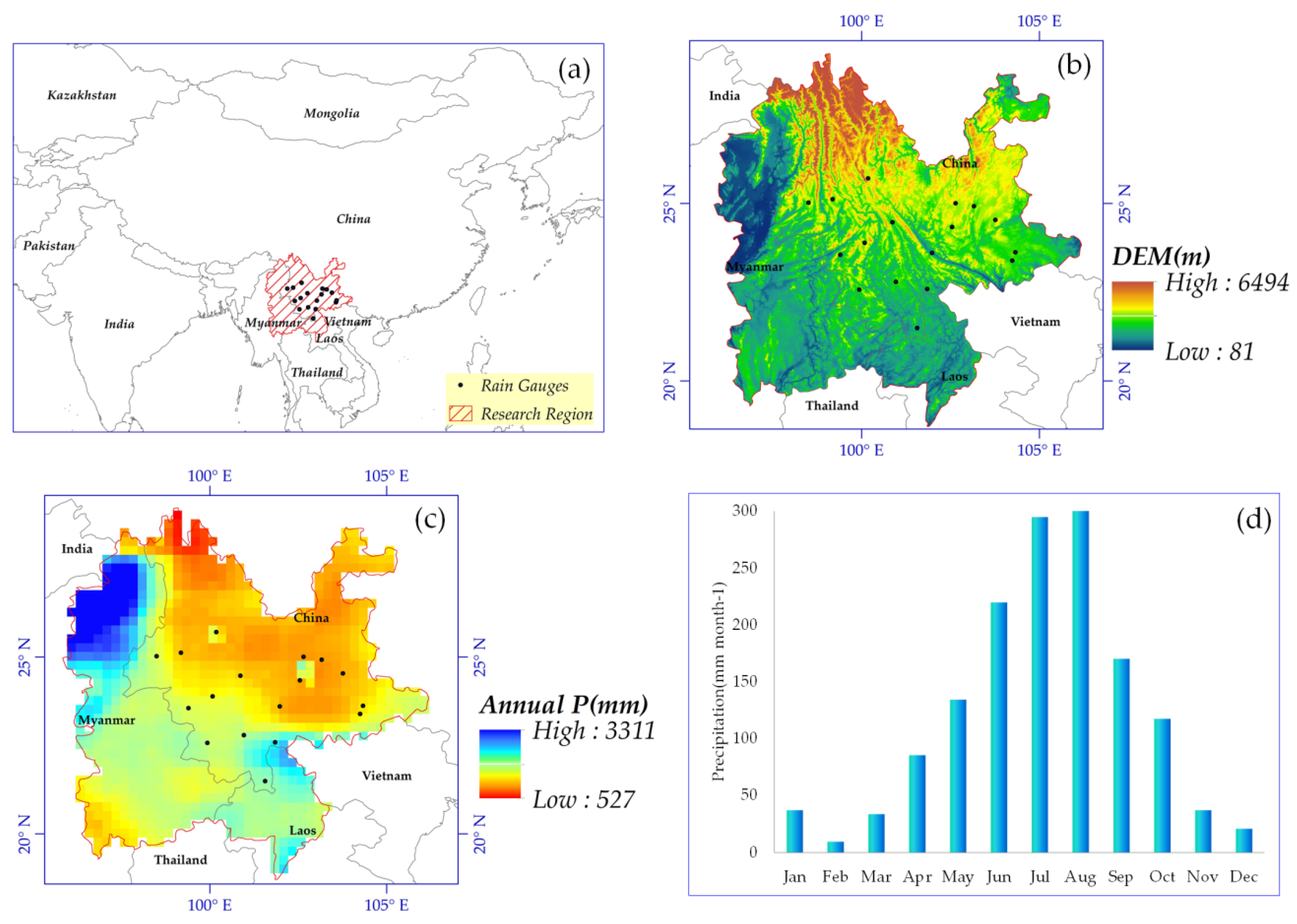
2.1. Study Area

The upstream area of the Great Mekong region, which has diverse vegetation and climate patterns and complex terrain, was selected as our study area. It extends from 95°50′18″E to 106°11′34″E and 29°13′20″N to 18°43′01″N, and approximately covers 692,379 km2 shared between China, Myanmar, and Laos (Figure 1a). Elevation decreases dramatically from 6494 m in the northwest to 81 m in the southeast with a north-south mountain-valley [51,52] (Figure 1b). The precipitation in this region is deeply affected by the complex seasonal monsoons [53], such as the southwest monsoon from the Indian Ocean and Bay of Bengal, resulting in an extremely uneven spatial and temporal distribution of precipitation. The average annual precipitation is 1494 mm yr−1, with the maximum annual precipitation of 3311 mm yr−1 in the Northern Myanmar and the minimum annual precipitation of 527 mm yr−1 in the Northwest Yunnan in China (Figure 1c). The temporal distribution of precipitation is also extremely uneven, the monthly average precipitation is approximately 122 mm month−1, and the minimum and maximum monthly precipitations are respectively 9 mm month−1 in February and 301 mm month−1 in August based on records from 2015 to 2018 (Figure 1d).

2.2. Data

This study used remote sensing precipitation (version 7 TRMM 3B43 dataset), vegetation indices (NDVI, EVI, and LAI), MCD12Q1 land cover dataset, and SRTM digital elevation model, (DEM). It should be highlighted that all these datasets are available on Google Earth Engine: https://developers.google.com/earth-engine/datasets. Moreover, this study also used monthly observed precipitation data from 17 weather stations provided by the China Meteorological Data Service Centre.

2.2.1. Precipitation

The Tropical Rainfall Measuring Mission was launched in 1997, which is a joint project by NASA and JAXA. The TRMM multi-satellite precipitation analysis (TMPA) was developed by combining several available satellite precipitation estimates, as well as with any possible precipitation gauge analyses [7]. One of TMPA products is the TRMM 3B43 monthly data with a 0.25° resolution. It is one of the most popular satellite-based precipitation datasets and has been widely used as the source data to downscale precipitation [1,10,24,33,54]. This study uses the TRMM 3B43 version 7 dataset, and it will be referred to as TRMM in subsequent sections.

2.2.2. Vegetation

The vegetation indices used in this study include the NDVI, EVI, and LAI. The NDVI and EVI are from the MOD13A2 version 6 dataset with low or no-clouds at 16-day composite and a 1 km spatial resolution. Many studies (Table A1) have used the vegetation index (e.g., NDVI and EVI) as a fundamental factor for downscaling precipitation because there is a positive correlation between it and precipitation. The LAI is collected from the MCD15A3H version 6 level 4 dataset. It is a 4-day composite dataset with a 500 m pixel size.

2.2.3. Land Cover

The MCD12Q1 Version 6 product provides annual global land cover at 500 m spatial resolution. MCD12Q1 is derived using supervised classifications of MODIS Terra and Aqua reflectance data and comes in five different classification schemes. The International Geosphere-Biosphere Programme (IGBP) classification scheme, which contains 17 land cover classes, was adopted for this study due to its broad applications [29,55].

2.2.4. Elevation

Previous studies have shown that elevation has a more substantial impact on precipitation in locations where the topography is not flat [10,54,56,57]. Considering the Shuttle Radar Topography Mission (SRTM, version 4) digital elevation dataset provides consistent, high-quality elevation data at a 90 m spatial resolution [58], so that this study adopts SRTM to investigate the effect of topography impact on precipitation patterns.

2.2.5. Rain Gauge

Since calibration with observed precipitation data is a crucial phase to improve the downscaled precipitation dataset, 17 monthly meteorological stations (Figure 1a) from the China Meteorological Data Service Centre are used to validate downscaled precipitation data. Most of the rain gauges are located in the central and eastern parts of China. The observation period is from January to December 2018. Generally, the study area is a sparse gauged area with only 17 rain gauges available.

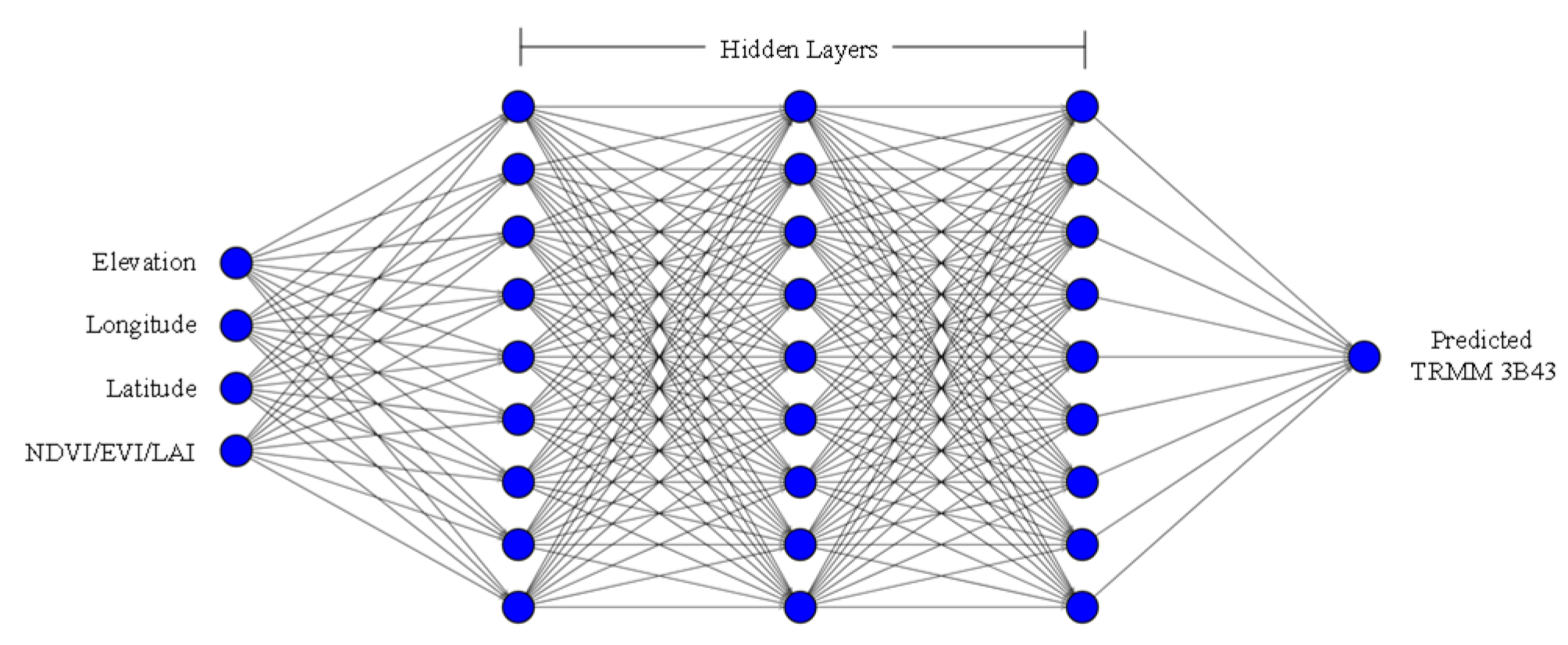
2.3. Machine Learning Algorithms

Three machine learning algorithms of the scikit-learn in Python [59] include the Gradient Boosting Regressor (GBR) [60], Support Vector Regression (SVR) [61], and Artificial Neural Network (ANN) [62] used to simulate the complicated relationship between TRMM precipitation and environmental factors for TRMM downscaling in this study. GBR is an ensemble learning algorithm that uses a boosting technique to minimize the loss of the model by adding weak learners in a stage-wise fashion. In each iterative step, a regression tree is fitted on a negative gradient (reduce the loss) of the given loss function and added to the model [63]. The final output from GBR is the ensemble of all the regression trees. The SVR relies on an optimization theory that uses a hyperplane to classify the input variables into an m-dimensional feature space with a maximal margin, which can be derived by solving a quadratic problem [61]. The ANN is an algorithm that interconnects processing units, called neurons or nodes, to each other as a network. This network can construct complex relationships between different sets of variables [64]. The ANN architecture consists of an input layer, at least one hidden layer, and an output layer. Each layer consists of several neurons. ANN has been successfully applied to downscale precipitation data [54,57,65]. In this study, the input layers number are four, which is equal to the number of independent variables (either NDVI, EVI, or LAI, Elevation, Longitude, and Latitude). The output layer is just one, which is the dependent variable (here, predicted TRMM) (Figure 2). The number of nodes within each hidden layer was 9. We calculate it by the following formula, the number of nodes= number of predictors * 2 + 1, which was proposed by Hecht-Nielsen [66].

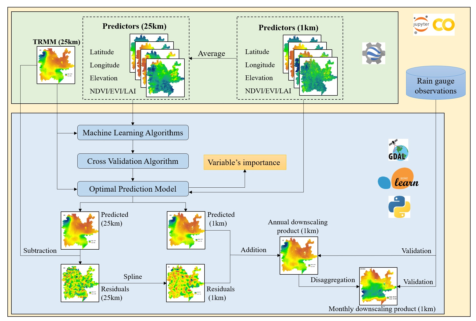
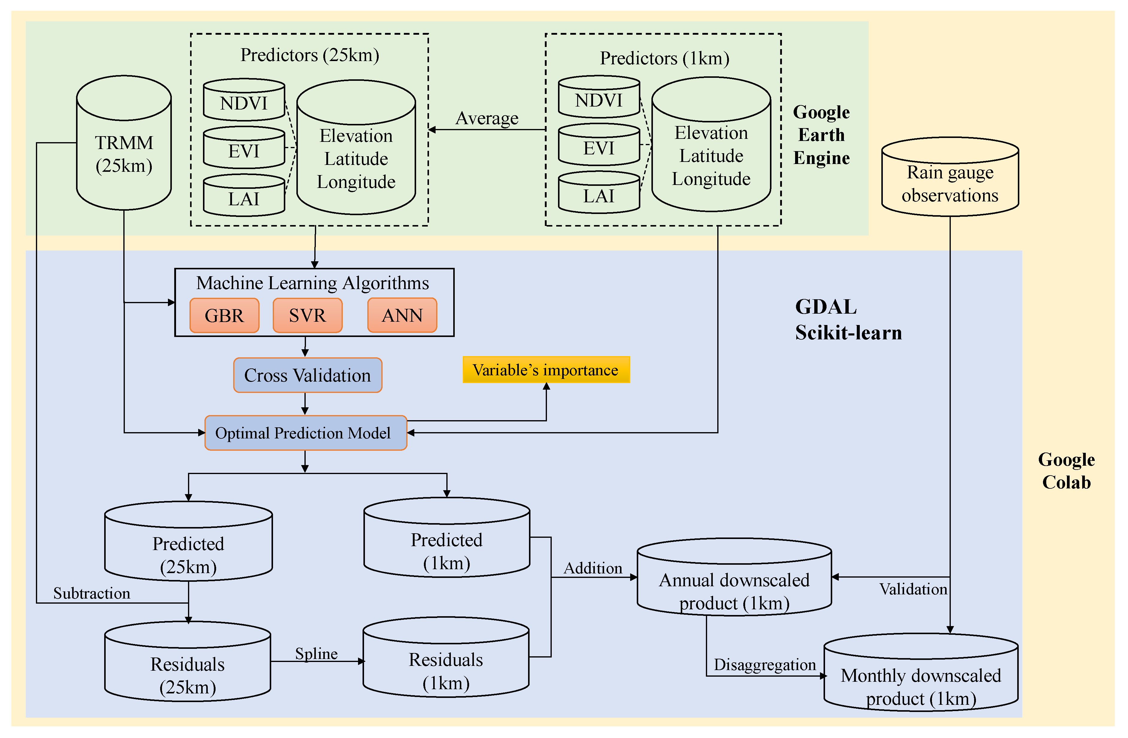
2.4. Downscaling Framework

The downscaling process can be expressed by P = F (Xi) + ε, where P is downscaled precipitation, Xi is environmental variables, ε is the residual. The general approach is to establish a correlation function (F) between precipitation and environmental variables at coarse resolution, and then use the fine-resolution environmental variable as inputs of F to predict precipitation at fine resolution. According to the study of Immerzeel, et al. [68], the function between predictors and TRMM precipitation is stable at coarse and fine resolution, only the coefficient has a smaller change, which means the model built on the coarse can be used at fine resolution.
According to the principle of the downscaling process and objectives of this study, an innovative downscaling framework (Figure 3) is designed by integrating GEE and three machine learning approaches using Google Colab. In this framework, the three machine learning algorithms are used to establish the relationship between precipitation and four environmental variables, including elevation, longitude, latitude, and one vegetation index (either NDVI, EVI, or LAI) ), and cross-validation is adopted to select the best downscaling algorithms. The best relationship between precipitation and environmental variables established at the coarse resolution (25 km) was applied to predict TRMM precipitation with 1 km resolution using 1 km environmental variables as an input. Except for monthly rain gauge data, other datasets, including TRMM, Elevation, Latitude, Longitude, NDVI, EVI, and LAI, are all processed online by GEE in Colab that avoids data downloading.

2.4.1. Data Preparation and Pre-Processing

Four environmental variables with a spatial resolution of 25 km and 1 km are prepared in this study, including three static variables (elevation, longitude, and latitude) and one dynamic variable (i.e., either NDVI, EVI, or LAI). In order to eliminate atmospheric and cloud cover effects, the maximum value composite was employed to generate the monthly dynamic variables. Then, the annual composite was generated by averaging the monthly values [25,27]. Environment variables at 25 km are generated by resampling the environment variables at 1 km using the nearest neighbor technique aggregated by the average of all 1 km pixels within each 25 km pixel [12]. All vegetation indices with negative values, as well as urban, built-up, permanent snow, ice, and water bodies of the MCD12Q1 land-use dataset, were masked out from both dependent and independent variables due to its negative impact on the construction of the downscaling model [10,12,29]. Because environment variables may differ in their ranges and units (i.e., NDVI/EVI, ranging from −1 to +1; LAI, ranging from 0.1 to 10; Elevation, ranging from 81 to 6494; Longitude, ranging from 95 to 106; Latitude, ranging from 18 to 29), the StandardScaler algorithm of scikit-learn was used to standardize variables using their means and standard deviation to eliminate the effects of different scaling [69].

2.4.2. Hyper-Parameter Optimization

The hyper-parameter of machine learning algorithms plays a pivotal role in its performance. In this framework, the scikit-learn GridSearchCV algorithm with cross-validation (GSCV) splitting strategy [59] is used to identify the best hyper-parameter values of each machine learning-vegetation index [12,35,70,71]. The total number of pixels at 25 km were divided into two groups. The first group constitutes 90%, and it is used for training and testing each algorithm to define the best hyper-parameters. For that, this study uses a 10-fold cross-validation strategy (CV = 10) to confirm the best hyper-parameters which construct the optimal prediction model (OPM). The remaining pixels at 25 km (10%) are used later to validate the OPM in simulating TRMM precipitation. The best OPM among the three survey models in this study was adopted to estimate the contribution of prediction variables in the downscaling model and downscale TRMM participation from 25 km to 1 km grids.

2.4.3. Generation of 1 km TRMM Product

Six steps are required to generate the final TRMM downscaling product with a resolution of 1 km [33,68]. Step 1: use the best OPM (established in Section 2.4.2) to predict TRMM at 25 km from the environmental variables at 25 km (Predicted (25 km)). Restricted by the regression model, there is an amount of precipitation that cannot be explained by the regression model [27,33,68]. Step 2: generate residual precipitation values with a resolution of 25 km using the following formula: ΔResidual (25 km) = TRMM (25 km) − Predicted (25 km). Step 3: resample the precipitation residual from 25 km to 1 km (ΔResidual (1 km)) using the spline algorithm [49] considering it works well for the regularly spaced data [35,54,57,70]. Step 4: use the same OPM used in Step 1 to generate TRMM prediction values with a resolution of 1 km by feeding the environmental variables at 1 km (Predicted (1 km)). Step 5: the final 1 km TRMM product is generated by the following equation: TRMM (1 km) = Predicted (1 km) + ΔResidual (1 km). Step 6: the annual TRMM downscaled at 1 km disaggregated into monthly precipitation maps following Duan and Bastiaanssen [27].

2.4.4. Assessment Indices

Three assessment indices (Equations (1)−(3)) were used to compare model performance [10,30], including the correlation of determination (R2), Root Mean Square Error (RMSE), and Mean Absolute Error (MAE).
R 2 = i = 1 n [ ( S i S ) ( P i P ¯ ) ] i = 1 n ( S i S ¯ ) 2   i = 1 n ( P i P ¯ ) 2    
RMSE = i = 1 n ( S i P i ) 2 n
MAE = i = 1 n | S i P i | n
where S is the original TRMM precipitation and P is the simulated TRMM precipitation. R2 is used to measure the strength of the relationship between the original and simulated precipitation [25], while MAE is used as a bias indicator, and RMSE is used to describe the accuracy of each machine learning algorithm [27]. In general, the higher R2 and the lower RMSE and MAE are the better the model. Besides, the analysis of variance (ANOVA) test was also applied to compare the performances of the investigated models in simulating TRMM precipitation [72]. The rain gauge data are used as ground “truth” to validate the final downscaled results; in this case: S is the observed precipitation and P is the downscaled TRMM precipitation.

3. Results

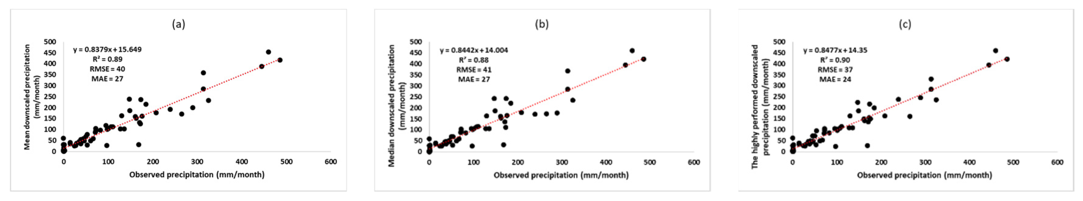
3.1. The Optimal Prediction Model

Table 1 shows the validation results of the simulated TRMM precipitation from different optimal prediction models. From Table 1, In general, the annual TRMM precipitation data predicted by the three machine learning methods show good consistency compared with the original TRMM data. ANN produced the highest R2 (ranges from 0.977 to 0.984) and the lowest RMSE (ranges from 71 mm year−1 to 85 mm year−1) and MAE (ranges from 51 mm year−1 to 56 mm year−1) in simulating TRMM annual precipitation, followed by GBR and SVR, respectively. The ANOVA analysis between the three algorithms (Table A2) revealed that there is a statistically significant difference among their performance in simulating TRMM precipitation (p-values < 0.05). Hence, in the following analysis, we employed ANN-based annual TRMM precipitation downscaling for the year 2018.

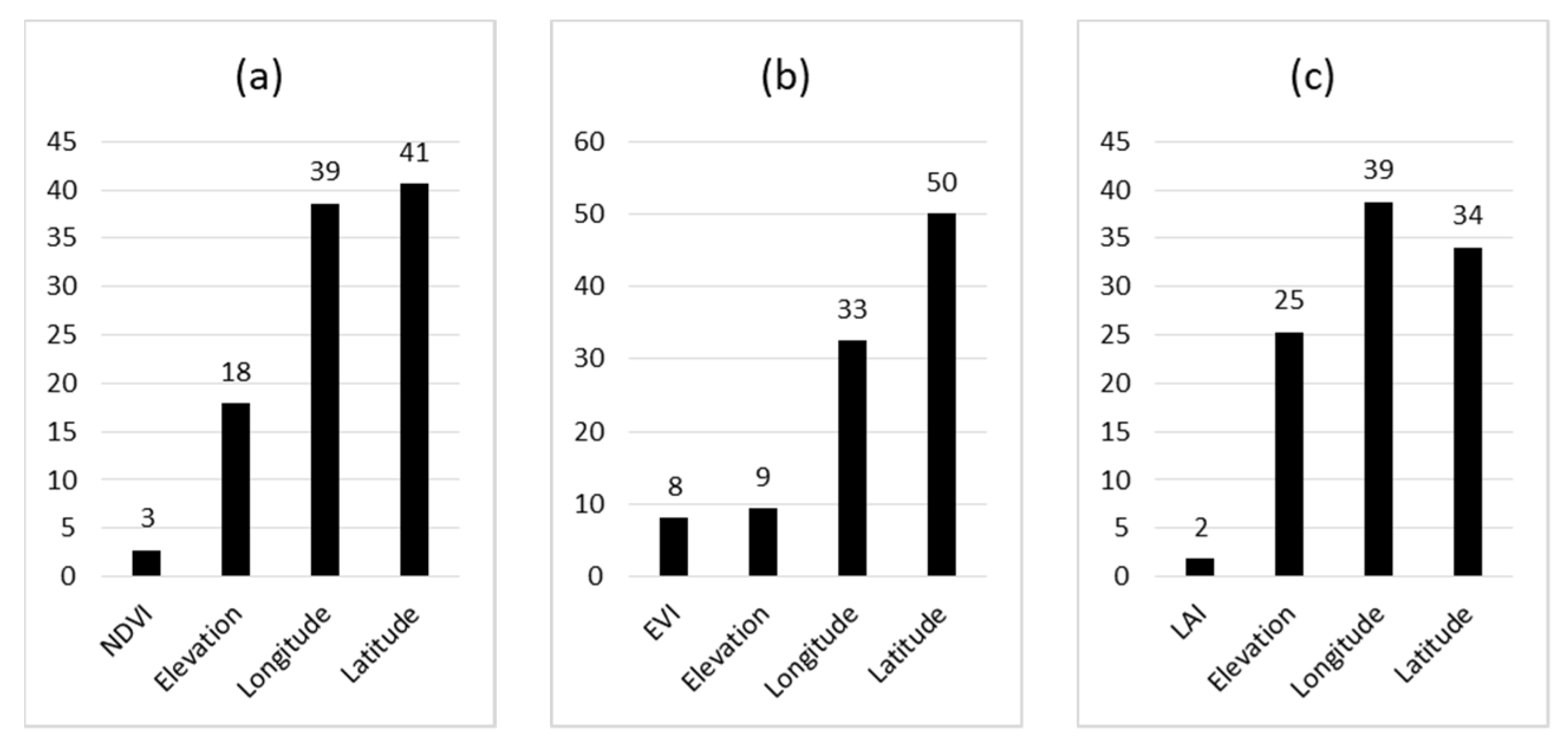
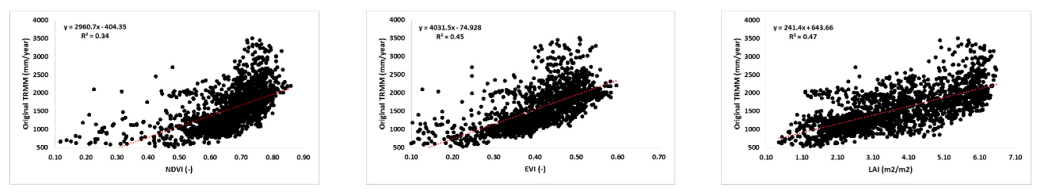
3.2. Variable Importance

The importance of input predictors for the ANN model (Figure 4) was identified by the scikit-learn “permutation importance” algorithm [73]. It reveals that latitude and longitude have the highest importance scores (34–50%), followed by elevation (9–25%), whereas vegetation indices, including EVI, NDVI, and LAI, contribute the last (2–8%). These findings are may because latitude and longitude as significant geolocation predictors play a dominant role in downscaling TRMM precipitation in the upstream area of the Great Mekong region. Among the three vegetation indices, EVI is the most crucial variable in contributing to the downscaling model flowed by NDVI and LAI.

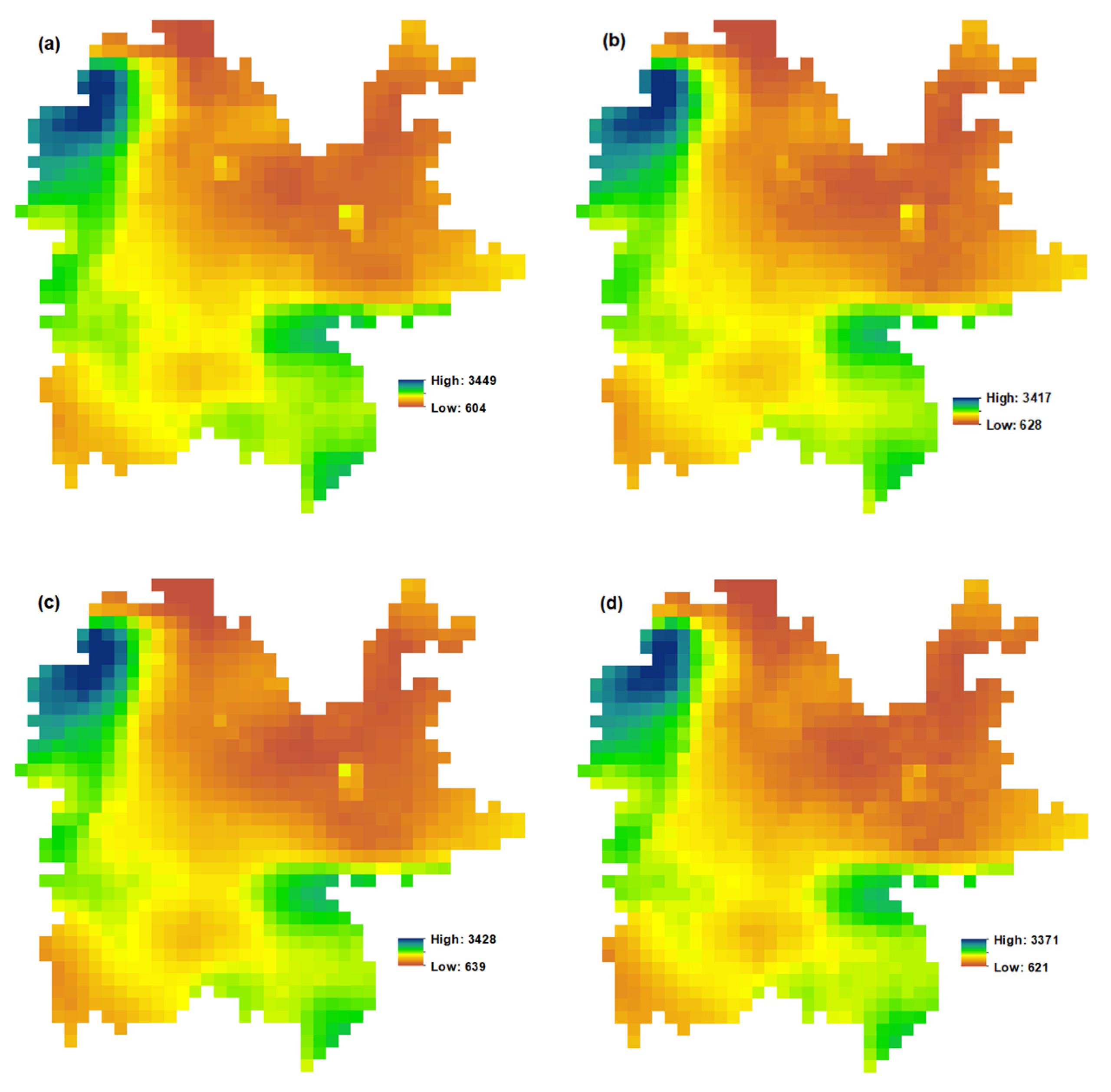
3.3. Annual Downscaled Products

Figure 5 presents the original TRMM precipitation and the predicted precipitation from the three different vegetation index for the year 2018 using the ANN algorithm. The predicted results share the same spatial pattern as the original TRMM precipitation. They are highly close regarding their means (a: 1558.12 mm year−1; b: 1556.46 mm year−1; c: 1556.36 mm year−1; d: 1555.31 mm year−1) but slightly differs in their spatial ranges. This also further proves the good performance of ANN in the TRMM precipitation forecast in 2018.
Figure 6 previews the residual precipitation maps at the coarse and fine resolutions. The residual maps represent the amount of precipitation that cannot be explained by the regression model. Negative values indicate areas where the independent variable effect is higher than expected (overestimation of the predicted precipitation). In contrast, positive values indicate areas where the independent variable effect is less than expected (underestimation of the predicted precipitation).
Figure 7 presents residuals precipitation contribution (RC) maps to the original TRMM and the downscaled precipitation before residual correction. RC values more than (0.5) 50% depict areas that the regression model is ineffective, and the downscaled result is mostly inherited from the residuals, which are not founded in the three predicted results. In this study, RC maps are classified into four classes (e.g., <0.05, 0.05–0.10, 0.10–0.20, >0.20) and then the contribution of each class (class cells number/total number of cells * 100) was calculated. Figure 7 reveals that a minor contribution of residuals in the downscaling model where the contribution of residuals less than 0.05 covers most of the study area; more than 83% of the total area at the coarse resolution and more than 93% of the total area at the fine resolution before residual correction.
Figure 8 presents the fine predicted precipitation before and after residual correction. In general, the downscaled results before and after residual correction have spatial distribution patterns similar to that of the original TRMM (Figure 5a), but with much more spatial variation and local details. The NDVI-predicted precipitation map before residual correction slightly has higher spatial precipitation patterns compared to the predicted precipitation using EVI and LAI datasets. After adding the residual precipitation, the spatial variation of NDVI-predicted precipitation becomes similar to other products (e.g., EVI and LAI). We compared the downscaled results after residual correction with the observed precipitation. The results show the R2, RMSE, and MAE were 0.91, 290 mm year−1, and 239 mm year−1 for NDVI-downscaled product, 0.89, 200 mm year−1, and 181 mm year−1 for EVI-downscaled product, and 0.91, 202 mm year−1, and 179 mm year−1 for the LAI-downscaled product, while those for the original TRMM precipitation were 0.79, 350 mm year−1, and 265 mm year−1.

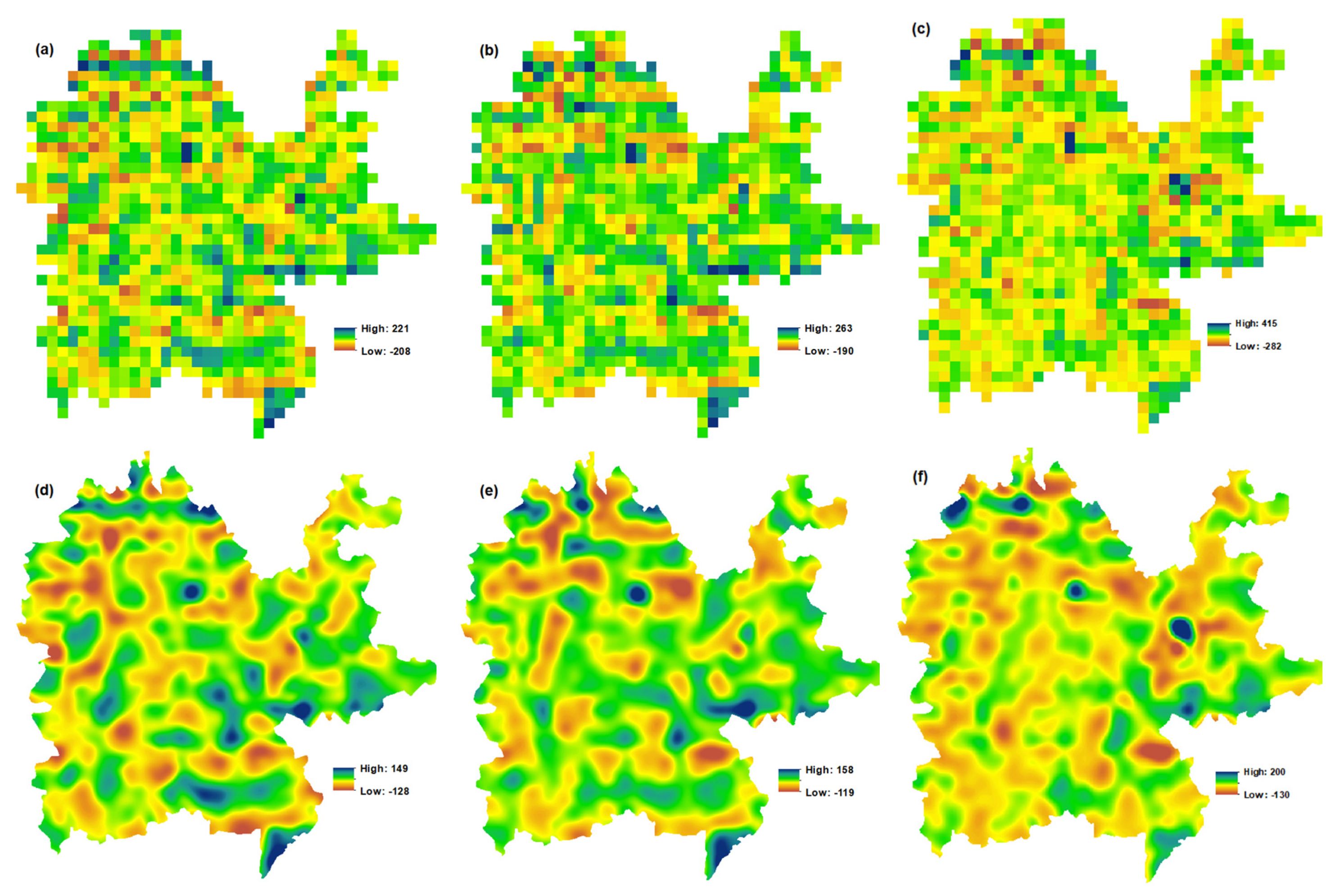
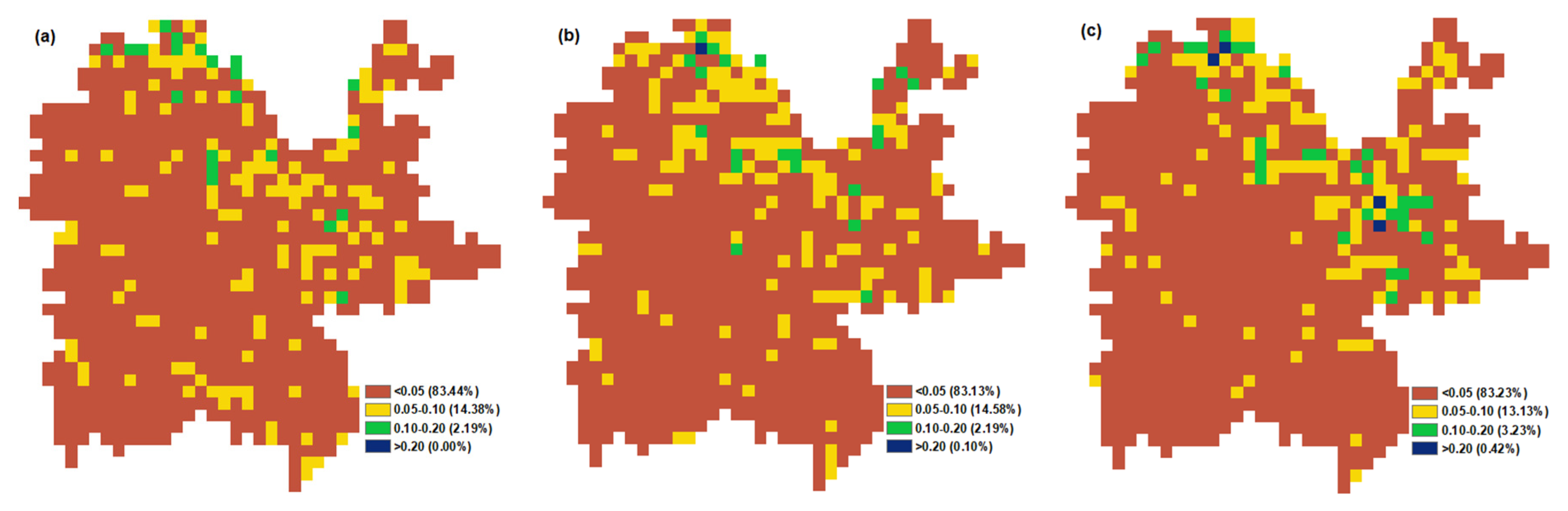
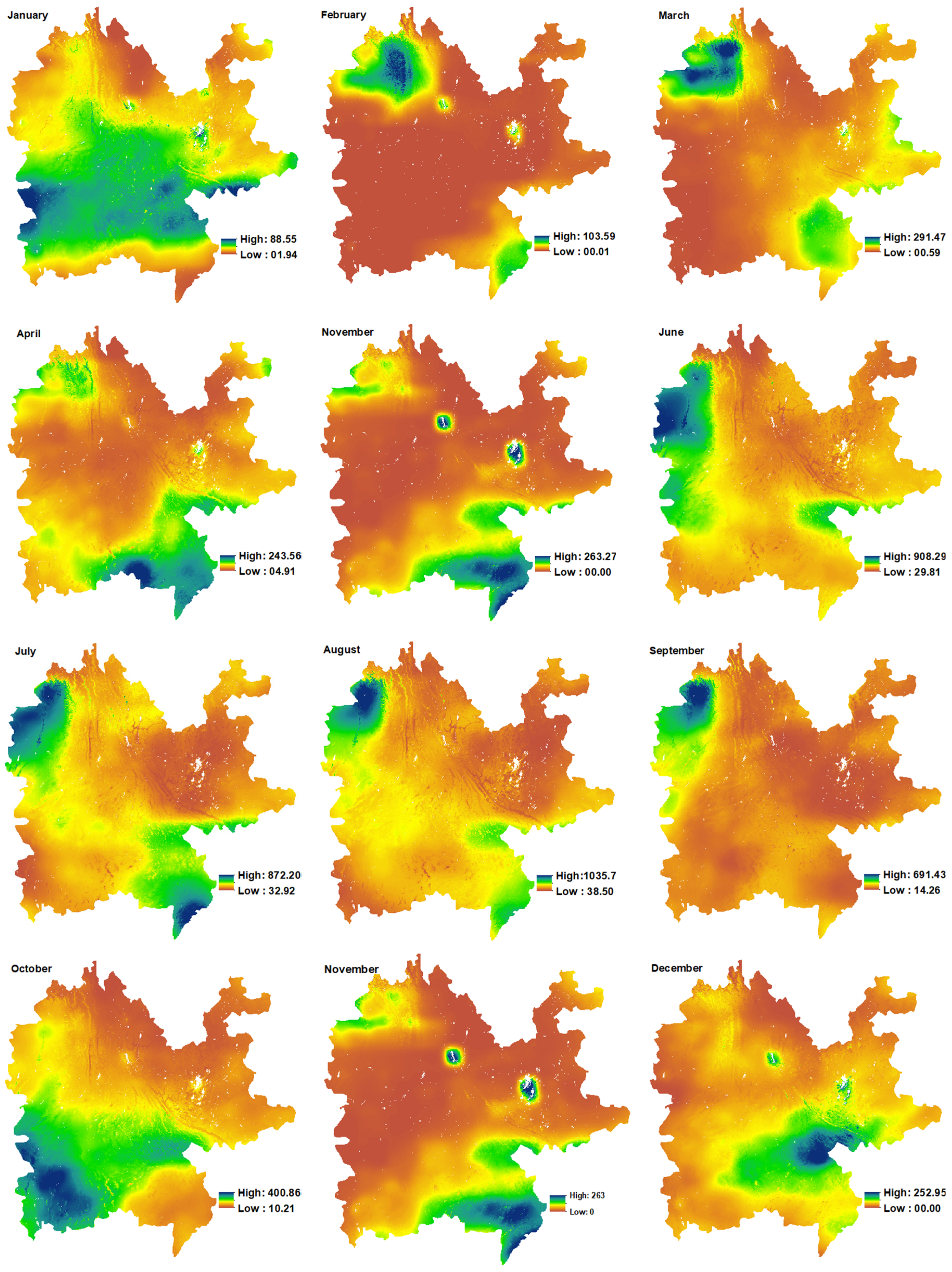
3.4. Monthly Downscaled Products

The monthly TRMM downscaled products are generated by decomposing the annual downscaled products for the year 2018. Figure 9 presents the validation metrics of the monthly downscaled products and the original TRMM precipitation versus the observed precipitation. In general, the three downscaled products returned a higher R2 and lower RMSE and MAE compared to the original TRMM precipitation. The LAI-downscaled results yielded the highest performance (R2 = 89, RMSE = 39 mm month−1, MAE = 27 mm month−1) followed by the EVI; the NDVI-downscaled product ranked the last.
There are three options regarding which product generated by each vegetation index may be used monthly: (1) the best product in all months (e.g., LAI); (2) the ensemble mean or median of the three products in each month; (3) the combination of the highly performed product from each month. Figure A1 proves that the last option outperforms the others (R2 = 90, RMSE = 37 mm month−1, MAE = 24 mm month−1). For that, the product that returned the highest R2 and the lowest RMSE and MAE was chosen to create the best combination of downscaling results for each month of the year 2018. More specifically, EVI-downscaled product is adopted in February, November, and December; NDVI-downscaled product is used in January, March, May, and September; while LAI-downscaled product is used in the remaining months. Compared with the original monthly TRMM data at 25 km spatial resolution (Figure 10), the downscaled maps at 1 km spatial resolution (Figure 11) present a similar overall precipitation pattern with more local details.

4. Discussion

Accurate precipitation data at high spatiotemporal resolution play an important role in land and water management. Downscaling coarse precipitation is an effective way to obtain precipitation estimates at a finer resolution for further essential environmental studies at the basin scale. In this study, we proposed a downscaling framework for TRMM precipitation products through integrating GEE and Colab. Three machine learning algorithms (GBR, SVR, and ANN) were investigated to simulate the TRMM precipitation data, and the highly performed algorithm used to derive the annual precipitation at a 1 km resolution over the Great Mekong region. Three vegetation indices (NDVI, EVI, and LAI) are compared in annual downscaling of TRMM and producing monthly maps of TRMM using disaggregation.

4.1. Result Compared to Previous Studies

Among the three algorithms that were implemented in this study, ANN performed the best in simulating the annual TRMM precipitation followed by GBR while SVR ranked the last. Our result is supported by Xu et al. [57], who found that ANN performs well in TRMM downscaling. However, there are different opinions on the performance of different machine learning methods. For example, Jing et al. [35] found that the performance of random forest is better than classification regression tree (CART) and KNN. In here, only one year of data was used in this study; we only provide an example to prove the applicability of the proposed framework in downscaling TRMM precipitation. Considering the relationship between these explanatory variables and precipitation is complex, the performance of different machine learning methods should be compared in practical applications.
The final annually downscaled maps (Figure 8d–f) show similar spatial precipitation patterns to the original precipitation (Figure 5a) with many local details. They also returned higher accuracies compared to the original TRMM when all compared against the observed precipitation (Figure 9). The highly performed downscaled product for each month is selected to consist of the downscaled TRMM of 1 km on a monthly scale (Figure 11). These maps compared to the original monthly TRMM precipitation (Figure 10) had similar overall spatial distributions but present a higher resolution and thus could display more detailed precipitation patterns. These results indicated that the downscaled precipitation in this study could improve not only the spatial resolution but also the accuracy of the TRMM downscaled precipitation. The findings are in accordance with previous results [24,57,68].
The effective of our framework is also proved by residual maps. In general, negative values of residual maps (e.g., greener areas) indicate that vegetation types in these areas may have an additional water source (e.g., irrigated areas) or it is less sensitive to precipitation (e.g., evergreen forest with deep rooting systems). On the other hand, positive values of residual maps may be characterized by vegetation types that are less green than would be expected (e.g., sparse vegetation). The higher residual magnitude returned by the LAI dataset followed by EVI, but these higher residuals are not dominant in the study area (Figure 6c). Figure 7 indicates that the three-predicted precipitation products present fewer residuals contribution to the downscaled precipitation.

4.2. Importance of Each Predictor and the Role of Vegetation Indices in TRMM Downscaling

Analysis of input variables importance in the downscaling which assigned by the ANN model indicated that latitude and longitude play a dominant role in downscaling TRMM precipitation in the study region. This result is in accordance with previous findings [29,57,74] that latitude and longitude may significantly affect precipitation and its spatial distribution. The higher importance score of elevation over all vegetation indices may be attributed to the uplift precipitation effects of mountains [10], in which case, the altitude affects the climate parameters that in turn influence the rate of precipitation [10,54,56]. Besides, the three vegetation indices were found to differ in their role in the downscaling model, where EVI introduced more contribution to the prediction model followed by NDVI while LAI produced the lower importance.
In general, the LAI-dataset performed slightly better than EVI, followed by NDVI in the annual downscaling model. This finding is may because the LAI dataset is found to be more correlated (R2 = 0.47) to precipitation than EVI (R2 = 0.45) and NDVI (R2 = 0.34), as shown in Figure A2. Another possible reason may be attributed to fine original spatiotemporal resolution of LAI (500 m; 4-days) compared to NDVI and EVI (1 km; 16-days). Furthermore, NDVI was reported by several studies [10,26,27,28,29] as prone to saturation when the precipitation exceeds a certain threshold. It is worth mentioning that LAI contributed fewer in terms of variable importance to the prediction model (Figure 4), but it performed the best in both annual and monthly downscaled products. This result indicates a higher importance score of a variable does not guarantee its better performance in precipitation downscaling. Alternatively, this study recommends the use of LAI to overcome both EVI and NDVI limitations, which may have neutralized the saturation effect.

4.3. Advantage and Disadvantage

The downscaling framework proposed by this study makes full use of the powerful data processing capabilities of Google Earth Engine and the powerful online computing capabilities of Google Cloud. It can help to achieve a deep coupling of online processing of remote sensing data and machine learning approaches. It does not require downloading data, installing software, and does not limit by personal computing devices. This framework allows easy comparison between different machine learning methods and is capable of selecting the optimal downscaling method and parameters based on specific regional characteristics. Despite that, this framework has some limitations. For example, it is limited by Google Drive space (15GB) and the Colab life cycle (12 h). Besides, the RAM and GPUs in Colab change with time to adapt to fluctuations in demand and the overall growth of user concurrent computing.

5. Conclusions

Accurate estimation of precipitation is a vital factor for land and water management application at the basin scale. The main merit of this framework is to deliver an easy to follow and accurate method for statistical downscaling TRMM precipitation by utilizing different sources of remote sensing data with machine learning methods, easy access, and a free processing environment. Python and GEE via Colab were used to facilitate the proposed downscaled procedures, which is time- and space-saving in data downloading, data format conversion, and data analysis. Three machine learning algorithms (GBR, SVR, and ANN) and auxiliary variables (elevation, latitude, longitude, and either NDVI, EVI, or LAI) were utilized to describe the relationship between precipitation and the geospatial environmental variables. Our results reveal that (1) the regression module based on ANN gave better and significant statistical metrics in simulating TRMM precipitation, (2) the most sensitive vegetation index for downscaling TRMM was the LAI followed by EVI, and (3) geolocation and elevation play an essential role in the downscaling model over the study area. The main conclusion of this study is that it is possible to accurately downscale TRMM precipitation which is a key input parameter in several essential studies [14,15,16,17,18,19,20,21,22,23] based on free-of-charge cloud computing. By this framework, the downscaling of TRMM precipitation can be achieved in a timely, efficient, and operational manner and the concept can be applied to another area for a similar subject as well as it is flexible to integrate more input variables and machine learning algorithms.

Author Contributions

A.E. was responsible for the experimental designing, manuscript preparation, and Jupyter notebook for data processing via Colab. H.Z. contributed to conceptual designing, editing, and reviewing the manuscript. B.W. contributed to the final reviewing of the manuscript, funding acquisition, and project administration, N.Z. contributed the structure designing, editing, and reviewing. F.T., M.Z., W.Z., N.Y., Z.C., Z.S., X.W., Y.L. gave useful comments which improved the paper. All authors have read and agreed to the published version of the manuscript.

Funding

This research was funded by the National Key R&D Program of China (2016YFA0600304, 2016YFA0600301), National Natural Science Foundation of China (41561144013, 41601464 and 41761144064), Key R&D project of Chinese Academy of Science (KFZD-SW-316), the environmental protection project of China Three Gorges Corporation.

Acknowledgments

Thanks to the China Meteorological Data Service Centre (CMDC) for providing the rain gauged precipitation data. Thanks to the Tropical Rainfall Measuring Mission (TRMM), the Moderate Resolution Imaging Spectroradiometer (MODIS) mission, and the Shuttle Radar Topography Mission (SRTM) for their data support. We would also like to thank all the staff members of the Python Software Foundation, Google Earth Engine, and Google Colab teams. Finally, we want to express our great appreciation to Anonymous reviewers and editors; your comments have significantly improved the quality of the article.

Conflicts of Interest

The authors declare no conflict of interest and no conflict of interest with China Three Gorges Corporation Company.

Source Code

Since the source code has been registered on the National Copyright of the People’s Republic of China (Certificate No: 5037633, Registration No: 2020SR0158937) as well as it relies on openly accessible sources, it can be shared by emailing the correspondence author.

Appendix A

Table A1. Summary of relevant studies for monthly downscaling TRMM precipitation data.
ReferencePredictorsResidual
correction
Regression
model
Performance
R2RMSEMAE
(mm month−1)
[34] *DEM, aspect, roughness, humidity, temperatureSplineMLR0.5819.99--
TRMM0.5839.45--
[24]NDVI, DEMArea-to-point KrigingMLR--20.0313.03
Ordinary Kriging--24.8117.73
[57]DEM, Long, LatSplineANN0.93640.56--
MF0.93441.20--
[74]NDVI, LST, DEM, slope, Long, LatOrdinary KrigingGWRK0.952516
TRMM0.953019
[75]EVI, DEM, aspect, slope, Long, LatBilinearRF0.782514
TRMM0.733116
[54]NDVI, VWSI,
albedo, DEM,
SplineMLR0.4754--
ANN0.6059--
TRMM--37--
[76]NDVI, DEM, LST-SVM0.7529.90--
RF0.8226.10--
[35]NDVI, DEM, LSTSplineMLR0.462714
kNN0.711712
CART0.701812
SVM0.731611
RF0.741611
[29] **NDVI, DEM,
slope, Long, Lat
KrigingGWRK0.9122.213.5
0.847.504.8
0.8030.522.2
TRMM0.8826.513.7
--5.103.8
0.6937.123.7
[25] ***NDVI, DEMBilinearExponential0.7424--
0. 6025
GWR0.6732--
0.4220
MLR0.8022--
0.2615
QPP0.8916--
0.4511
TRMM0.9411--
0.649--
[77]DEM, Long, Lat, TRMM-1 km-GWR0.8732.9218.19
Ordinary KrigingGWRK0.8931.1117.05
TRMM downscaled by ATPK to 1 km (TRMM-1 km)0.7646.1426.44
TRMM0.7249.6328.66
[30]EVI, DEM--GWR------
NDVI, DEM0.863523
TRMM0.853826
Note: Geographically Weighted Regression Kriging (GWRK); Geographically Weighted Regression (GWR); Area-to-point Kriging (ATPK); Optimal Subset Regression (OSR); Multiple Linear Regression (MLR); Artificial Neural Network (ANN); Multi-fractal approach (MF); Vegetation Water Supply Index (VWSI), Land Surface Temperature (LST), Random Forest (RF); Quadratic Parabolic Profile (QPP); Classification and Regression Trees (CART); Cubist is a spatial data mining algorithm; Longitude (Long); Latitude (Lat). * R2 and RMSE values represent the mean for the six events, ** performance during monthly (higher row), dry season (middle row), and wet season (lower row), *** performance using national stations (higher row) and regional stations (lower row).

Appendix B

Table A2. Summary of ANOVA analysis test between the investigated algorithms performance in simulating TRMM precipitation for the year 2018.
MetricsSource of VariationSSdfMSFp-ValueF crit
R2Between Groups0.000820.00038200.0025.14
Within Groups0.000160.00002
Total0.00098
RMSEBetween Groups206921035220.0025.14
Within Groups286648
Total23558
MAEBetween Groups7282364720.00015.14
Within Groups3065
Total7588
Note: SS: Sum-of-Squares; df: the degree of freedom; MS: Mean Square; F: F test statistic; p-value: probability value (here it is at 0.05); F crit: F critical value.

Appendix C

Figure A1. Monthly validation results of the ensemble mean (a), ensemble median (b), and the highly performed (c) monthly downscaled TRMM by disaggregation using ANN algorithm and NDVI, EVI, and LAI vegetation indices, 2018.
Remotesensing 12 03860 g0a1

Appendix D

Figure A2. Mean annual values of NDVI, EVI, and LAI versus the original TRMM for the year 2018.
Remotesensing 12 03860 g0a2

References

  1. Zhang, Z.; Tian, J.; Huang, Y.; Chen, X.; Chen, S.; Duan, Z. Hydrologic evaluation of TRMM and GPM IMERG Satellite-Based precipitation in a Humid Basin of China. Remote Sens. 2019, 11, 431. [Google Scholar] [CrossRef] [Green Version]
  2. Luo, X.; Wu, W.; He, D.; Li, Y.; Ji, X. Hydrological simulation using TRMM and CHIRPS precipitation estimates in the Lower Lancang-Mekong River Basin. Chin. Geogr. Sci. 2019, 29, 13–25. [Google Scholar] [CrossRef] [Green Version]
  3. Kubota, T.; Shige, S.; Hashizume, H.; Aonashi, K.; Takahashi, N.; Seto, S.; Hirose, M.; Takayabu, Y.N.; Ushio, T.; Nakagawa, K.; et al. Global Precipitation Map Using Satellite-Borne Microwave Radiometers by the GSMaP Project: Production and Validation. IEEE Trans. Geosci. Remote Sens. 2007, 45, 2259–2275. [Google Scholar] [CrossRef]
  4. Funk, C.; Peterson, P.; Landsfeld, M.; Pedreros, D.; Verdin, J.; Shukla, S.; Husak, G.; Rowland, J.; Harrison, L.; Hoell, A. The climate hazards infrared precipitation with stations-a new environmental record for monitoring extremes. Sci. Data 2015, 2, 150066. [Google Scholar] [CrossRef] [Green Version]
  5. Ashouri, H.; Hsu, K.-L.; Sorooshian, S.; Braithwaite, D.K.; Knapp, K.R.; Cecil, L.D.; Nelson, B.R.; Prat, O.P. PERSIANN-CDR: Daily Precipitation Climate Data Record from Multisatellite Observations for Hydrological and Climate Studies. Bull. Am. Meteorol. Soc. 2015, 96, 69–83. [Google Scholar] [CrossRef] [Green Version]
  6. Yamamoto, M.K.; Shige, S. Implementation of an orographic/nonorographic rainfall classification scheme in the GSMaP algorithm for microwave radiometers. Atmos. Res. 2015, 163, 36–47. [Google Scholar] [CrossRef]
  7. Huffman, G.J.; Bolvin, D.T.; Nelkin, E.J.; Wolff, D.B.; Adler, R.F.; Gu, G.; Hong, Y.; Bowman, K.P.; Stocker, E.F. The TRMM Multisatellite Precipitation Analysis (TMPA): Quasi-global, multiyear, combined-sensor precipitation estimates at fine scales. J. Hydrometeorol. 2007, 8, 38–55. [Google Scholar] [CrossRef]
  8. Zeng, H.; Wu, B.; Zhang, N.; Tian, F.; Phiri, E.; Musakwa, W.; Zhang, M.; Zhu, L.; Mashonjowa, E. Spatiotemporal Analysis of Precipitation in the Sparsely Gauged Zambezi River Basin Using Remote Sensing and Google Earth Engine. Remote Sens. 2019, 11, 2977. [Google Scholar] [CrossRef] [Green Version]
  9. Zhou, Z.; Guo, B.; Su, Y.; Chen, Z.; Wang, J. Multidimensional evaluation of the TRMM 3B43V7 satellite-based precipitation product in mainland China from 1998–2016. PeerJ 2020, 8, e8615. [Google Scholar] [CrossRef] [Green Version]
  10. Shi, Y.; Song, L.; Xia, Z.; Lin, Y.; Myneni, R.B.; Choi, S.; Wang, L.; Ni, X.; Lao, C.; Yang, F. Mapping annual precipitation across Mainland China in the Period 2001–2010 from TRMM3B43 product using spatial downscaling approach. Remote Sens. 2015, 7, 5849. [Google Scholar] [CrossRef] [Green Version]
  11. Adhikary, S.K.; Yilmaz, A.G.; Muttil, N. Optimal design of rain gauge network in the Middle Yarra River catchment, Australia. Hydrol. Process. 2015, 29, 2582–2599. [Google Scholar] [CrossRef] [Green Version]
  12. Jing, W.; Yang, Y.; Yue, X.; Zhao, X. A Spatial Downscaling Algorithm for Satellite-Based Precipitation over the Tibetan Plateau Based on NDVI, DEM, and Land Surface Temperature. Remote Sens. 2016, 8, 655. [Google Scholar] [CrossRef] [Green Version]
  13. Ulloa, J.; Ballari, D.; Campozano, L.; Samaniego, E. Two-Step Downscaling of TRMM 3B43 V7 Precipitation in Contrasting Climatic Regions with Sparse Monitoring: The Case of Ecuador in Tropical South America. Remote Sens. 2017, 9, 758. [Google Scholar] [CrossRef] [Green Version]
  14. Weltzin, J.F.; Loik, M.E.; Schwinning, S.; Williams, D.G.; Fay, P.A.; Haddad, B.M.; Harte, J.; Huxman, T.E.; Knapp, A.K.; Lin, G.; et al. Assessing the Response of Terrestrial Ecosystems to Potential Changes in Precipitation. BioScience 2003, 53, 941–952. [Google Scholar] [CrossRef]
  15. Potts, D.L.; Barron-Gafford, G.A.; Butterfield, B.J.; Fay, P.A.; Hultine, K.R. Bloom and Bust: Ecological consequences of precipitation variability in aridlands. Plant Ecol. 2019, 220, 135–139. [Google Scholar] [CrossRef] [Green Version]
  16. Oki, T.; Kanae, S. Global hydrological cycles and world water resources. Science 2006, 313, 1068–1072. [Google Scholar] [CrossRef] [Green Version]
  17. Trenberth, K.E.; Smith, L.; Qian, T.; Dai, A.; Fasullo, J. Estimates of the Global Water Budget and Its Annual Cycle Using Observational and Model Data. J. Hydrometeorol. 2007, 8, 758–769. [Google Scholar] [CrossRef]
  18. Rodell, M.; Beaudoing, H.K.; L’Ecuyer, T.S.; Olson, W.S.; Famiglietti, J.S.; Houser, P.R.; Adler, R.; Bosilovich, M.G.; Clayson, C.A.; Chambers, D.; et al. The Observed State of the Water Cycle in the Early Twenty-First Century. J. Clim. 2015, 28, 8289–8318. [Google Scholar] [CrossRef]
  19. Yang, X.; Chen, R.; Meadows, M.E.; Ji, G.; Xu, J. Modelling water yield with the InVEST model in a data scarce region of northwest China. Water Supply 2020, 20, 1035–1045. [Google Scholar] [CrossRef]
  20. López López, P.; Immerzeel, W.W.; Rodríguez Sandoval, E.A.; Sterk, G.; Schellekens, J. Spatial Downscaling of Satellite-Based Precipitation and Its Impact on Discharge Simulations in the Magdalena River Basin in Colombia. Front. Earth Sci. 2018, 6. [Google Scholar] [CrossRef] [Green Version]
  21. Dutta, D.; Das, S.; Kundu, A.; Taj, A. Soil erosion risk assessment in Sanjal watershed, Jharkhand (India) using geo-informatics, RUSLE model and TRMM data. Model. Earth Syst. Environ. 2015, 1, 37. [Google Scholar] [CrossRef]
  22. Teng, H.; Ma, Z.; Chappell, A.; Shi, Z.; Liang, Z.; Yu, W. Improving Rainfall Erosivity Estimates Using Merged TRMM and Gauge Data. Remote Sens. 2017, 9, 1134. [Google Scholar] [CrossRef] [Green Version]
  23. Phinzi, K.; Ngetar, N.S. The assessment of water-borne erosion at catchment level using GIS-based RUSLE and remote sensing: A review. Int. Soil Water Conserv. Res. 2019, 7, 27–46. [Google Scholar] [CrossRef]
  24. Park, N.-W. Spatial downscaling of TRMM precipitation using geostatistics and fine scale environmental variables. Adv. Meteorol. 2013, 2013, 237126. [Google Scholar] [CrossRef]
  25. Zhang, T.; Li, B.; Yuan, Y.; Gao, X.; Sun, Q.; Xu, L.; Jiang, Y. Spatial downscaling of TRMM precipitation data considering the impacts of macro-geographical factors and local elevation in the Three-River Headwaters Region. Remote Sens. Environ. 2018, 215, 109–127. [Google Scholar] [CrossRef]
  26. Quiroz, R.; Yarlequé, C.; Posadas, A.; Mares, V.; Immerzeel, W.W. Improving daily rainfall estimation from NDVI using a wavelet transform. Environ. Model. Softw. 2011, 26, 201–209. [Google Scholar] [CrossRef]
  27. Duan, Z.; Bastiaanssen, W.G.M. First results from version 7 TRMM 3B43 precipitation product in combination with a new downscaling-calibration procedure. Remote Sens. Environ. 2013, 131, 1–13. [Google Scholar] [CrossRef]
  28. Liu, J.; Zhang, W.; Nie, N. Spatial Downscaling of TRMM precipitation data using an optimal subset regression model with NDVI and terrain factors in the Yarlung Zangbo River Basin, China. Adv. Meteorol. 2018, 2018, 3491960. [Google Scholar] [CrossRef]
  29. Zhang, Y.; Li, Y.; Ji, X.; Luo, X.; Li, X. Fine-resolution precipitation mapping in a mountainous watershed: Geostatistical downscaling of TRMM products based on environmental variables. Remote Sens. 2018, 10, 119. [Google Scholar] [CrossRef] [Green Version]
  30. Chen, S.; Zhang, L.; She, D.; Chen, J. Spatial downscaling of Tropical Rainfall Measuring Mission (TRMM) annual and monthly precipitation data over the Middle and Lower Reaches of the Yangtze River Basin, China. Water 2019, 11, 568. [Google Scholar] [CrossRef] [Green Version]
  31. Maki, M.; Homma, K. Empirical Regression Models for Estimating Multiyear Leaf Area Index of Rice from Several Vegetation Indices at the Field Scale. Remote Sens. 2014, 6, 4764–4779. [Google Scholar] [CrossRef] [Green Version]
  32. Din, M.; Zheng, W.; Rashid, M.; Wang, S.; Shi, Z. Evaluating hyperspectral vegetation indices for leaf area index estimation of Oryza sativa L. at diverse phenological stages. Front. Plant Sci. 2017, 8, 820. [Google Scholar] [CrossRef] [PubMed] [Green Version]
  33. Jia, S.; Zhu, W.; Lű, A.; Yan, T. A statistical spatial downscaling algorithm of TRMM precipitation based on NDVI and DEM in the Qaidam Basin of China. Remote Sens. Environ. 2011, 115, 3069–3079. [Google Scholar] [CrossRef]
  34. Fang, J.; Du, J.; Xu, W.; Shi, P.; Li, M.; Ming, X. Spatial downscaling of TRMM precipitation data based on the orographical effect and meteorological conditions in a mountainous area. Adv. Water Resour. 2013, 61, 42–50. [Google Scholar] [CrossRef]
  35. Jing, W.; Yang, Y.; Yue, X.; Zhao, X. A Comparison of Different Regression Algorithms for Downscaling Monthly Satellite-Based Precipitation over North China. Remote Sens. 2016, 8, 835. [Google Scholar] [CrossRef] [Green Version]
  36. Gorelick, N.; Hancher, M.; Dixon, M.; Ilyushchenko, S.; Thau, D.; Moore, R. Google Earth Engine: Planetary-scale geospatial analysis for everyone. Remote Sens. Environ. 2017, 202, 18–27. [Google Scholar] [CrossRef]
  37. Kumar, L.; Mutanga, O. Google Earth Engine applications since inception: Usage, trends, and potential. Remote Sens. 2018, 10, 1509. [Google Scholar] [CrossRef] [Green Version]
  38. Lobell, D.B.; Thau, D.; Seifert, C.; Engle, E.; Little, B. A scalable satellite-based crop yield mapper. Remote Sens. Environ. 2015, 164, 324–333. [Google Scholar] [CrossRef]
  39. Shelestov, A.; Lavreniuk, M.; Kussul, N.; Novikov, A.; Skakun, S. Exploring Google Earth Engine platform for big data processing: Classification of multi-temporal satellite imagery for crop mapping. Front. Earth Sci. 2017, 5. [Google Scholar] [CrossRef] [Green Version]
  40. Mandal, D.; Kumar, V.; Bhattacharya, A.; Rao, Y.S.; Siqueira, P.; Bera, S. Sen4Rice: A Processing Chain for Differentiating Early and Late Transplanted Rice Using Time-Series Sentinel-1 SAR Data with Google Earth Engine. IEEE Geosci. Remote Sens. Lett. 2018, 15, 1947–1951. [Google Scholar] [CrossRef]
  41. Tian, F.; Wu, B.; Zeng, H.; Zhang, X.; Xu, J. Efficient identification of corn cultivation area with multitemporal synthetic aperture radar and optical images in the Google Earth Engine cloud platform. Remote Sens. 2019, 11, 629. [Google Scholar] [CrossRef] [Green Version]
  42. Long, T.; Zhang, Z.; He, G.; Jiao, W.; Tang, C.; Wu, B.; Zhang, X.; Wang, G.; Yin, R. 30 m resolution global annual burned area mapping based on Landsat images and Google Earth Engine. Remote Sens. 2019, 11, 489. [Google Scholar] [CrossRef] [Green Version]
  43. Alonso, A.; Muñoz-Carpena, R.; Kennedy, R.E.; Murcia, C. Wetland landscape spatio-temporal degradation dynamics using the new Google Earth Engine cloud-based platform: Opportunities for non-specialists in remote sensing. Am. Soc. Agric. Biol. Eng. 2016, 59, 1331–1342. [Google Scholar] [CrossRef] [Green Version]
  44. Tsai, Y.H.; Stow, D.; Chen, H.L.; Lewison, R.; An, L.; Shi, L. Mapping Vegetation and Land Use Types in Fanjingshan National Nature Reserve Using Google Earth Engine. Remote Sens. 2018, 10, 927. [Google Scholar] [CrossRef] [Green Version]
  45. Mahdianpari, M.; Salehi, B.; Mohammadimanesh, F.; Homayouni, S.; Gill, E. The first wetland inventory map of Newfoundland at a spatial resolution of 10 m using Sentinel-1 and Sentinel-2 data on the Google Earth Engine cloud computing platform. Remote Sens. 2018, 11, 43. [Google Scholar] [CrossRef] [Green Version]
  46. Zhang, Y.; Kong, D.; Gan, R.; Chiew, F.H.S.; McVicar, T.R.; Zhang, Q.; Yang, Y. Coupled estimation of 500m and 8-day resolution global evapotranspiration and gross primary production in 2002–2017. Remote Sens. Environ. 2019, 222, 165–182. [Google Scholar] [CrossRef]
  47. Foolad, F.; Blankenau, P.; Kilic, A.; Allen, R.G.; Huntington, J.L.; Erickson, T.A.; Ozturk, D.; Morton, C.G.; Ortega, S.; Ratcliffe, I. Comparison of the automatically calibrated Google evapotranspiration application-EEFlux and the manually calibrated METRIC application. Preprints 2018, 2018070040. [Google Scholar] [CrossRef]
  48. Carneiro, T.; Da Nóbrega, R.V.M.; Nepomuceno, T.; Bian, G.-B.; De Albuquerque, V.H.C.; Filho, P.P.R. Performance analysis of Google Colaboratory as a tool for accelerating deep learning applications. IEEE Access 2018, 6, 61677–61685. [Google Scholar] [CrossRef]
  49. Warmerdam, F. The Geospatial Data Abstraction Library. In Open Source Approaches in Spatial Data Handling; Hall, G.B., Leahy, M.G., Eds.; Springer: Berlin/Heidelberg, Germany, 2008; pp. 87–104. [Google Scholar] [CrossRef]
  50. Bisong, E. Google Colaboratory. In Building Machine Learning and Deep Learning Models on Google Cloud Platform: A Comprehensive Guide for Beginners; Bisong, E., Ed.; Apress: Berkeley, CA, USA, 2019; pp. 59–64. [Google Scholar] [CrossRef]
  51. Wu, F.; Wang, X.; Cai, Y.; Li, C. Spatiotemporal analysis of precipitation trends under climate change in the upper reach of Mekong River basin. Quat. Int. 2016, 392, 137–146. [Google Scholar] [CrossRef] [Green Version]
  52. Li, Z.; He, Y.; Wang, C.; Wang, X.; Xin, H.; Zhang, W.; Cao, W. Spatial and temporal trends of temperature and precipitation during 1960–2008 at the Hengduan Mountains, China. Quat. Int. 2011, 236, 127–142. [Google Scholar] [CrossRef]
  53. Xiao, X.Y.; Shen, J.; Wang, S.M.; Xiao, H.F.; Tong, G.B. The variation of the southwest monsoon from the high resolution pollen record in Heqing Basin, Yunnan Province, China for the last 2.78Ma. Palaeogeogr. Palaeoclimatol. Palaeoecol. 2010, 287, 45–57. [Google Scholar] [CrossRef]
  54. Alexakis, D.D.; Tsanis, I.K. Comparison of multiple linear regression and artificial neural network models for downscaling TRMM precipitation products using MODIS data. Environ. Earth Sci. 2016, 75, 1077. [Google Scholar] [CrossRef]
  55. Fan, D.; Wu, H.; Dong, G.; Jiang, X.; Xue, H. A Temporal Disaggregation Approach for TRMM Monthly Precipitation Products Using AMSR2 Soil Moisture Data. Remote Sens. 2019, 11, 2962. [Google Scholar] [CrossRef] [Green Version]
  56. Hunink, J.E.; Immerzeel, W.W.; Droogers, P. A High-resolution Precipitation 2-step mapping Procedure (HiP2P): Development and application to a tropical mountainous area. Remote Sens. Environ. 2014, 140, 179–188. [Google Scholar] [CrossRef]
  57. Xu, G.; Xu, X.; Liu, M.; Sun, A.Y.; Wang, K. Spatial downscaling of TRMM precipitation product using a combined multifractal and regression approach: Demonstration for South China. Water 2015, 7, 3083. [Google Scholar] [CrossRef] [Green Version]
  58. Jarvis, A.; Reuter, H.I.; Nelson, A.; Guevara, E. Hole-Filled SRTM for the Globe Version 4, Available from the CGIAR-CSI SRTM 90 m. 2008. Available online: http://srtm.csi.cgiar.org (accessed on 23 January 2020).
  59. Pedregosa, F.; Varoquaux, G.; Gramfort, A.; Thirion, B.; Michel, V.; Grisel, O.; Blondel, M.; Prettenhofer, P.; Weiss, R.; Dubourg, V.; et al. Scikit-learn: Machine Learning in Python. J. Mach. Learn. Res. 2011, 12, 2825–2830. [Google Scholar]
  60. Friedman, J.H. Stochastic gradient boosting. Comput. Stat. Data Anal. 2002, 38, 367–378. [Google Scholar] [CrossRef]
  61. Smola, A.J.; Schölkopf, B. A tutorial on support vector regression. Stat. Comput. 2004, 14, 199–222. [Google Scholar] [CrossRef] [Green Version]
  62. Specht, D.F. A general regression neural network. IEEE Trans. Neural Netw. 1991, 2, 568–576. [Google Scholar] [CrossRef] [Green Version]
  63. Friedman, J.H. Greedy Function Approximation: A Gradient Boosting Machine. Ann. Stat. 2001, 29, 1189–1232. [Google Scholar] [CrossRef]
  64. Hinton, G.E. Connectionist learning procedures. Artif. Intell. 1989, 40, 185–234. [Google Scholar] [CrossRef] [Green Version]
  65. Kumar, R.; Das, I.; Gairola, R.; Sarkar, A.; Agarwal, V.K. Rainfall retrieval from TRMM radiometric channels using artificial neural networks. Indian J. Radio Space Phys. 2007, 36, 114–127. [Google Scholar]
  66. Hecht-Nielsen, R. Kolmogorov’s mapping neural network existence theorem. In Proceedings of the IEEE First International Conference on Neural Networks, San Diego, CA, USA, 21–24 June 1987; pp. 11–14. [Google Scholar]
  67. LeNail, A. NN-SVG: Publication-Ready Neural Network Architecture Schematics. J. Open Source Softw. 2019, 4, 747. [Google Scholar] [CrossRef]
  68. Immerzeel, W.; Rutten, M.; Droogers, P. Spatial downscaling of TRMM precipitation using vegetative response on the Iberian Peninsula. Remote Sens. Environ. 2009, 113, 362–370. [Google Scholar] [CrossRef]
  69. Chan, T.F.; Golub, G.H.; Leveque, R.J. Algorithms for Computing the Sample Variance: Analysis and Recommendations. Am. Stat. 1983, 37, 242–247. [Google Scholar] [CrossRef]
  70. Ma, Z.; Shi, Z.; Zhou, Y.; Xu, J.; Yu, W.; Yang, Y. A spatial data mining algorithm for downscaling TMPA 3B43 V7 data over the Qinghai–Tibet Plateau with the effects of systematic anomalies removed. Remote Sens. 2017, 200, 378–395. [Google Scholar] [CrossRef]
  71. Zhao, X.; Jing, W.; Zhang, P. Mapping Fine Spatial Resolution Precipitation from TRMM Precipitation Datasets Using an Ensemble Learning Method and MODIS Optical Products in China. Sustainability 2017, 9, 1912. [Google Scholar] [CrossRef] [Green Version]
  72. Keppel, G.; Zedeck, S. Data Analysis for Research Designs: Analysis of Variance and Multiple Regression/Correlation Approaches; Freeman: New York, NY, USA, 1989. [Google Scholar]
  73. Breiman, L. Random Forests. Mach. Learn. 2001, 45, 5–32. [Google Scholar] [CrossRef] [Green Version]
  74. Li, Y.; Zhang, Y.; He, D.; Luo, X.; Ji, X. Spatial downscaling of the Tropical Rainfall Measuring Mission precipitation using geographically weighted regression kriging over the Lancang River Basin, China. Chin. Geogr. Sci. 2019, 29, 446–462. [Google Scholar] [CrossRef] [Green Version]
  75. Shi, Y.; Song, L. Spatial downscaling of monthly TRMM precipitation based on EVI and other geospatial variables over the Tibetan Plateau from 2001 to 2012. Mt. Res. Dev. 2015, 35, 180–194. [Google Scholar] [CrossRef]
  76. Jing, W.; Zhang, P.; Jiang, H.; Zhao, X. Reconstructing Satellite-Based Monthly Precipitation over Northeast China Using Machine Learning Algorithms. Remote Sens. 2017, 9, 781. [Google Scholar] [CrossRef] [Green Version]
  77. Chen, Y.; Huang, J.; Sheng, S.; Mansaray, L.R.; Liu, Z.; Wu, H.; Wang, X. A new downscaling-integration framework for high-resolution monthly precipitation estimates: Combining rain gauge observations, satellite-derived precipitation data and geographical ancillary data. Remote Sens. Environ. 2018, 214, 154–172. [Google Scholar] [CrossRef]
Figure 1. The geographical location of the study area (a) and its elevation (b), annual precipitation distribution (c), and mean monthly precipitation (d) from 2015 to 2018.
Remotesensing 12 03860 g001
Figure 2. ANN architecture (made by http://alexlenail.me [67]).
Remotesensing 12 03860 g002
Figure 3. Flowchart of the TRMM downscaling framework through integrating Google Earth Engine and machine learning approaches based on Google Colab.
Remotesensing 12 03860 g003
Figure 4. Importance scores of environmental variables for precipitation downscaling including elevation, longitude, latitude, and (a) NDVI, (b) EVI, and (c) LAI for the year 2018, illustrated by the “permutation importance” algorithm assigned by the ANN model.
Remotesensing 12 03860 g004
Figure 5. Original TRMM (a) and predicted TRMM using ANN algorithm and NDVI (b), EVI (c), and LAI (d) for the year 2018.
Remotesensing 12 03860 g005
Figure 6. The residuals precipitation at coarse resolution (NDVI (a), EVI (b), and LAI (c)) and fine resolution (NDVI (d), EVI (e), and LAI (f)) for the year 2018.
Remotesensing 12 03860 g006
Figure 7. The residuals contribution (RC) maps at coarse resolution (NDVI (a), EVI (b), and LAI (c)) and fine resolution before residual correction (NDVI (d), EVI (e), and LAI (f)) for the year 2018. RC maps at coarse resolution calculated as the absolute values of residual maps (Figure 6a–c) divided by original TRMM (Figure 5a), similarly, at the fine resolution, it calculated as the absolute values of residual maps (Figure 6d–f) divided by the corresponding downscaled TRMM maps (Figure 8a–c).
Remotesensing 12 03860 g007aRemotesensing 12 03860 g007b
Figure 8. The fine precipitation before residual correction (NDVI (a), EVI (b), and LAI (c)) and after residual correction (NDVI (d), EVI (e), and LAI (f)) for the year 2018. Blank spots represent masked areas (e.g., urban and built-up, water bodies, and NDVI/EVI/LAI < 0).
Remotesensing 12 03860 g008
Figure 9. Validation results of the original TRMM (a) and the downscaled TRMM at 1 km by disaggregation using ANN algorithm and NDVI (b), EVI (c), and LAI (d) on a monthly scale from January to December 2018.
Remotesensing 12 03860 g009
Figure 10. Original monthly TRMM precipitation from January to December 2018.
Remotesensing 12 03860 g010
Figure 11. Downscaled monthly TRMM precipitation by disaggregation from January to December 2018.
Remotesensing 12 03860 g011
Table 1. Validation results of the machine learning-vegetation index compared to the original TRMM data for the year 2018.
PredictorsR2RMSEMAE
StaticDynamicANNGBRSVRANNGBRSVRANNGBRSVR
Elevation, Longitude, LatitudeNDVI0.9830.9710.9537395121546977
EVI0.9840.9750.9597189114516676
LAI0.9770.970.9658596105566772
Publisher’s Note: MDPI stays neutral with regard to jurisdictional claims in published maps and institutional affiliations.

