Analytical Computation of the Spatial Resolution in GNSS-R and Experimental Validation at L1 and L5


1
CommSensLab-UPC, Department of Signal Theory and Communications, UPC BarcelonaTech, c/Jordi Girona 1-3, 08034 Barcelona, Spain
2
Institut d’Estudis Espacials de Catalunya-IEEC/CTE-UPC, Gran Capità, 2-4, Edifici Nexus, despatx 201, 08034 Barcelona, Spain
*
Author to whom correspondence should be addressed.
Remote Sens. 2020, 12(23), 3910; https://0-doi-org.brum.beds.ac.uk/10.3390/rs12233910
Submission received: 3 November 2020
/
Revised: 23 November 2020
/
Accepted: 24 November 2020
/
Published: 28 November 2020
(This article belongs to the Special Issue Applications of GNSS Reflectometry for Earth Observation)
Abstract
:Global navigation satellite systems reflectometry (GNSS-R) is a relatively novel remote sensing technique, but it can be understood as a multi-static radar using satellite navigation signals as signals of opportunity. The scattered signals over sea ice, flooded areas, and even under dense vegetation show a detectable coherent component that can be separated from the incoherent component and processed accordingly. This work derives an analytical formulation of the response of a GNSS-R instrument to a step function in the reflectivity using well-known principles of electromagnetic theory. The evaluation of the spatial resolution then requires a numerical evaluation of the proposed equations, as the width of the transition depends on the reflectivity values of two regions. However, it is found that results are fairly constant over a wide range of reflectivities, and they only vary faster for very high or very low reflectivity gradients. The predicted step response is then satisfactorily compared to airborne experimental results at L1 (1575.42 MHz) and L5 (1176.45 MHz) bands, acquired over a water reservoir south of Melbourne, in terms of width and ringing, and several examples are provided when the transition occurs from land to a rough ocean surface, where the coherent scattering component is no longer dominant.
1. Introduction
Global navigation satellite systems reflectometry (GNSS-R) is a relatively new remote sensing technique that uses navigation signals as signals of opportunity in a multi-static radar configuration [1].
The spatial resolution of GNSS-R instruments was first analyzed in [2], and it was estimated from the dimensions of the area determined by the intersection of the first iso-delay and iso-Doppler lines. In this case, for a Low Earth Orbit (LEO) satellite at 700 km, the predicted spatial resolution for an instrument using the GPS L1 C/A (Coarse/Acquisition) code would be in the range of 36 to 54 km, for elevation angles from 90° to 40°.
Later on, the definition of spatial resolution was revised and “an effective spatial resolution derived as a function of measurement geometry and delay–Doppler (DD) interval, and as a more appropriate representation of resolution than the geometric resolution previously used in the literature” was proposed in [3]. This effective spatial resolution was defined following an approach similar to the definition of effective bandwidth used in filter theory. An increase in the effective spatial resolution is observed for increasing incidence angle, receiver altitude, and delay–Doppler window. With this definition, the effective spatial resolution is estimated to range from 25 to 37 km for a 700 km height receiver (Figure 4, [3]).
The above definitions implicitly assume that the scattering is incoherent, as the radar equation used is the one that corresponds to surface scattering. However, the development of advanced GNSS-R receivers, capable of processing the coherent component and separating it from the incoherently scattered component, showed that much finer features can be distinguished [4,5]. In fact, when coherent scattering occurs, the GNSS reflectivity values have a very high spatial resolution, as most of the power is mainly coming from the first Fresnel zone [6], an ellipse of semi-major axis a (Equation (1a)) and semi-minor axis b (Equation (1b)):
where λ is the electromagnetic wavelength, RT and RR are the distances from the transmitter and receiver to the specular reflection point, and θi is the incidence angle. This means that even from an LEO satellite, the spatial resolution can be as small as ~400–500 m.
In [7] the spatial resolution under coherent scattering was theoretically analyzed in detail, including the effect of the different Fresnel zones. It was shown that up to ~45° most of the power is coming from an area determined by the first Fresnel zone, although a power equivalent to the one received in free-space conditions is actually coming from a region ~0.58–0.62 times the first Fresnel zone. However, significant contributions from regions farther away than the first Fresnel zone also contribute to the received power, making its interpretation more difficult. This region was ~800 m away at a 60° elevation angle for an LEO satellite at 500 km height.
In this work, we have gone one step further and analyzed the spatial resolution from a theoretical point of view, using known principles of electromagnetism. The use of these results makes it possible to compute in a very compact form the expression of the ringings and oscillations observed when the specular reflection point transitions from the land into the ocean or vice versa. Analytical results are validated with airborne experimental data gathered at L1 and L5 with the Microwave Interferometric Reflectometer (MIR) instrument when crossing the coastline [8].
2. Methodology
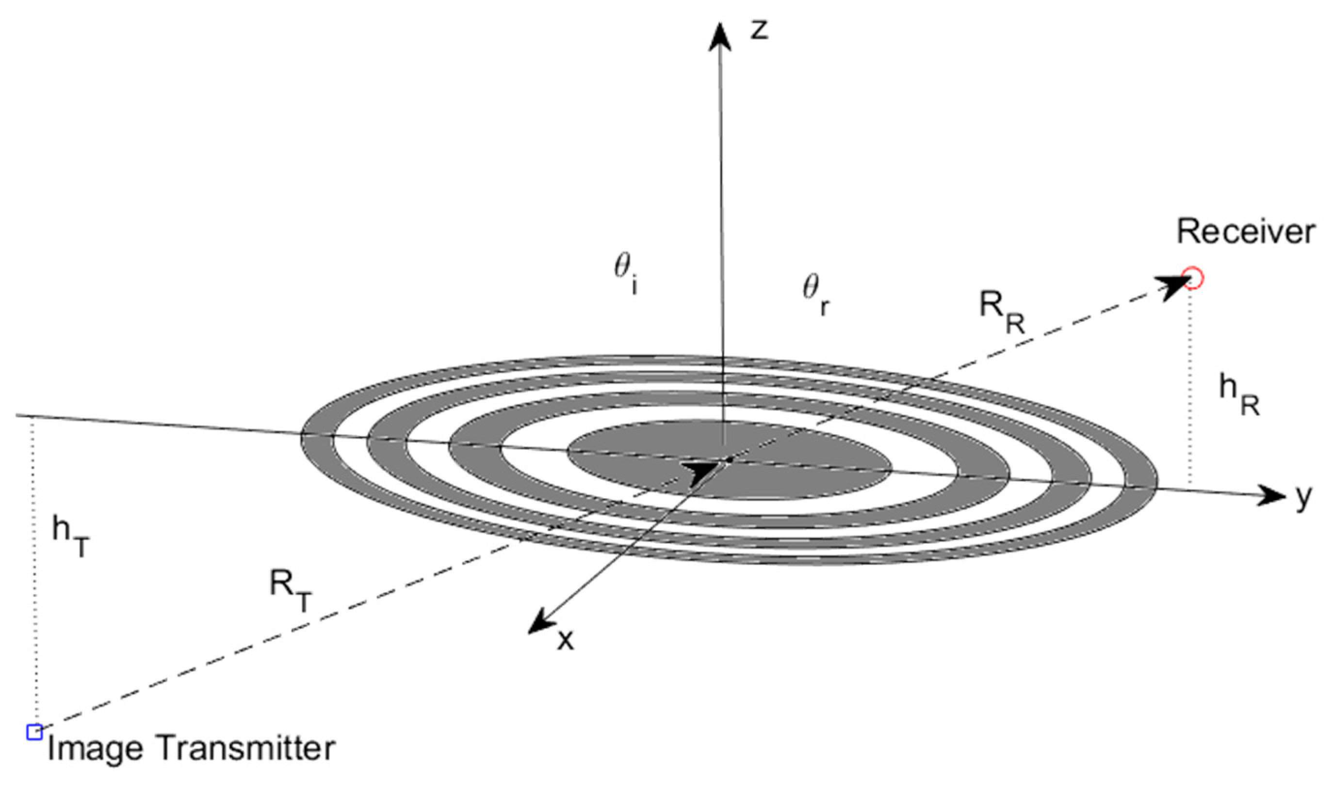
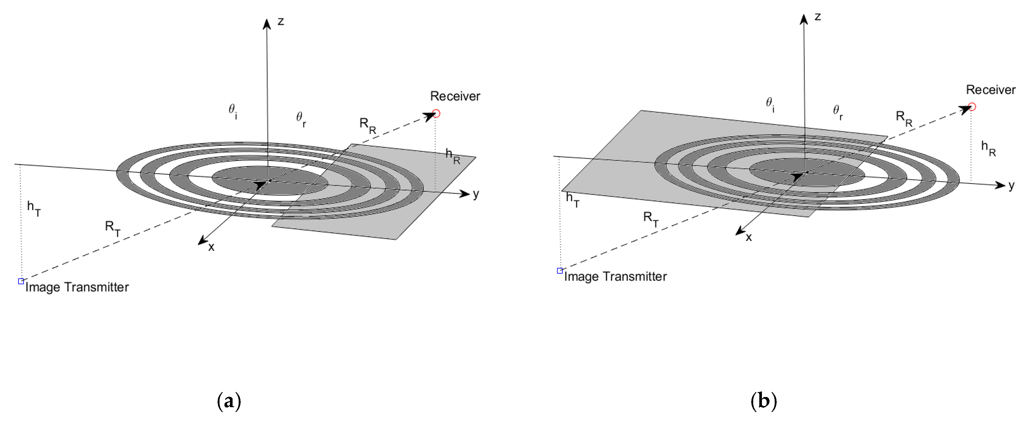
The scattering geometry is shown in Figure 1, where the receiver (R) and transmitter (T) lie in the YZ plane, and are at heights hR and hT over a flat surface. RT and RR are the distances to the origin of coordinates where the specular reflection point is, and θi is the incidence angle, which for the specular reflection point (origin of coordinates) is equal to the reflected angle θr. The different disks represent the Fresnel zones, with the odd ones (1, 3, 5, etc.) colored dark gray, and the even ones (2, 4, 6, etc.) colored white.
In what follows, a few principles of electromagnetism are reviewed. They will be used to compute a closed-form solution of the GNSS-R response to a step function, such as in the transition between water and the ocean.
2.1. Review of Some Basic Principles of Electromagnetism
2.1.1. Principle of Equivalence and Image Theory
The principle of equivalence [9] allows us to compute the solutions in the region of interest (half-space in front of the conducting plane) by replacing the plane conductor with the images of the dipoles. The image sources must satisfy the boundary condition that the tangential electric field at the conducting surface should be zero. The total electric field above the conducting plane (Figure 2) is then computed as the sum of the one created by the original currents and the image ones, while the total electric field below the conducting plane is zero. Applying this principle to our problem, the transmitter can be replaced by its “image” underneath the plane, as illustrated in Figure 3.
2.1.2. The Huygens Principle and Knife-Edge Diffraction
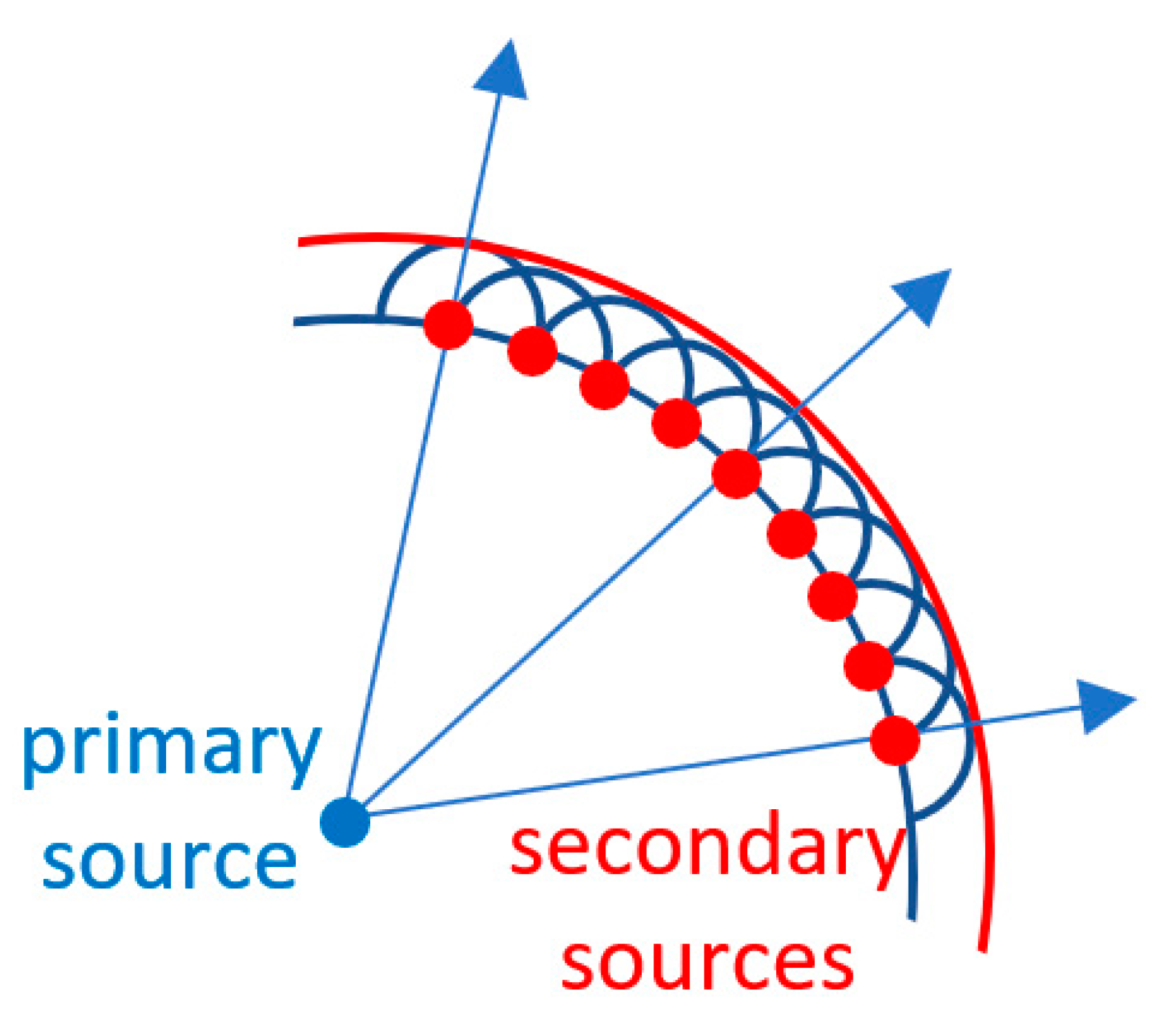
The Huygens principle states that every point (red dots in Figure 4) on a primary wave front (blue curve in Figure 4) may be regarded as a new source of spherical secondary waves, and that at each point in space these waves propagate in every direction at a speed and frequency equal to that of the primary wave, and in such a way that the primary wave front at some later time is the envelope of these secondary waves (red curve in Figure 4).
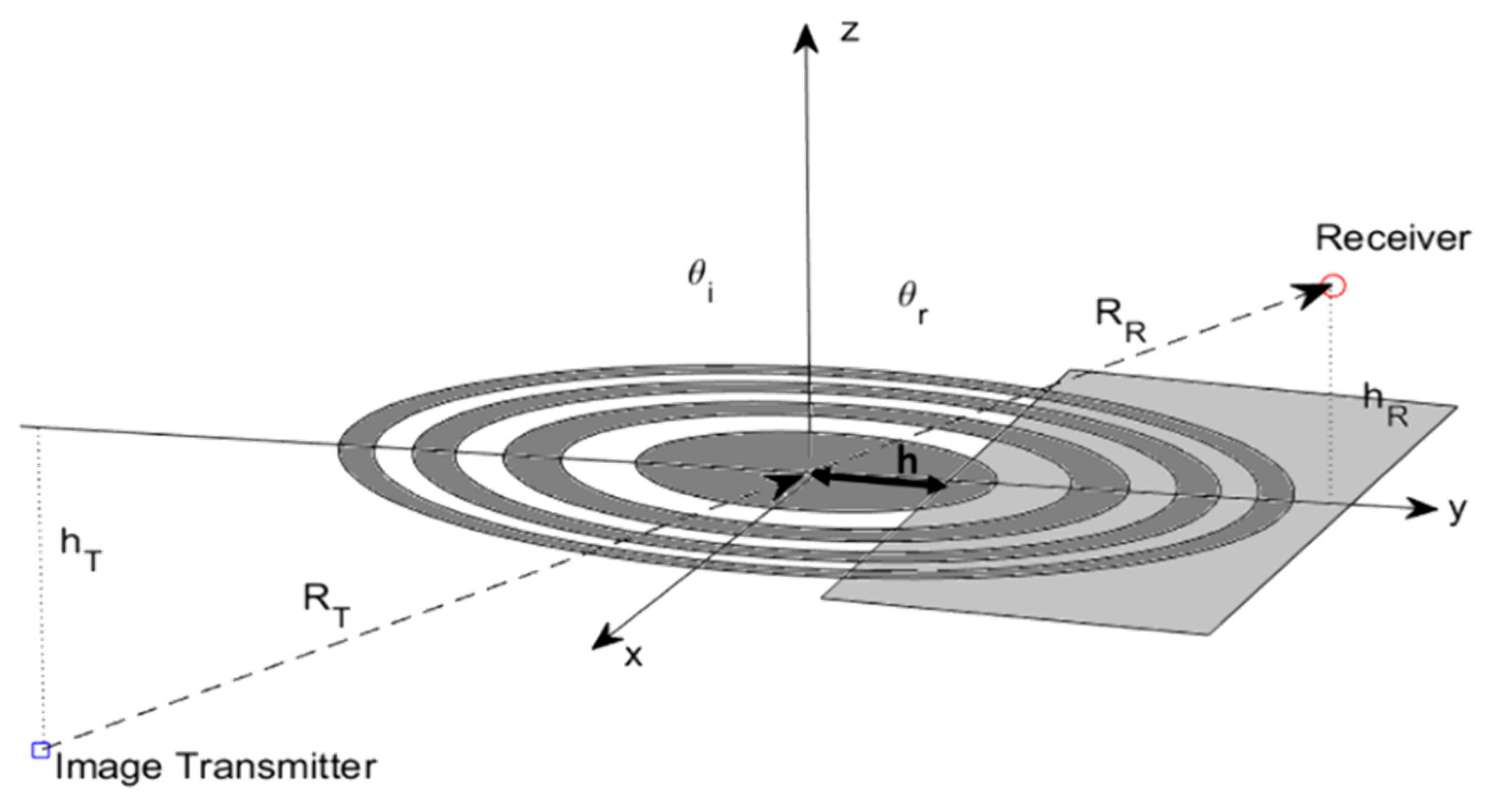
The Huygens principle can be applied to compute the electric fields when part of the trajectory is partially obstructed by a conducting plane as illustrated in Figure 5, leaving a clearance h with respect to the line of sight. This academic case is known as the “knife-edge diffraction”, and it is used in radio communications to assess the propagation losses with respect to the free space caused by the obstruction by a mountain, building, etc. In the latter this will represent the transition from one medium to another [6].
The development of an analytical solution can be found in many text books, and only the final result is provided below:
where:
and are the so-called Fresnel integrals, which are given be:
and is the Fresnel–Kirchhoff parameter:
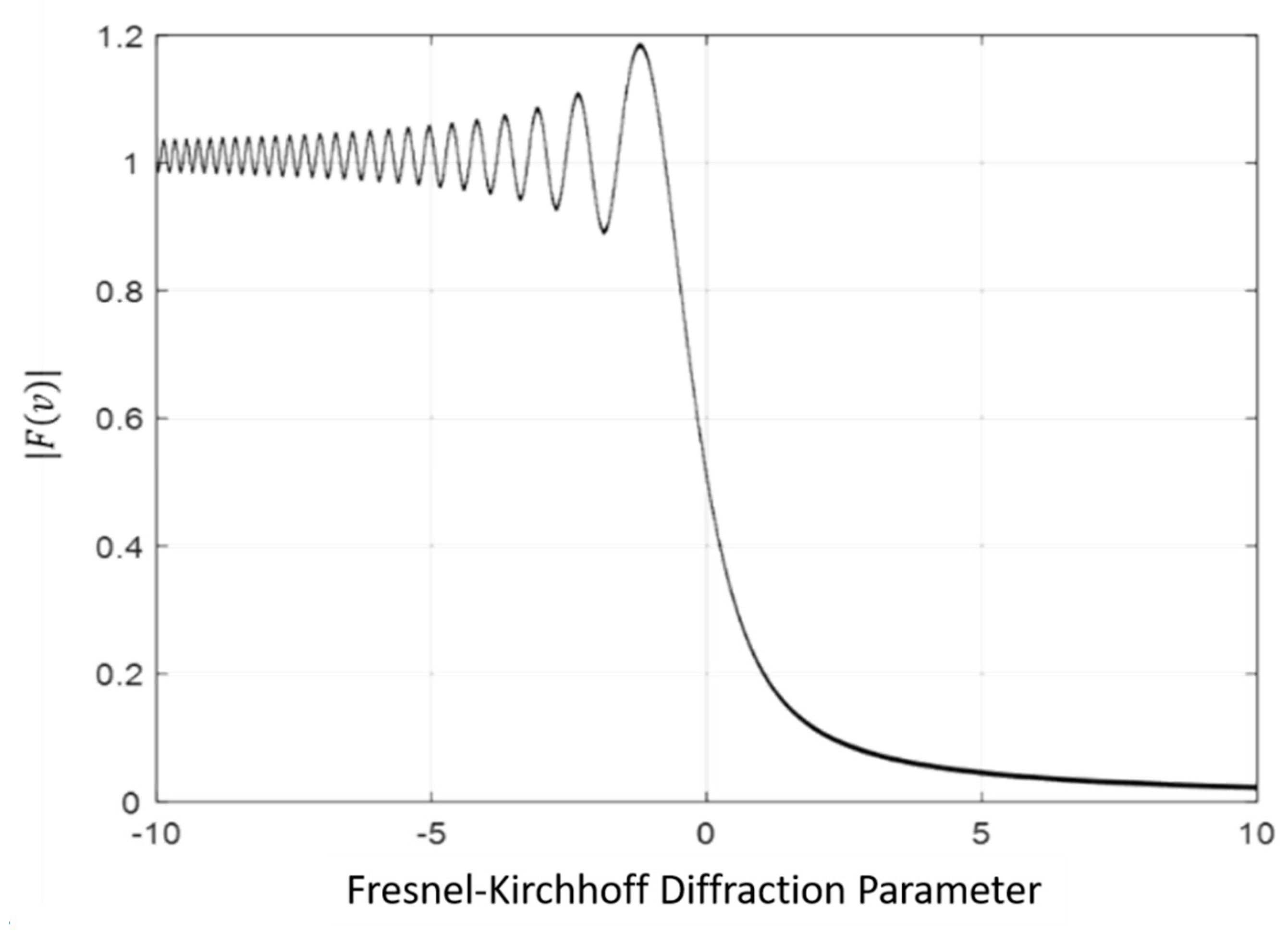
Figure 6 shows the absolute value of in Equation (3) in linear units. When h = 0, half of the electric field is blocked, which translates into a power loss of 6 dB with respect to the free-space conditions. Note the ringing for h < 0 due to the different Fresnel zones being blocked or not and contributing to the total electric field with different phases.
2.1.3. Babinet’s Principle
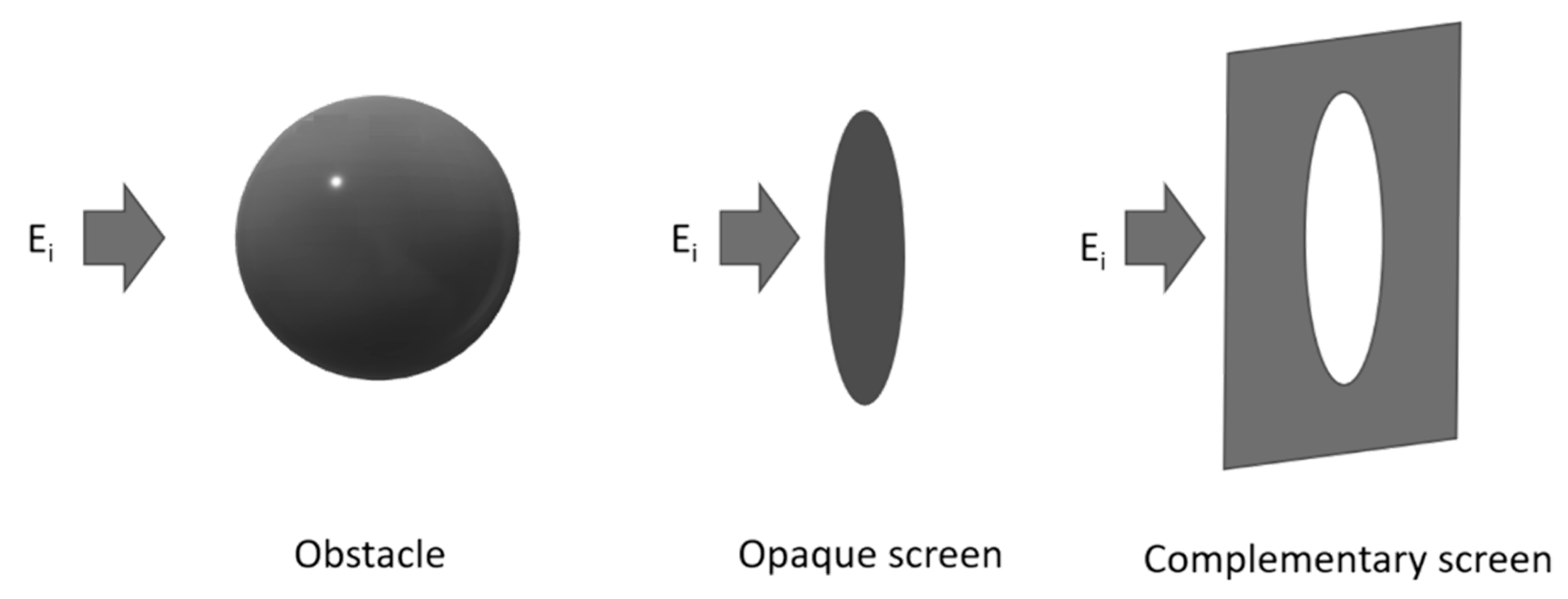
Babinet’s principle [10] states that the diffraction pattern from an opaque body is identical to that from a hole of the same size and shape, except for the overall forward beam intensity. The concept is expressed graphically in Figure 7 [11].
Babinet’s principle can be used to compute the electric field diffracted when the signal emitted by the transmitter’s image is diffracted by the light-gray opaque area in the z = 0 plane (the white area being “transparent”), and when it is diffracted by the white opaque area in the z = 0 plane (the light-gray area now being “transparent”).
2.1.4. Principle of Superposition
Once the electric fields diffracted by the semi-plane (the white area in the plane z = 0 in Figure 5) are computed, the electric fields diffracted by the complementary semi-plane (the light-gray area in the plane z = 0 in Figure 5), when it is not opaque, can be computed using Babinet’s principle, and then the total electric field arriving at the receiver can be computed as the sum of both.
2.2. Computation of the Electric Field Scattered by the Discontinuity between Two Media
Assuming that an electromagnetic wave impinges over the z = 0 plane around (x,y,z) = (0,0,0), where the specular reflection point is, and:
- The extension of the Fresnel reflection zones is small enough (a few hundred meters from a low Earth orbiter) so that the variations of the local incidence angle can be neglected over a few Fresnel zones;
- The plane z = 0 is composed of two flat half-planes of different materials, and thus exhibiting different reflection coefficients; and
- The transmission coefficient for the wave emitted by the image transmitter (Figure 5) is equal to the reflection coefficient evaluated at the local incidence angle at the origin.
Then, as illustrated in Figure 8, the total electric field can be immediately computed as the sum of the following two terms:
where is the Fresnel reflection coefficient, and is the dielectric constant of the half-plane n. The received power is proportional to the square of the absolute value of Equation (6).
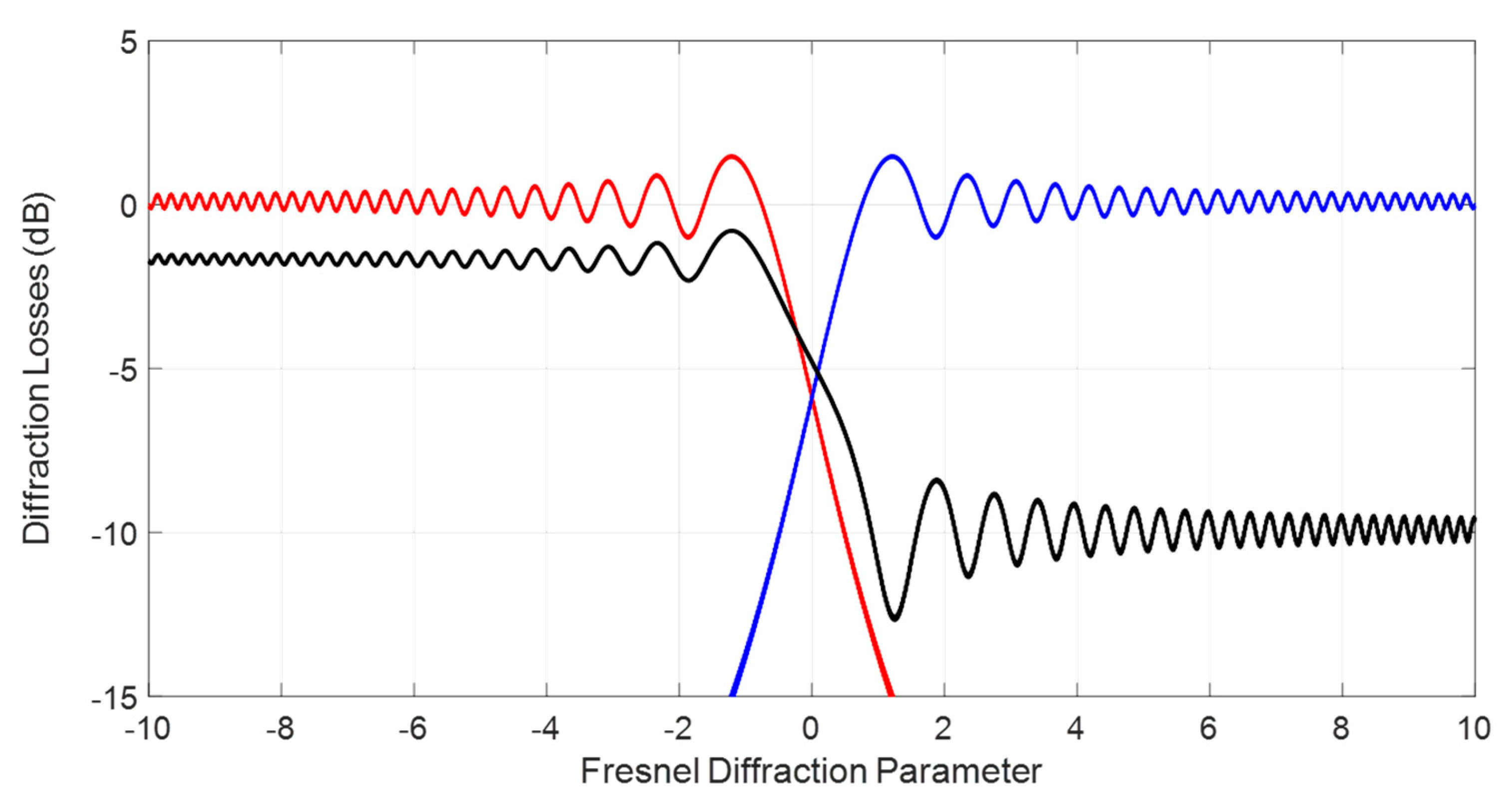
Following Equation (7), an example is shown in Figure 9. The red and blue lines correspond to and in decibels. The black line corresponds to the square of the absolute value of the term within brackets in Equation (7), computed for , and , which corresponds to the normalized peak power that would be collected by a GNSS-R instrument.
3. Results
3.1. Spatial Resolution Computation
Based on the above results the spatial resolution of a GNSS-R system can now be defined as the width of the transition from the 10% above , and 90% of
The solution of the above equations has to be performed numerically, and it actually depends on the values of and . The difference between and leads to the width of , , which is linked to the spatial resolution by means of Equation (9). For the sake of simplicity, assuming an airborne GNSS-R instrument, so that , and approximating , the following is an approximated formula for the spatial resolution:
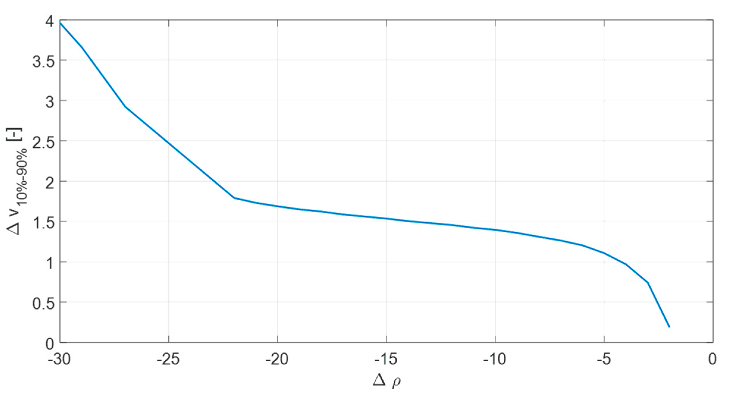
Figure 10 shows the evolution of as a function of in decibels. It varies from 0.74 for to 1.7 for This means that for a plane flying at hR = 1000 m height, at GPS L1/Galileo E1 (λ = 19 cm), the spatial resolution ranges from 7.2 m/cos(θi) to 16.6 m/cos(θi), depending on the contrast of the reflection coefficients in the transition.
3.2. Experimental Validation
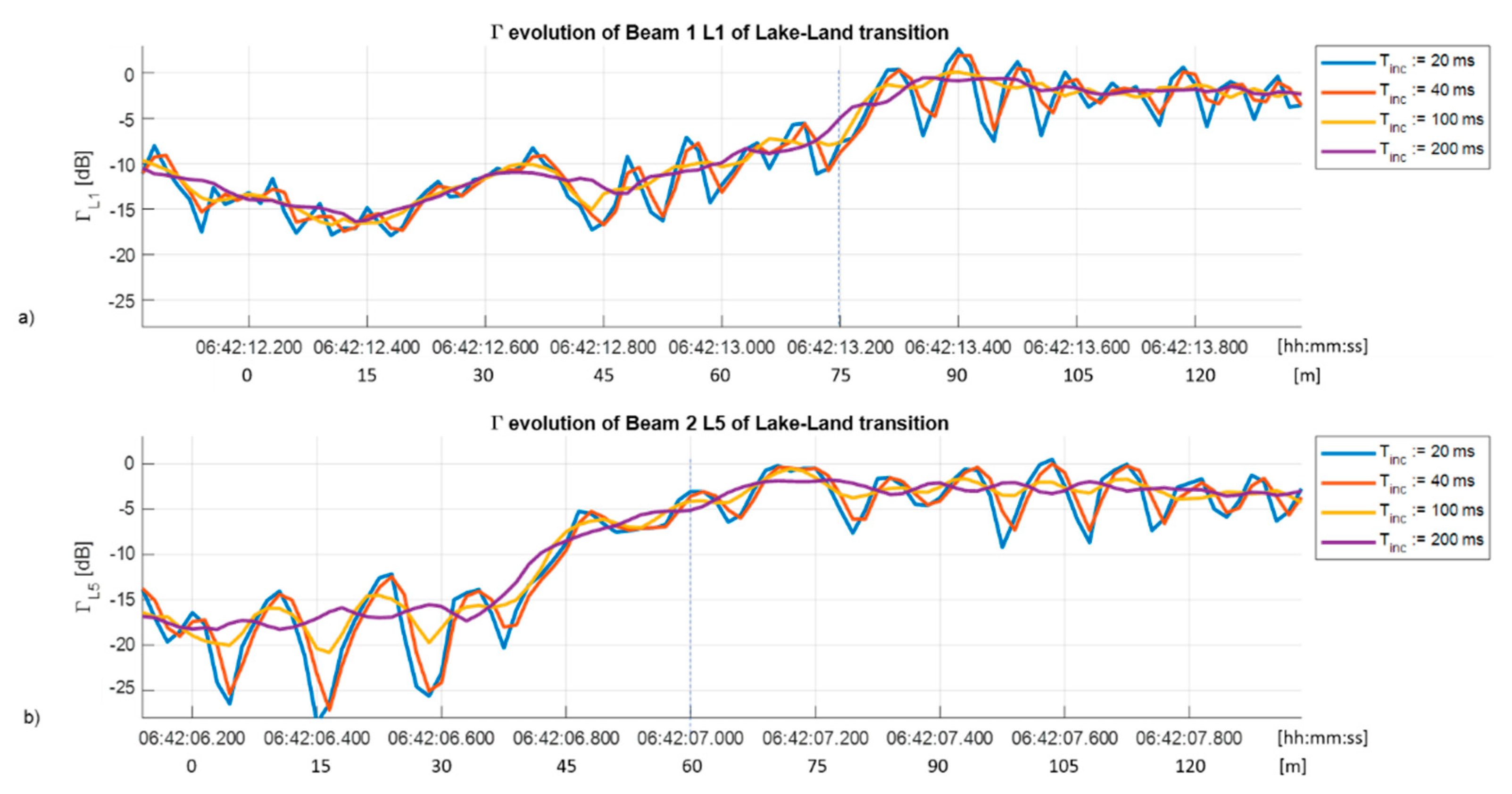
Figure 11 shows the measured reflectivity (Γ) in a transition between land and calm water in the Devilbend Reservoir, south of Melbourne, Victoria, Australia. The data was acquired during one of the test flights of the MIR [8] instrument on 30 April 2018. The top plot corresponds to one of the four beams at GPS L1, and the bottom plot at L5. Flight speed was 75 m/s, flight height was hR = 1000 m, and GNSS-R data were coherently integrated for 1 ms (GPS L1 C/A code), and incoherently for Tinc = 20, 40, 100, and 200 ms. At 20 ms, the blurring produced by the aircraft movement is 1.5 m, which is negligible compared to the best spatial resolution computed in Section 3.1. Inspecting Figure 11, at 20 and 40 ms incoherent integration time, one can clearly observe some reflectivity ripples that are reminiscent of those seen in Figure 9. At 100 ms, the blurring is 7.5 m, which is now comparable to the best spatial resolution, and the ripples can no longer be appreciated. At 200 ms the reflectivity plot is even smoother. In the land part (left part of the plots), note that the L5 reflections exhibit a more marked fading pattern than the L1 ones. This may be because L5 penetrates a bit more in the land (and vegetation), and it is moister soil underneath the surface. Although it is not very clear, the width of the reflectivity step is approximately 0.3 s, which corresponds roughly to 22.5 m, as compared to the 20.7 m predicted value using Equation (9) and Figure 10 for a ~−15 dB reflectivity.
Taking a closer look to the periodicity of the ripples, it can be observed that the period in Figure 11b is larger than that in Figure 11a, as it can be inferred from Equation (5), and Figure 6 and Figure 9, parameterized in terms of . In Figure 11a, the separation between consecutive peaks in time is ~100 ms, while in Figure 11b it is ~130 ms, which, for an aircraft speed of v = 75 m/s corresponds to 7.50 and 9.75 m, respectively. More detailed results are shown in Table 1 for several peaks. Replacing by in Equation (10), where being the angle formed between the aircraft ground-track and the coastline, one obtains:
Assuming hR = 1000 m, θi = 45°, and substituting for the time difference between consecutive peaks in Figure 11 (except for roundoff errors due to the discrete sampling), this ratio closely matches the squared root of the ratio of the wavelengths at L1 and L5: . Other sources of error are variations of the flight height (approximately hR = 1000 m), variations of the incidence angle, and most likely the fact that the velocity vector is not perpendicular to the coastline (as implicitly assumed in Figure 5).
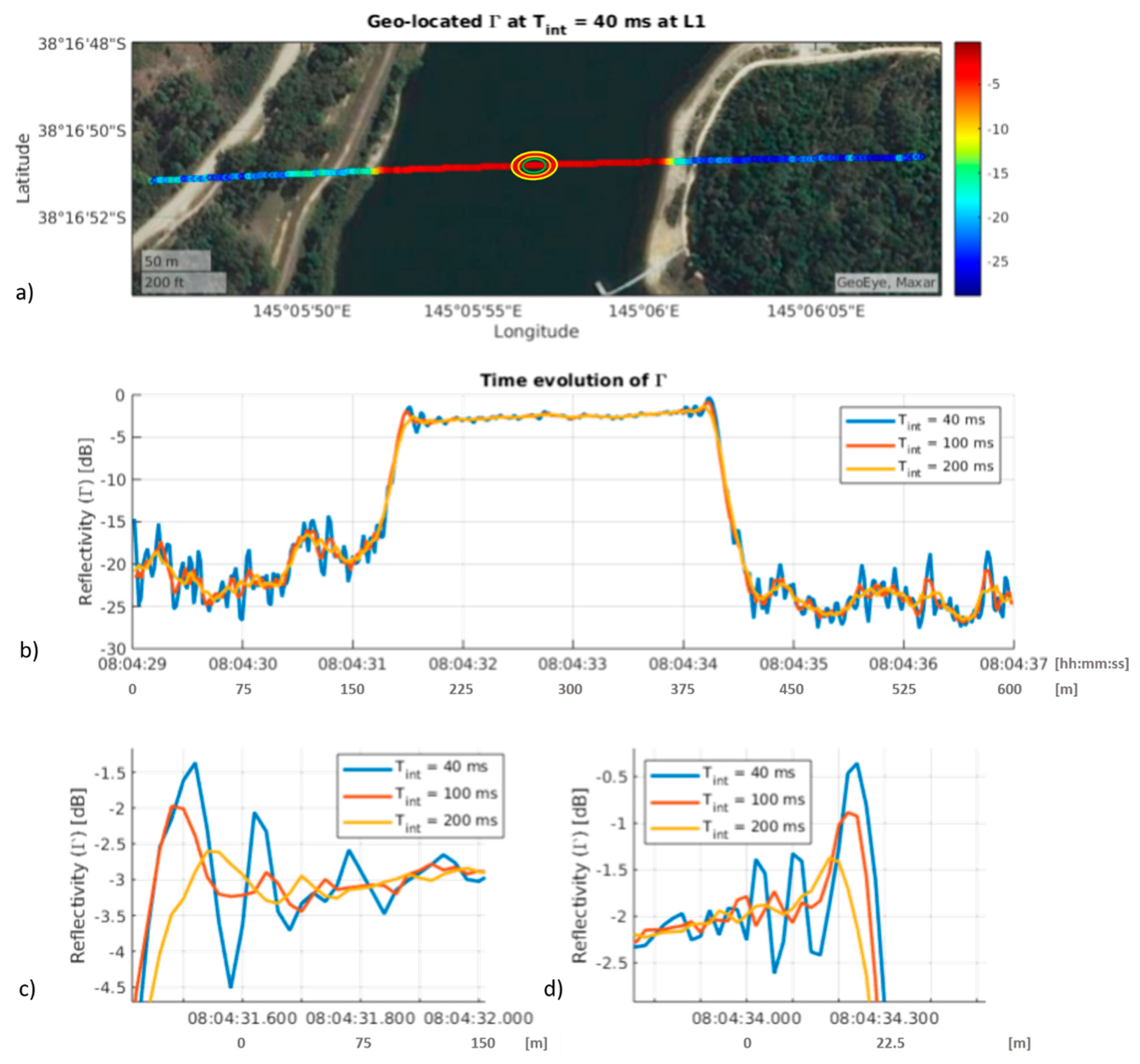
These results are corroborated by many other transitions. In what follows a few more examples are presented to illustrate this effect. A minimum incoherent integration time of 40 ms is used, since blurring is still negligible, and these results are almost identical to when 20 ms is used.
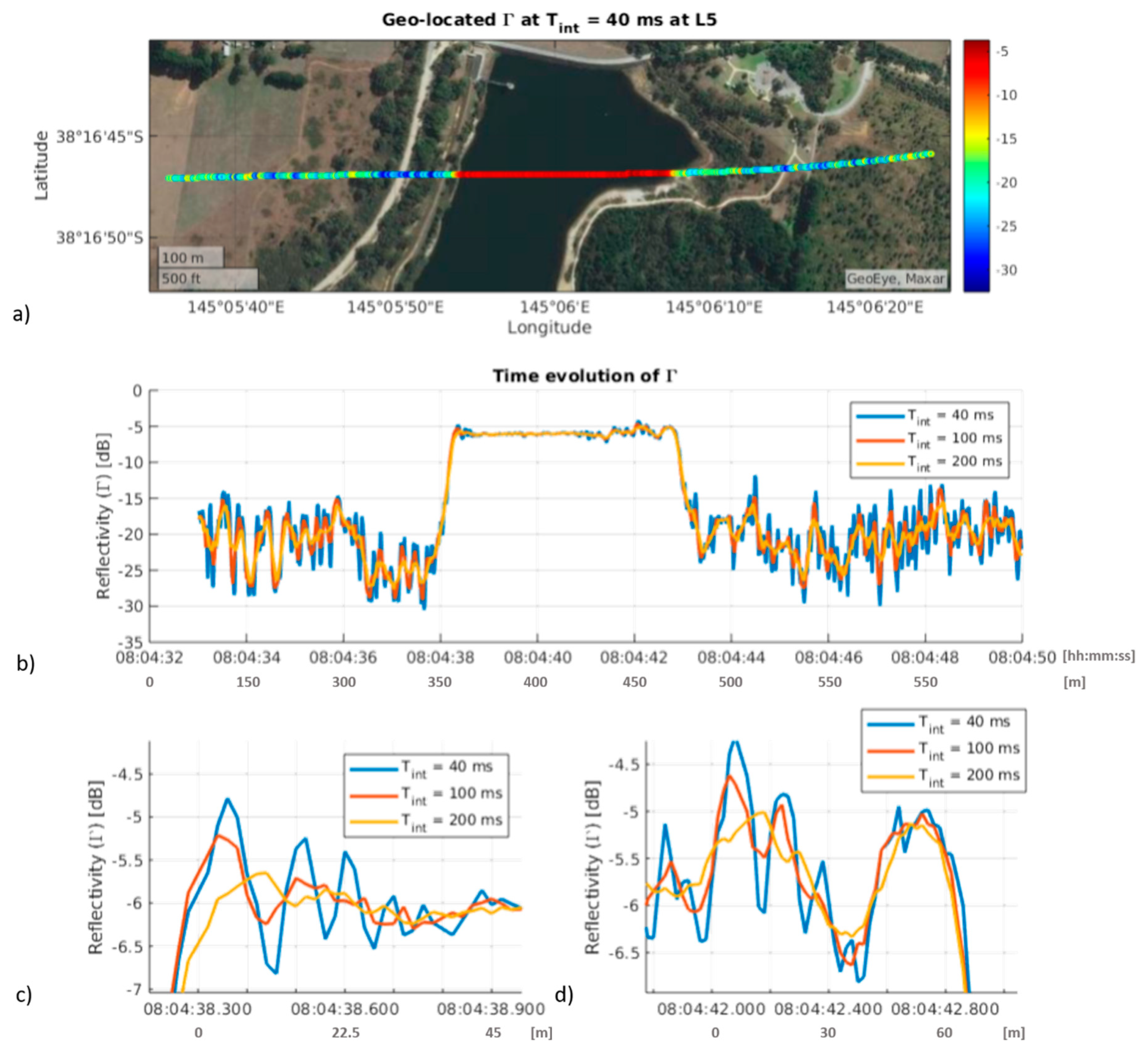
Figure 12 shows a geo-located double transition from land–calm water–land, the temporal evolution of the reflection coefficient at L1, and two zooms around the transitions for different incoherent integration times. Figure 13 shows another example at L5. Note that for large incoherent integration times (i.e., 200 ms) the ringings cannot be identified for both the L1 and L5 examples.
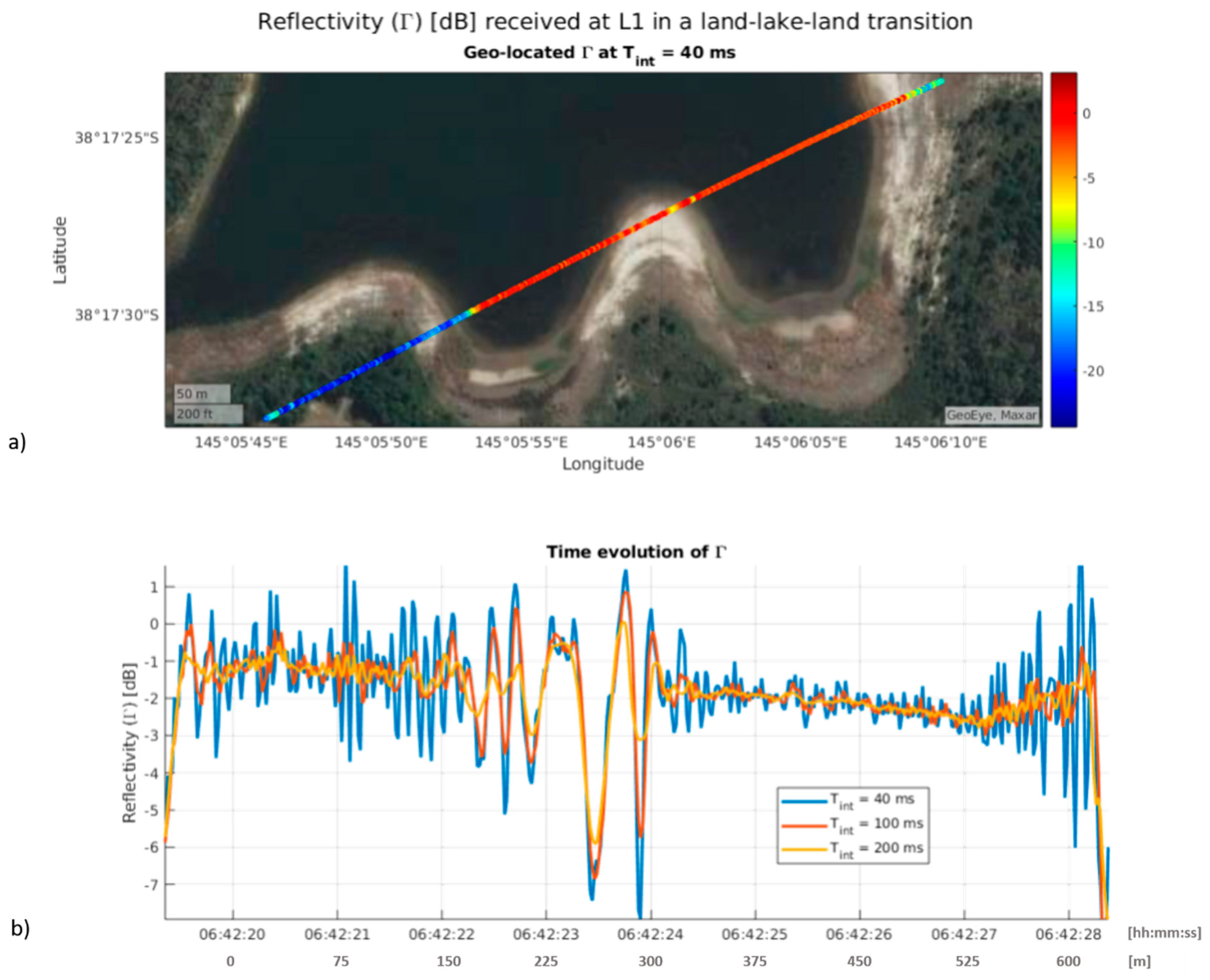
Figure 14 presents another example on the same flight. In this case, there is an additional transition to a small portion of a peninsula being crossed by the GNSS-R track. It can be noticed that at short integration times, some ripples are produced when changing from land to water, at the beginning and the end of the track. In addition, in the central part, when passing over the peninsula the combination of the different responses produces very large amplitude ripples. In this case, large incoherent integration times (i.e., 200 ms) are not blurring the ripples in the center of the image. However, if even larger integration times were used (i.e., 1 s) no ringings could be identified.
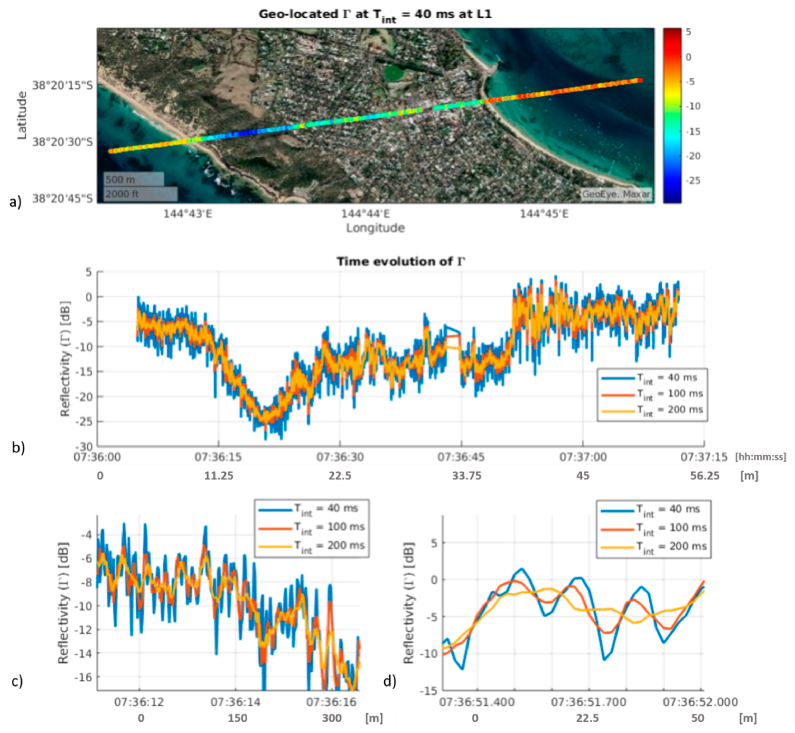
Finally, Figure 15 shows another double transition when passing over Sorrento, south of Melbourne. The left part corresponds to an open ocean area (Sorrento ocean beach), while the right part of the image is inside Port Phillip Bay (Sorrento front beach). Looking at the ocean–land transition in Figure 15c on the left-hand side, the reflectivity step is larger, but longer over time, and reflectivity values are noisy because of the increased surface roughness and speckle noise associated with a mostly incoherent scattering. The ripples described in the previous sections and illustrated in the previous examples can no longer be identified. However, as compared to the ocean side in Figure 15c, in Figure 15d the reflectivity step is smaller (calm water), but shorter in time (i.e., sharper), and similar ripples to the lake case can now be identified.
4. Discussion
To the authors’ best knowledge, this is the first analytical study of the response of a GNSS-R system to a reflectivity step. The analytical expression of the measured reflectivity can be derived from Equation (7):
with given by Equation (5). It shows a smooth transition between and , and ripples associated to different Fresnel zones passing from one area to the other one. The width of the transition, as measured from the 10% above the lowest reflectivity values to 90% of the highest reflectivity value, has been found to be dependent on the amplitude of the reflectivity step itself, although it is quite flat for a wide range of reflectivity steps (Figure 10):
The spatial resolution and the position of the peaks of the ripples was validated using airborne data at the L1 and L5 bands.
It is worth mentioning that the theoretical analysis assumes that coherent scattering is the dominant mechanism, which is the case when transitioning from land to/from calm water. However, when transitioning into open ocean, where incoherent scattering is more important, the presence of the ripples is not that evident, and the reflectivity exhibits random fluctuations associated mostly to the speckle noise.
These results should allow us to improve the determination of the extent of the flooded areas using GNSS-R observations as in [12,13,14,15], and they can also be used to dynamically optimize the coherent and incoherent integration times in future GNSS-R instruments (airborne or spaceborne) depending on the application or target area, as opposed to the approach implemented in past and current missions (1 ms coherent integration time, and 1 s incoherent integration time) such as UK TDS-1 [16] and NASA CyGNSS [17] missions.
5. Conclusions
In this study, the GNSS-R response to a step function in the reflectivity was derived analytically using known principles of electromagnetism. However, the evaluation of the Fresnel integrals has to be performed numerically. Analytical/numerical predictions match well with the experimental results at L1 and L5, acquired during an airborne experiment using the MIR (Microwave Interferometric Reflectometer) instrument over a water reservoir south of Melbourne and in a transition from the ocean into Port Phillip Bay, in terms of width and ringing, if incoherent integration times multiplied by the speed of the aircraft are shorter than the width of the Fresnel zone. Larger incoherent integration times blur the step response and degrade the achievable spatial resolution. Considering the size of the first Fresnel zone (tens of meters from a plane, to a few hundred meters from a spacecraft) the analysis presented is applicable to most coastlines.
Author Contributions
Conceptualization, A.C.; methodology, A.C.; software, J.F.M.-M. and A.C.; validation, A.C.; formal analysis, A.C.; investigation, A.C.; resources, A.C. and J.F.M.-M.; data curation, J.F.M.-M.; writing—original draft preparation, A.C.; writing—review and editing, A.C. and J.F.M.-M.; visualization, A.C. and J.F.M.-M.; supervision, A.C.; project administration, A.C.; funding acquisition, A.C. All authors have read and agreed to the published version of the manuscript.
Funding
This work was funded by the Spanish MCIU and EU ERDF project (RTI2018-099008-B-C21/AEI/10.13039/501100011033) “Sensing with pioneering opportunistic techniques” and grant to ”CommSensLab-UPC” Excellence Research Unit Maria de Maeztu (MINECO grant MDM-2016-600).
Acknowledgments
The authors would like to express their gratitude to R. Onrubia and D. Pascual who flew and operated the MIR instrument during the field experiment, and to C. Rüdiger, J.P. Walker, and A. Monerris for their support during the execution of the campaign.
Conflicts of Interest
The authors declare no conflict of interest.
References
- Zavorotny, V.U.; Gleason, S.; Cardellach, E.; Camps, A. Tutorial on Remote Sensing Using GNSS Bistatic Radar of Opportunity. IEEE Geosci. Remote Sens. Mag. 2014, 2, 8–45. [Google Scholar] [CrossRef] [Green Version]
- Martín-Neira, M. A passive reflectometry and interferometry system (PARIS): Application to ocean altimetry. ESA J. 1993, 17, 331–355. [Google Scholar]
- Clarizia, M.P.; Ruf, C.S. On the Spatial Resolution of GNSS Reflectometry. IEEE Geosci. Remote Sens. Lett. 2016, 13, 1064–1068. [Google Scholar] [CrossRef]
- Martin, F.; Camps, A.; Fabra, F.; Rius, A.; Martin-Neira, M.; D’Addio, S.; Alonso, A. Mitigation of Direct Signal Cross-Talk and Study of the Coherent Component in GNSS-R. IEEE Geosci. Remote Sens. Lett. 2015, 12, 279–283. [Google Scholar] [CrossRef]
- Munoz-Martin, J.F.; Onrubia, R.; Pascual, D.; Park, H.; Camps, A.; Rüdiger, C.; Walker, J.; Monerris, A. Untangling the Incoherent and Coherent Scattering Components in GNSS-R and Novel Applications. Remote Sens. 2020, 12, 1208. [Google Scholar] [CrossRef] [Green Version]
- Seybold, J.S. Introduction to RF Propagation, 8th ed.; John Wiley & Sons, Inc: Hoboken, NJ, USA, 2005. [Google Scholar] [CrossRef]
- Camps, A. Spatial Resolution in GNSS-R Under Coherent Scattering. IEEE Geosci. Remote Sens. Lett. 2020, 17, 32–36. [Google Scholar] [CrossRef]
- Onrubia, R.; Pascual, D.; Querol, J.; Park, H.; Camps, A. The Global Navigation Satellite Systems Reflectometry (GNSS-R) Microwave Interferometric Reflectometer: Hardware, Calibration, and Validation Experiments. Sensors 2019, 19, 1019. [Google Scholar] [CrossRef] [PubMed] [Green Version]
- Kong, J.A. Electromagnetic Wave Theory; EMW Publishing: Cambridge, MA, USA, 2008. [Google Scholar]
- Born, M.; Wolf, E. Principles of Optics; Cambridge University Press: Cambridge, UK, 1999. [Google Scholar]
- Kubicke, G.; Yahia, Y.A.; Bourlier, C.; Pinel, N.; Pouliguen, P. Bridging the Gap Between the Babinet Principle and the Physical Optics Approximation: Scalar Problem. IEEE Trans. Antennas Propag. 2011, 59, 4725–4732. [Google Scholar] [CrossRef]
- Nghiem, S.V.; Zuffada, C.; Shah, R.; Chew, C.; Lowe, S.T.; Mannucci, A.J.; Cardellach, E.; Brakenridge, G.R.; Geller, G.; Rosenqvist, A. Wetland monitoring with Global Navigation Satellite System reflectometry. Earth Space Sci. 2017, 4, 16–39. [Google Scholar] [CrossRef] [PubMed]
- Chew, C.; Reager, J.T.; Small, E. CYGNSS data map flood inundation during the 2017 Atlantic hurricane season. Sci. Rep. 2018, 8, 9336. [Google Scholar] [CrossRef] [PubMed]
- Loria, E.; O’Brien, A.; Zavorotny, V.; Downs, B.; Zuffada, C. Analysis of scattering characteristics from inland bodies of water observed by CYGNSS. Remote Sens. Environ. 2020, 245, 111825. [Google Scholar] [CrossRef]
- Unnithan, S.L.K.; Biswal, B.; Rüdiger, C. Flood Inundation Mapping by Combining GNSS-R Signals with Topographical Information. Remote Sens. 2020, 12, 3026. [Google Scholar] [CrossRef]
- Unwin, M.; Jales, P.; Tye, J.; Gommenginger, C.; Foti, G.; Rosello, J. Spaceborne GNSS-Reflectometry on TechDemoSat-1: Early Mission Operations and Exploitation. IEEE J. Sel. Top. Appl. Earth Obs. Remote Sens. 2016, 9, 4525–4539. [Google Scholar] [CrossRef]
- Ruf, C.S.; Chew, C.; Lang, T.; Morris, M.G.; Nave, K.; Ridley, A.; Balasubramaniam, R. A New Paradigm in Earth Environmental Monitoring with the CYGNSS Small Satellite Constellation. Sci. Rep. 2018, 8, 8782. [Google Scholar] [CrossRef] [PubMed] [Green Version]
Figure 1.
Global navigation satellite systems reflectometry (GNSS-R) scattering geometry showing the transmitter, receiver, specular reflection point (origin of coordinates), and the different Fresnel zones.
Figure 1.
Global navigation satellite systems reflectometry (GNSS-R) scattering geometry showing the transmitter, receiver, specular reflection point (origin of coordinates), and the different Fresnel zones.

Figure 2.
Left: linear and loop currents over a perfect conductor. Right: the conductor has been replaced by the image currents. Note that the sign reversal of the currents parallel to the conducting plane are responsible for the polarization change of the “reflected” wave.
Figure 2.
Left: linear and loop currents over a perfect conductor. Right: the conductor has been replaced by the image currents. Note that the sign reversal of the currents parallel to the conducting plane are responsible for the polarization change of the “reflected” wave.

Figure 3.
GNSS-R scattering geometry in Figure 1 modified according to the principle of equivalence: the transmitter is replaced by its image. Computed electric fields are only valid in the region z > 0.
Figure 3.
GNSS-R scattering geometry in Figure 1 modified according to the principle of equivalence: the transmitter is replaced by its image. Computed electric fields are only valid in the region z > 0.

Figure 4.
Graphical representation of the Huygens diffraction principle.

Figure 5.
Huygens principle applied to the “knife-edge diffraction” case. The light-gray area partially blocks the propagation of the signal, hiding parts of some Fresnel zones. h is the clearance of the obstruction.
Figure 5.
Huygens principle applied to the “knife-edge diffraction” case. The light-gray area partially blocks the propagation of the signal, hiding parts of some Fresnel zones. h is the clearance of the obstruction.

Figure 6.
Absolute value of . Negative indicates that the line-of-sight (LoS) trajectory is unobstructed, while positive indicates an LoS obstruction (see Figure 5).
Figure 6.
Absolute value of . Negative indicates that the line-of-sight (LoS) trajectory is unobstructed, while positive indicates an LoS obstruction (see Figure 5).

Figure 7.
Graphical representation of the concept of Babinet’s principle and the three equivalent obstacles: electric field incident on an arbitrary obstacle (left), associated opaque screen (center), and complementary screen (i.e., hole in the infinite plane; right).
Figure 7.
Graphical representation of the concept of Babinet’s principle and the three equivalent obstacles: electric field incident on an arbitrary obstacle (left), associated opaque screen (center), and complementary screen (i.e., hole in the infinite plane; right).

Figure 8.
Graphical representation of the principle of superposition and its application to the computation of the total electric field incident. Opaque screen on the (a) right and (b) left sides block radiation.
Figure 8.
Graphical representation of the principle of superposition and its application to the computation of the total electric field incident. Opaque screen on the (a) right and (b) left sides block radiation.

Figure 9.
Graphical representation of the (red) and (blue) functions, and total power loss computed as (black) for and .
Figure 9.
Graphical representation of the (red) and (blue) functions, and total power loss computed as (black) for and .

Figure 10.
Width of the parameter for a transition from 10% above to 90% of .

Figure 11.
Land-to-water transition during a Microwave Interferometric Reflectometer (MIR) test flight over Devilbend Reservoir (38.29°S, 145.1°E): (a) GPS L1, (b) GPS L5. Horizontal axis units: time and distance. Vertical dashed line: land–water transition.
Figure 11.
Land-to-water transition during a Microwave Interferometric Reflectometer (MIR) test flight over Devilbend Reservoir (38.29°S, 145.1°E): (a) GPS L1, (b) GPS L5. Horizontal axis units: time and distance. Vertical dashed line: land–water transition.

Figure 12.
Land-to-water transition during an MIR at L1 test flight over Devilbend Reservoir (38.29°S, 145.1°E). (a) Geo-located reflectivity, and approximated representation of the first four Fresnel zones; (b) time evolution of the reflectivity, and a zoom-in of the step transition on the (c) left and (d) right.

Figure 13.
Land-to-water transition during a MIR at L5 test flight over Devilbend Reservoir (38.29°S, 145.1°E). (a) Geo-located reflectivity, (b) time evolution of the reflectivity, and a zoom-in of the step transition on the (c) left and (d) right.
Figure 13.
Land-to-water transition during a MIR at L5 test flight over Devilbend Reservoir (38.29°S, 145.1°E). (a) Geo-located reflectivity, (b) time evolution of the reflectivity, and a zoom-in of the step transition on the (c) left and (d) right.

Figure 14.
Land-to-water transition during an MIR at L1 test flight over Devilbend Reservoir (38.29°S, 145.1°E). (a) Geo-located reflectivity, and (b) time evolution of the reflectivity.
Figure 14.
Land-to-water transition during an MIR at L1 test flight over Devilbend Reservoir (38.29°S, 145.1°E). (a) Geo-located reflectivity, and (b) time evolution of the reflectivity.

Figure 15.
Land-to-water transition during an MIR at L1 test flight over Point Nepan, Melbourne (38.35°S, 144.74°E). (a) Geo-located reflectivity, (b) time evolution of the reflectivity, and a zoom-in of the step transition on the (c) left and (d) right.
Figure 15.
Land-to-water transition during an MIR at L1 test flight over Point Nepan, Melbourne (38.35°S, 144.74°E). (a) Geo-located reflectivity, (b) time evolution of the reflectivity, and a zoom-in of the step transition on the (c) left and (d) right.


Table 1.
Peak positions in Figure 6 and peak spacing ( ), peak positions in time for L1 and L5 beams, time spacing and estimated peak spacing in .
Table 1.
Peak positions in Figure 6 and peak spacing ( ), peak positions in time for L1 and L5 beams, time spacing and estimated peak spacing in .
[s] | [ms] | [s] | [ms] | ||||
|---|---|---|---|---|---|---|---|
| −1.22 | - | Not visible | - | - | 7.140 | - | |
| −2.34 | 1.12 | 13.290 | - | - | 7.310 | 170 | 0.95 |
| −3.08 | 0.74 | 13.400 | 110 | 0.71 | 7.450 | 140 | 0.67 |
| −3.68 | 0.60 | 13.500 | 100 | 0.65 | 7.570 | 120 | 0.78 |
| −4.18 | 0.50 | 13.580 | 80 | 0.52 | 7.700 | 130 | 0.67 |
Publisher’s Note: MDPI stays neutral with regard to jurisdictional claims in published maps and institutional affiliations. |
© 2020 by the authors. Licensee MDPI, Basel, Switzerland. This article is an open access article distributed under the terms and conditions of the Creative Commons Attribution (CC BY) license (http://creativecommons.org/licenses/by/4.0/).
Share and Cite
MDPI and ACS Style
Camps, A.; Munoz-Martin, J.F. Analytical Computation of the Spatial Resolution in GNSS-R and Experimental Validation at L1 and L5. Remote Sens. 2020, 12, 3910. https://0-doi-org.brum.beds.ac.uk/10.3390/rs12233910
AMA Style
Camps A, Munoz-Martin JF. Analytical Computation of the Spatial Resolution in GNSS-R and Experimental Validation at L1 and L5. Remote Sensing. 2020; 12(23):3910. https://0-doi-org.brum.beds.ac.uk/10.3390/rs12233910
Chicago/Turabian StyleCamps, Adriano, and Joan Francesc Munoz-Martin. 2020. "Analytical Computation of the Spatial Resolution in GNSS-R and Experimental Validation at L1 and L5" Remote Sensing 12, no. 23: 3910. https://0-doi-org.brum.beds.ac.uk/10.3390/rs12233910
Note that from the first issue of 2016, this journal uses article numbers instead of page numbers. See further details here.