Article

Development of an Improved Model for Prediction of Short-Term Heavy Precipitation Based on GNSS-Derived PWV

1
School of Environment Science and Spatial Informatics, China University of Mining and Technology, No.1 Daxue Road, Xuzhou 221116, China
2
Aerospace Information Research Institute, Chinese Academy of Sciences, No.9 Dengzhuang South Road, Haidian District, Beijing 100094, China
3
Satellite Positioning for Atmosphere, Climate and Environment (SPACE) Research Center, RMIT University, Melbourne, VIC 3001, Australia
4
School of Land Science and Technology, China University of Geosciences (Beijing), 29 Xueyuan Road, Haidian District, Beijing 100083, China
5
Research Center of Beidou Navigation and Remote Sensing, Suzhou University of Science and Technology, Suzhou 215009, China
*
Author to whom correspondence should be addressed.
Remote Sens. 2020, 12(24), 4101; https://0-doi-org.brum.beds.ac.uk/10.3390/rs12244101
Submission received: 18 November 2020 / Revised: 11 December 2020 / Accepted: 12 December 2020 / Published: 15 December 2020
(This article belongs to the Special Issue Climate Modelling and Monitoring Using GNSS)

Abstract

:
Nowadays, the Global Navigation Satellite Systems (GNSS) have become an effective atmospheric observing technique to remotely sense precipitable water vapor (PWV) mainly due to their high spatiotemporal resolutions. In this study, from an investigation for the relationship between GNSS-derived PWV (GNSS-PWV) and heavy precipitation, it was found that from several hours before heavy precipitation, PWV was probably to start with a noticeable increase followed by a steep drop. Based on this finding, a new model including five predictors for heavy precipitation prediction is proposed. Compared with the existing 3-factor model that uses three predictors derived from the ascending trend of PWV time series (i.e., PWV value, PWV increment and rate of the PWV increment), the new model also includes two new predictors derived from the descending trend: PWV decrement and rate of PWV decrement. The use of the two new predictors for reducing the number of misdiagnosis predictions is proposed for the first time. The optimal set of monthly thresholds for the new five-predictor model in each summer month were determined based on hourly GNSS-PWV time series and precipitation records at three co-located GNSS/weather stations during the 8-year period 2010–2017 in the Hong Kong region. The new model was tested using hourly GNSS-PWV and precipitation records obtained at the above three co-located stations during the summer months in 2018 and 2019. Results showed that 189 of the 198 heavy precipitation events were correctly predicted with a lead time of 5.15 h, and the probability of detection reached 95.5%. Compared with the 3-factor method, the new model reduced the FAR score by 32.9%. The improvements made by the new model have great significance for early detection and predictions of heavy precipitation in near real-time.

Graphical Abstract

1. Introduction

Precipitation is one of the most pivotal processes of the hydrologic cycle on the earth. However, heavy precipitation greatly affects the natural environment and the sustainability of our human society, which often brings serious environmental deterioration and enormous economic losses. Thus, the monitoring and prediction of precipitation has attracted much attention in the past decade, especially for highly populated and highly moist metropolises such as Hong Kong [1,2]. As a type of meteorological data, atmospheric water vapor is generally expressed in precipitable water vapor (PWV) and defined as the total atmospheric water vapor contained in a vertical column of unit area. Since the occurrence of severe weather events such as typhoons, thunderstorms and heavy precipitation strongly correlates with large temporal variations in PWV [3,4,5,6], PWV time series with high accuracy and resolutions are often used in the predictions for precipitation and other severe weather events [7,8]. Traditional technologies for measuring water vapor, e.g., radiosonde [9], water vapor radiometer [10] and satellite-based instruments [11], have been widely applied in meteorology [12,13]. Although the accuracy of water vapor obtained from these technologies is generally high, these technologies have some limitations, e.g., one-off attribute, high operational cost, low spatiotemporal resolution and limited to some weather conditions [14,15,16]. Consequently, these technologies can hardly satisfy some meteorological applications, especially for short-term weather monitoring and predictions [17,18]. This is the main motivation to use a new means, Global Navigation Satellite Systems (GNSS), to remotely sense the atmospheric water vapor content [19,20,21,22,23,24], due to its 24-h variability, high accuracy, global coverage, low cost, long-term stability, high spatiotemporal resolution and all-weather operability [25,26,27,28,29]. PWV over a ground-based GNSS station can be obtained from a conversion of the tropospheric delay estimated from the GNSS signal observed at the station, and this PWV is often called GNSS-PWV. Nowadays, many regional and global GNSS networks, which consist of various numbers of tracking stations, are available. This makes the best use of GNSS data for studies and applications on short-term weather predictions feasible and meaningful [17,30,31,32], in addition to facilitating climate change research [33,34,35].
As previous studies revealed, a precipitation event highly correlates with the intensity of regional PWV variation [36,37,38]. Singh et al. [39] analyzed monthly and seasonal PWV variations over the Arabian Sea and the Bay of Bengal and found a close relationship between PWV variation and monsoon; then Singh et al. [40] claimed that PWV can be used as an indicator in monsoon forecasting. Champollion et al. [41] stated that heavy precipitation events are associated with ongoing accumulation of water vapor, based on a case study of torrential precipitation in France. Van Baelen et al. [8] investigated the variations in GNSS-PWV in the duration of precipitation life cycles and concluded that water vapor plays a dominant role in the evolution of precipitation events. Chen et al. [2] also demonstrated that water vapor data with a high accuracy and high spatio-temporal resolution are useful for determining the onset of heavy precipitation events. According to the proved positive relationship between the intensity of regional PWV variation and the occurrence of precipitation events, several researchers conducted investigations on the use of GNSS-PWV in the monitoring and prediction of precipitation. Based on the fact that when the PWV values over a certain period of time are above a certain threshold, the probability of precipitation occurrence would greatly increase. Kedem et al. [42] proposed a threshold-based precipitation prediction model, which has also been validated in several studies [43,44]. For example, Shoji et al. [45] verified that the phenomenon of PWV reaching a defined threshold is an effective indication of a convective precipitation event. Shi et al. [46] presented some precipitation cases with different strengths happened in the city of Wuhan, China, to indicate the feasibility of using an empirical GNSS-PWV threshold for precipitation prediction. Yeh et al. [47] also determined GNSS-PWV threshold values for various precipitation strengths in Taiwan over the period 2006–2012. Although this type of approach is easy and may be effective in some cases, its prediction results are likely to be unstable and have low accuracy. Using the GNSS-PWV value as the sole criterion of precipitation prediction is deficient as it can only reflect the one-dimensional (zenith) distribution of water vapor and is likely to result in high false alarm rates [48,49,50]. The rapid developments of the GNSS tropospheric tomography in the past two decades have also made the use of this maturing technique to obtain high accuracy three-dimensional water vapor profile, which has already been used in applications of GNSS meteorology [51,52,53]. Therefore, some researchers proposed that, in addition to the threshold for GNSS-PWV, a long GNSS-PWV time series [54,55], a high temporal resolution dataset [56,57], multidimensional GNSS tomography-based water vapor profiles [58,59] and numerous other predictors obtained from GNSS observations can be used for precipitation prediction [60,61,62,63]. Among them, Benevides et al. [48] analyzed the characteristics of the temporal variation in PWV during the period of 2010–2012 in Lisbon for heavy precipitation in several case studies and proposed a simple model for predicting precipitation within 6 h. The maximum rate of PWV increment was also used as a predictor in the model, and the test results of the model showed a 75% correct detection rate and a false alarm rate of 65%. Based on the above researches, Yao et al. [49] proposed a 3-factor prediction method, and the three factors are PWV value, PWV variation and the rate of PWV variation. The method further improved the correct detection rate of precipitation prediction to 82%, while the false alarm rate was 66%, which was slightly worse. Zhao et al. [57] employed the PWV increment and PWV slope during the PWV ascending period prior to precipitation, and its prediction result showed that above 90% of heavy precipitation were successfully predicted, while the false alarm rate was 60%–70%, which is relatively high. Manandhar et al. [55] used data from a tropical region and proposed an algorithm for two predictors, the maximum PWV value (major predictor) and the rate of PWV increment, and this algorithm reduced the false alarm rate by 17%. Moreover, an improved rainfall forecasting model (IRFM) was also proposed by Zhao et al. [50] to predict rainfall based on five predictors including monthly PWV, seasonal PWV/ZTD variations and their first derivatives, and results showed the mean correct detection rate was better than 95% and the false alarm rate was less than 30%.
In all the aforementioned methods, the predictors are all obtained from the ascending trend in the GNSS-PWV time series. In fact, due to the diffusional and collisional growth of cloud droplets and raindrops, a sharp drop in the GNSS-PWV time series also occurs during the evolution of heavy precipitation [64,65]. This phenomenon has been confirmed by several researchers, e.g., Madhulatha et al. [66] reported that a noticeable decrease in GNSS-PWV was found 3 h prior to a storm development. Barindelli et al. [67] also found a steep decrease of 5–10 mm/h in the PWV time series in response to a heavy precipitation event. Zhang et al. [68] stated that a sharp drop in PWV coincides with the passing of extreme precipitation. Jones et al. [38] claimed that during the warm convective season a thunderstorm happened 3.5 h after the PWV reached the peak. These results imply that the phenomenon of a sharp decrease in PWV during the evolution of heavy precipitation may be also used as a possible predictor for heavy precipitation detection. Therefore, this study proposes a new model that includes not only the commonly used three predictors from the ascending trend, but also two additional predictors from the descending trend of GNSS-PWV time series for short-term prediction of heavy precipitation.
The structure of the paper is outlined as follows. Section 2 gives a description of data and methodologies adopted in this study. The relationship between GNSS-PWV and precipitation is analyzed and presented in Section 3, followed by Section 4 for the development and validation of the new model proposed in this study. Discussions and conclusions are given in Section 5 and Section 6, respectively.

2. Data and Methodologies

2.1. Selection of Data

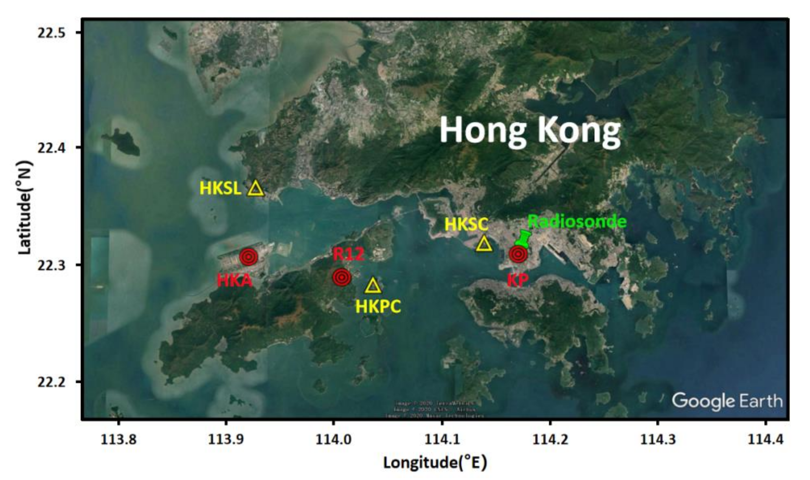
2.1.1. Selection of Location and Data Period

Hong Kong, located at the coast of South China Sea (SCS), has a humid subtropical climate greatly influenced by the Asian Summer Monsoon (ASM) [2,69]. Identified as one of the main low-level monsoonal streams, the ASM from the SCS transports huge amounts of water vapor towards Hong Kong during its occurrence [70,71]. During the summer months, Hong Kong often experiences severe weather events like hail, thunderstorms, typhoons and increased heavy precipitation events [72]. According to the criteria for precipitation intensity defined by World Meteorological Organization (WMO), a heavy precipitation event is regarded as precipitation if hourly precipitation falls in the range from 10 mm to 50 mm or daily precipitation is above 50 mm [73,74]. Based on this definition, over 56% heavy precipitation occurred in summer months (June, July and August in the northern hemisphere), as recorded at the Hong Kong Observatory (HKO) from 1885 to 2019 (excluding 1940–1946) [75]. Thus, this study mainly focused on heavy precipitation events happened in each summer month in the Hong Kong region.

2.1.2. Selection of Experimental Data

To analyze the relationship between GNSS-PWV and precipitation and improve the performance of prediction for heavy precipitation events, the data used in this study, mainly including GNSS-PWV time series from some local GNSS tracking/reference stations and heavy precipitation records from the weather stations that are close to the GNSS stations, i.e., the so-called co-located stations. The selection of GNSS stations for testing is merely based on the availability of both GNSS observations and precipitation records at co-locations during the summer months over the 10-year period from 2010 to 2019. It is noted that, if the distance between a GNSS station and a weather station is within a certain value, e.g., a few kilometers, then the two stations are regarded co-located. In the Hong Kong region, only three GNSS tracking stations, HKSC, HKSL and HKPC, satisfy the above conditions. The location of the three GNSS stations and their co-located weather stations (KP, HKA, and R12) are listed in Table 1 and Figure 1 illustrates their geographical distribution. The distances of all the three pairs of co-located stations are all under 3.3 km. In addition, Figure 1 also shows the only radiosonde station deployed in Hong Kong as the radiosonde data from this station were also used to evaluate the accuracy of GNSS-PWV.

2.2. GNSS Data

2.2.1. Retrieval of GNSS-PWV

The GNSS signal received by a ground-based GNSS receiver is delayed by the atmosphere when it transmits from the satellite to the receiver, and the atmospheric delay consists of the tropospheric delay and ionospheric delay. The tropospheric delay, together with other geodetic parameters, can be estimated from the GNSS observations [21,22,76]. In this study, the tropospheric zenith total delay (ZTD) during the 10-year period 2010–2019 at the three selected GNSS stations (shown in Figure 1 and Table 1) was estimated from the GNSS data using Bernese V5.2 [77] with the Vienna Mapping Function 1 (VMF1) [78] and the elevation cut-off angle of 3°. Then, the commonly used Saastamoinen model was used to obtain the zenith hydrostatic delay (ZHD) [79], which is a function of surface pressure measured [20]:
Z H D = 2.2779 ± 0.0024 P 0 f φ ,   H
where P0 is the pressure (hPa) at the height of the site; f φ , H is a function for the gravitational acceleration, which can be expressed as:
f φ , H = 1 0.00266 × cos 2 φ 0.00028 H
where φ and H are the latitude (°) and height (km) above the reference ellipsoid of the site, respectively.
The zenith wet delay (ZWD) over the GNSS station is then obtained from subtracting the ZHD from the ZTD, then the ZWD is converted to GNSS-PWV (mm) using the following formula [32]:
P W V = Π × Z W D
where Π is the conversion factor and can be obtained by
Π = 10 6 ρ w a t e r R w k 3 T m + k 2
k 2 = k 2 k 1 R d R w
where ρ w a t e r is the density of liquid water; R w and R d are the specific gas constants for WV and dry air, respectively; k1, k2 and k3 are three physical constants, which can be obtained from the commonly used formula for atmospheric refractivity, as suggested by Bevis et al. [33]; T m is the weighted mean temperature along the vertical direction over the station. In this study, the linear model developed by Chen [80] based on 8-year meteorological data in Hong Kong was used to obtain T m for the station:
T m = 106.7 + 0.605 T s + 273.15
where T s is the surface temperature (°C) of the station.

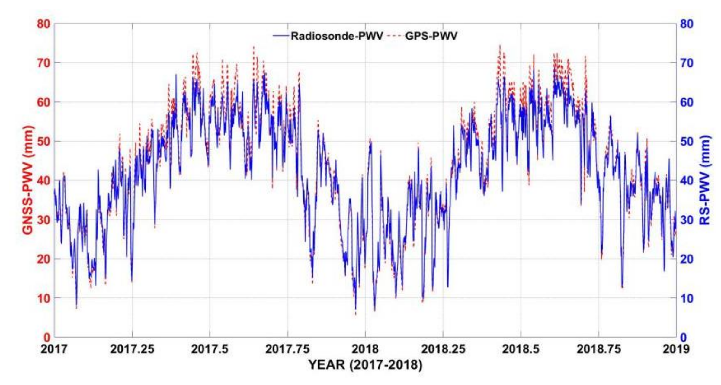
2.2.2. Evaluation of GNSS-PWV

In this section, PWVs derived from the radiosonde (named RS-PWV in this study) were used as the reference to evaluate the accuracy of GNSS-PWVs obtained at the HKSC station since this station is the closest to the radiosonde site, with a 2.9 km horizontal distance and a 3.8 m height difference. The two-year (2017–2018) sounding data containing 1430 radiosonde profiles were acquired from the Integrated Global Radiosonde Archive (IGRA), which is the largest and most comprehensive dataset of quality-assured sounding profiles from 1500 globally distributed stations [81]. Although these data have been gone through rigorous quality control procedures, an additional data pre-processing procedure for gross errors detection was carried out for the 1430 profiles with the following steps:
  • To ensure the density of pressure levels in each profile, if the difference in the pressure levels of any two adjacent layers exceeded 200 hPa, then the profile was excluded.
  • If the pressure levels in each profile missed any of the following levels:
    (a)
    The mandatory levels specified by WMO;
    (b)
    The significant levels suggested by the US National Weather Service (NWS); then the profile was excluded [82].
After the above two steps were examined, 24 profiles were identified and rejected from the initial 1430 profiles, and the remaining 1406 profiles were used as the reference for the evaluation of GNSS-PWV.
RS-PWV was obtained through the following integral [69]:
W = 1 g   p 1 p 2 x d p
where W is the PWV (mm); p1 and p2 are the surface and top pressure levels (Pa) in the profile, respectively; g is the gravitational acceleration; x is the mixing ratio (g/kg) and:
x = 0.622 × e p e
where p is the measured pressure level (in Pa) and e is the pressure of water vapor (in Pa).
Since the sounding balloons are launched only twice per day at 00:00 and 12:00 UTC, the temporal resolution of the RS-PWV time series was much lower than that of GNSS-PWV (1 h vs. 12 h). As a result, only the two hourly GNSS-PWV values (at 00:00 and 12:00 UTC) per day could be validated, which means a total of 1406 pairs of GNSS-PWVs were evaluated, see Figure 2 for the result.
The two PWV time series showed similar temporal variation trends, and the GNSS-PWVs were slightly larger than the RS-PWVs in general. For an overall performance assessment, the statistics including bias, root mean square (RMS) error and correlation coefficient (r) between the two-time series were also calculated (see Table 2 for results) using the following formulas:
b i a s = i = 1 n Y i Y i / n
R M S = i = 1 n Y i Y i 2 / n
r = i = 1 n Y i Y i ¯ × Y i Y i ¯ i = 1 n Y i Y i ¯ 2 × i = 1 n Y i Y i ¯ 2
where the subscription i is the index of the element in the sample data; Y i and Y i are the i-th GNSS-PWV and RS-PWV values, respectively; Y i ¯ and Y i ¯ are the means of the two sets of sample data; n is the number of the samples.
The RMS and bias of 2.18 mm and 1.23 mm manifested a good agreement between both PWV results. As suggested by the EUMETNET EIG GNSS water vapor program [83], the threshold for the accuracy of PWV for meteorological research is 3 mm; thus, the result is acceptable for the meteorological community and consistent with previous studies [58,69,84]. Therefore, in this study, GNSS-PWVs were used to develop a new model for the monitoring of water vapor variation for weather prediction.

2.3. Methods for Determining Thresholds and Evaluating Prediction Results

2.3.1. Criteria for Determining Thresholds and Evaluating of Prediction Results

From comparisons of historical long-term PWV time series against precipitation records over the same period of time, some researchers found that when the values of PWV, PWV variation and rate of PWV variation reached a fixed value, the probability of precipitation would be significantly increased [47,48,49,50]. The fixed value is the so-called precipitation threshold. Different thresholds lead to different prediction results. Theoretically, a larger threshold tends to result in a larger number of omissive predictions, while a smaller threshold often leads to a larger number of misdiagnosis predictions; hence, it is of great importance to determine an optimal threshold value for a better prediction result. Previously, empirical thresholds from a given data range were used in model construction [49,57]. In this study, the standard 2 × 2 contingency table for weather prediction proposed by Doswell and Flueck [85], as shown in Table 3, for its elements and associated dichotomous prediction, was used to determine and validate the threshold. If a predicted result is the same as the truth about the precipitation, then the prediction is a correct prediction. A correct prediction can be resulted from two scenarios, which are denoted by n11 or n22 (see the table for explanations); the other two cases are misdiagnosis prediction and omissive prediction, denoted by n12 and n21, respectively.
Of the above four notations, three were employed by Donaldson et al. [86] to define various criteria for the validation of prediction results, such as the critical success index (CSI), probability of detection (POD) and false alarm rate (FAR), see their formulas below, which have been also applied elsewhere in weather prediction [87,88].
C S I = n 11 / n 11 + n 12 + n 21
P O D = n 11 / n 11 + n 21
F A R = n 12 / n 11 + n 12
Although the POD and FAR are simple and widely used in previous studies, they may result in overpredictions or omissive predictions [89]. Thus, these two criteria are often used as complements to the CSI score for meteorological applications since the CSI score correlates well with a precipitation event. Algorithmically, the CSI is a function of both POD and FAR, according to Equations (12)–(14). This is the reason for this study to use the CSI score as the criterion in the determination of the threshold, and all the three scores were used in the evaluation of prediction results.

2.3.2. Threshold Determination Based on CSI

Since the evolution and occurrence of heavy precipitation is closely related to the type or feature of local climate and may have a certain seasonal pattern [2,34,69], in this study, the optimal set of thresholds for the five predictors for each summer month were determined based on the sample data of PWV time series and precipitation records at the three pairs of co-located stations (listed in Table 1) of the month over the period 2010–2017. The procedure for the determination of any of the five thresholds based on the criterion of CSI is as follows:
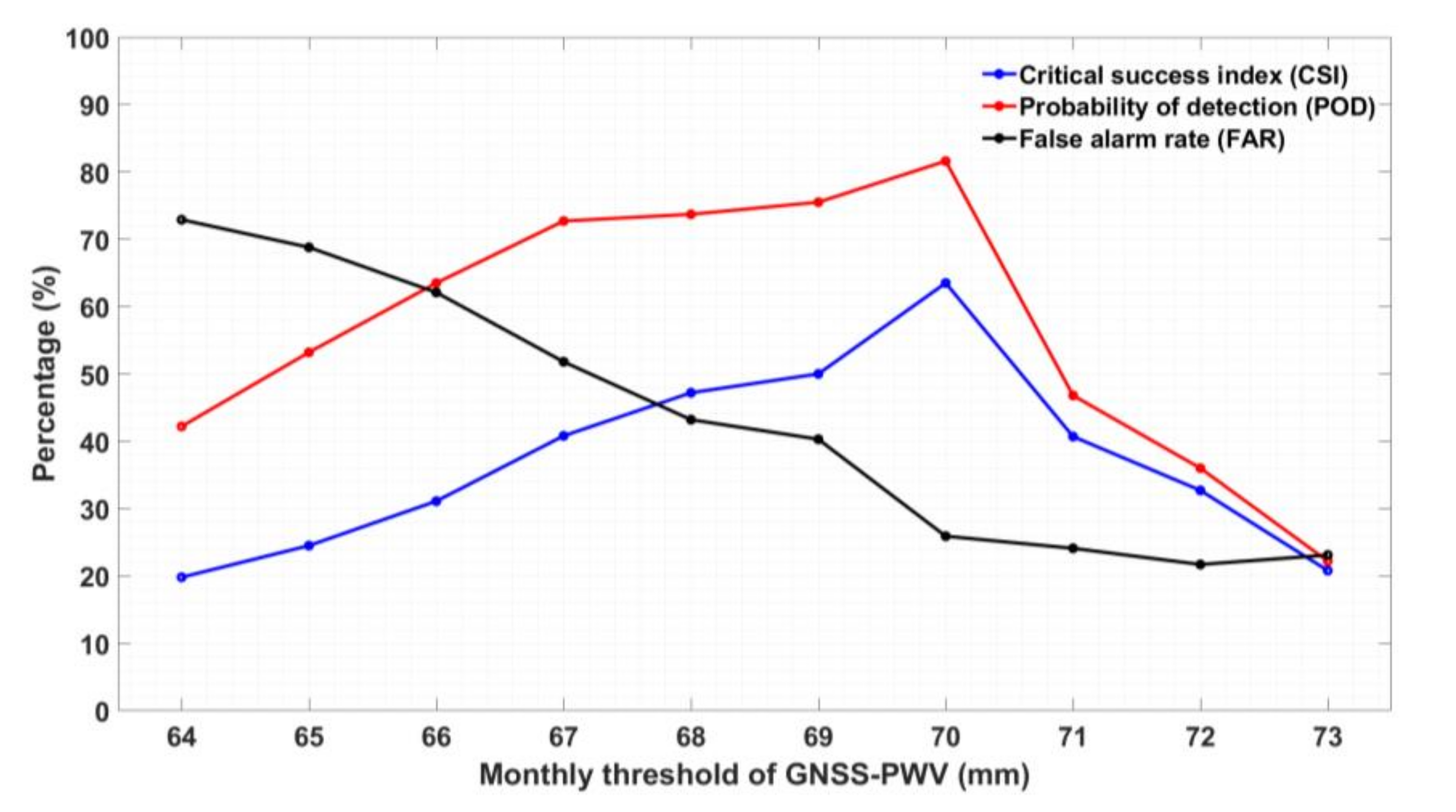
  • A set of candidate threshold values were selected by examining the sample PWV values and the hourly precipitation records in each of the summer months. For example, for the month of June at the HKSC-KP stations, all the GNSS-PWV values (in June from 2010 to 2017) were found in the range 64–73 mm; thus, a set of integer values from this range were taken as candidate threshold values (see the left column in Table 4).
  • Based on the above candidate values and the sample data in the month, n11, n12 and n21 (in Table 3) were counted; then, the candidate’s CSI score was calculated using Equation (12). Table 4 lists the prediction results, including the CSI, POD and FAR scores, resulting from each candidate threshold, and Figure 3 shows the same results, merely for easy comparisons.
  • The candidate that led to the highest CSI score was determined as the optimal threshold. Since the highest CSI score was resulting from the threshold value of 70, 70 was determined as the optimal threshold for the month of June.
From the POD and FAR scores shown in Figure 3, we can see that the threshold of 70 mm also resulted in the maximum POD score and a FAR score close to the minimum. This means the threshold of 70 mm led to the optimal result in terms of all the three scores. Comparing this prediction results with previous studies (the FAR score reported in [49] was 81.7%), the new model’s FAR score was reduced by about 55%, and both correct prediction rates were similar (81.6% vs. 82.7%).

2.3.3. Impact of Different-Length Samples on Determined Thresholds

As suggested by Zhao et al. [50], the thresholds determined based on different-length sample data may be different. To investigate this, PWV times series of different numbers of years, every two years from 2 years (2016–2017) to 8 years (2010–2017), obtained in June at the HKSC-KP station and all precipitation events in June within the specified years were used to obtain the CSI score—the prediction result from the sample data. It is noted that the candidate threshold values were the same as that in Table 4, and the procedure used to obtain the CSI score was the same as the one introduced in the previous section. Results can be seen in Table 5.
It can be seen from Table 5 that the candidate thresholds that resulted in the largest CSI scores were either 70 or 71 mm; and all the CSI scores were above 50 mm; the maximum value was 63.5 mm, which was from the 8-year samples. Although the performance resulting from 71 mm was better based on 2- to 3-year samples, with the increase in time length to 8 years, 70 mm seemed to be more valid and significantly outperformed other candidate thresholds, and thus, it was regarded as the optimal threshold. As a result, the criterion of CSI and eight-year sample data were adopted to determine the optimal set of thresholds for the new model proposed in this study.

3. Relationship between PWV Variation and Heavy Precipitation
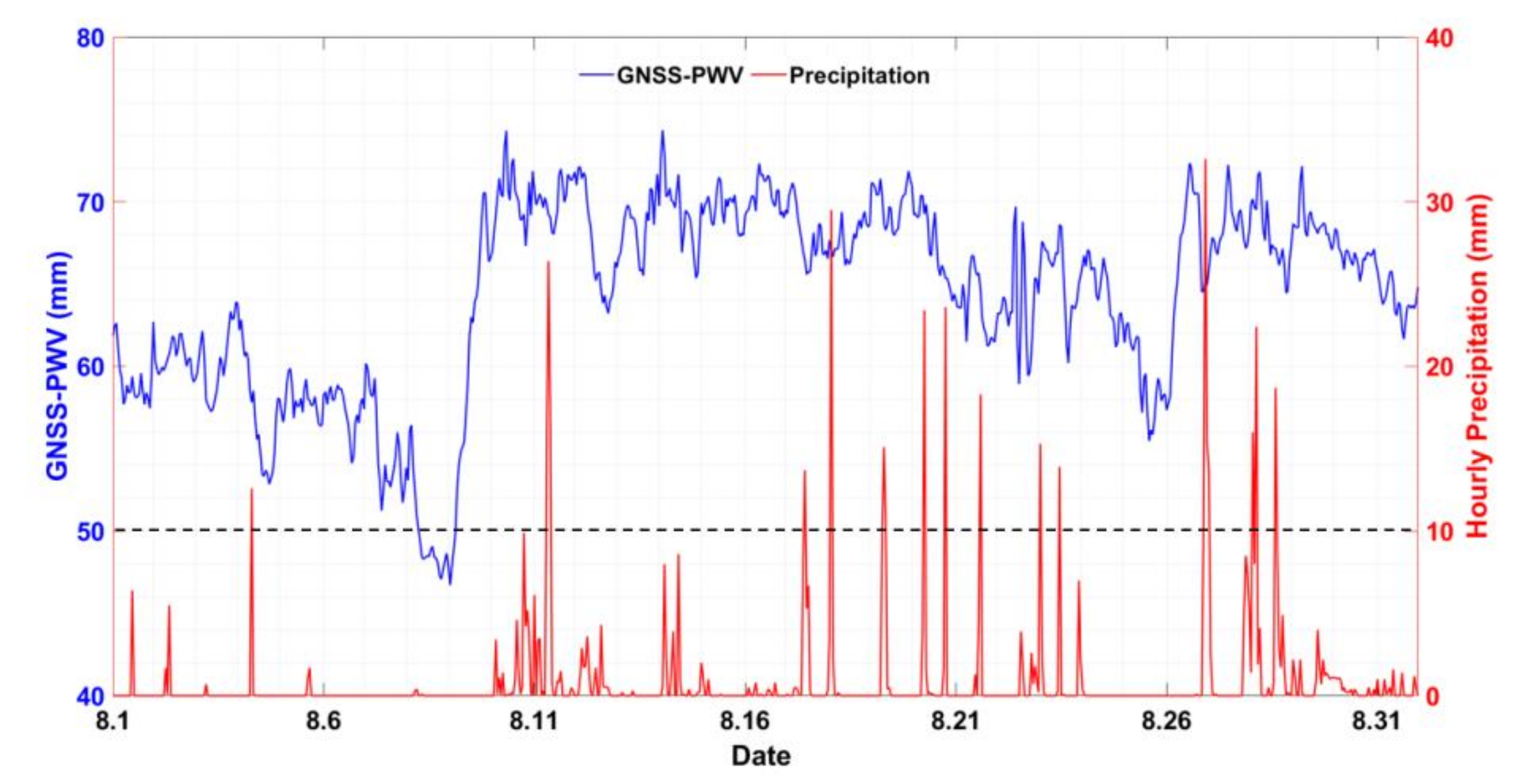
3.1. Overview

In this section, the relationship between the temporal variation in GNSS-PWV and heavy precipitation were analyzed for the potential of using GNSS-PWV derived predictors to predict heavy precipitation. Several studies for different regions have confirmed that PWV correlates well with the occurrence of precipitation [8,49,56], especially in the case of heavy precipitation [36,41,44]. Li et al. [90] stated that PWV significantly increases nearly 2–6 h prior to precipitation, and the same phenomenon was found by Zhao et al. [57]. Zhang et al. [68] claimed that a large increase in PWV was observed 8–10 h prior to some intense precipitation. Liu et al. [91] also found that when a PWV value is above 25 mm and an increase in PWV is above 5 mm, the probability of precipitation is nearly 50% within the region.
In this study, GNSS-PWV data from station HKSC were used to further analyze the spatial and temporal correlation between and the onset of heavy precipitation events in the Hong Kong region. Hourly GNSS-PWV and the corresponding hourly precipitation records obtained from its co-located weather station (KP) over the 1-month period of August in 2018 are shown in Figure 4.
Figure 4 indicates strong consistency between PWV variation and heavy precipitation events. Most heavy precipitation events occur after the PWV peak value is reached. During the evolution process of most heavy precipitation events, is seems that the PWV value is probably to start to increase rapidly till reaching a relatively larger value, then starts to decrease rapidly prior to the heavy precipitation. Comparing the PWV time series and precipitation records in August, 2018, we found that heavy precipitation most happened about 7.31 h after the PWV value reached its peak. In addition, the sharp drop in the PWV time series started from about 4.38 h prior to the following heavy precipitation in this month. For example, the heavy precipitation happened on the 11th day, caused by the tropical severe storm “Bebinca”, clearly depicted the evolution of a heavy precipitation event. As shown in Figure 4, PWV rapidly increased from 46.72 mm to the peak value of 74.34 mm within 20 h; then, it started to sharply decrease to 68.89 mm in the following 8 h; then, it fluctuated around 69 mm until the precipitation rate reached its maximum value of over 25 mm/h. In contrast, when the heavy precipitation stopped, PWV decreased to the minimum of 63.21 mm and then fluctuated around 65 mm or so until the following precipitation event came. This phenomenon and process were found common to almost all heavy precipitation events.

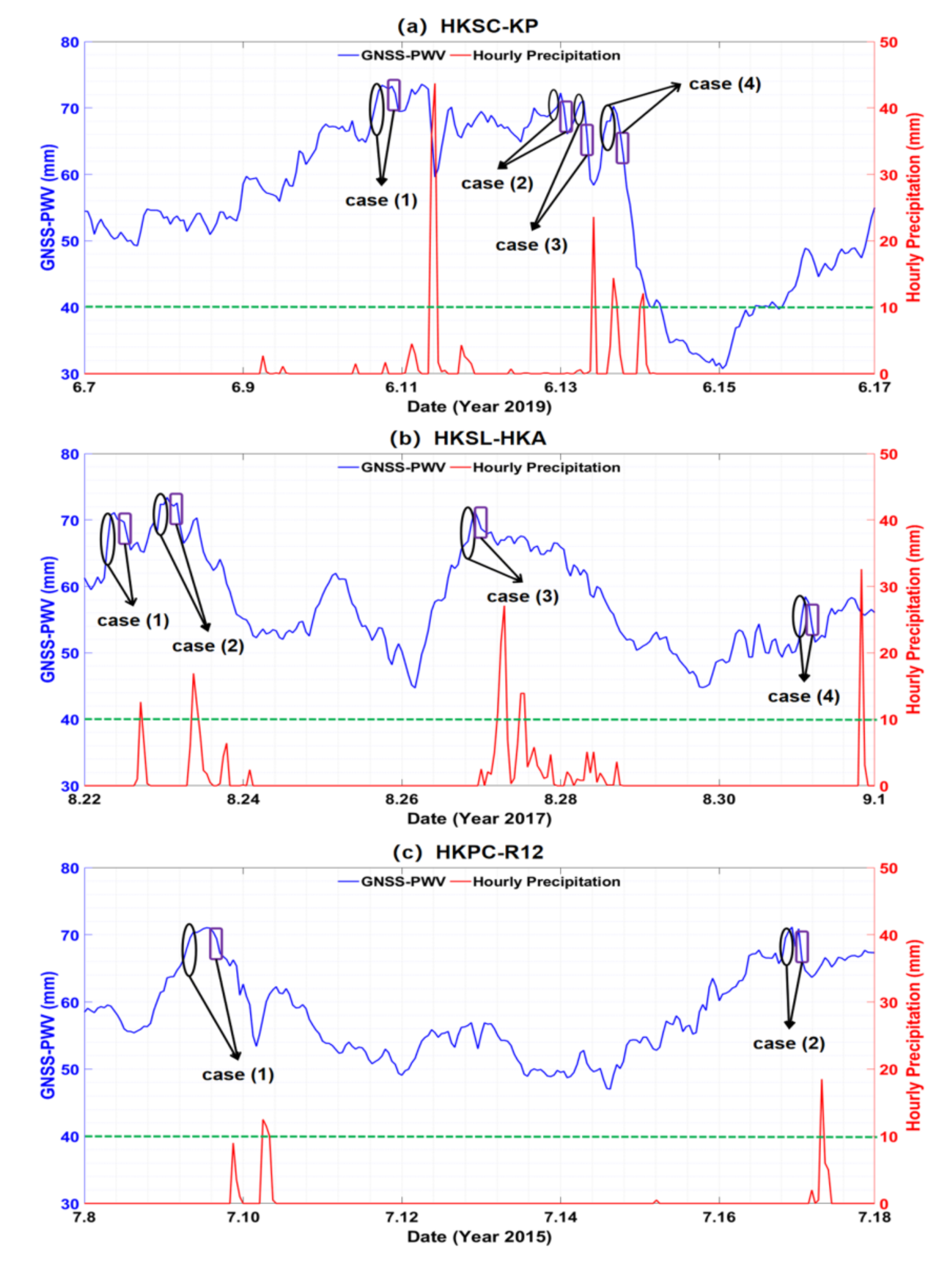
3.2. PWV Variation before the Onset of Heavy Precipitation

The above analysis indicates that the temporal variation in PWV reflects the possibility of heavy precipitation to some extent. When PWV reaches a peak value and the value must be sufficiently large, heavy precipitation is most likely to occur [92]. Therefore, not all GNSS-PWV peaks indicate an arrival of heavy precipitation [45,48,49,50]. Other dynamical factors, a myriad of atmospheric parameters [54,61] and the microphysics of clouds and precipitation [64] also affect the formation of heavy precipitation. Previous studies only use predictors derived from the ascending trend of PWV for precipitation prediction, i.e., the descending trend after PWV reaches a certain peak value is not considered [49,55,57], although the descending trend may also contain information indicating the probability of heavy precipitation.

3.2.1. Formation of Heavy Precipitation

Generally, prior to heavy precipitation, there is a strong water vapor transport, presented in the form of a large increase in PWV, which have been proved in several studies. This is followed by a convergence upward motion process, during which water vapor condenses into cloud droplets. A sharp decrease in PWV indicates the diffusional and collisional growth of cloud and precipitation particles. Finally, with the growth of cloud droplets, the cloud droplets fall as raindrops, i.e., heavy precipitation [64,65,93]. Several researchers have reported this phenomenon, e.g., Van Bealen et al. [8] stated that water vapor decreased sometime before the onset or reinforcement of precipitation and proposed to use the process of water vapor condensation to explain this phenomenon. Madhulatha et al. [66] reported a relative decrease in GNSS-PWV 3 h prior to the storm development. Barindelli et al. [67] observed a steep decrease of 5–10 mm/h in the PWV time series in response to heavy precipitation. Zhang et al. [68] and Yao et al. [49] claimed that a sharp drop in PWV coincided with the passing of extreme precipitation. Benevides et al. [48] and Jones et al. [38] also found severe rain events happened several hours after the PWV value reached the peak. In this study, a comparison of GNSS-PWV time series at HKSC and precipitation records at KP, i.e., a pair of co-located GNSS/weather stations, during the period 2010–2019 was conducted. From the comparison, we found that in more than 94% heavy precipitation cases, prior to heavy precipitation, PWV experienced a rapid increase before reaching a peak value and then considerably decreased.

3.2.2. PWV Variation Prior to Heavy Precipitation

To investigate PWV variation before the onset of heavy precipitation, hourly GNSS-PWV and precipitation records obtained from the three pairs of co-located stations (Section 2.1): HKSC-KP, HKSL-HKA, and HKPC-R12 over the three 10-day periods of 7–16 June 2019, 22–31 August 2017, and 8–17 July 2015, respectively, are shown in Figure 5 for three case studies.
To further investigate the potential of using the descending trend in GNSS-PWV time series for heavy precipitation prediction, apart from the three predictors used in existing methods, two additional predictors—PWV decrement and rate of PWV decrement were introduced for the new model proposed in this study. Detailed definitions of all these five predictors can be found in Table 6, and the additional two parameters used in calculating the two factors of ‘rate of PWV increment’ and ‘rate of PWV decrement’ can be found in the last row of the table. It is noted that the notations “/” and “−” used in the table denote “division” and “subtraction”, respectively.
According to the definitions, the two new predictors, PWV decrement and its rate, can be obtained for every epoch (hour). To obtain a better and convincing predictor on account of the formation process of heavy precipitation stated above, the maximum values of PWV decrement and rate of PWV decrement during the descending period of PWV before a heavy precipitation event were selected for analysis and prediction. Based on the definitions in Table 6, the values of four predictors before the several heavy precipitation events shown in Figure 5 were calculated and the results are given in Table 7.
It can be seen from Table 7 that the values of PWV increment and rate of PWV increment were large prior to heavy precipitation. Moreover, the maximum PWV decrement and the maximum rate of PWV decrement were rather evident, compared to the two predictors derived from the ascending trend, and the maximum rate of PWV decrement even reached 5.85 mm/h in case 3 at the HKSC station. As stated in [55], a saturation threshold value for heavy precipitation highly correlates with temperature, and the threshold value increases with the increase in temperature in most cases, meaning that it is very difficult to predict precipitation accurately if only one predictor derived from PWV time series is used in the prediction. It was also found from case 4 at the HKSL-HKA stations that when heavy precipitation occurred, GNSS-PWV values were relatively small, but both the rates of PWV increment and decrement were large. This result suggests that considering both the ascending and the descending trends in PWV time series in heavy precipitation prediction is more effective than the prediction model that is only based on the PWV value or predictors derived from the ascending trend.

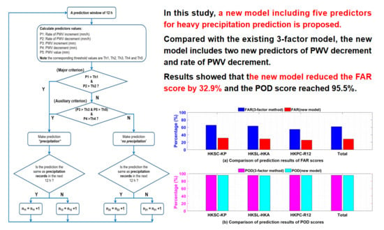
4. Determination and Testing of Five Thresholds for New Model

The key to heavy precipitation prediction is to reduce the false alarm rate under the premise that a high-accuracy prediction rate is ensured. In this section, the new five-predictor model for reducing the number of misdiagnosis predictions was developed, i.e., the optimal set of thresholds for the five predictors were determined. The performance of the new model was evaluated using the predictions resulting from these thresholds and the criteria proposed in Section 4.2.1.

4.1. Determination of Optimal Set of Thresholds

As previously discussed, the first three predictors (see Table 6) are the same as the ones used in the existing three-factor method. In Section 2.3.2, the procedure for determining the optimal threshold for the predictor of PWV value (in June) is presented, for an example. This procedure is also applicable for the predictors of PWV increment and rate of PWV increment. The other two predictors—PWV decrement and rate of PWV decrement, which are included in the new model, were obtained from a different procedure. They were based on the pair of hourly GNSS-PWV values at two consecutive hours in the descending trend of the PWV time series. In addition, from the investigation results in Section 2.3.3, the eight-year sample data resulted in the highest CSI score; thus, the sample data in the summer months over the 8-year period 2010–2017 at the three pairs of co-located stations were used as the samples in the determination of the optimal thresholds for the five predictors, using the same procedure. The results are listed in Table 8, which will be used to test the precipitation prediction in the next section for the performance evaluation of the new model.

4.2. Testing of New Model

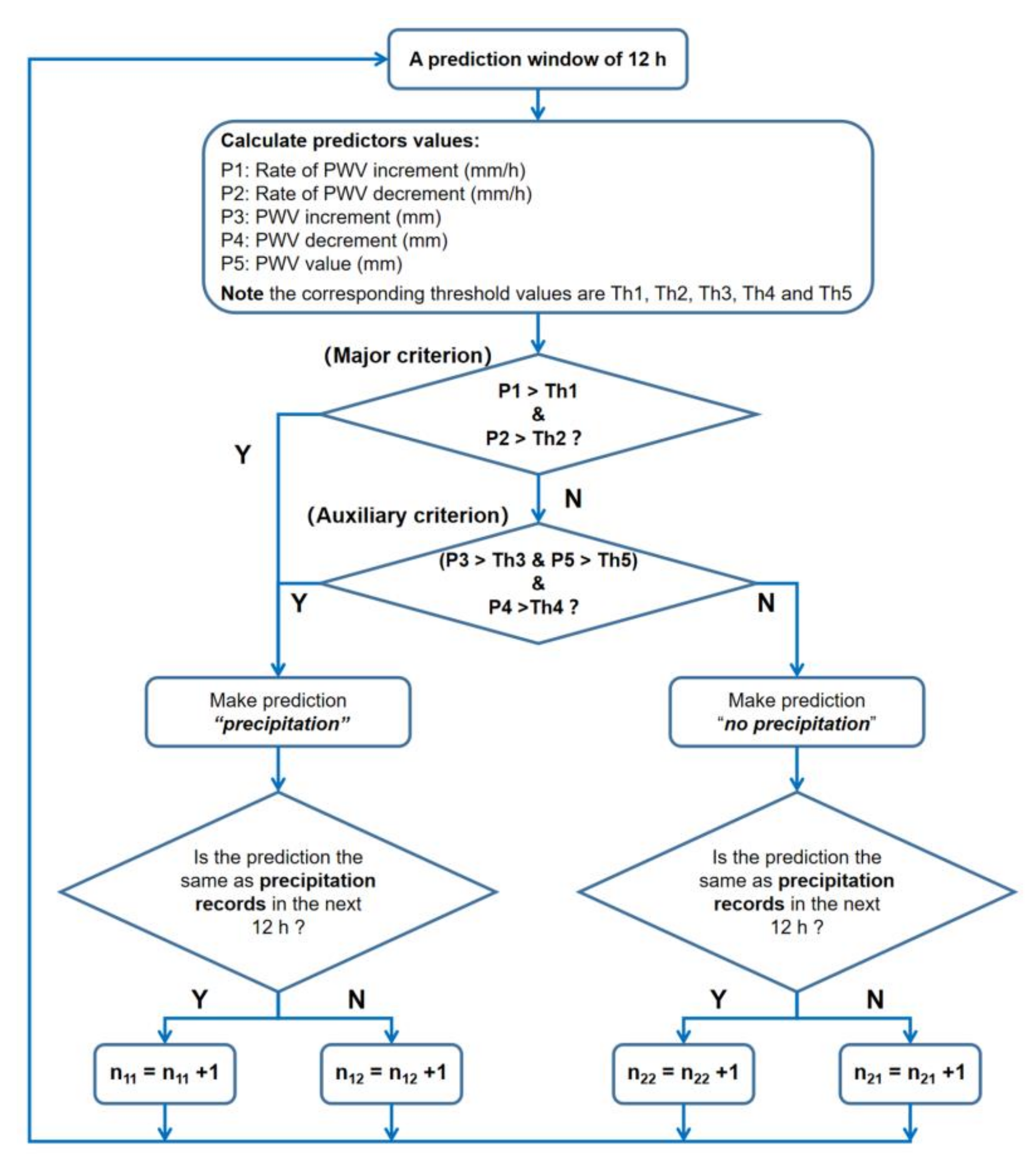
4.2.1. Criteria Determined for Heavy Precipitation Prediction

The criteria used to predict heavy precipitation and evaluate prediction results are often different. For example, the rate of PWV variation was used as the major predictor for precipitation prediction in the three-factor method. However, several other studies stated that the maximum PWV value plays the most important role in precipitation prediction [46,55]. In this study, the combination of the rates of PWV increment and decrement was defined as the major criterion, as suggested by Manandhar et al. [55] that in a temperate or sub-tropical region, the rate of PWV variation is the most important factor for precipitation prediction. To further investigate this and evaluate the predictions resulting from the use of the criteria proposed for the new model, a comparison between the performances resulting from the criteria of the maximum PWV value and the new criteria based on the data at the HKSC-KP station in the summer months during 2010–2019 was performed. Results showed that among a total of 240 heavy precipitation events, 78.8% of them occurred with large rates of PWV increment (above 1.1 mm/h) and decrement (above 1.2 mm/h), while only 55% of them occurred with the maximum PWV reaching their respective thresholds. Therefore, it seems that, for a city like Hong Kong, which is in a sub-tropical region, the rapid increment and decrement in PWV have a larger impact on the occurrence of heavy precipitation than the maximum PWV value. This result has verified the effectiveness of using the combination of the rates of PWV increment and decrement as the major criterion for heavy precipitation prediction proposed for the new model. The procedure for applying the major criterion, along with an auxiliary criterion, to making predictions of heavy precipitation will be elaborated in the following section.

4.2.2. Procedure for New Model Testing
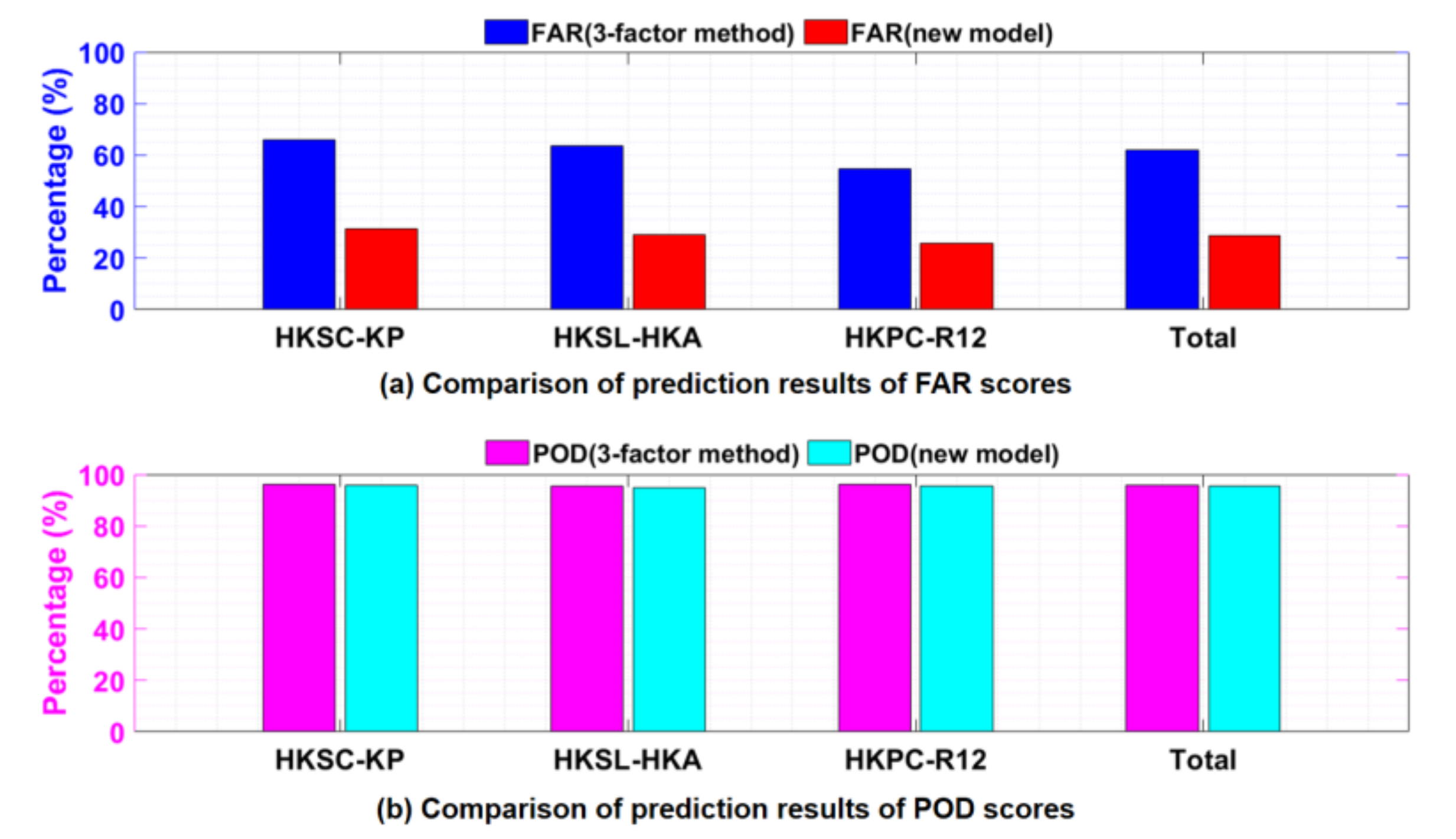
Of the five predictors contained in the new model, two predictors were used as the group for the major criterion, as previously discussed. Similarly, the group of the other three predictors were defined as the auxiliary criterion used to predict precipitation. A prediction of “precipitation” would be made only in the case that the two predictors for the major criterion in the sliding window of 12 h were both above their thresholds; otherwise, a prediction of “no precipitation” would be made. In the case that “no precipitation” was made based on the major criterion, then the auxiliary criterion was further examined, and a prediction of “precipitation” would be made if all the three predictors were above their respective thresholds. The prediction results were validated using the heavy precipitation records in the period of the next 12 h as the reference. For example, when a prediction of “precipitation” was made and a precipitation really happened within the next 12-h window, then the prediction was validated as a correct prediction; see the flowchart illustrated in Figure 6 for the procedure of using the two criteria to make a prediction and the validation of the prediction result. It should be noted that the order of the five predictors shown in the figure is different from that in other tables, due to the grouping of the five predictors for the two new criteria.
After all the steps shown in the flowchart were carried out, the POD and FAR scores can be obtained from Equations (13) and (14) based on the numbers of the correct, omissive and misdiagnosis predictions, respectively.

4.2.3. Results

In this section, the predictions made for each summer month in 2018 and 2019 resulting from the optimal set of thresholds determined for the five predictors in Section 4.1 and using the procedure presented in Figure 6 are shown in Table 9.
As shown in the last column in the table, the POD and FAR scores were 95.5% and 28.9%, respectively. From the statistics of the correct predictions, 189 out of 198 heavy precipitation events were correctly predicted with a lead time of 5.15 h. It is noted that large rainfall refers to at least 5 mm hourly rainfall, according to the previous studies [49,57]. This is not the same as the definition by WMO, which was adopted in this study. To make a comparison between the performances of the new model and the 3-factor method, Table 10 shows the prediction results of the 3-factor model based on the same data as that in Table 9 and a clear comparison between the two models’ results is depicted in Figure 7.
It can be seen from the figure that the new model significantly reduced the number of misdiagnosis predictions (77 vs. 346 in Table 9 and Table 10, respectively), which greatly reduced the FAR score calculated from Equation (14). The FAR score of 28.9% resulting from the new model in comparison with 61.8% from the 3-factor method, meaning a 32.9% improvement made by the new model. The POD scores resulting from the two methods were very close (95% vs. 96%). In some cases, all heavy precipitation events were correctly predicted by both methods, meaning a 100% POD score. Furthermore, the 77 misdiagnosis predictions made by the new model were further investigated and it was found that, about 54.5% (42 out of 77) and 23.4% (18 out of 77) of the misdiagnosis predictions were associated with either moderate precipitation (hourly precipitation ranging from 2.5 to 10 mm) or slight precipitation (hourly precipitation ranging from 0.1 to 10 mm) occurred within the next 12-h prediction window, while only 17 misdiagnosis predictions had no corresponding precipitation occurring. In general, the improvements in prediction results from the new model were significant.

5. Discussion

A strong correlation between GNSS-PWV and heavy precipitation is one of the most important preconditions for using GNSS-PWV time series to predict heavy precipitation. In this study, from an investigation of the relationship between GNSS-PWV time series and heavy precipitation records in several case studies over the above three stations, a noticeable increase followed by a steep drop in the GNSS-PWV time series was found several hours prior to the onset of most heavy precipitation events. Based on this finding, hourly GNSS-PWVs and precipitation records over three co-located GNSS/weather stations (HKSC-KP, HKSL-HKA and HKPC-R12) in Hong Kong during the 10-year period 2010–2019 were obtained for development and assessment of an improved 5-preditor model for short-term heavy precipitation prediction. The five predictors proposed in the new model contained the three commonly used predictors, PWV value, PWV increment and rate of the PWV increment, which are derived from the ascending trend of the PWV time series; the two new predictors, PWV decrement and rate of the PWV decrement, are proposed for the first time in this study for reducing the numbers of misdiagnosis predictions and the FAR scores while a better POD score is also ensured. Since different sets of thresholds selected for the five predictors result in different predictions, the optimal set of thresholds was determined using the common method that uses the CSI score derived from a contingency table as the major criterion for weather prediction in this study.
As the inherent relationship between PWV and heavy precipitation is complex, which is difficult to be fully revealed by a threshold-based model. In this study, we analyzed whether the proposed five predictors derived from PWV time series met the requirement (threshold) for precipitation; however, the accuracy of the precipitation prediction is expected to be improved if the PWV values are combined with other relevant meteorological parameters. In addition, the integral nature of PWV could only reflect the spatiotemporal variations of water vapor to some extent; however, the water vapor tomography has been proved to be a mature technique to obtain water vapor profile for monitoring the dynamic evolution of water vapor in the life cycle of precipitation events. Therefore, our future work will be focusing on also containing tomography-based vertical profiles and various types of atmospheric data such as temperature, pressure, relative humidity, wind, solar radiation, etc., in the modelling for the improvements in the accuracy of precipitation prediction.

6. Conclusions

In this study, based on a strong consistency between PWV and heavy precipitation, a new model containing five predictors for short-term heavy precipitation prediction was developed using the data of hourly GNSS-PWV time series and precipitation records over the 8-year period 2010–2017. The optimal set of thresholds for the five predictors in each of the summer months were determined based on the indices of CSI scores and the data of hourly GNSS-PWV and precipitation records in the same month during the 8-year period, 2010–2017 at the aforementioned three stations. This set of optimal thresholds of the five predictors were then used in the testing of the new model. In the testing procedure, the five predictors were divided into two groups, named two criteria—a major criterion and an auxiliary criterion—which were successively examined for a precipitation prediction. Then, the new model was tested using the hourly GNSS-PWV in the summer months of 2018 and 2019, and the prediction results were compared with the hourly precipitation records in the period of the next 12 h for the validation of the model. Results showed that, of the 198 heavy precipitation events, 189 events were successfully predicted with a lead time of 5.15 h. The new model led to a 28.9% FAR score, in comparison with 61.8% resulting from the commonly used three-factor model, meaning a 32.9% improvement made by the new model, while under the premise of a significant decrease in the FAR scores, the POD scores resulting from the two methods were comparable at a high level (95.5% vs. 96%). These results of this study suggest it is promising to use the new model proposed to obtain better prediction results for heavy precipitation events in near real-time.

Author Contributions

Conceptualization, H.L.; methodology, H.L., X.W. and K.Z.; validation, H.L., X.W. and S.W.; formal analysis, H.L. and X.W.; resources, X.W., J.Z., S.Z., X.C., C.Q. and L.L.; software, H.L. and M.X.; writing—original draft preparation, H.L.; writing—review and editing, X.W., S.W. and K.Z.; supervision, X.W., K.Z. and S.W.; funding acquisition, H.L., X.W. and K.Z. All authors have read and agreed to the published version of the manuscript.

Funding

This research was supported by the Future Scientists Program of China University of Mining and Technology, grant number 2020WLKXJ053, and the Postgraduate Research & Practice Innovation Program of Jiangsu Province, grant number KYCX20_1835.

Acknowledgments

The authors would like to thank the IGS for providing precise GPS data, the Hong Kong Observation for providing hourly precipitation data, the National Climate Data Center for providing the Integrated Global Radiosonde Archive, and the CAS Pioneer Hundred Talents Program for providing support during the whole research process.

Conflicts of Interest

The authors declare no conflict of interest.

References

  1. Li, P.W.; Wong, W.K.; Cheung, P.; Yeung, H.Y. An overview of nowcasting development, applications, and services in the Hong Kong Observatory. J. Meteorol. Res. 2014, 28, 859–876. [Google Scholar] [CrossRef]
  2. Chen, B.; Liu, Z.; Wong, W.K.; Woo, W.C. Detecting water vapor variability during heavy precipitation events in Hong Kong using the GPS tomographic technique. J. Atmos. Ocean. Tech. 2017, 34, 1001–1019. [Google Scholar] [CrossRef]
  3. Foster, J.; Bevis, M.; Chen, Y.L.; Businger, S.; Zhang, Y. The Ka ’u storm (November 2000): Imaging precipitable water using GPS. J. Geophys. Res. 2003, 108, 4585. [Google Scholar] [CrossRef]
  4. Seko, H.; Nakamura, H.; Shoji, Y.; Iwabuchi, T. The Meso-γ scale Water Vapor Distribution Associated with a Thunderstorm Calculated from a Dense Network of GPS Receivers. J. Meteorol. Soc. Jpn. 2004, 82, 569–586. [Google Scholar] [CrossRef] [Green Version]
  5. Chiang, K.W.; Peng, W.C.; Yeh, Y.H.; Chen, K.H. Study of alternative GPS network meteorological sensors in Taiwan: Case studies of the plum rains and typhoon Sinlaku. Sensors 2009, 9, 5001–5021. [Google Scholar] [CrossRef] [Green Version]
  6. Moore, A.W.; Small, I.J.; Gutman, S.I.; Bock, Y.; Dumas, J.L.; Fang, P.; Laber, J.L. National weather service forecasters use GPS precipitable water vapor for enhanced situational awareness during the southern California summer monsoon. Bull. Am. Meteorol. Soc. 2015, 96, 1867–1877. [Google Scholar] [CrossRef]
  7. Muller, C.J.; Back, L.E.; O’Gorman, P.A.; Emanuel, K.A. A model for the relationship between tropical precipitation and column water vapor. Geophys. Res. Lett. 2009, 36. [Google Scholar] [CrossRef]
  8. Van Baelen, J.; Reverdy, M.; Tridon, F.; Labbouz, L.; Dick, G.; Bender, M.; Hagen, M. On the relationship between water vapour field evolution and the life cycle of precipitation systems. Q. J. R. Meteorol. Soc. 2011, 137, 204–223. [Google Scholar] [CrossRef] [Green Version]
  9. Brettle, M.; Galvin, J. Back to basics: Radiosondes: Part 1—The instrument. Weather 2006, 58, 336–341. [Google Scholar] [CrossRef]
  10. England, M.; Schmidlin, F.J.; Johansson, J. Atmospheric Moisture Measurements: A Microwave Radiometer-Radiosonde Comparison. IEEE Trans. Geosci. Remote Sens. 1993, 31, 389–398. [Google Scholar] [CrossRef]
  11. Buehler, S.A.; Kuvatov, M.; John, V.O.; Milz, M.; Soden, B.J.; Jackson, D.L.; Notholt, J. An upper tropospheric humidity data set from operational satellite microwave data. J. Geophys. Res. Atmos. 2008, 113. [Google Scholar] [CrossRef] [Green Version]
  12. Niell, A.E.; Coster, A.; Solheim, F.; Mendes, V.; Toor, P.; Langley, R.; Upham, C.A. Comparison of Measurements of Atmospheric Wet Delay by Radiosonde, Water Vapor Radiometer, GPS, and VLBI. J. Atmos. Ocean. Technol. 2001, 18, 830–850. [Google Scholar] [CrossRef] [Green Version]
  13. Liu, Z.; Wong, M.; Nichol, J.; Chan, P.W. A multi-sensor study of water vapour from radiosonde, MODIS and AERONET: A case study of Hong Kong. Int. J. Clim. 2013, 33, 109–120. [Google Scholar] [CrossRef] [Green Version]
  14. Elliott, W.P. On detecting long-term changes in atmospheric moisture. Clim. Chang. 1995, 31, 349–367. [Google Scholar] [CrossRef]
  15. Wang, H.; He, J.; Wei, M.; Zhang, Z. Synthesis analysis of one severe convection precipitation event in Jiangsu using ground-based GPS technology. Atmosphere 2015, 6, 908–927. [Google Scholar] [CrossRef] [Green Version]
  16. Gui, K.; Che, H.; Chen, Q.; Zeng, Z.; Liu, H.; Wang, Y.; Zhang, X. Evaluation of radiosonde, MODIS-NIR-Clear, and AERONET precipitable water vapor using IGS ground-based GPS measurements over China. Atmos. Res. 2017, 197, 461–473. [Google Scholar] [CrossRef]
  17. Baker, H.C.; Dodson, A.H.; Penna, N.T.; Higgins, M.; Offiler, D. Ground-based GPS water vapour estimation: Potential for meteorological forecasting. J. Atmos. Sol.-Terr. Phys. 2001, 63, 1305–1314. [Google Scholar] [CrossRef]
  18. Brenot, H.; Neméghaire, J.; Delobbe, L.; Clerbaux, N.; De Meutter, P.; Deckmyn, A.; Van Roozendael, M. Preliminary signs of the initiation of deep convection by GNSS. Atmos. Chem. Phys. 2013, 13, 5425–5449. [Google Scholar] [CrossRef] [Green Version]
  19. Askne, J.; Nordius, H. Estimation of Tropospheric Delay for Microwaves from Surface Weather Data. Radio Sci. 1987, 22, 379–386. [Google Scholar] [CrossRef]
  20. Elgered, G.; Davis, J.; Herring, T.; Shapiro, I. Geodesy by radio interferometry: Water vapor radiometry for estimation of the wet delay. J. Geophys. Res. Atmos. 1991, 96, 6541–6555. [Google Scholar] [CrossRef]
  21. Bevis, M.; Businger, S.; Herring, T.; Rocken, C.; Anthes, R.; Ware, R. GPS Meteorology: Remote Sensing of Atmospheric Water Vapor Using the Global Positioning System. J. Geophys. Res. Atmos. 1992, 97, 15787–15801. [Google Scholar] [CrossRef]
  22. Bevis, M.; Businger, S.; Chiswell, S.; Herring, T.; Anthes, R.; Rocken, C.; Ware, R. GPS Meteorology: Mapping Zenith Wet Delays onto Precipitable Water. J. Appl. Meteorol. 1994, 33, 379–386. [Google Scholar] [CrossRef]
  23. Rocken, C.; Hove, T.; Johnson, J.; Solheim, F.; Ware, R.; Bevis, M.; Chiswell, S.; Businger, S. GPS/STORM-GPS sensing of atmospheric water vapour for meteorology. J. Atmos. Ocean. Technol. 1995, 12, 468–478. [Google Scholar] [CrossRef]
  24. Duan, J.; Bevis, M.; Fang, P.; Bock, Y.; Chiswell, S.; Businger, S.; Rocken, C.; Solheim, F.; Hove, T.; Ware, R.; et al. GPS Meteorology: Direct Estimation of the Absolute Value of Precipitable Water. J. Appl. Meteorol. 1996, 35, 830–838. [Google Scholar] [CrossRef] [Green Version]
  25. Yuan, L.; Anthes, R.; Ware, R.; Rocken, C.; Bonner, W.; Bevis, M.; Businger, S. Sensing climate change using the global positioning system. J. Geophys. Res. 1993, 981, 14925–14938. [Google Scholar] [CrossRef] [Green Version]
  26. Rocken, C.; Ware, R.; Hove, T.; Solheim, F.; Alber, C.; Johnson, J.; Bevis, M.; Businger, S. Sensing atmospheric water vapor with the Global Positioning System. Geophys. Res. Lett. 1993, 20, 2631–2634. [Google Scholar] [CrossRef] [Green Version]
  27. Jin, S.; Li, Z.; Cho, J. Integrated water vapor field and multiscale variations over China from GPS measurements. J. Appl. Meteorol. Clim. 2008, 47, 3008–3015. [Google Scholar] [CrossRef]
  28. Nilsson, T.; Elgered, G. Long-term trends in the atmospheric water vapor content estimated from ground-based GPS data. J. Geophys. Res. 2008, 113, D19101. [Google Scholar] [CrossRef] [Green Version]
  29. Wang, X.; Zhang, K.; Wu, S.; He, C.; Cheng, Y.; Li, X. Determination of zenith hydrostatic delay and its impact on GNSS-derived integrated water vapor. Atmos. Meas. Tech. 2017, 10, 2807–2820. [Google Scholar] [CrossRef] [Green Version]
  30. Vedel, H.; Huang, X.Y.; Haase, J.; Ge, M.; Calais, E. Impact of GPS zenith tropospheric delay data on precipitation forecasts in Mediterranean France and Spain. Geophys. Res. Lett. 2004, 31. [Google Scholar] [CrossRef] [Green Version]
  31. Wang, X.; Zhang, K.; Wu, S.; Li, Z.; Cheng, Y.; Li, L.; Yuan, H. The correlation between GNSS-derived precipitable water vapor and sea surface temperature and its responses to El Niño–Southern Oscillation. Remote Sens. Environ. 2018, 216, 1–12. [Google Scholar] [CrossRef]
  32. Le Marshall, J.; Norman, R.; Howard, D.; Rennie, S.; Moore, M.; Kaplon, J.; Lehmann, P. Using global navigation satellite system data for real-time moisture analysis and forecasting over the Australianregion I. The system. J. South. Hemisph. Earth 2019, 69, 161–171. [Google Scholar] [CrossRef]
  33. Gradinarsky, L.P.; Johansson, J.; Bouma, H.; Scherneck, H.-G.; Elgered, G. Climate monitoring using GPS. Phys. Chem. Earth 2002, 27, 335–340. [Google Scholar] [CrossRef]
  34. Jin, S.; Park, J.; Cho, J.-H.; Park, P.-H. Seasonal variability of GPS-derived zenith tropospheric delay (1994–2006) and climate implications. J. Geophys. Res. 2007, 112, D09110. [Google Scholar] [CrossRef]
  35. Rohm, W.; Yuan, Y.; Biadeglgne, B.; Zhang, K.; Le Marshall, J. Ground-based GNSS ZTD/IWV estimation system for numerical weather prediction in challenging weather conditions. Atmos. Res. 2013, 138, 414–426. [Google Scholar] [CrossRef]
  36. Choy, S.; Zhang, K.; Wang, C.S.; Li, Y.; Kuleshov, Y. Remote Sensing of the Earth’s Lower Atmosphere during Severe Weather Events using GPS Technology: A Study in Victoria, Australia. In Proceedings of the 24th International Technical Meeting of the Satellite Division of the Institute of Navigation (ION GNSS 2011), Oregon Convention Center, Portland, OR, USA, 20–23 September 2011; Volume 1, pp. 559–571. [Google Scholar]
  37. Suparta, W.; Zulkeple, S.K.; Putro, W.S. Estimation of thunderstorm activity in tawau, sabah using GPS data. Adv. Sci. Lett. 2017, 23, 1370–1373. [Google Scholar] [CrossRef]
  38. Jones, J.; Guerova, G.; Douša, J.; Dick, G.; de Haan, S.; Pottiaux, E.; van Malderen, R. Advanced GNSS Tropospheric Products for Monitoring Severe Weather Events and Climate; COST Action ES1206 Final Action Dissemination Report; Springer: Berlin/Heidelberg, Germany, 2019; p. 563. [Google Scholar] [CrossRef]
  39. Singh, R.P.; Mishra, N.C.; Verma, A.; Ramaprasad, J. Total precipitable water over the Arabian Ocean and the Bay of Bengal using SSM/I data. Int. J. Remote Sens. 2000, 21, 2497–2503. [Google Scholar] [CrossRef]
  40. Singh, R.P.; Dey, S.; Sahoo, A.K.; Kafatos, M. Retrieval of water vapor using SSM/I and its relation with the onset of monsoon. Ann. Geophys. 2004, 22, 3079–3083. [Google Scholar] [CrossRef] [Green Version]
  41. Champollion, C.; Masson, F.; Van Baelen, J.; Walpersdorf, A.; Chéry, J.; Doerflinger, E. GPS monitoring of the tropospheric water vapor distribution and variation during the 9 September 2002 torrential precipitation episode in the Cévennes (southern France). J. Geophys. Res. Atmos. 2004, 109. [Google Scholar] [CrossRef] [Green Version]
  42. Kedem, B.; Chiu, L.S.; Karni, Z. An analysis of the threshold method for measuring area-average rainfall. J. Appl. Meteorol. 1990, 29, 3–20. [Google Scholar] [CrossRef] [Green Version]
  43. Cheng, M.; Brown, R. Estimation of area-average rainfall for frontal rain using the threshold method. Quart. J. R. Meteorol. Soc. 1993, 119, 825–844. [Google Scholar] [CrossRef]
  44. Kanda, M. Correlation between convective heavy rainfalls and GPS precipitable water. In Proceedings of the International Workshop on GPS Meteorology, Tsukuba, Japan, 14–17 January 2003; pp. 3–12. [Google Scholar]
  45. Shoji, Y. Retrieval of Water Vapor Inhomogeneity Using the Japanese Nationwide GPS Array and its Potential for Prediction of Convective Precipitation. J. Meteorol. Soc. Jpn. 2013, 91, 43–62. [Google Scholar] [CrossRef] [Green Version]
  46. Shi, J.; Xu, C.; Guo, J.; Gao, Y. Real-time GPS precise point positioning-based precipitable water vapor estimation for rainfall monitoring and forecasting. IEEE Trans. Geosci. Remote Sens. 2014, 53, 3452–3459. [Google Scholar]
  47. Yeh, T.K.; Shih, H.C.; Wang, C.S.; Choy, S.; Chen, C.H.; Hong, J.S. Determining the precipitable water vapor thresholds under different rainfall strengths in Taiwan. Adv. Space Res. 2018, 61, 941–950. [Google Scholar] [CrossRef]
  48. Benevides, P.; Catalao, J.; Miranda, P. On the inclusion of GPS precipitable water vapour in the nowcasting of rainfall. Nat. Hazard. Earth Syst. 2015, 15, 2605–2616. [Google Scholar] [CrossRef] [Green Version]
  49. Yao, Y.; Shan, L.; Zhao, Q. Establishing a method of short-term rainfall forecasting based on GNSS-derived PWV and its application. Sci. Rep. 2017, 7, 1–11. [Google Scholar] [CrossRef]
  50. Zhao, Q.; Liu, Y.; Ma, X.; Yao, W.; Yao, Y.; Li, X. An Improved Rainfall Forecasting Model Based on GNSS Observations. IEEE Trans. Geosci. Remote Sens. 2020. [Google Scholar] [CrossRef]
  51. Flores, A.; Ruffini, G.; Rius, A. 4D tropospheric tomography using GPS slant wet delays. Ann. Geophys. 2000, 18, 223–234. [Google Scholar] [CrossRef]
  52. Brenot, H.; Wautelet, G.; Warnant, R.; Nemeghaire, J.; Van Roozendael, M.; Theys, N.; Hurtmans, D. A GPS network for tropospheric tomography in the framework of the Mediterranean hydrometeorological observatory Cévennes-Vivarais (southeastern France). Nat. Hazards Earth Syst. Sci. 2014, 14, 1099–1123. [Google Scholar] [CrossRef] [Green Version]
  53. Manning, T.; Zhang, K.; Rohm, W.; Choy, S.; Hurter, F. Detecting Severe Weather using GPS Tomography: An Australian Case Study. J. Glob. Position. Syst. 2012, 11, 58–70. [Google Scholar] [CrossRef]
  54. Seco, A.; Ramírez, F.; Serna, E.; Prieto, E.; García, R.; Moreno, A.; Cantera, J.; Miqueleiz, L.; Priego, J. Rain pattern analysis and forecast model based on GPS estimated atmospheric water vapor content. Atmos. Environ. 2012, 49, 85–93. [Google Scholar] [CrossRef] [Green Version]
  55. Manandhar, S.; Lee, Y.H.; Meng, Y.S. GPS-PWV Based Improved Long-Term Rainfall Prediction Algorithm for Tropical Regions. Remote Sens. 2019, 11, 2643. [Google Scholar] [CrossRef] [Green Version]
  56. Manandhar, S.; Lee, Y.H.; Meng, Y.S.; Yuan, F.; Ong, J. GPS-Derived PWV for Rainfall Nowcasting in Tropical Region. IEEE Trans. Geosci. Remote Sens. 2018, 56, 4835–4844. [Google Scholar] [CrossRef]
  57. Zhao, Q.; Yao, Y.; Yao, W. GPS-based PWV for precipitation forecasting and its application to a typhoon event. J. Atmos. Sol.-Terr. Phy. 2018, 167, 124–133. [Google Scholar] [CrossRef]
  58. Zhao, Q.; Ma, X.; Yao, Y. Preliminary result of capturing the signature of heavy rainfall events using the 2-d-/4-d water vapour information derived from GNSS measurement in Hong Kong. Adv. Space Res. 2020, 66, 1537–1550. [Google Scholar] [CrossRef]
  59. Łoś, M.; Smolak, K.; Guerova, G.; Rohm, W. GNSS-Based Machine Learning Storm Nowcasting. Remote Sens. 2020, 12, 2536. [Google Scholar] [CrossRef]
  60. Boniface, K.; Ducrocq, V.; Jaubert, G.; Yan, X.; Brousseau, P.; Masson, F.; Champollion, C.; Chery, J.; Doerflinger, E. Impact of high-resolution data assimilation of GPS zenith delay on Mediterranean heavy rainfall forecasting. Ann. Geophys. 2009, 27, 2739–2753. [Google Scholar] [CrossRef]
  61. Liu, Y.; Zhao, Q.; Yao, W.; Ma, X.; Yao, Y.; Liu, L. Short-term rainfall forecast model based on the improved Bp–nn algorithm. Sci. Rep. 2019, 9, 1–12. [Google Scholar] [CrossRef]
  62. Manandhar, S.; Dev, S.; Lee, Y.H.; Meng, Y.S.; Winkler, S. A data-driven approach for accurate rainfall prediction. IEEE Trans. Geosci. Remote Sens. 2019, 57, 9323–9331. [Google Scholar] [CrossRef] [Green Version]
  63. Bonafoni, S.; Biondi, R.; Brenot, H.; Anthes, R. Radio occultation and ground-based GNSS products for observing, understanding and predicting extreme events: A review. Atmos. Res. 2019, 230, 104624. [Google Scholar] [CrossRef]
  64. Pruppacher, H.R.; Klett, J.D. Diffusion Growth and Evaporation of Water Drops and Snow Crystals. In Microphysics of Clouds and Precipitation; Springer: Dordrecht, The Netherlands, 2010; pp. 502–567. [Google Scholar]
  65. Wang, P.K. Physics and Dynamics of Clouds and Precipitation; Cambridge University Press: Cambridge, UK, 2013. [Google Scholar]
  66. Madhulatha, A.; Rajeevan, M.; Venkat Ratnam, M.; Bhate, J.; Naidu, C.V. Nowcasting severe convective activity over southeast India using ground-based microwave radiometer observations. J. Geophys. Res. Atmos. 2013, 118, 1–13. [Google Scholar] [CrossRef] [Green Version]
  67. Barindelli, S.; Realini, E.; Venuti, G.; Fermi, A.; Gatti, A. Detection of water vapor time variations associated with heavy rain in northern Italy by geodetic and low-cost GNSS receivers. Earth Planets Space 2018, 70, 28. [Google Scholar] [CrossRef] [Green Version]
  68. Zhang, K.; Manning, T.; Wu, S.; Rohm, W.; Silcock, D.; Choy, S. Capturing the Signature of Severe Weather Events in Australia Using GPS Measurements. IEEE J. Sel. Top. Appl. Earth Obs. Remote Sen. 2015, 8, 1839–1847. [Google Scholar] [CrossRef]
  69. Liu, Z.; Chen, B.; Chan, S.-T.; Yunchang, C.; Gao, Y.; Zhang, K.; Nichol, J. Analysis and modelling of water vapour and temperature changes in Hong Kong using a 40-year radiosonde record: 1973–2012. Int. J. Clim. 2014, 35, 462–474. [Google Scholar] [CrossRef]
  70. Zhao, P.; Zhou, Z.; Liu, J. Variability of Tibetan spring snow and its associations with the hemispheric extratropical circulation and East Asian summer monsoon rainfall: An observational investigation. J. Clim. 2007, 20, 3942–3955. [Google Scholar] [CrossRef]
  71. Chow, K.C.; Tong, H.W.; Chan, J.C. Water vapor sources associated with the early summer precipitation over China. Clim. Dyn. 2008, 30, 497–517. [Google Scholar] [CrossRef]
  72. Hong Kong Observatory. Observed Climate Change in Hong Kong: Extreme Weather Events. 2016. Available online: http://www.weather.gov.hk/climate_change/obs_hk_extreme_weather_e.htm (accessed on 18 July 2020).
  73. WMO. Guide to Instruments and Methods of Observation, Volume I—Measurement of Meteorological Variables; World Meteorological Organization: Geneva, Switzerland, 2018. [Google Scholar]
  74. Tietze, W.; Domrös, M. The climate of China. GeoJournal. 1987, 14, 265–266. [Google Scholar] [CrossRef]
  75. Hong Kong Observatory. Number of Days with Rainfall Observed at the Hong Kong Observatory Since 1885, Exclude 1940–1946. 2019. Available online: https://www.hko.gov.hk/en/cis/statistic/rf_days.htm (accessed on 29 August 2020).
  76. Rocken, C.; Hove, T.; Ware, R. Near Real-Time GPS Sensing of Atmospheric Water Vapour. Geophys. Res. Lett. 1997, 24, 3221–3224. [Google Scholar] [CrossRef] [Green Version]
  77. Dach, R.; Lutz, S.; Walser, P.; Fridez, P. Bernese GNSS Software; Version 5.2; Astronomical Institute, University of Bern: Berne, Switzerland, 2015. [Google Scholar]
  78. Böhm, J.; Werl, B.; Schuh, H. Troposphere mapping functions for GPS and very long baseline interferometry from European Centre for Medium-Range Weather Forecasts operational analysis data. J. Geophys. Res. Solid Earth 2006, 111. [Google Scholar] [CrossRef]
  79. Saastamoinen, J. Atmospheric Correction for the Troposphere and the Stratosphere in Radio Ranging of Satellites. Geophys. Monogr. 1972, 15, 247–251. [Google Scholar]
  80. Chen, Y. Inversing the content of vapor in atmosphere by GPS observations. Mod. Surv. Mapp. 2005, 28, 3–6. [Google Scholar]
  81. Durre, I.; Vose, R.; Wuertz, D. Overview of the Integrated Global Radiosonde Archive. J. Clim. 2006, 19, 53–68. [Google Scholar] [CrossRef] [Green Version]
  82. Wright, J.M., Jr. Federal Meteorological Handbook No. 3: Rawinsonde and Pibal Obervations; Office of the Federal Coordinator for Meteorology, National Oceanic and Atmospheric Administration: Washington, DC, USA, May 1997. Available online: https://www.ofcm.gov/publications/fmh/FMH3/00-entire-FMH3.pdf (accessed on 31 August 2020).
  83. Offiler, D.; Jones, J.; Bennit, G.; Vedel, H. EIG EUMETNET GNSS Water Vapour Programme (E-GVAP-II). Prod. Requir. Doc. MetOffice. 2010. Available online: http://egvap.dmi.dk/support/formats/egvap_prd_v10.pdf (accessed on 19 July 2020).
  84. Chen, B.; Dai, W.; Liu, Z.; Wu, L.; Xia, P. Assessments of GMI-Derived Precipitable Water Vapor Products over the South and East China Seas Using Radiosonde and GNSS. Adv. Meteorol. 2018. [Google Scholar] [CrossRef]
  85. Doswell Iii, C.; Flueck, J. Forecasting and Verifying in a Field Research Project: DOPLIGHT’87. Weather 1989, 4, 97–109. [Google Scholar] [CrossRef]
  86. Donaldson, R.; Dyer, R.; Kraus, M. Objective evaluator of techniques for predicting severe weather events. Bull. Amer. Meteorol. Soc. 1975, 56, 755. [Google Scholar]
  87. Ding, J. Review of Weather Prediction Verifying Techniques. J. Nanjing Inst. Meteorol. 1995, 18, 143–150. [Google Scholar]
  88. Gilleland, E.; Ahijevch, D.; Brown, B.; Casati, B.; Ebert, E. Intercomparison of Spatial Forecast Verification Methods. Weather 2009, 24, 1416–1430. [Google Scholar] [CrossRef]
  89. Doswell, C., III; Davies-Jones, R.; Keller, D. On Summary Measures of Skill in Rare Event Forecasting Based on Contingency Tables. Weather 1990, 5, 576–585. [Google Scholar] [CrossRef] [Green Version]
  90. Li, L.; Kuang, C.L.; Zhu, J.J.; Chen, W.; Chen, Y.Q.; Long, S.C.; Li, H.Y. Rainstorm nowcasting based on GPS real-time precise point positioning technology. Diqiu Wuli Xuebao 2012, 55, 1129–1136. [Google Scholar]
  91. Liu, X.C.; Wang, Y.Q.; Zhang, Z.L. Analysis of Harbin Area Atmosphere Precipitable Water Vapor by Using GPS Technology. Bull. Surv. Mapp. 2006, 4, 10–16. [Google Scholar]
  92. Sapucci, L.F.; Machado, L.A.; Menezes de Souza, E.; Campos, T.B. GPS-PWV jumps before intense rain events. Atmos. Meas. Tech. Discuss. 2016, 1–27. [Google Scholar] [CrossRef] [Green Version]
  93. Holton, J.R. An introduction to dynamic meteorology. Am. J. Phys. 1973, 41, 752. [Google Scholar] [CrossRef]
Figure 1. Geographical distribution of three GNSS stations (yellow triangles) and their co-located weather stations (red dots), as well as the radiosonde station (green tag) in Hong Kong (The equidistant cylindrical projection is adopted in this figure plotted by Google Earth software).
Remotesensing 12 04101 g001
Figure 2. Comparison of the time series of GNSS-PWV at the HKSC station against RS-PWV (the reference) during the period 2017–2018.
Remotesensing 12 04101 g002
Figure 3. CSI (blue), POD (red) and FAR (black) scores from the last three columns in Table 4, the highest CSI score resulted from the candidate threshold value of 70.
Remotesensing 12 04101 g003
Figure 4. Comparison between GNSS-PWV (blue line) and hourly precipitation records (red line) at the co-located HKSC-KP stations over the 1-month period of 1–31 August 2018. Black dotted line represents a 10 mm/h fixed value defined for heavy precipitation.
Remotesensing 12 04101 g004
Figure 5. Comparison between hourly GNSS-PWV time series (blue line) and hourly precipitation records (red line) at three pairs of co-located GNSS/weather stations over the periods 7–16 June 2019 (a), 22–31 August 2017 (b), and 8–17 July 2015 (c). (Green dotted line represents the fixed value of 10 mm/h defined for heavy precipitation; Black circle and purple rectangle represent ascending and descending trend of the GNSS-PWV time series prior to heavy precipitation).
Remotesensing 12 04101 g005
Figure 6. Flowchart for new model testing.
Remotesensing 12 04101 g006
Figure 7. Comparison of prediction results of FAR (a) and POD (b) scores from the new model and 3-factor method at each station.
Remotesensing 12 04101 g007
Table 1. Location of three GNSS tracking stations and their co-located weather stations selected for this study.
Station IDLatitude (°)Longitude (°)Distance (km)
1HKSC22.32114.143.29
KP22.31114.17
2HKSL22.37113.932.63
HKA22.31113.92
3HKPC22.28114.042.96
R1222.29114.01
Table 2. Bias, RMS error and correlation coefficient between the time series of GNSS-PWV and RS-PWV shown in Figure 2.
StationNumber of SamplesBias
(mm)
RMS Error
(mm)
Correlation Coefficient
HKSC14061.232.180.995
Table 3. Elements of the standard 2 × 2 contingency table associated with dichotomous prediction validation.
TruthPredictionTotal
YesNo
PrecipitationYesn11n21n11 + n21
Non12n22n12 + n22
Totaln11 + n12n21 + n22n11 + n12 + n21 + n22
Table 4. Determination of the optimal threshold for the predictor of PWV value in June at the HKSC-KP station from a set of candidate values in June from 2010 to 2017.
Candidate Threshold
(mm)
Number of Real Heavy Precipitation Eventsn11n12n21CSI
(%)
POD
(%)
FAR
(%)
644519512619.842.272.9
654725552224.553.268.8
665233541931.163.562.1
675540431540.872.751.8
685742321547.273.743.2
695340271350.075.540.3
70494014963.581.625.9
71472272540.746.824.1
72501853232.736.021.7
73451033520.822.223.1
Table 5. Comparison of CSI scores resulting from different-length samples for the month of June at the HKSC-KP station.
Threshold CandidateLength of Time
2-Year4-Year6-Year8-Year
6414.818.819.719.8
6520.021.321.424.5
6625.031.725.031.1
6731.836.634.940.8
6825.030.839.747.2
6941.241.242.450
7047.650.05163.5
7150.046.743.240.7
7237.532.032.432.7
7323.118.218.820.8
Table 6. Definitions of five predictors used in the new model proposed in this study.
PredictorDefinitionRemark
1PWV valueHourly GNSS-PWV valueProposed by Yao et al. [49]
2PWV incrementthe maximum PWV before precipitation—the minimum PWV before the adjacent maximum PWV
3Rate of PWV incrementPWV increment/interval epoch within the ascending trend
4PWV decrementthe previous maximum PWV (PWV value at the beginning of the descending trend)—the PWV at the current epoch (in the descending trend)Proposed in this study
5Rate of PWV decrement PWV decrement/interval epoch within the descending trend
Additional parameters used in the calculation process:
Interval epoch within the ascending trend = time1 (corresponding to the maximum PWV)—time2 (corresponding to the minimum PWV).
Interval epoch within the descending trend = time3 (corresponding to the current epoch in the descending trend)—time4 (corresponding to the previous maximum PWV).
Table 7. Results of four factors prior to 10 heavy precipitation events occurred at the three pairs of co-located GNSS/weather stations.
Heavy Precipitation EventPWV Increment (mm)Rate of PWV Increment (mm/h)Max. PWV Decrement (mm)Max. Rate of PWV Decrement (mm/h)
HKSC-KPcase 18.581.724.912.46
case 23.580.876.173.09
case 34.970.9912.685.85
case 411.871.9824.63.44
HKSL-HKAcase 110.652.665.631.13
case 25.061.696.073.70
case 38.741.463.501.38
case 48.452.116.832.28
HKPC-R12case 114.720.8210.042.62
case 25.431.367.234.64
Table 8. Thresholds of five predictors determined for each summer month using sample data in the month over the period 2010–2017 from each of the three co-located stations.
MonthRate of PWV Increment (mm/h)Rate of PWV Decrement (mm/h)PWV Increment (mm)PWV Decrement (mm)PWV Value (mm)
HKSC-KPJun1.302.105.36.370
Jul1.201.953.72.868
Aug1.101.253.62.070
HKSL-HKAJun1.702.305.35.168
Jul1.701.954.13.366
Aug1.401.802.33.068
HKPC-R12Jun1.452.154.55.969
Jul1.301.504.03.066
Aug1.101.503.32.370
Table 9. Predictions of each summer month in 2018 and 2019 at the three stations resulting from the new model.
MonthNo. of Correct
Predictions (n11)
No. of Misdiagnosis
Predictions (n12)
No. of Omissive
Predictions (n21)
POD (%)FAR (%)
HKSC-KPJun206290.923.1
Jul1810010035.7
Aug3216197.033.3
Summer7032395.931.4
HKSL-HKAJun215195.519.2
Jul157193.831.8
Aug2011195.235.5
Summer5623394.929.1
HKPC-R12Jun204387.016.7
Jul145010026.3
Aug2913010031.0
Summer6322395.525.9
Total18977995.528.9
Table 10. Prediction results for the summer months in 2018 and 2019 from the 3-factor method.
MonthNo. of Correct
Predictions (n11)
No. of Misdiagnosis
Predictions (n12)
No. of Omissive
Predictions (n21)
POD (%)FAR (%)
HKSC-KPJun2034290.963.0
Jul2154010072.0
Aug3558197.262.4
Summer76146396.265.8
HKSL-HKAJun2228195.756.0
Jul1727194.461.4
Aug2354195.870.1
Summer62109395.463.7
HKPC-R12Jun2820390.341.7
Jul1934010064.2
Aug2937010056.1
Summer7691396.254.5
Total214346996.061.8
Publisher’s Note: MDPI stays neutral with regard to jurisdictional claims in published maps and institutional affiliations.

