Combining Deep Semantic Segmentation Network and Graph Convolutional Neural Network for Semantic Segmentation of Remote Sensing Imagery

Abstract

Although the deep semantic segmentation network (DSSN) has been widely used in remote sensing (RS) image semantic segmentation, it still does not fully mind the spatial relationship cues between objects when extracting deep visual features through convolutional filters and pooling layers. In fact, the spatial distribution between objects from different classes has a strong correlation characteristic. For example, buildings tend to be close to roads. In view of the strong appearance extraction ability of DSSN and the powerful topological relationship modeling capability of the graph convolutional neural network (GCN), a DSSN-GCN framework, which combines the advantages of DSSN and GCN, is proposed in this paper for RS image semantic segmentation. To lift the appearance extraction ability, this paper proposes a new DSSN called the attention residual U-shaped network (AttResUNet), which leverages residual blocks to encode feature maps and the attention module to refine the features. As far as GCN, the graph is built, where graph nodes are denoted by the superpixels and the graph weight is calculated by considering the spectral information and spatial information of the nodes. The AttResUNet is trained to extract the high-level features to initialize the graph nodes. Then the GCN combines features and spatial relationships between nodes to conduct classification. It is worth noting that the usage of spatial relationship knowledge boosts the performance and robustness of the classification module. In addition, benefiting from modeling GCN on the superpixel level, the boundaries of objects are restored to a certain extent and there are less pixel-level noises in the final classification result. Extensive experiments on two publicly open datasets show that DSSN-GCN model outperforms the competitive baseline (i.e., the DSSN model) and the DSSN-GCN when adopting AttResUNet achieves the best performance, which demonstrates the advance of our method.

1. Introduction

As the fundamental task of geographic information interpretation, remote sensing (RS) image semantic segmentation is the basis for other RS research and applications, such as natural resource protection, land cover mapping and land use change detection [1,2]. Although it has received considerable attention in the past decade, semantic segmentation of high-resolution RS image is still full of challenges [3,4,5,6], because of the complexity of structure in RS images, which leads to interclass similarity and intraclass variability [7,8,9].

With recent developments in deep learning [10,11,12,13,14], deep semantic segmentation network (DSSN) has made remarkable improvements for RS image semantic segmentation [15] compared to traditional methods, such as random forest (RF), decision trees (DT) and support vector machines (SVMs) [16]. For the first time in end-to-end semantic segmentation, Long et al. [17] proposed the fully convolutional network (FCN) for by adding the deconvolution layers [18] to the convolutional neural network (CNN). As the representative of the encoder–decoder architecture, U-Net [19] used skip connections to take advantage of multiscale information. The reason why U-Net achieved promising performance was that it strengthened the feature maps by combining low-level detail information and high-level semantic information through the skip connections. Moreover, SegNet [20] recorded the index of max pooling in the encoder to perform nonlinear upsampling in the decoder. After that, many other DSSNs [21,22,23,24,25] had been proposed, including the DeepLab V3+ network, which adopted the atrous separable convolution for image semantic segmentation and achieved the state of art result. In DSSN, the extracted deep features are applied to specify the category of each pixel, which proves the importance of the features for semantic segmentation. To obtain powerful features needs to further improve the expressive ability of the network. Like human visual system, the attention mechanism helps to boost meaningful features while suppressing weak ones [26]. In the channel domain, features are selected in channel dimension according to the importance. Hu et al. [27] proposed the squeeze-and-excitation block (SE), which adaptively recalibrates channel-wise feature responses by explicitly modeling interdependencies between channels. The spatial domain attention introduces spatial context by assigning different weights to pixels with different positions. Attention U-net [28] used attention gates module to control the importance of features at different spatial locations. The semantic segmentation network with spatial and channel attention (SCAttNet) [29] was proposed for RS image semantic segmentation, which adopted the convolutional block attention module (CBAM) [30] consisting of spatial attention followed by channel attention. However, this cascading mechanism could cause aliasing of spatial information and channel information. Therefore, the concurrent spatial and channel ‘squeeze & excitation’ attention module (scSE) [26] was proposed for medical image segmentation to have concurrent spatial and channel SE blocks [27] that recalibrate the feature maps separately along channel and space, which sped up the transfer of information.

In the field of RS, a lot of works on DSSN-based RS image semantic segmentation emerged in recent years. Many researchers applied FCN to the semantic segmentation of RS images [31,32,33,34]. Kampffmeyer et al. [35] proposed a novel DSSN, which was used for urban land cover mapping. Wang et al. [36] used an ensemble multiscale residual deep learning method based on U-Net architecture to extract buildings. Audebert et al. [37] trained a variants network of SegNet and used multicore convolutional layers to quickly aggregate predictions on multiple scales. Zhang et al. [38] proposed the dual multiscale manifold ranking (DMSMR) network to further improve the performance of segmentation. Pan et al. [39] performed semantic labeling of high-resolution aerial imagery with the fine segmentation network. In order to use multisensor data, such as DSM, both the RGB image and the multimodal data are combined to provide more information for DSSN [40]. Marmanis et al. [33] proposed a Siamese network to handle the images and the DSM data, and combined edge detection and semantic segmentation in the improved version [41]. He et al. [42] introduces edge information into DSSN to revise the segmentation results. Moreover, prior knowledge is used for RS image semantic segmentation. Alirezaie et al. [43] applied U-Net to achieve fast and accurate pixel-level classification followed with a knowledge-based post-processing. However, when extracting the deep features through convolutional and pooling layers, DSSN ignores the spatial relationship between objects, which plays a key role in the classification from the biological vision perspective [44]. This problem will be more serious in processing high-resolution RS images, which contain rich objects and spatial relationships.

Due to the irregular distribution of ground objects and connections between objects only in mutual relations, the objects and their relationships form a graph, where graph nodes represent objects and the connecting edges between the graph nodes denote the spatial relationship between the objects [45], such as neighboring, intersecting, separating, etc. Although DSSNs have achieved great success in processing Euclidean data, the performance of these methods is still unsatisfactory as to graph data, which is in non-Euclidean space. As an application of deep learning to graph data, graph convolutional neural network (GCN) has obvious advantages in extracting features from irregular graph data by graph convolution. The core idea of graph convolution is to use edge connections to aggregate node information for generating new representations of nodes, so GCN has a strong ability to model the dependency relationship between graph nodes. These advantages have promoted the breakthrough of researches related to graph analysis [46]. Kipf et al. [47] proposed an effective layered propagation graph model, which directly operated on graph data by convolution in spectral space. NN4G [48] realized graph convolution based on spatial domain by directly accumulating the information of neighbor nodes. Regarding that GCN was limited to shallow layers, Li et al. [49] successfully constructed Deep-GCN by borrowing tricks from CNN, including residual connection and dilated convolution, and adapted them to the architecture of GCN to alleviate gradient vanishing. Graph attention network (GAT) [50] used the attention mechanism to determine the weight of each neighbor node to the central node when aggregating the neighbor information. Compared to GAT, GCN pays more attention to spatial relations, rather than similarity represented by weights. To make full use of local position of each pixel, Yi et al. [51] proposed a pixel-based GCN model initialized by a fully convolutional network (FCN) for semantic segmentation of natural image. Although every pixel possesses the local position, it cannot really represent the ground objects and the strength of the spatial relationship is ignored. In order to mine both the object information and topological relationships among multiple objects, Li et al. [52] presented a CNN-GCN framework to address multilabel aerial image scene classification. The abstract features from CNN are conducive to scene classification [2], while the pixel-level semantic segmentation requires details to specify the category of each pixel.

In order to address these problems, we propose a DSSN-GCN framework focusing on spatial relationship modeling, which is a generic way for RS image semantic segmentation by combining DSSN and GCN. The DSSN is trained to extract high-level features to semantically initialize the graph nodes. As the deep features extracted by DSSN are not sufficient for semantic segmentation, we adopt GCN to make full use of detailed information such as the spatial relationship modeled by a region adjacency graph, where regions obtained by the unsupervised superpixel segmentation algorithm implemented on images denote the graph nodes and the spatial relationships between nodes represent graph edges. Considering that the contributions of different nodes in the neighborhood to the central node are different, the strength of spatial relationship is determined by the spectral similarity and the spatial location. Then the GCN uses the features and the spatial relationships to classify the graph nodes. Moreover, in order to extract better features and improve the accuracy of semantic segmentation, the attention residual U-Net (AttResUNet) is proposed in this paper, which integrates residual blocks and attention module in the U-shaped architecture with skip connections [19]. In AttResUNet, the residual blocks [53] help to extract features effectively from deep networks, and the attention mechanism [26] with spatial attention and channel attention is adopted to refines the feature maps automatically. Extensive experiments on the UC Merced Land-Use Dataset (the UCM dataset) [54] and the land cover classification dataset on DeepGlobe Challenge (the DeepGlobe dataset) [55] show that our proposed approach outperforms the competitive baseline (i.e., the DSSN model), which demonstrates that the spatial relationship knowledge can boost the performance and robustness of the classifier. In addition, the results of segmentation show the object-level modeling helps to reduce pixel-level noises and restore the boundaries of objects [56,57]. The main contributions of this paper are twofold:

(1) A DSSN-GCN framework is proposed to combine DSSN and GCN for RS image semantic segmentation, where the strength of spatial relationship is quantified by considering spectral and spatial information of ground objects. The spatial relationship introduced by GCN boosts the performance and robustness of the classification module. In addition, we convert the pixel-level semantic segmentation into the superpixel-level node classification by graph modeling, which helps to reduce pixel-level noises and restore the boundaries of ground objects.

(2) We propose a new DSSN (AttResUNet), which has U-shaped architecture using residual blocks to encode feature maps and attention module to refine the features. Experiments on two publicly open datasets show that the DSSN-GCN when adopting AttResUNet achieves the best performance, which demonstrates the advance of our method.

The remainder of this paper is organized as follows. The proposed method is described in Section 2, including introduction of the proposed AttResUNet, feature extraction based on DSSN, graph construction and node classification via GCN. Section 3 presents the experiments and results. Finally, Section 4 and Section 5 provide the discussion and the conclusion respectively.

2. Materials and Methods

In this section, the workflow of the DSSN-GCN framework is described at first. Then, the proposed AttResUNet will be introduced in detail and it is shown how to extract features based on DSSN. The construction of graph model will be presented in the next. Finally, node classification via GCN is presented.

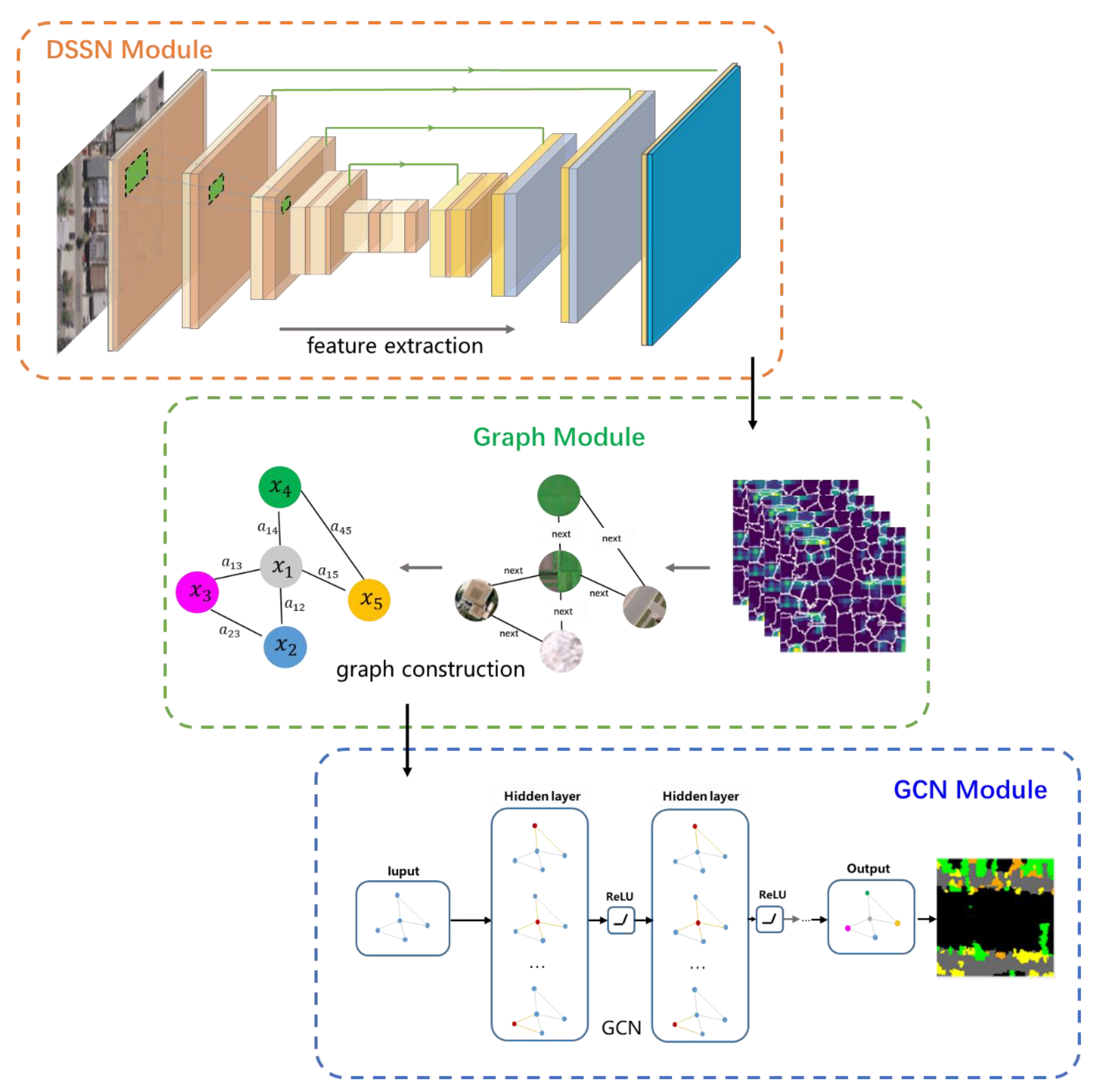
The workflow of the proposed DSSN-GCN framework is visually shown in Figure 1. In the graph module, in order to make full use of the object-level spatial relationship and reduce the impact of pixel-level random noise, objects (or superpixels) segmented by the superpixel segmentation algorithm represent graph nodes. Topological spatial relationships between the objects denote the connecting edges of the graph. In DSSN module, considering the powerful ability of feature extraction of DSSN, the DSSN is trained to extract the deep features to semantically initialize the intrinsic content of the graph nodes. In the GCN module, the GCN, which is good at modeling the irregular dependency relationship, converts the semantic segmentation task into the graph node classification task. With the help of the topological spatial relationships between objects and the deep features with strong generalization, the GCN models the relationships between graph nodes and classifies all nodes.

2.1. The Proposed DSSN: AttResUNet

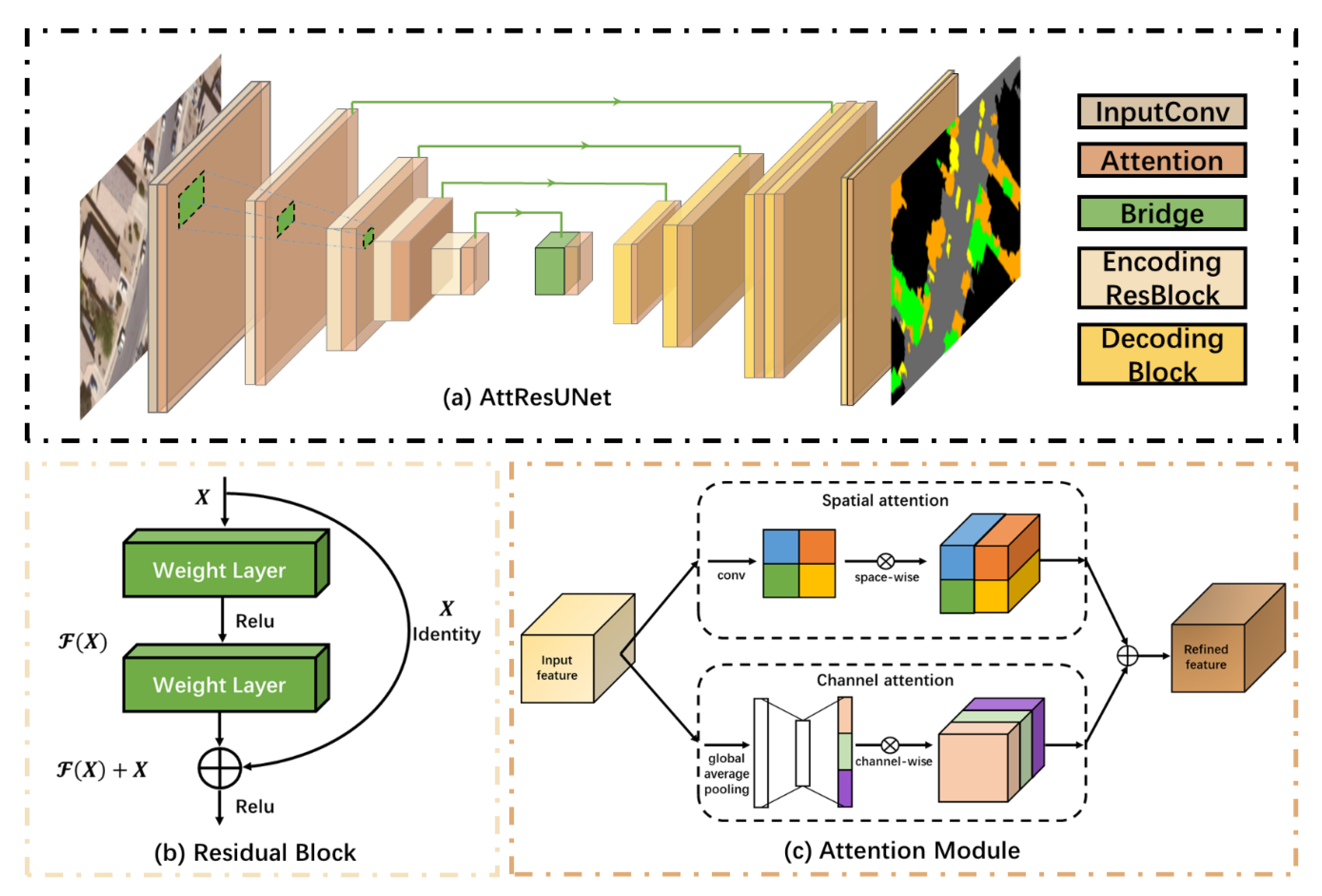
The proposed DSSN is shown in Figure 2. It consists of three parts: the U-shaped architecture with skip connections, the encoder based on residual blocks and the attention module, which is composed of spatial attention and channel attention in parallel. The attention module is placed after each block of AttResUNet to refine the extracted features.

In order to get a good result of semantic segmentation, it is very important to take low-level details into consideration, while retaining high-level semantic information. Especially for RS image, it contains richer detail information than natural images. The U-shaped architecture with skip connections strengthens the feature maps by combining low-level detail information from the encoder and high-level semantic information from the decoder, which allows DSSN to use these two kinds of information in segmentation. In general, the deeper network would get the better features. However, it could hamper the training because of gradient vanishing. He et al. [53] solved this problem by residual neural network (ResNet) that consists of a series of stacked residual blocks, as shown in Figure 2b, which allowed high-level gradients to be directly backpropagated through short connections to facilitate training to learn better features. The following formulas describe the residual block in detail.

$${\mathit{y}}_l=h\left({\mathit{x}}_l\right)+ℱ\left({\mathit{x}}_l,W_l\right)$$

(1)

$${\mathit{x}}_{l+1}=f\left({\mathit{y}}_l\right)$$

(2)

where ${\mathit{x}}_l$ and ${\mathit{x}}_{l+1}$ respectively represent the input and output of the $l$-th residual block. Each residual block generally contains a multilayer structure. $ℱ(·)$ is the residual function, which generates the residual by using layer weights $W_l$, the identity mapping function $h\left(·\right)$ is usually used as $\mathit{x}=h\left(\mathit{x}\right)$ and $f\left(·\right)$ is the rectified linear unit (ReLU) activation function.

In RS images, there are abundant ground objects and the extremely complex spatial distribution. It is important to automatically select regions of interest according to the task. In order to select and refine the features, the attention module with channel attention and spatial attention in [26] is applied to AttResUNet. Like the human visual system, the attention module can enhance meaningful features and suppress useless features, which is achieved by adjusting the weights of corresponding features. In the attention module shown in Figure 2c, spatial attention and channel attention are parallel. Features (C $\times$ H $\times$ W) from convolution layers are used as input. The spatial attention performs a 1 $\times$ 1 $\times$ 1 convolution and a sigmoid activation on the input feature to learn the spatial attention map (1 $\times$ H $\times$ W), which represents the importance of different spatial positions, then multiply the input with the spatial attention map to strengthen the expression of spatial semantic information. In the channel attention, the global average pooling is performed on the input feature at first. Then, there are two 1 $\times$ 1 $\times$1 convolution and a sigmoid activation to calculate the channel attention mask (C $\times$ 1 $\times$ 1). Finally, channel-wise multiplication is applied between the input feature and the mask to weight each channel according to its usefulness. At the end of the attention module, the outputs from spatial attention and channel attention are added together to fuse the channel information and the spatial information for semantic segmentation.

2.2. Feature Extraction Based on DSSN

In general, DSSN consists of an encoder and a decoder. The encoder extracts feature by convolutional layers and pooling layers. The decoder restores the feature maps to original image size with upsampling. After decoding, the results of segmentation are generated from input data.

$$p_c=\phi \cdot \varphi \left({\mathit{X}}_0,\theta \right), c=1,2,\dots ,n$$

(3)

$$\mathit{Y}=argmax\left(p_c\right)$$

(4)

where both input data ${\mathit{X}}_0\in {ℝ}^{w\times h\times channel}$ and output data $\mathit{Y}\in {ℝ}^{w\times h}$ have a width of $w$ and height of $h$. $\varphi$ is the encoder and $\phi$ is the decoder.

The probability of results belonging to class $c$ is $p_c$, and the total number of classes is n. In the back propagation, the neural network reduces the training loss by continuously adjusting the learnable parameters $\theta$ to optimize the results. The cross-entropy loss function $ℒ$ is often used for the semantic segmentation task, as the following:

$$ℒ=-{\displaystyle \sum }_{i=1}^w{\displaystyle \sum }_{j=1}^h{\displaystyle \sum }_{c=1}^n{y}_{ij}^{c}log\left(p_{ij}^c\right)$$

(5)

for pixel $\left(i,j\right)$, prediction from the forward propagation of network is $Y_{ij}\in \mathit{Y}$, if $Y_{ij}=c$, then $y_{ij}^c=1$, otherwise, $y_{ij}^c=0$.

After the supervised training, the DSSN has learned how to extract features that are effective to semantic segmentation. Obviously, features can be extracted from the encoder or decoder. Although the feature from the encoder is highly abstract, its size is small and details such as the spatial relationship are lost after convolution and pooling. The highly abstract feature is helpful to a one-hot task such as image classification, but is not suitable for semantic segmentation. On the contrary, the decoder recovers the original size of features and restores some details by upsampling. Therefore, we chose the features extracted by the decoder to initialize the graph.

2.3. Graph Construction

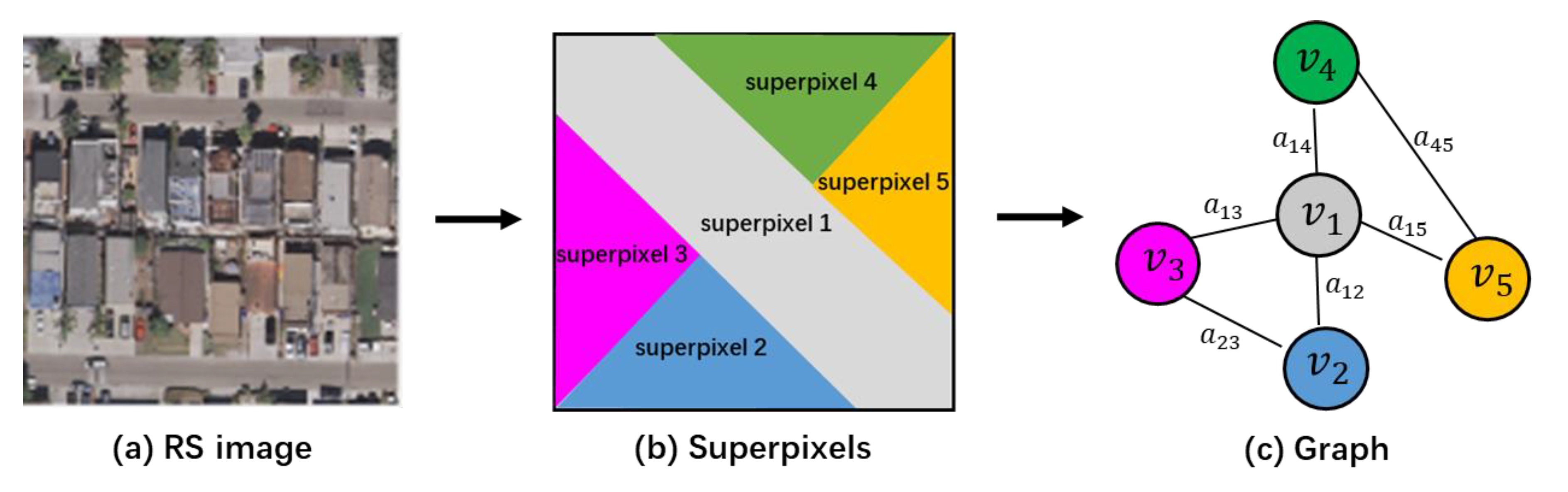
The objects and the relationships constitute an unstructured graph. The graph is represented by a tuple $Graph=\left(\mathit{V},\mathit{E}\right)$, where $\mathit{V}$ is the set of graph nodes and $\mathit{E}$ is the set of edges representing the connection between nodes. If $e_{ij}\in \mathit{E}$, node $v_i$ connects to node $v_j$ with edge $e_{ij}$. In the RS image, $\mathit{V}$ is a set of ground objects and $E$ represents the relationships between the objects. In order to construct the graph, as depicted in Figure 3, superpixels segmented by the unsupervised segmentation algorithm are used as graph nodes. Each superpixel is composed of a set of adjacent pixels with consistent characteristics. In addition, the first-order adjacency relationship (with common edge) between superpixels is regarded as graph edge to take the topological spatial relationship into consideration.

$$\mathit{V}=\left\{S_1,S_2,\dots ,S_k|S_i=Segment\left({\mathit{X}}_0\right),1\le i<K\right\}$$

(6)

where ${\mathit{X}}_0$ is the input image and $S_i$ denotes the i-th superpixel. $K$ is the total number of superpixels or nodes.

In the region of superpixel corresponding to node $v_i$, the average value of each channel of the deep features extracted by DSSN is taken as the node feature vector ${\mathit{x}}_i^G\in {\mathit{X}}^G$. The feature vector of the graph is ${\mathit{X}}^G={\left[{\mathit{x}}_1^G,{\mathit{x}}_2^G,\dots ,{\mathit{x}}_K^G\right]}^T\in {ℝ}^{K\times D}$, where $D$ is the dimension of the feature vector of the graph node.

For each node, we need to figure out which category it belongs to. It is easy to know the class of each pixel from the label image. In general, a homogeneous region, such as a superpixel, can be represented by its main characteristics, so it makes sense to specify the majority class as category for the region. Specifically, we counted the class of all pixels in each node and assigned the category that contains the maximum number of pixels with the same class as the label of the node.

The spatial adjacency relationships between the graph nodes are denoted by the adjacency matrix $\mathit{A}\in {ℝ}^{N\times N}$. Considering that the contributions of different nodes in the neighborhood to the central node are different, the strength of spatial relationship between them is determined by the spectral similarity and the spatial location. If node $v_i$ is adjacent to node $v_j$, the connecting edge between them has a weight $a_{ij}\in \mathit{A}$. To quantitatively express the strength of spatial relationship between $v_i$ and $v_j$, we set that the $a_{ij}$ is larger if the greater the spectral similarity between the two nodes.

$$\{\begin{array}{c}{a}_{ij}=0, \mathrm{if} v_i \mathrm{is} \mathrm{not} \mathrm{adjacent} \mathrm{to} v_j \\ a_{ij}=exp\left(-\frac{\parallel la{b}_i-la{b}_j\parallel }{{\sigma }_w^2}\right), \mathrm{if} v_i \mathrm{is} \mathrm{adjacent} \mathrm{to} v_j \end{array}$$

(7)

where $lab$ denotes the average color value of the node in the LAB color space of the Commission International Eclairage (CIELAB) and ${\sigma }_w^2$ controls the range of weight.

2.4. Node Classification via GCN

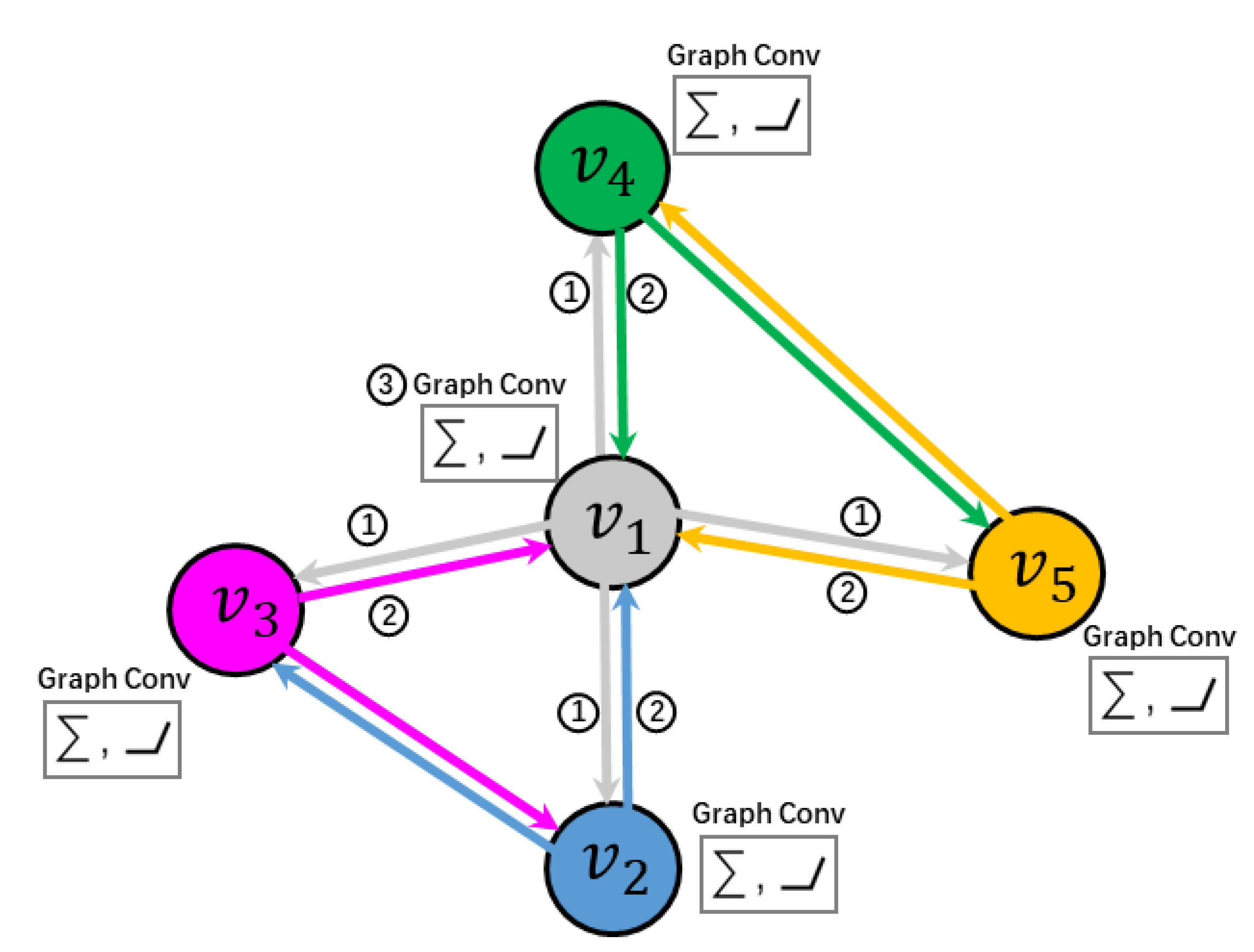
We adopted GCN, denoted as $g\left(\mathit{X},\mathit{A}\right)$, to get the classification $\mathit{Z}$ of the graph nodes. Same as CNN, GCN extracts features on graph structure data by convolution, which is called graph convolution. As shown in Figure 4, graph convolution consists of three steps. In the first step, each node sends its characteristic information to neighboring nodes. This step is to extract the characteristic information of the node. Every node collects the characteristic information from neighboring nodes and fuses the local structure and the characteristic information in the second step. In the third step, gather the previous information and then performs a nonlinear transformation to increase the expressive ability of the model.

Graph convolution aggregates the information of node from its neighbor nodes to generate a new representation. Therefore, using graph convolution on ground objects is useful for aggregating spatial information, which means that it is necessary to take matrix $\mathit{A}$ representing the relationships between nodes into consideration when calculating the features $\mathit{H}$ of each layer of GCN.

$$Z=g\left(\mathit{H},\mathit{A}\right)$$

(8)

$${\mathit{H}}^{\left(l+1\right)}=\sigma \left({\mathit{L}}_G{\mathit{H}}^{\left(l\right)}{\mathit{W}}^{\left(l\right)}\right),{\mathit{L}}_G={\tilde{\mathit{D}}}^{-\frac{1}{2}}\tilde{\mathit{A}}{\tilde{\mathit{D}}}^{-\frac{1}{2}}$$

(9)

where $H^{\left(l\right)}$ is the feature of layer $l$ of GCN, for the input layer ${\mathit{H}}^{\left(0\right)}={\mathit{X}}^G$. $\sigma$, $\mathit{W}$ and ${\mathit{L}}_G$ are the nonlinear activation function, the learnable parameter matrix and the Laplacian matrix respectively. $\tilde{\mathit{A}}=\mathit{A}+\mathit{I}$, where $\mathit{I}$ is the identity matrix. $\tilde{\mathit{D}}$ is the degree matrix of $\tilde{\mathit{A}}$.

In the training process, GCN adjusts $\mathit{W}$ by continuously reducing loss, thereby optimizing the output, as shown:

$$ℒ={\displaystyle \sum }_{i=1}^{n}loss\left(g\left({\mathit{X}}_i^G,\mathit{A}\right),T_i\right)$$

(10)

where $T_i$ is the ground truth of training sample $i$ and the number of samples is $n$. $ℒ$ is the loss function, such as the cross entropy loss function.

When finishing training, the GCN combines features ${\mathit{X}}^G$ and adjacent matrix $\mathit{A}$ to classify the graph nodes. As the nodes are from superpixels, each node corresponds to a region on the image. The class of all pixels in the region is the same as the category of the corresponding node, thereby the entire semantic segmentation of the image is completed.

In general, the process of our DSSN-GCN framework is composed of three steps above including feature extraction based on DSSN, graph construction and node classification via GCN, which is in brief captured in Algorithm 1.

Algorithm 1. Combining DSSN and GCN for Semantic Segmentation of Remote Sensing Imagery

Input: the remote sensing image dataset ${\mathit{D}}_T$; the number of superpixels $k$. 1. Train DSSN with samples from ${\mathit{D}}_T$. 2. Use the DSSN to extract high-level features ${\mathit{X}}_f=\left\{x_1,x_2,\dots ,x_D\right\}$. 3. Construct the graph nodes $\mathit{V}$. Regions segmented by the unsupervised segmentation algorithm are used as graph nodes $\mathit{V}=\left\{v_1,v_2,\dots ,v_k\right\}$. Use features ${\mathit{X}}_f$ to semantically initialize the intrinsic content of the graph nodes, represented as ${\mathit{X}}^G={\left[{\mathit{x}}_1^G,{\mathit{x}}_2^G,\dots ,{\mathit{x}}_K^G\right]}^T\in {ℝ}^{K\times D}$. 4. Construct the graph edges $\mathit{E}$. Take the first-order adjacency relationships (with common edge) between the graph nodes as the graph edges and calculate the strength of the edges. 5. After the training of the GCN, adopt the GCN to perform classification on the graph nodes. 6. Get the maps of semantic segmentation. Assign the category of each node to the pixels located in the node. Output: the maps of semantic segmentation.

3. Experiments

In this section, the data description and details of experimental settings were introduced at first. The experimental results and analysis were given after that.

3.1. Datasets and Evaluation Metrics

To test our method, experiments were performed on the UCM dataset [54] and the DeepGlobe dataset [56].

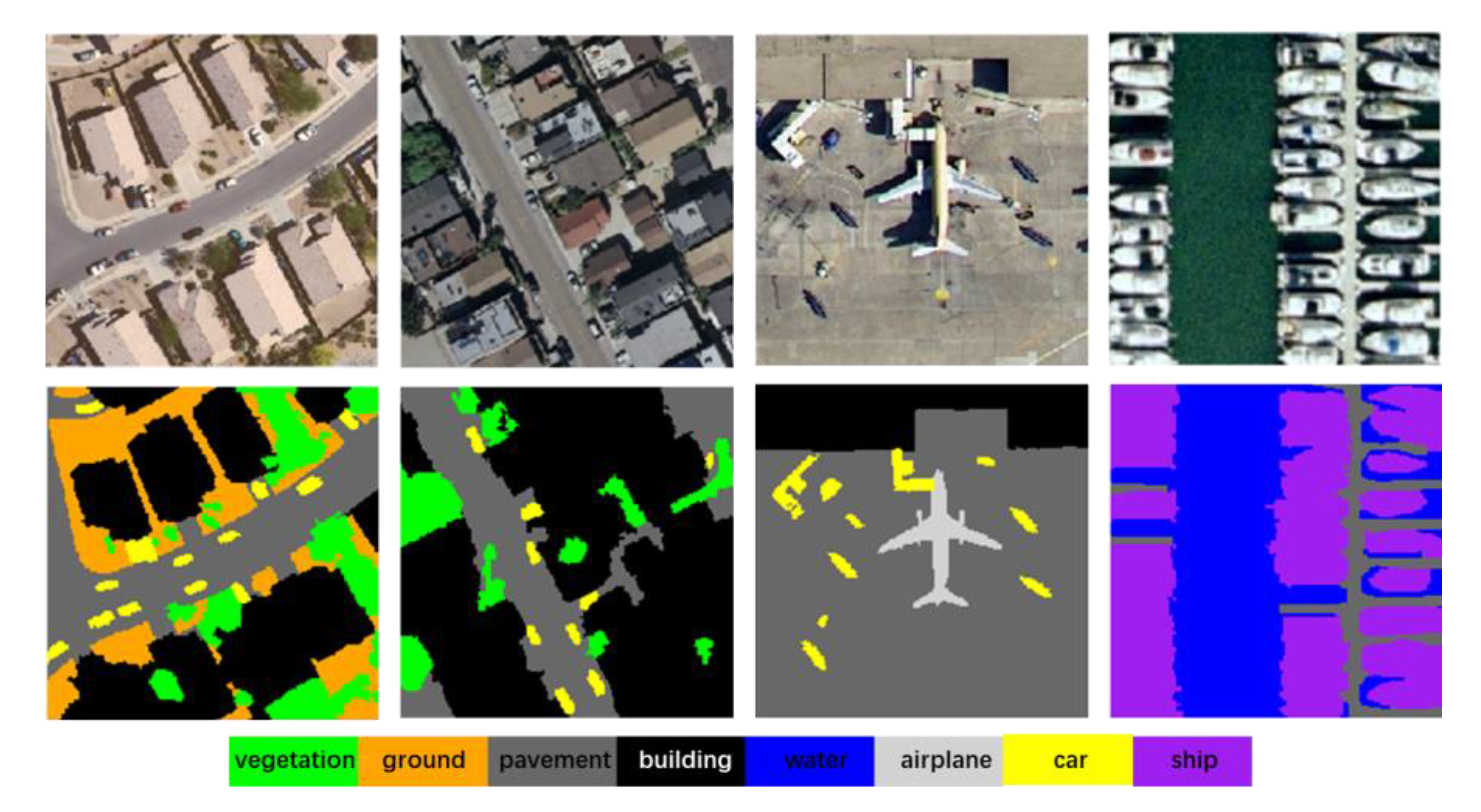
As visually illustrated in Figure 5, the UCM dataset that contains 2100 aerial images with 0.3 m spatial resolution and 256 × 256-pixel size was labeled into 17 categories for semantic segmentation on DLRSD dataset [54]. In order to reduce the similarity between the classes [43], we merged the 17 classes into 8 classes, which are vegetation (trees and grass), ground (bare soil, sand and chaparral), pavement (pavement and dock), building (building, mobile home and tank), water (water and sea), airplane (airplane), car (car) and ship (ship), and removes images containing a field or tennis court. Each category is a combination of the original categories in the parentheses. These filtered images are randomly divided into the training set, validation set and test set, each with 1513, 189 and 190 images, with the proportions of 80%, 10% and 10% respectively. The class distribution for UCM dataset can be seen in

Table 1. The class distribution for the UCM dataset (%).

UCM	Vegetation	Pavement	Ground	Building	Water	Car	Ship	Airplane
all	28.59	27.38	17.63	13.65	7.87	2.88	1.62	0.36
train	29.23	27.17	17.37	13.58	7.84	2.84	1.61	0.35
validation	25.65	30.62	16.71	13.38	8.61	2.63	1.80	0.60
test	26.43	25.77	20.66	14.51	7.39	3.47	1.55	0.21

. The four categories of vegetation, pavement, ground and building account for the first, the second, the third and the fourth place respectively. The proportion of top four categories was more than 85% and the proportion of airplane was the least (less than 0.5%).

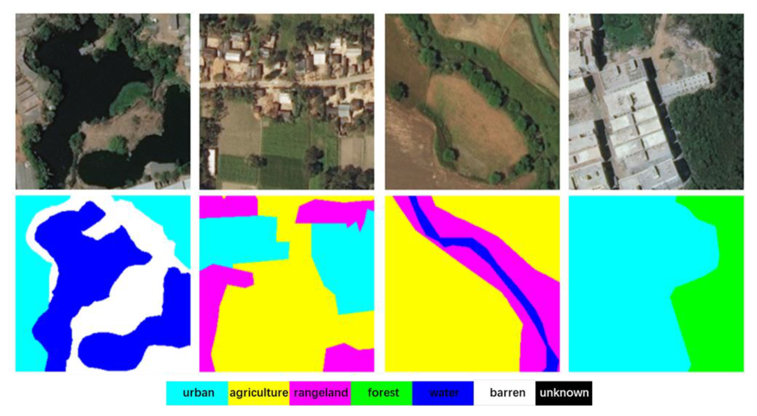
The DeepGlobe dataset [55], as shown in Figure 6 provides 1146 submeter high-resolution images with a size of 2448 × 2448. Seven categories are manually labeled, namely urban, agriculture, rangeland, forest, water, barren and unknown. As shown in

Table 2. The class distribution for the DeepGlobe dataset (%).

DeepGlobe	Agriculture	Urban	Forest	Rangeland	Barren	Water	Unknown
all	57.88	10.80	11.11	8.41	8.43	3.33	0.05
train	58.42	10.93	9.98	8.51	8.80	3.31	0.06
validation	56.16	7.50	19.27	7.78	5.04	4.23	0.01
test	55.29	13.05	11.99	8.26	8.82	2.59	0.01

, there is a large imbalance in the dataset that the area of agriculture is more than 50% and the share of urban and forest are 10.93% and 9.98% respectively. Moreover, the proportion of unknown is close to 0% meaning few pixels of unknown in the ground truth masks. The entire dataset was divided into the training set, validation set and test set, containing 803, 171 and 172 images respectively. Images with a size of 256 × 256 are uniformly cropped from every raw image. These cropped images were randomly divided into the training set, validation set and test set, each with 10,272, 1280 and 1296 images, with the proportions of 80%, 10% and 10% respectively.

In this paper, the overall accuracy (OA), the intersection over union (IoU) and the frequency weighted intersection over union (FWIoU) are adopted as the evaluation metrics [58].

$$OA=\left(TP+TN\right)/\left(TP+FP+TN+FN\right)$$

(11)

$$Io{U}_i=\frac{T{P}_i}{T{P}_i+F{P}_i+F{N}_i} , i=1,2,\dots ,n$$

(12)

$$FWIoU={\displaystyle \sum }_1^n\left(Io{U}_i·\frac{T{P}_i+F{N}_i}{T{P}_i+F{P}_i+T{N}_i+F{N}_i}\right)$$

(13)

where $TP$, $TN$, $FP$ and $FN$ are the number of true positive points, true negative points, false positive points and false negative points respectively. $n$ is the number of classes.

3.2. Implementation Details

In this paper, we used three representative backbones and a proposed network as DSSN for feature extraction: U-Net [19], SegNet [20], DeepLab V3+ [25] and the proposed AttResUNet. On this basis, four neural networks are proposed: DSSN-GCN V1 with U-Net, DSSN-GCN V2 with SegNet, DSSN-GCN V3 with DeepLab V3+ and DSSN-GCN V4 with AttResUNet. For U-Net and SegNet, they are widely used as the baseline model for RS image semantic segmentation. The DeepLab V3+ network is a new method, which has achieved the state-of-the-art semantic segmentation results on the natural image. The network structure of AttResUNet is shown in

Table 3. The network structure of AttResUNet.

	Layers	Ouput Size
Input	input	H $\times$ W $\times$ 3
InputConv	conv 7 $\times$ 7, stride 2	H/2 $\times$ W/2 $\times$ 64
	attention module	H/2 $\times$ W/2 $\times$ 64
	maxpool 3 $\times$ 3, stride 2	H/4 $\times$ W/4 $\times$ 64
Encoder1	ResBlock1	H/4 $\times$ W/4 $\times$ 256
	attention module	H/4 $\times$ W/4 $\times$ 256
Encoder2	ResBlock2	H/8 $\times$ W/8 $\times$ 512
	attention module	H/8 $\times$ W/8 $\times$ 512
Encoder3	ResBlock3	H/16 $\times$ W/16 $\times$ 1024
	attention module	H/16 $\times$ W/16 $\times$ 1024
Encoder4	ResBlock4	H/32 $\times$ W/32 $\times$ 2048
	attention module	H/32 $\times$ W/32 $\times$ 2048
Bridge	conv 3 $\times$ 3, stride 1	H/32 $\times$ W/32 $\times$ 192
	attention module	H/32 $\times$ W/32 $\times$ 192
Decoder1	deconv 4 $\times$ 4, stride 2	H/16 $\times$ W/16 $\times$ 128
	concatenation	H/16 $\times$ W/16 $\times$ (1024 + 128)
	conv 3 $\times$ 3, stride 1	H/16 $\times$ W/16 $\times$ 128
	attention module	H/16 $\times$ W/16 $\times$ 128
Decoder2	deconv 4 $\times$ 4, stride 2	H/8 $\times$ W/8 $\times$ 96
	concatenation	H/8 $\times$ W/8 $\times$ (512 + 96)
	conv 3$\times$3, stride 1	H/8 $\times$ W/8 $\times$ 96
	attention module	H/8 $\times$ W/8 $\times$ 96
Decoder3	deconv 4 $\times$ 4, stride 2	H/4 $\times$ W/4 $\times$ 64
	concatenation	H/4 $\times$ W/4 $\times$ (256 + 64)
	conv 3 $\times$ 3, stride 1	H/4 $\times$ W/4 $\times$ 64
	attention module	H/4 $\times$ W/4 $\times$ 64
Decoder4	deconv 4$\times$4, stride 2	H/2 $\times$ W/2 $\times$ 48
	conv 3 $\times$ 3, stride 1	H/2 $\times$ W/2 $\times$ 48
	attention module	H/2 $\times$ W/2 $\times$ 48
Decoder5	deconv 4 $\times$ 4, stride 2	H $\times$ W $\times$ 32
	conv 3 $\times$ 3, stride 1	H $\times$ W $\times$ 32
	conv 1 $\times$ 1, stride 1	H $\times$ W $\times$ C
	attention module	H $\times$ W $\times$ C
Output	output	H $\times$ W

. We adopted the residual block1-4 from ResNet-101 [53] pretrained on ImageNet dataset as the encoder. The decoder uses 3 $\times$ 3 convolutions and 4$\times$4 transposed convolutions to recover the original input size. For the training of DSSN, the stochastic gradient descent method (SGD) and the cross entropy were adopted as the optimizer and the loss function respectively.

The simple linear iterative cluster (SLIC) [59] was used to segment images to get the ground objects (or superpixels). Features of each object were from the mean values of the feature maps of the upsampling layer within the corresponding region of the object. We adopted the feature maps from layers of the DSSN networks above: feature map for DSSN-GCN V1, DSSN-GCN V2, DSSN-GCN V3 and DSSN-GCN V4 were all obtained from the last layer of its DSSN. To initialize the graph, the features of the objects were used as the features of the graph nodes in GCN [47]. The SGD optimizer and the cross-entropy loss function were used for the training of the GCN. With these settings, extensive experiments including sensitivity analysis were performed to choose the best critical parameters and examine the effectiveness of the proposed DSSN-GCN model. All the experiments were conducted on the Pytorch framework with NVIDIA 1080Ti GPU.

3.3. Sensitivity Analysis of Critical Parameters

Hyperparameters in our proposed method mainly included the number of superpixels $k$, the similarity factor ${\sigma }_w^2$ and the number of GCN layers $l$. $k$ determines the number of ground objects (or superpixels) in the graph. ${\sigma }_w^2$ controls the range of value of adjacent matrix in the graph. $l$ is the number of layers of GCN, which represents the depth of the network.

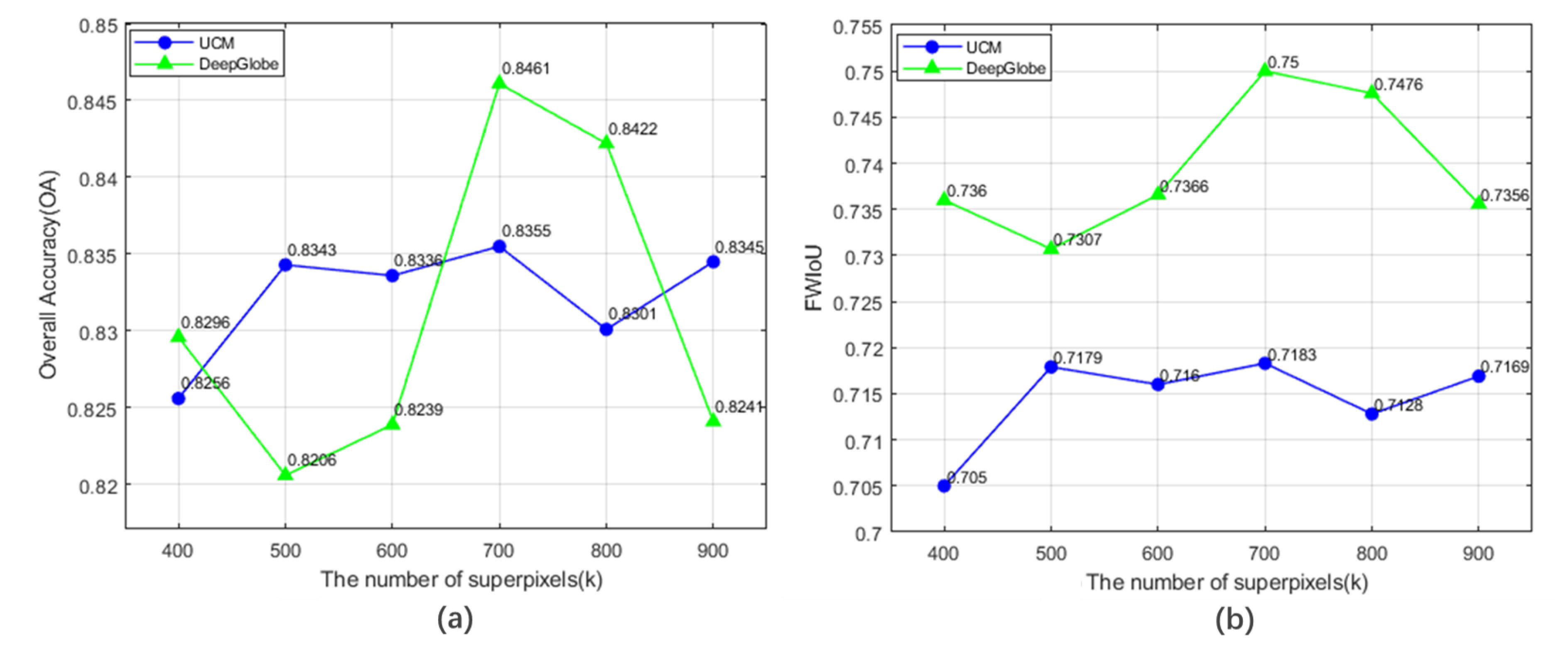
As the representation of the ground object on the image, the superpixel, which retains the boundary of the ground object, is composed of a set of pixels with similar characteristics such as color, brightness, texture, etc. Therefore, converting the pixel-by-pixel classification to the object-based node classification can not only reduce the time consumption of classification, but also reduce noises and restore the boundary of the ground objects to a certain degree. The number of superpixels in an image determines the size of each superpixel. The smaller $k$, the larger the area corresponding to one superpixel. If the superpixel is too small, the characteristic information will be insufficient, on the contrary, details would be lost. In (a) and (b) of Figure 7, it shows that the best $k$ for the UCM dataset and the DeepGlobe dataset were both 700 respectively.

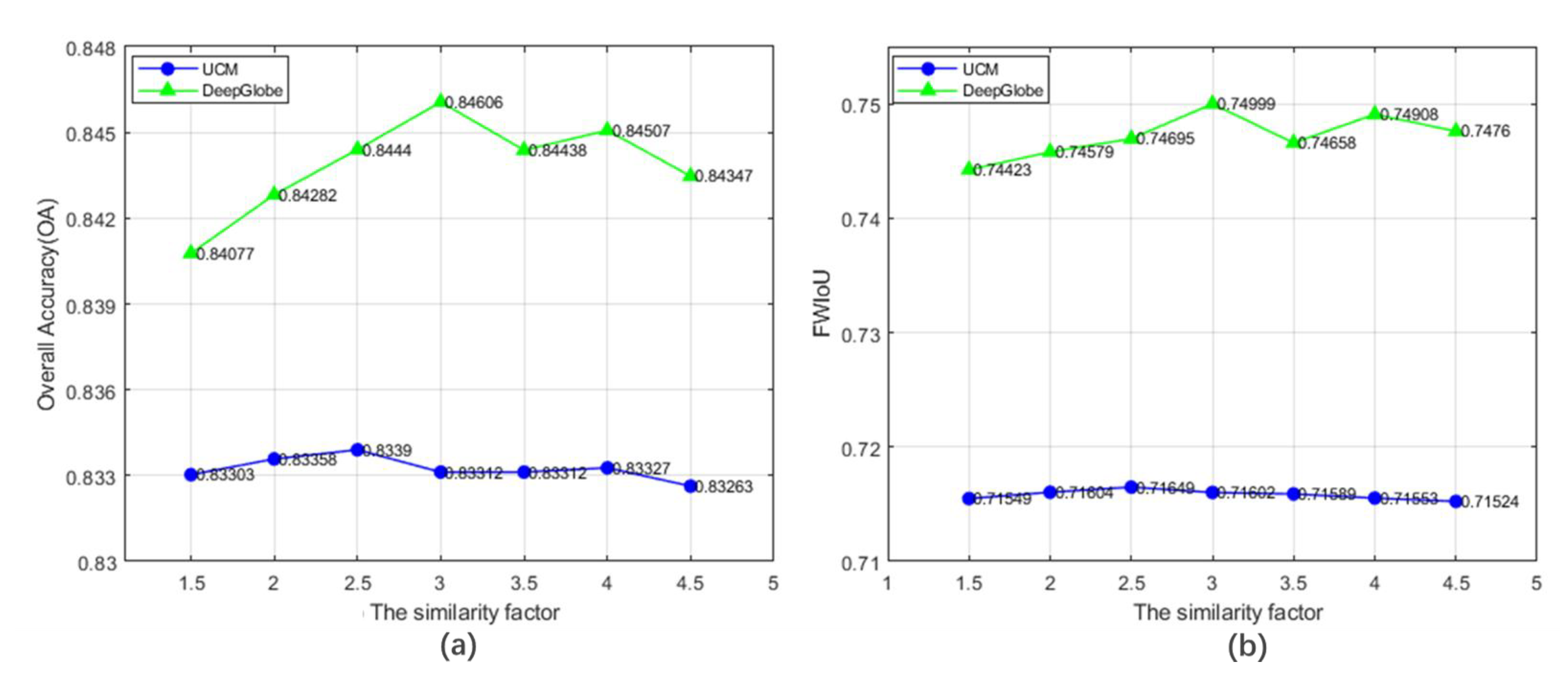
The adjacency matrix in the graph depicts the spatial relationship between nodes. The matrix values reflect the strength of the relationship and its distribution is controlled by the similarity factor ${\sigma }_w^2$. (a) and (b) of Figure 8 illustrate the accuracy of segmentation in different ${\sigma }_w$. With the increase of the similarity factor, both OA and FWIoU rose at first and then decreased. When ${\sigma }_w^2=2$ on the UCM dataset and ${\sigma }_w^2=3$ on the DeepGlobe dataset, the best performance was obtained.

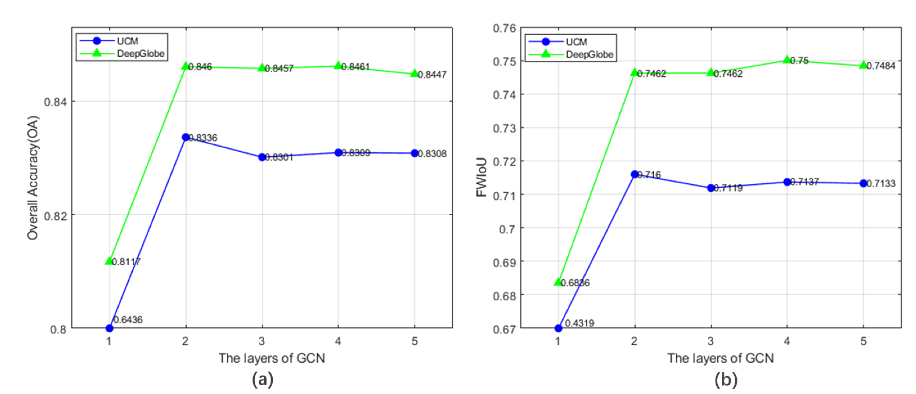
The number of layers was positively correlated with the complexity of the neural network. In general, the deeper the model structure, the better the fitting effect. However, due to the gradient vanishing, GCN was usually limited to shallow layers ($l=2–4$) [50]. In view of this problem, we tested our DSSN-GCN model with 1–5 layers of GCN. In Figure 9a,b, as the layers of GCN increased, OA and FWIoU both increased up to the maximum. The accuracy of segmentation reached the best value when $l=2$ on the UCM dataset and when $l=4$ on the DeepGlobe dataset. Additionally, it is worth noting that OA and FWIoU were both poor when GCN had only one layer, because the layer of GCN was too shallow to learn better feature expression.

3.4. Comparison with the State-of-the-Art Method

In order to evaluate the performance of our proposed DSSN-GCN model, experiments were conducted on the UCM dataset and the DeepGlobe dataset. In the experiments, we tested four DSSN-GCN networks, which were DSSN-GCN V1 based on U-Net, DSSN-GCN V2 based on SegNet, DSSN-GCN V3 based on DeepLab v3+ and DSSN-GCN V4 based on the proposed AttResUNet, respectively.

3.4.1. Results on the UCM Dataset

The overall accuracy of semantic segmentation on the UCM dataset is shown in the last column of

Table 4. The overall accuracy (OA) (%) of semantic segmentation on the UCM dataset.

Model	Vegetation	Ground	Pavement	Building	Water	Car	Ship	Airplane	Overall (OA)
U-Net	81.21	73.13	90.03	65.10	89.58	72.61	87.52	0	79.72
DSSN-GCN v1	84.22	80.76	85.69	71.85	89.16	69.79	80.25	0	81.71
SegNet	81.35	77.34	83.31	75.97	87.94	70.74	85.45	10.00	80.28
DSSN-GCN v2	83.44	76.52	84.18	80.01	88.16	63.99	82.02	0	81.17
DeepLab v3+	80.13	77.85	80.97	86.05	87.07	75.63	93.73	57.27	81.25
DSSN-GCN v3	82.30	78.87	85.45	80.78	86.18	68.35	91.02	0	81.94
AttResUNet	85.77	75.62	86.44	86.76	92.30	82.04	87.60	58.43	84.31
DSSN-GCN V4	86.67	77.06	88.08	86.80	93.57	75.72	81.29	33.78	85.00

and

Table 5. The intersection over union (IoU) (%) of semantic segmentation on the UCM dataset.

Model	Vegetation	Ground	Pavement	Building	Water	Car	Ship	Airplane	Overall (FWIoU)
U-Net	70.20	61.14	68.71	56.73	79.65	62.02	68.45	0	66.23
DSSN-GCN v1	71.33	64.03	73.08	62.80	81.32	59.65	68.29	0	69.17
SegNet	68.47	65.14	69.16	60.31	80.60	59.82	63.95	9.62	67.18
DSSN-GCN v2	69.32	66.17	70.77	62.53	81.84	58.45	66.05	0	68.41
DeepLab v3+	68.34	65.17	71.77	65.54	81.93	61.54	58.14	37.62	68.71
DSSN-GCN v3	69.33	65.64	72.87	67.21	82.25	61.25	59.67	0	69.55
AttResUNet	72.42	65.72	77.11	71.02	86.01	70.67	76.09	49.53	72.99
DSSN-GCN V4	73.47	67.03	77.87	73.24	87.36	68.18	72.87	33.07	73.99

. The OA/ FWIoU increased by 1.99%/2.94% for DSSN-GCN V1 compared to the U-Net, the OA/FWIoU rose by 0.89%/1.23% for DSSN-GCN V2 compared to the SegNet, the OA/FWIoU increased by 0.68%/0.84% for DSSN-GCN V3 compared to the DeepLab V3+ and DSSN-GCN V4 improved the OA/FWIoU by 0.69%/1%. Each DSSN-GCN outperformed its DSSN, which proved the effectiveness of the integration of DSSN and GCN in DSSN-GCN framework. Moreover, Table 4 and Table 5 shows that the proposed AttResUNet was better than all reference methods and DSSN-GCN V4 achieved the best semantic segmentation results, which demonstrated the advance of our AttResUNet.

Table 4 and Table 5 reported respectively the OA and the IoU of semantic segmentation of each category on the UCM dataset. Due to the class imbalance, the main categories including vegetation, ground, pavement and building were more than 85% (Table 1) in the dataset. Considering the top four categories, it can be seen that DSSN-GCN V1 improved the OA/IoU of vegetation, ground and building by 3.01%/1.13%, 7.63%/2.89% and 6.75%/6.07% respectively compared with the U-Net, DSSN-GCN V2 rose the OA/IoU of vegetation, pavement and building by 2.09%/0.85%, 0.87%/1.16% and 4.04%/2.22% respectively on the basis of the SegNet and DSSN-GCN V3 achieved an improvement in the OA/IoU of vegetation, ground and pavement by 2.17%/0.99%, 1.02%/0.47% and 4.48%/1.1% respectively compared to DeepLab v3+, and DSSN-GCN V4 improved the OA/IoU of the main categories by 0.9%/1.05%, 1.44%/1.31%, 1.64%/0.76% and 0.04%/2.22% respectively. As shown in Table 5, the IoUs of the top five classes (top four categories and water) of our proposed DSSN-GCN models (including V1, V2, V3 and V4) were higher than that of backbones (including U-Net, SegNet, DeepLab V3+ and AttResUNet) by 1–6%. However, the IoUs of airplane exceeded that of DSSN-GCN models. Though the airplane made up a quite low share (0.36%) of the UCM dataset, the IoU of airplane still contributed 1/8 (eight categories in the UCM dataset) to the MIoU. Therefore, it is reasonable to adopt the FWIoU metric to evaluate semantic segmentation methods under the circumstance of the class imbalance.

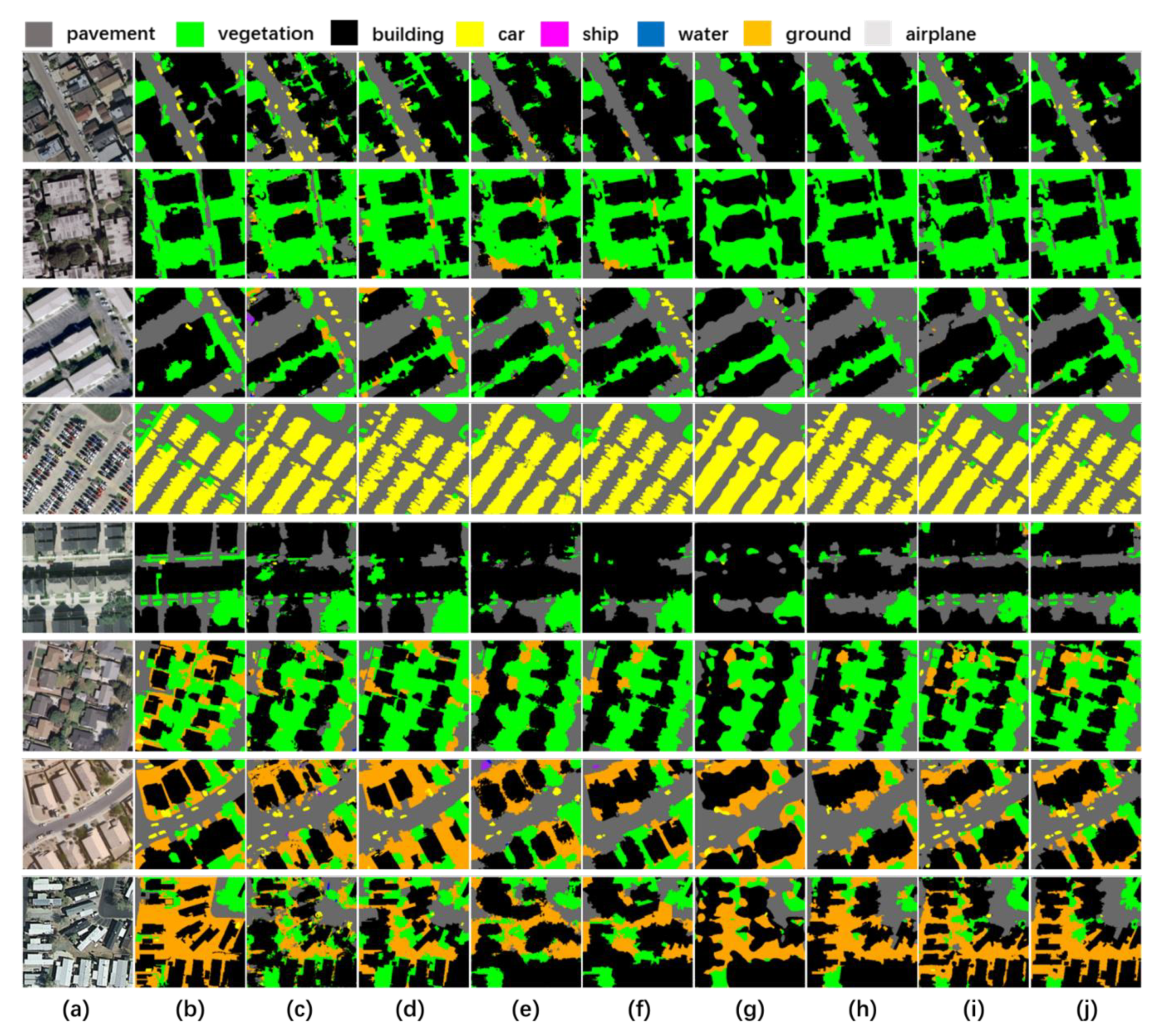
To compare results of all models above, we visualized the results of the proposed DSSN-GCN models and other referenced methods. In Figure 10, we could see the results of U-Net, DSSN-GCN V1, SegNet, DSSN-GCN V2, DeepLab V3+, DSSN-GCN V3, the proposed AttResUNet and AttResUNet-GCN (DSSN-GCN V4) from (c) to (j). It presents that segmentation of our DSSN-GCN model was more accurate and consistent compared to its backbone network, shown in (d) to (c), (f) to (e), (h) to (g) and (j) to (i), which explained the effectiveness of the proposed DSSN-GCN model to improve the results of semantic segmentation. AttResUNet-GCN with the best FWIoU (73.99%) achieved the best results and results of AttResUNet were better than that of other backbones, which demonstrated the advance of the proposed AttResUNet. In addition, the results of DSSN-GCN models were less noisy and possessed more accurate boundaries, especially in building, car and pavement.

3.4.2. Results on the DeepGlobe Dataset

The last column of

Table 6. The OA (%) of semantic segmentation on the DeepGlobe dataset.

Model	Urban	Agriculture	Rangeland	Forest	Water	Barren	Unknown	Overall (OA)
U-Net	71.67	87.03	47.06	90.65	73.74	63.96	0	79.77
DSSN-GCN v1	85.43	88.87	50.53	87.91	75.38	55.64	0	81.86
SegNet	82.68	90.00	52.33	84.65	73.16	57.37	0	81.97
DSSN-GCN v2	83.79	91.95	46.30	85.42	74.52	53.76	0	82.51
DeepLab v3+	88.67	89.21	55.39	90.09	77.48	70.18	0	84.46
DSSN-GCN v3	86.63	92.03	55.66	86.81	76.12	66.98	0	85.07
AttResUNet	84.56	91.37	56.35	89.64	81.71	75.16	0	85.70
DSSN-GCN V4	84.60	91.16	56.61	89.95	82.09	76.90	0	85.81

and

Table 7. The IoU (%) of semantic segmentation on the DeepGlobe dataset.

Model	Urban	Agriculture	Rangeland	Forest	Water	Barren	Unknown	Overall (FWIoU)
U-Net	65.61	80.65	28.02	69.39	59.08	41.67	0	68.99
DSSN-GCN v1	72.72	81.91	29.49	74.16	59.41	43.94	0	71.52
SegNet	72.57	81.76	29.89	75.53	61.64	44.66	0	71.74
DSSN-GCN v2	73.34	82.15	28.74	75.94	62.69	43.86	0	71.96
DeepLab v3+	74.53	83.23	37.66	79.52	60.89	52.82	0	74.62
DSSN-GCN v3	75.58	84.17	37.92	79.40	61.67	53.28	0	75.35
AttResUNet	75.32	84.71	38.69	79.18	69.53	58.34	0	76.30
DSSN-GCN V4	75.60	84.77	39.09	79.29	69.48	58.95	0	76.47

shows the overall accuracy of semantic segmentation on the DeepGlobe dataset. It shows the advance of our proposed DSSN that AttResUNet achieved the best performance compared to other DSSNs. The OA/FWIoU increased by 2.09%/2.53% for DSSN-GCN V1 compared to the U-Net. DSSN-GCN V2 rose the OA/FWIoU by 0.54%/0.22% compared with the SegNet. DSSN-GCN V3 achieved improvement in the OA/FWIoU by 0.61%/0.73% on the basis of DeepLab V3+. Compared with AttResUNet, DSSN-GCN V4 improved the OA/IoU by 0.11%/0.17%. The OA/FWIoU of DSSN-GCN model were better than that of its backbone and the best OA/FWIoU were 85.81%/76.30% from DSSN-GCN V4, which demonstrated the effectiveness of the DSSN-GCN model.

The OA and the IoU of semantic segmentation of each category on the DeepGlobe dataset are presented in Table 6 and Table 7, respectively. There was a large class imbalance in the dataset that main categories including agriculture (58%), urban (11%) and forest (11%) were more than 80% (Table 2). Considering the top three categories, it could be seen that DSSN-GCNs had advantages in OA compared to the corresponding DSSNs. Furthermore, the IoUs of top four categories of DSSN-GCN were almost better than its backbone. In addition, DSSN-GCN V1 increased in IoU of all categories, especially 13.76%/7.11% improvement in the OA/IoU of urban. However, in the next to last column of Table 6 and Table 7, all the OA/IoU of unknown were 0. This is because that the proportion of unknown in the dataset (counting for 0.05%) was too low to be learned and recognized by the classifier.

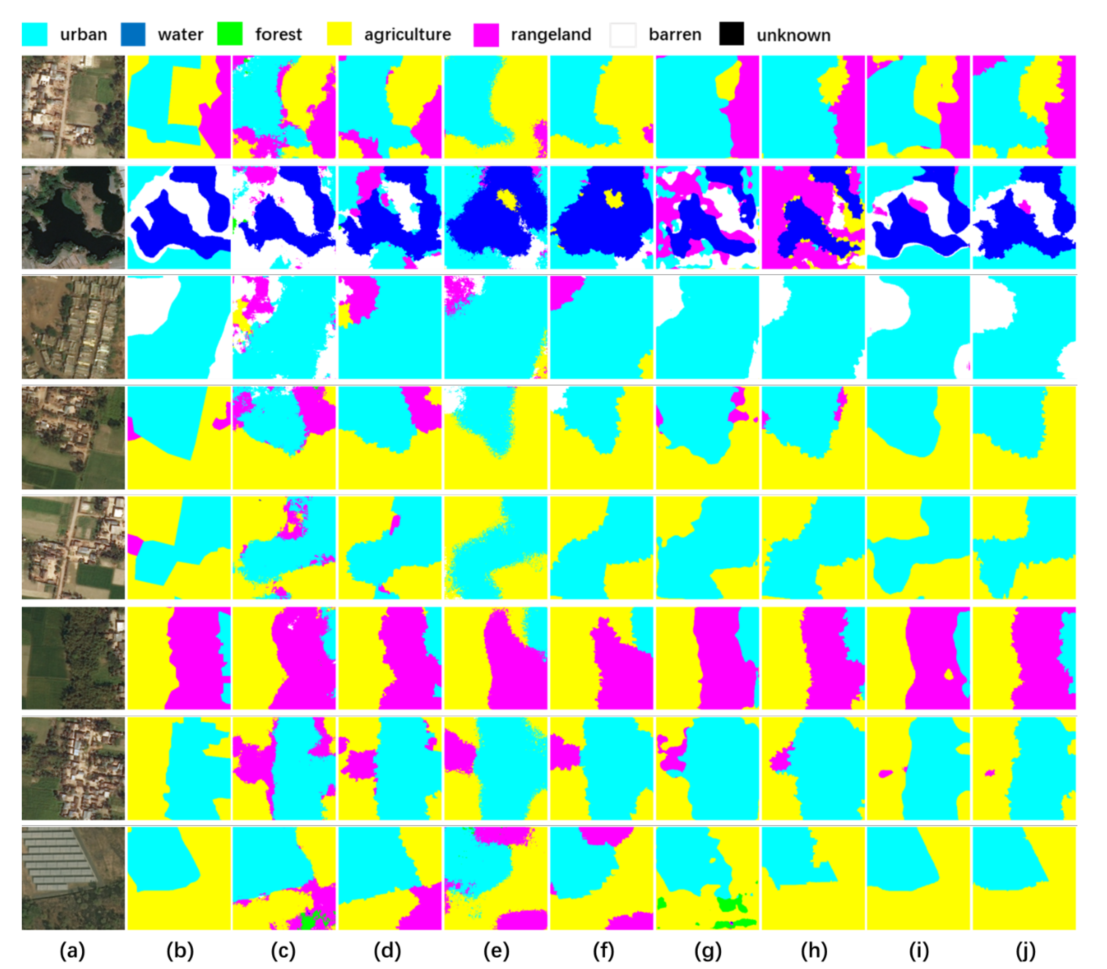
The visible semantic segmentation of the DeepGlobe dataset was presented to qualitatively verify the conclusions of the paragraph above. It can be seen in Figure 11 that the results from (c) to (j) were the segmentation maps of the results of U-Net, DSSN-GCN V1, SegNet, DSSN-GCN V2, DeepLab V3+, DSSN-GCN V3, the proposed AttResUNet and AttResUNet-GCN (DSSN-GCN V4). It shows that our DSSN-GCN models achieved more accurate and consistent segmentation compared to its backbone network, shown in (d) to (c), (f) to (e), (h) to (g) and (j) to (i), which demonstrated that the proposed DSSN-GCN model was effective to improve the results of semantic segmentation. Moreover, the proposed AttResUNet achieved better results than other backbones and AttResUNet-GCN with the best OA and FWIoU on this dataset got the best result.

4. Discussion

In this paper, we analyzed the sensitivity of critical parameters including the number of superpixels $k$, the similarity factor ${\sigma }_w^2$ and the number of GCN layers $l,$ which have an important influence on the proposed DSSN-GCN model. In the model, $k$ determines the size and number of graph nodes, the value range of the strength of the spatial relationship was controlled by ${\sigma }_w^2$, and $l$ reflects the expression ability of GCN. In order to build the graph in GCN, we constructed graph nodes through the superpixel segmentation and transformed pixel-level segmentation into node classification. The number of superpixels should be selected carefully. Since if the superpixel is too small, the characterization information will be insufficient, on the contrary, details would be lost. According to the experimental results, the best $k$ of our model for the UCM dataset and the DeepGlobe dataset were both 700. However, it is urgent to improve the speed and the accuracy of the methods for node construction. In the graph, the relationships between nodes were also of importance, which constitute the path of information transmission in GCN. When constructing the connection edges between nodes, we comprehensively considered the spatial relationship (the first-order adjacency relationship) and the spectral information (values in the CIE LAB color space) to quantify the strength of spatial relationships, and adopt the similarity factor ${\sigma }_w^2$ to control the value range of these edges. By doing that, the strength of spatial relationship between different nodes is of difference. Moreover, the number of layers is the key parameter of the neural network. Due to the problem of gradient vanishing, GCNs are limited to shallow layers. Although there are some works to construct deep GCNs [50], the classification accuracy still needs further improvement. In view of this problem, we tested the proposed DSSN-GCN model with 1–5 layer GCN and got the best performance on the UCM dataset for $l=2$ and on the DeepGlobe dataset for $l=4$.

In order to verify the effectiveness of our model, we designed four DSSN-GCN models based on different backbones including the proposed AttResUNet, the classic U-Net model, SegNet and DeepLab V3+, which is the state-of-the-art model in natural image semantic segmentation. The DSSN-GCN models (V1, V2, V3 and V4) and the contrast methods were applied to the experiments. We chose the metrics of OA and FWIoU to measure the results of semantic segmentation. Additionally, the FWIoU metric was adopted because it was widely used in semantic segmentation and more reasonable than MIoU under the circumstance of the class imbalance. The segmentation results on two datasets in Table 4,Table 5,Table 6 and Table 7 present that the DSSN-GCN model outperformed its backbone and DSSN-GCN V4 achieved the best performance both on the two datasets, which proved the effectiveness of our DSSN-GCN model. Meanwhile, it shows the importance of the spatial relationship for high-precision semantic segmentation and the relationship modeling ability of GCN. Moreover, there is a large improvement of the proposed AttResUNet compared to other advanced DSSNs, which shows the advance of our AttResUNet. The OA/IoU of AttResUNet for the small objects, such as car, ship and airplane in the UCM dataset, are increased significantly compared to U-Net. However, the performance of DSSN-GCN V4 on small objects such as car, ship and airplane is inferior to the proposed AttResUNet. This is because with the help of the residual blocks-based encoder and the attention model, AttResUNet can extract deep features with stronger expression and select regions of interest automatically, which is helpful for the segmentation of small objects. In addition, there were few samples for the training of GCN and some detailed information will be lost in object-level modeling of DSSN-GCN, which would bring a negative impact on the recognition of small objects. From Table 1 and Table 2, the samples of airplane count for only 0.36% on the UCM dataset, which was the same as the unknown (0.05%) on the DeepGlobe dataset. These samples were too few to train DSSN to learn expression of the airplane, which caused all the OA and the IoU of the airplane to be quite low in Table 4 and Table 5 and even all the OA and the IoU of the unknown to be 0% in Table 6 and Table 7. This phenomenon reflected that DSSN model was not good at extracting features of the minority classes and recognizing them when there were few samples of the minority classes for training. Additionally, this problem of DSSN further led to the bad performance of DSSN-GCN on the minority categories.

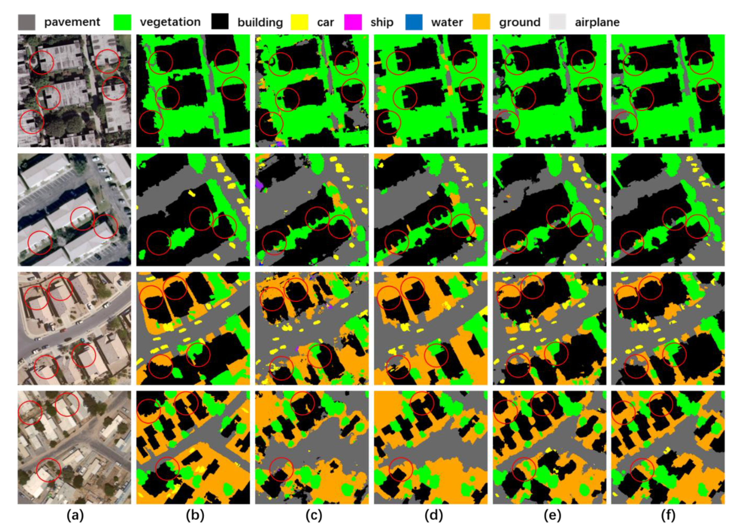
As shown in Figure 10 and Figure 11, the segmentation results of the DSSN-GCN model were significantly better than its backbone both on two datasets. In addition, there were less noise in the results of DSSN-GCN because the object-based classification reduced noises. Moreover, since the superpixel was composed of a series of adjacent pixels with consistent characteristics, which retains the boundary of the object, the results of boundaries of DSSN-GCN were more closely aligned with the real contours of the ground objects. As shown in the red circles of Figure 12, results of DSSN-GCN in (d) and (f) were better than that of (c) and (e), respectively, even the boundary in (d) and (f) fit the real boundary more closely than the ground truth (b), especially in buildings.

5. Conclusions

In order to introduce the spatial relationship information into RS image semantic segmentation, this paper proposed the DSSN-GCN framework for semantic segmentation of the RS image via combining DSSN and GCN. To lift the appearance extraction ability, we also proposed a new DSSN (AttResUNet), which had U-shaped architecture using residual blocks to encode feature maps and an attention module to refine the features. In the framework, a graph was built, where graph nodes were denoted by the superpixels. Additionally, the graph weight denoting the strength of spatial relationship was calculated by considering the spectral information and spatial information of the nodes. Then GCN combines graph node features extracted by DSSN and the graph weight to classify all the nodes, which converts the semantic segmentation into the node classification. On the basis of the DSSN-GCN framework, we designed four networks, namely DSSN-GCN V1, V2, V3 and V4. Extensive experiments performed on the UCM dataset and the DeepGlobe dataset show the effectiveness of the DSSN-GCN framework and the advance of the proposed AttResUNet. In addition, the superpixel-level modeling through GCN helped to reduce pixel-level noises and restored the boundaries of ground objects.

This paper presents that the spatial relationship information introduced by GCN enhanced the performance and robustness of classifier. The information of spatial relationship is essential for high-precision and interpretable semantic segmentation. How to effectively use spatial relationship information and other prior knowledge and learn knowledge automatically to interpret RS images intelligently requires further research in the future.

References

- Ball, J.; Anderson, D.; Chan, C.S. A Comprehensive survey of deep learning in remote sensing: Theories, tools, and challenges for the community. J. Appl. Remote Sens. 2017, 11, 042609. [Google Scholar] [CrossRef] [Green Version]
- Liu, B.; Du, S.; Du, S.; Zhang, X. Incorporating Deep Features into GEOBIA Paradigm for Remote Sensing Imagery Classification: A Patch-Based Approach. Remote Sens. 2020, 12, 3007. [Google Scholar] [CrossRef]
- Mountrakis, G.; Li, J.; Lu, X.; Hellwich, O. Deep learning for remotely sensed data. J. Photogramm. Remote Sens. 2018, 145, 1–2. [Google Scholar] [CrossRef]
- Ma, L.; Liu, Y.; Zhang, X.; Ye, Y. Deep learning in remote sensing applications: A meta-analysis and review. J. Photogramm. Remote Sens. 2019, 152, 166–177. [Google Scholar] [CrossRef]
- Li, Y.; Chen, W.; Zhang, Y.; Tao, C.; Xiao, R.; Tan, Y. Accurate cloud detection in high-resolution remote sensing imagery by weakly supervised deep learning. Remote Sens. Environ. 2020, 250, 112045. [Google Scholar] [CrossRef]
- Li, Y.; Zhang, Y.; Huang, X.; Yuille, A.L. Deep networks under scene-level supervision for multi-class geospatial object detection from remote sensing images. J. Photogramm. Remote Sens. 2018, 146, 182–196. [Google Scholar] [CrossRef]
- Zhu, X.X.; Tuia, D.; Mou, L.; Xia, G.; Zhang, L.; Xu, F.; Fraundorfer, F. Deep Learning in Remote Sensing. IEEE Geosci. Remote Sens. Lett. 2017, 5, 8–36. [Google Scholar] [CrossRef] [Green Version]
- Li, Y.; Chao, T.; Yihua, T.; Ke, S.; Jinwen, T. Unsupervised multilayer feature learning for satellite image scene classification. IEEE Geosci. Remote Sens. Lett. 2016, 13, 157–161. [Google Scholar] [CrossRef]
- Li, Y.; Ma, J.; Zhang, Y. Image retrieval from remote sensing big data: A survey. Inf. Fusion. 2021, 67, 94–115. [Google Scholar] [CrossRef]
- LeCun, Y.; Bengio, Y.; Hinton, G. Deep learning. Nature 2015, 521, 436–444. [Google Scholar] [CrossRef]
- Li, Y.; Zhang, Y.; Zhu, Z. Error-tolerant deep learning for remote sensing image scene classification. IEEE Trans. Cybern. 2020, in press. [Google Scholar] [CrossRef] [PubMed]
- Li, Y.; Zhang, Y.; Huang, X.; Ma, J. Learning source-invariant deep hashing convolutional neural networks for cross-source remote sensing image retrieval. IEEE Trans. Geosci. Remote Sens. 2018, 56, 6521–6536. [Google Scholar] [CrossRef]
- Li, Y.; Zhang, Y.; Huang, X.; Zhu, H.; Ma, J. Large-scale remote sensing image retrieval by deep hashing neural networks. IEEE Trans. Geosci. Remote Sens. 2018, 56, 950–965. [Google Scholar] [CrossRef]
- Krizhevsky, A.; Sutskever, I.; Hinton, G. Imagenet classification with deep convolutional neural networks. Commun. ACM 2017, 60, 84–90. [Google Scholar] [CrossRef]
- Basaeed, E.; Bhaskar, H.; Al-Mualla, M. Supervised remote sensing image segmentation using boosted convolutional neural networks. Knowl. Based Syst. 2016, 99, 19–27. [Google Scholar] [CrossRef]
- Camps-Valls, G.; Tuia, D.; Bruzzone, L.; Benediktsson, J.A. Advances in hyperspectral image classification. IEEE Signal Process. Mag. 2014, 31, 45–54. [Google Scholar] [CrossRef] [Green Version]
- Long, J.; Shelhamer, E.; Darrell, T. Fully convolutional networks for semantic segmentation. In Proceedings of the IEEE Conference on Computer Vision and Pattern Recognition, Boston, MA, USA, 7–12 June 2015; pp. 3431–3440. [Google Scholar]
- Noh, H.; Hong, S.; Han, B. Learning deconvolutional network for semantic segmentation. In Proceedings of the IEEE International Conference on Computer Vision, Santiago, Chile, 11–18 December 2015; pp. 1520–1528. [Google Scholar]
- Ronneberger, O.; Fischer, P.; Brox, T. U-Net: Convolutional Networks for Biomedical Image Segmentation. In Proceedings of the International Conference on Medical Image Computing and Computer Assisted Intervention, Munich, Germany, 5–9 October 2015; pp. 234–241. [Google Scholar]
- Badrinarayanan, V.; Kendall, A.; Cipolla, R. SegNet: A Deep Convolutional Encoder-Decoder Architecture for Image Segmentation. In Proceedings of the IEEE Conference on Computer Vision and Pattern Recognition, Las Vegas, NV, USA, 27–30 June 2016. [Google Scholar]
- He, K.; Gkioxari, G.; Dollár, P.; Girshick, R. Mask R-CNN. In Proceedings of the IEEE Conference on Computer Vision and Pattern Recognition, Salt Lake City, UT, USA, 18–22 June 2018. [Google Scholar]
- Chen, L.; Papandreou, G.; Kokkinos, I.; Murphy, K.; Yuille, A.L. Deeplab: Semantic image segmentation with deep convolutional nets, atrous convolution, and fully connected crfs. IEEE Trans. Pattern Anal. Mach. Intell. 2016, 40, 834–848. [Google Scholar] [CrossRef]
- Zhao, H.; Shi, J.; Qi, X.; Wang, X.; Jia, J. Pyramid Scene Parsing Network. In Proceedings of the IEEE Conference on Computer Vision and Pattern Recognition, Honolulu, HI, USA, 21–26 July 2017. [Google Scholar]
- Lin, G.; Milan, A.; Shen, C.; Reid, I. RefineNet: Multi-Path Refinement Networks for High-Resolution Semantic Segmentation. In Proceedings of the IEEE Conference on Computer Vision and Pattern Recognition, Las Vegas, NV, USA, 27–30 June 2016. [Google Scholar]
- Chen, L.; Zhu, Y.; Papandreou, G.; Schroff, F.; Adam, H. Encoder-Decoder with Atrous Separable Convolution for Semantic Image Segmentation. In Proceedings of the European Conference on Computer Vision, Munich, Germany, 8–14 September 2018. [Google Scholar]
- Roy, A.G.; Navab, N.; Wachinger, C. Concurrent Spatial and Channel ‘Squeeze & Excitation’ in Fully Convolutional Networks. In Proceedings of the International Conference on Medical Image Computing and Computer-Assisted Intervention, Granada, Spain, 16–20 September 2018. [Google Scholar]
- Hu, J.; Shen, L.; Albanie, S.; Sun, G.; Wu, E. Squeeze-and-Excitation Networks. In Proceedings of the IEEE Conference on Computer Vision and Pattern Recognition, Salt Lake City, UT, USA, 18–22 June 2018. [Google Scholar]
- Oktay, O.; Schlemper, J.; Folgoc, L.L.; Lee, M. Attention U-Net: Learning Where to Look for the Pancreas. In Proceedings of the International Conference on Medical Imaging with Deep Learning, Amsterdam, The Netherlands, 4–6 July 2018. [Google Scholar]
- Li, H.; Qiu, K.; Chen, L.; Mei, X.; Hong, L.; Tao, C. SCAttNet: Semantic Segmentation Network with Spatial and Channel Attention Mechanism for High-Resolution Remote Sensing Images. IEEE Geosci. Remote Sens. Lett. 2020, 1–5. [Google Scholar] [CrossRef]
- Woo, S.; Park, J.; Lee, J.; Kweon, I.S. CBAM: Convolutional Block Attention Module. In Proceedings of the European Conference on Computer Vision, Munich, Germany, 8–14 September 2018. [Google Scholar]
- Wurm, M.; Stark, T.; Zhu, X.X.; Weigand, M.; Taubenbock, H. Semantic segmentation of slums in satellite images using transfer learning on fully convolutional neural networks. J. Photogramm. Remote Sens. 2019, 150, 59–69. [Google Scholar] [CrossRef]
- Sherrah, J. Fully Convolutional Networks for Dense Semantic Labelling of High-Resolution Aerial Imagery. arXiv 2016, arXiv:1606.02585. [Google Scholar]
- Marmanis, D.; Wegner, J.D.; Galliani, S.; Schindler, K.; Datcu, M.; Stilla, U. Semantic segmentation of aerial images with an ensemble of CNSS. In Proceedings of the ISPRS Annals of the Photogrammetry, Remote Sensing and Spatial Information Sciences, Prague, Czech Republic, 12–19 July 2016. [Google Scholar]
- Maggiori, E.; Tarabalka, Y.; Charpiat, G.; Alliez, P. Fully Convolutional Neural Networks for Remote Sensing Image Classification. In Proceedings of the 2016 IEEE International Geoscience and Remote Sensing Symposium (IGARSS), Beijing, China, 10–15 July 2016; pp. 5071–5074. [Google Scholar]
- Kampffmeyer, M.; Salberg, A.B.; Jenssen, R. Semantic segmentation of small objects and modeling of uncertainty in urban remote sensing images using deep convolutional neural networks. In Proceedings of the IEEE Conference on Computer Vision and Pattern Recognition, Las Vegas, NV, USA, 27–30 June 2016. [Google Scholar]
- Wang, C.; Li, L. Multi-Scale Residual Deep Network for Semantic Segmentation of Buildings with Regularizer of Shape Representation. Remote Sens. 2020, 12, 2932. [Google Scholar] [CrossRef]
- Audebert, N.; Saux, B.L.; Lefèvre, S. Semantic Segmentation of Earth Observation Data Using Multimodal and Multi-Scale Deep Networks. In Proceedings of the Asian Conference on Computer Vision, Taipei, Taiwan, 20–24 November 2016; pp. 180–196. [Google Scholar]
- Zhang, M.; Hu, X.; Zhao, L.; Lv, Y.; Luo, M.; Pang, S. Learning dual multi-scale manifold ranking for semantic segmentation of high resolution images. Remote Sens. 2017, 9, 500. [Google Scholar] [CrossRef] [Green Version]
- Pan, X.; Gao, L.; Andrea, M.; Zhang, B.; Fan, Y.; Paolo, G. Semantic Labeling of High Resolution Aerial Imagery and LiDAR Data with Fine Segmentation Network. Remote Sens. 2018, 10, 743. [Google Scholar] [CrossRef] [Green Version]
- Chen, K.; Fu, K.; Gao, X.; Yan, M.; Zhang, W.; Zhang, Y.; Sun, X. Effective fusion of multi-modal data with group convolutions for semantic segmentation of aerial imagery. In Proceedings of the IEEE International Geoscience and Remote Sensing Symposium (IGARSS), Yokohama, Japan, 28 July–2 August 2019; pp. 3911–3914. [Google Scholar]
- Marmanis, D.; Schindler, K.; Wegner, J.D.; Galliani, S.; Datcu, M.; Stilla, U. Classification with an edge: Improving semantic image segmentation with boundary detection. J. Photogramm. Remote Sens. 2018, 135, 158–172. [Google Scholar] [CrossRef] [Green Version]
- Chu, H.; Shenglin, L.; Dehui, X.; Peizhang, F.; Mingsheng, L. Remote Sensing Image Semantic Segmentation Based on Edge Information Guidance. Remote Sens. 2020, 12, 1501. [Google Scholar]
- Alirezaie, M.; Längkvist, M.; Sioutis, M. Semantic referee: A neural-symbolic framework for enhancing geospatial semantic segmentation. Semant. Web. 2019, 10, 863–880. [Google Scholar] [CrossRef] [Green Version]
- Yong, L.; Wang, R.; Shan, S.; Chen, X. Structure inference net: Object detection using scene-level context and instance-level relationships. In Proceedings of the IEEE Conference on Computer Vision and Pattern Recognition, Salt Lake City, UT, USA, 18–22 June 2018; pp. 6985–6994. [Google Scholar]
- Scarselli, F.; Gori, M.; Tsoi, A.C.; Hagenbuchner, M.; Monfardini, G. The graph neural network model. IEEE Trans Neural Netw. 2009, 20, 61–80. [Google Scholar] [CrossRef] [Green Version]
- Gori, M.; Monfardini, G.; Scarselli, F. A new model for learning in graph domains. In Proceedings of the 2005 IEEE International Joint Conference on Neural Networks, Montreal, Canada, 31 July–4 August 2005. [Google Scholar]
- Kipf, T.; Welling, M. Semi-supervised classification with graph convolutional networks. In Proceedings of the international conference on learning representations, Toulon, France, 24–26 April 2017. [Google Scholar]
- Niepert, M.; Ahmed, M.; Kutzkov, K. Learning Convolutional Neural Networks for Graphs. In Proceedings of the International Conference on Machine Learning, New York, NY, USA, 19–24 June 2016. [Google Scholar]
- Li, G.; Müller, M.; Thabet, A.; Ghanem, B. DeepGCNs: Can GCNs Go as Deep as CNNs? In Proceedings of the IEEE International Conference on Computer Vision, Seoul, Korea, 27–28 October 2019. [Google Scholar]
- Veličković, P.; Cucurull, G.; Casanova, A. Graph Attention Networks. In Proceedings of the International Conference on Learning Representations, Vancouver, BC, Canada, 30 April–3 May 2018. [Google Scholar]
- Lu, Y.; Chen, Y.; Zhao, D.; Chen, J. Graph-FCN for image semantic segmentation. arXiv 2020, arXiv:2001.00335. [Google Scholar]
- Li, Y.; Chen, R.; Zhang, Y. A CNN-GCN framework for multi-label aerial image scene classification. In Proceedings of the IEEE International Geoscience and Remote Sensing Symposium (IGARSS), Hawaii, HI, USA, 19–24 July 2020. [Google Scholar]
- He, K.; Zhang, X.; Ren, S.; Sun, J. Deep residual learning for image recognition. In Proceedings of the IEEE Conference on Computer Vision and Pattern Recognition, Las Vegas, NV, USA, 27–30 June 2016. [Google Scholar]
- Shao, Z.; Yang, K.; Zhou, W.; Hu, B. Performance evaluation of single-label and multi-label remote sensing image retrieval using a dense labeling dataset. Remote Sens. 2018, 10, 964. [Google Scholar] [CrossRef] [Green Version]
- Demir, I.; Koperski, K.; Lindenbaum, D.; Pang, G.; Huang, J.; Basu, S.; Hughes, F.; Tuia, D.; Raska, R. Deepglobe 2018: A challenge to parse the earth through satellite images. In Proceedings of the 2018 IEEE/CVF Conference on Computer Vision and Pattern Recognition Workshops (CVPRW), Salt Lake City, UT, USA, 18–22 June 2018; pp. 172–17209. [Google Scholar]
- Arvor, D.; Belgiu, M.; Falomir, Z.; Mougenot, I.; Durieux, L. Ontologies to interpret remote sensing images: Why do we need them? Gisci. Remote Sens. 2019, 56, 911–939. [Google Scholar] [CrossRef] [Green Version]
- Gu, H.; Li, H.; Yan, L. An Object-Based Semantic Classification Method for High Resolution Remote Sensing Imagery Using Ontology. Remote Sens. 2017, 9, 329. [Google Scholar] [CrossRef] [Green Version]
- Garcia-Garcia, A.; Orts-Escolano, S.; Oprea, S.O.; Villena-Martinez, V.; Garcia-Rodriguez, J. A Review on Deep Learning Techniques Applied to Semantic Segmentation. arXiv 2017, arXiv:1704.06857v1. [Google Scholar]
- Achanta, R.; Shaji, A.; Smith, K. SLIC Superpixels Compared to State-of-the-art Superpixel Methods. IEEE Trans. Pattern Anal. Mach. Intell. 2012, 34, 2274–2282. [Google Scholar] [CrossRef] [PubMed] [Green Version]
Figure 1.
The workflow of the proposed deep semantic segmentation network (DSSN)-graph convolutional neural network (GCN) framework, including the DSSN module, the graph module and the GCN module. The whole process goes from top to bottom. First, the DSSN module extracts the deep features for the semantic initialization of the graph nodes. Then the graph module constructs the graph with ground objects and their spatial relationships. Finally, the GCN module combines the features and the spatial relationships in the graph to perform classification.
Figure 2.
The architecture of AttResUNet. The proposed DSSN (a) has U-shaped architecture using residual blocks (b) to encode feature maps and attention module (c) to refine the features.
Figure 3.
A toy example about the graph construction process. After the unsupervised superpixel segmentation, the remote sensing (RS) image (a) consisted of superpixels (b), which are regarded as graph nodes (c). Additionally, the first-order adjacency relationship (with common edge) between superpixels denotes graph edge (c).
Figure 4.
Visual example of the three steps in the graph convolution of GCN: information broadcasting, information collection and information aggregation. For example, node broadcasts its feature to its neighboring nodes , , and at first. Second, node collects features from node , , and . Third, aggregate information by gathering and activating nonlinearly the fusion features.
Figure 5.
Raw images and ground truth masks of the UCM dataset.
Figure 6.
Raw images and ground truth masks of the DeepGlobe dataset.
Figure 7.
Sensitivity analysis of the number of superpixels tested on the validation dataset. (a) and (b) present the change trend of OA and FWIoU with , respectively.
Figure 8.
Sensitivity analysis of the similarity factor tested on the validation dataset. (a) and (b) present the change trend of OA and FWIoU with , respectively.
Figure 9.
Sensitivity analysis of the number of GCN layers tested on the validation dataset. (a) and (b) present the change trend of OA and FWIoU with , respectively.
Figure 10.
The visible semantic segmentation of the UCM dataset. (a) and (b) are raw images and ground truth respectively. (c) and (d) are the results of U-Net and the results of DSSN-GCN V1, respectively. The results of SegNet and the results of DSSN-GCN V2 are shown on (e) and (f), respectively. (g) and (h) present the results of DeepLab V3+ and the results of DSSN-GCN V3, respectively. The results of the proposed AttResUNet and AttResUNet-GCN (DSSN-GCN V4) are displayed on (i) and (j), respectively.