Non-Cooperative Passive Direct Localization Based on Waveform Estimation

Abstract

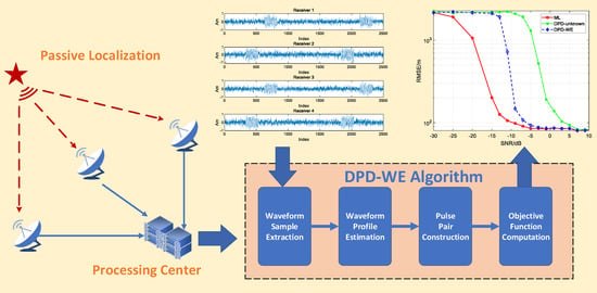
This paper considers a non-cooperative passive localization system wherein widely distributed receivers are used to localize a transmitter radiating a periodical pulse pair signal. Two possible pulse modulation models, noncoherent and coherent pulses, are fully considered for practical application, and are effectively unified as a general model for the algorithm design. To achieve highly accurate and robust localization performance, an enhanced direct position determination (DPD) algorithm based on waveform estimation (WE) is devised to jointly estimate the transmitter position and the waveform profile. The optimal objective function based on a least square (LS) principle is first derived to directly determine the position of the transmitter. Due to the complete lack of knowledge on the transmitted signal, the processing center calculates the objective function at each searched grid of interest by using estimated pulses instead of the real ones, while extraction of pulse samples and estimation of waveform are executed. Theoretical derivation gives the solution to estimate the non-parameterized waveform with a structure of maximum Rayleigh quotient. Additionally, simulation results verify the effectiveness of the proposed algorithm for many common waveform types in the cases of transmitting noncoherent and coherent pulses, and also show the excellent advantage over the classical DPD algorithm at low signal-to-noise ratio (SNR).

1. Introduction

As a fundamental demand of many applications, localization technology has been attracting great attention from radar [1,2,3,4], sonar [5,6,7], wireless sensor network [8,9,10,11], global navigation satellite systems (GNSS) [12,13,14] and so on. Generally, according to different demands of practical applications, localization systems are designed and classified into two main categories: active and passive systems. Overall, the active localization system with transmitters has better performance in accuracy and robustness than the passive one owing to its full control of transmitted signals. The passive system has the advantage of lower costs of procurement and maintenance, as well as covert operation, due to no equipment of transmitters, and thus has received significant interest in the academic community. This paper mainly considers a non-cooperative localization problem for an emitter by multiple widely distributed passive receiver stations.

The localization methods contain two main categories of indirect localization and direct localization, or sometimes called two-step and one-step localization. Common indirect localization algorithms are implemented based on some intermediate parameters, time of arrival (TOA), time difference of arrival (TDOA), direct of arrival (DOA) and Doppler shift [15,16,17,18,19,20,21], which need to be estimated from received signals in advance as inputs of the algorithms. The indirect algorithms can achieve excellent accuracy only when all the intermediate parameters are high-reliable. However, they always suffer from great performance degradation when some of intermediate parameters can not be estimated or obtained reliably from received signals, often happening in lower signal-to-noise ratio (SNR) environment. Considering the information loss that the use of intermediate parameters incurs, many direct localization algorithms are proposed to determine the position only using many raw received signals regardless of the intermediate parameters [22,23,24,25,26,27,28,29,30,31,32,33,34,35]. Compared with the indirect localization methods, the direct approaches have higher accuracy and better robustness for localization at lower SNR [22,23,24,25], as well as the inherent capability of easily localizing multiple targets [31,32,33,34,35].

Many passive direct localization algorithms have been developed to enhance performance of passive localization system, since Weiss first proposed the direct position determination (DPD) approach in [22]. Considering the use of Doppler frequency shift, Ref. [23] applied the DPD idea to multiple moving platforms for localization of a stationary emitter. In [24], a novel DPD algorithm based on cyclostationary signals was proposed to address the localization of narrowband radio transmitters in the presence of narrow interference for high robustness. For further improvement of localization accuracy at low SNR, Ref. [28] fully considered the prior knowledge about the model of a transmitted signal, and proposed a joint estimation of location and signal parameters to localize an emitter radiating linear frequency modulation (LFM) signals. Furthermore, owing to the inherent advantage of multi-target localization, some passive localization algorithms for multiple targets have evolved from the classical DPD. Ref. [31] first proposed the DPD algorithm based on multiple signals classification (MUSIC) technique for multiple unknown noncoherent signals, followed by a high resolution DPD algorithm based on minimum variance distortionless response (MVDR) [33]. To handle the invalidity for coherent signal scenario in [31,33,34] considered combining the iterative adaptive approach with DPD to localize many coherent signals. Overall, the approaches of DPD greatly promote the development of passive localization algorithms in various application scenario.

From the perspective of improving accuracy, Ref. [28] provided a novel idea to enhance the performance of the classical DPD for a passive non-cooperative localization system. Based on the assumption that transmitting signals belonged to the family of LMF, this paper first selected short time Fourier transform (STFT) technique to extract the valid spectrum fragment of the transmitting signals, and then adopted a joint estimation strategy of signal and position parameters to directly determine an emitter. The algorithm, called DPD-STFT, fully exploits the waveform profile information that the classical DPD ignores, and therefore gains better accuracy than the DPD-unknown algorithm (The DPD algorithms used in the two cases of unknown and known signal waveform are referred to as DPD-unknown and DPD-known respectively for distinction). In essence, DPD-STFT can be viewed as an attempt to approximate the optimal algorithms like DPD-known or maximum likelihood (ML) based localization algorithm. However, the premise of the known waveform model inevitably results in the practical application constraint.

In this paper, we still devote our effort to enhancing performance of DPD-unknown for better accuracy and robustness in the non-cooperative localization system. A joint estimation strategy of waveform and position is proposed to directly localize a non-cooperative emitter. Here, the restriction on the waveform model of LFM in DPD-STFT is relaxed in the proposed algorithm. Specifically, we do not make any assumption about the transmitted waveform. The proposed algorithm builds a modified position estimator for localization by replacing the true waveform with an estimated waveform, which is recovered by using a non-parameterized estimation way. Various simulation results are also given to show the performance of the proposed algorithm. The main contributions of this paper are summarized as follows:

• The proposed algorithm extends the application range of DPD-STFT algorithm due to no limitation on the waveform types of the transmitted signal.
• The proposed algorithm further considers a transmitted signal that contains periodical pulses for extension of non-cooperative passive localization, where a unified processing framework is proposed to deal with the noncoherent and coherent modulated transmitted signal.
• The proposed algorithm has the performance advantage over the classical unknown-DPD algorithm due to full exploration of waveform information.

The rest of this paper is organized as follows. A unified model for received signals with two different modulation cases is presented in Section 2. Section 3 states the localization problem formulated in a least square (LS) estimation paradigm. The proposed algorithm is presented in detail in Section 4, followed by numerical simulation results in Section 5. Finally, conclusions are drawn in Section 6.

2. Signal Model

Consider a localization system consisting of L receiving stations widely distributed in a two-dimensional Cartesian coordinate system, and the stations are located at ${\mathit{p}}_l=(x_l,y_l),l=1,2,\dots ,L$, respectively. Extension of a three-dimensional case is straightforward by increasing the dimensions of position state. The receivers are allowed to work synchronously with same reference time and phase by oscillators. They can transfer electromagnetic signals intercepted from free space to a processing center. In the surveillance region, a stationary transmitter located at $\mathit{p}=(x,y)$ radiates a periodical pulse pair signal with a fixed pulse repetition interval (PRI) $T_r$. It is assumed that the PRI is larger than the maximum time difference of arrival of the transmitting signal to the stations (This assumption means that the first received pulses of all stations correspond to the same transmitting pulse. It is a reasonable and practical assumption for simplifying the analysis). The periodical baseband signal $x\left(t\right)$ comprises of M waveforms $s\left(t\right)$ with the time width $T_p$, and is expressed as

$$x\left(t\right)=\sum _{m=0}^{M-1}s\left(t-m{T}_r\right),$$

(1)

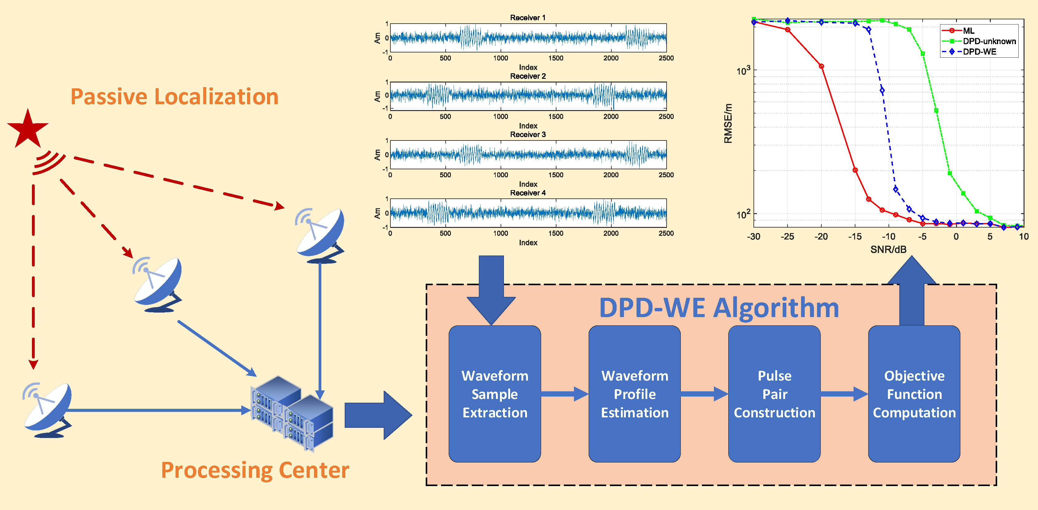
where $s\left(t\right)$ denotes the waveform embedded in each pulse duration of $x\left(t\right)$, and satisfies $s\left(t\right)=0$ for any $t\notin [0,T_p]$. As a modulation signal, $x\left(t\right)$ is modulated by multiplication with a transmitted carrier signal in a noncoherent or coherent way. Figure 1 illustrates the difference of these signals visually.

2.1. Noncoherent Pulse Pair Model

Firstly, we consider the case that the transmitter radiates a noncoherent pulse pair. For the transmitter, after noncoherent modulation to the baseband pulse pair in (1), the transmitting signal can be expressed as

$${\tilde{x}}_{\mathrm{nc}}\left(t\right)=\sum _{m=0}^{M-1}s\left(t-m{T}_r\right)e^{j{\varphi }_m}{e}^{j{\omega }_{c}t},$$

(2)

where the term ${\varphi }_m$, $m=0,\cdots ,M-1$, is starting phase of the mth modulated pulse with its value selected randomly uniformly in $[0,2\pi ]$, and ${\omega }_c=2\pi f_c$ is the angular frequency form corresponding to the carrier frequency $f_c$ of the transmitting signal.

The received signal of the receiver l can be denoted by

$$\begin{array}{c}\hfill {\tilde{r}}_{\mathrm{nc},l}\left(t\right)={\alpha }_l\sum _{m=0}^{M_l-1}s\left(t-t_0-{\tau }_l\left(\mathit{p}\right)-m{T}_r\right)e^{j{\varphi }_m}{e}^{j{\omega }_c(t-t_0-{\tau }_l\left(\mathit{p}\right))}+n_l\left(t\right),0<t<T,\end{array}$$

(3)

where ${\alpha }_l$ is the complex attenuation coefficient corresponding to the path from the transmitter to the receiver l and it is seen as a definite unknown quantity during the observation T (Assume that the wireless channel varies slowly during the observation). The term $M_l$ denotes the number of pulses that the receiver l intercepts, and the numbers of intercepted pulses from different receivers are probably unequal due to operating state of the receivers and demand of practical application. The term $t_0$ is the transmitting time of the signal from the transmitter. The term $n_l\left(t\right)$ is additive white noise, and is mutually independent between different receiving/transmitting paths. The term ${\tau }_l\left(\mathit{p}\right)$ is the delay of signal propagation from the transmitter to the receiver l, denoted by

$${\tau }_l\left(\mathit{p}\right)=\frac{\parallel \mathit{p}-{\mathit{p}}_l\parallel }{c},$$

with $\parallel •\parallel$ representing the Euclidean norm and c denoting electromagnetic wave propagation speed. Define ${\tilde{\tau }}_l(\mathit{p},t_0)={\tau }_l\left(\mathit{p}\right)+t_0$, and (3) can be written concisely as

$$\begin{array}{c}\hfill {\tilde{r}}_{\mathrm{nc},l}\left(t\right)={\alpha }_l\sum _{m=0}^{M_l-1}s\left(t-{\tilde{\tau }}_l(\mathit{p},t_0)-m{T}_r\right)e^{j{\varphi }_m}{e}^{j{\omega }_c(t-{\tilde{\tau }}_l(\mathit{p},t_0))}+n_l\left(t\right),0<t<T.\end{array}$$

(4)

Notice that, for simplifying notation, the dependence on transimitter location $\mathit{p}$ and/or work time $t_0$ is dropped so that ${\tau }_l$ and ${\tilde{\tau }}_l$ are used in place of ${\tau }_l\left(\mathit{p}\right)$ and ${\tilde{\tau }}_l(\mathit{p},t_0)$ in the remaining part of this paper.

After processing the received signal by a down-conversion mixer, we can obtain the baseband form of the received signal, expressed as

$$\begin{array}{c}\hfill r_{\mathrm{nc},l}\left(t\right)={\alpha }_l\sum _{m=0}^{M_l-1}s\left(t-{\tilde{\tau }}_l-m{T}_r\right)e^{j({\varphi }_m-{\omega }_c{\tilde{\tau }}_l)}{e}^{j{\omega }_{0}t}+n_l\left(t\right),0<t<T,\end{array}$$

(5)

where ${\omega }_0={\omega }_c-{\omega }_d$, and ${\omega }_d$ is the angular frequency of the down-conversion mixer in the receiver, known to all receivers.

2.2. Coherent Pulse Pair Model

For the case of transmitting coherent pulse pair, the transmitting signal can be expressed as

$${\tilde{x}}_c\left(t\right)=\sum _{m=0}^{M-1}s\left(t-m{T}_r\right)e^{j{\omega }_{c}t}.$$

(6)

The coherent modulation for these M pulses in the transmitter means that they have a common reference phase in time [36]. This often implies that enough information about the transmitting signal, such as reference time and phase as well as signal frequency, is necessary for the receivers to achieve coherent signal processing; however, for this case of non-cooperative localization discussed in this paper, it is too difficult, even impossible, to obtain such prior information.

For the coherent transmitted signal, the received signal of the receiver l can be denoted as

$$\begin{array}{c}\hfill {\tilde{r}}_{\mathrm{c},l}\left(t\right)={\alpha }_l\sum _{m=0}^{M_l-1}s\left(t-{\tilde{\tau }}_l-m{T}_r\right)e^{j{\omega }_c(t-{\tilde{\tau }}_l)}+n_l\left(t\right),0<t<T.\end{array}$$

(7)

Similarly, after down-conversion processing, the baseband form of the received signal that the receiver l intercepts can be expressed as

$$\begin{array}{c}\hfill r_{\mathrm{c},l}\left(t\right)={\alpha }_l\sum _{m=0}^{M_l-1}s\left(t-{\tilde{\tau }}_l-m{T}_r\right)e^{-j{w}_c{\tilde{\tau }}_l}{e}^{j{\omega }_{0}t}+n_l\left(t\right),0<t<T.\end{array}$$

(8)

2.3. Unified Signal Model

For non-cooperative localization system, the information about a transmitter, such as accurate carrier frequency, signal transmitting time and modulation method, is impossible to attain for receivers. Therefore, noncoherent processing approach is employed for designing localization algorithm. For the above noncoherent and coherent pair models, the received signal can be reconstructed in a unified model for localization due to the lack of phase information between pulses. For the noncoherent pulse pair, the Equation (5) can be rewritten as

$$\begin{array}{c}\hfill r_{\mathrm{nc},l}\left(t\right)={\alpha }_l\sum _{m=0}^{M_l-1}s\left(t-{\tilde{\tau }}_l-m{T}_r\right)e^{j{\xi }_m}{e}^{j{\omega }_0(t-{\tilde{\tau }}_l-m{T}_r)}+n_l\left(t\right),0<t<T\end{array}$$

(9)

with ${\xi }_m={\varphi }_m-{\omega }_c{\tilde{\tau }}_l+{\omega }_0({\tilde{\tau }}_l+m{T}_r)$ still distributed uniformly in $[0,2\pi ]$.

For the coherent pulse pair, we can get the similar signal form

$$\begin{array}{c}\hfill r_{\mathrm{c},l}\left(t\right)={\alpha }_l\sum _{m=0}^{M_l-1}s\left(t-{\tilde{\tau }}_l-m{T}_r\right)e^{j{\vartheta }_m}{e}^{j{\omega }_0(t-{\tilde{\tau }}_l-m{T}_r)}+n_l\left(t\right),0<t<T,\end{array}$$

(10)

where the phase ${\vartheta }_m={\omega }_0({\tilde{\tau }}_l+m{T}_r)-w_c{\tilde{\tau }}_l$ can be regarded reasonably as an unknown variable distributed uniformly in $[0,2\pi ]$ because of the lack of any prior information about the transmitter. It is worth noting that the above converted angular frequency ${\omega }_0$ is unknown to all receivers due to no precise real carrier frequency information of the transmitter.

Thus, we can unify the noncoherent and coherent received baseband signal models into the following expression

$$\begin{array}{c}\hfill r_l\left(t\right)={\alpha }_l\sum _{m=0}^{M_l-1}{e}^{j{\phi }_m}u(t-{\tilde{\tau }}_l-m{T}_r)+n_l\left(t\right),0<t<T,\end{array}$$

(11)

where

$$u\left(t\right)=s\left(t\right)e^{j{\omega }_{0}t},$$

and ${\phi }_m$, starting phase of each pulse, can be regarded as a determinate unknown variable in $[0,2\pi ]$ during the observation T. Based on this unified signal model, next, we will derive the objective function that is used to estimate the position of the transmitter.

3. Problem Formulation

In order to determine the transmitter position from the unified signal model (11), we can usually choose two approaches, the weighted least square (WLS) estimation for unknown noise distribution or the ML estimation for known exact one. As a matter of fact, they are equivalent when noise is independent white Gaussian form [37]. In this section, considering lack of the exact distribution information, an LS approach, belonging to the WLS family, is employed to estimate the position of the transmitter.

Define ${\beta }_{ml}={\alpha }_l{e}^{j{\phi }_m}$, and (11) can be rewritten as

$$\begin{array}{c}\hfill r_l\left(t\right)=\sum _{m=0}^{M_l-1}{\beta }_{ml}u(t-{\tilde{\tau }}_l-m{T}_r)+n_l\left(t\right),\end{array}$$

(12)

where ${\beta }_{ml}$ can be regarded as unknown independent variables each other since ${\alpha }_l$ and ${\phi }_m$ are independent.

Using the LS approach, we can construct a cost function about the transmitter’s position as follows

$$\begin{array}{c}\hfill C(\mathit{p},t_0,\mathbf{\beta })=\sum _{l=1}^L{C}_l(\mathit{p},t_0,{\beta }_{ml}),\end{array}$$

(13)

where

$$\begin{array}{c}\hfill C_l(\mathit{p},t_0,{\beta }_{ml})={\int }_T{\left|r_l\left(t\right)-\sum _{m=0}^{M_l-1}{\beta }_{ml}u\left(t-{\tilde{\tau }}_l-m{T}_r\right)\right|}^{2}dt,\end{array}$$

and $\mathbf{\beta }={[{\beta }_{11},\cdots ,{\beta }_{1M_1},\cdots ,{\beta }_{L1},\cdots ,{\beta }_{L{M}_L}]}^{\top }$. The superscript ${[·]}^{\top }$ represents the transpose operator. The position to be estimated exactly corresponds to the value of $\mathit{p}$ that minimizes the cost function together with the parameter vector $\mathbf{\beta }$. The minimum value of the function can be determined by making their partial derivative equal to zero for these arguments. After a series of mathematical derivation, seen in Appendix A, we can estimate the position of the transmitter by maximizing the following objective function

$$\begin{array}{c}\hfill J_0(\mathit{p},t_0)=\sum _{l=1}^L\sum _{m=0}^{M_l-1}\frac{{\left|{\int }_T{r}_l^{*}\left(t\right)u\left(t-{\tilde{\tau }}_l-m{T}_r\right)dt\right|}^2}{{\int }_T{\left|u\left(t-{\tilde{\tau }}_l-m{T}_r\right)\right|}^{2}dt}.\end{array}$$

(14)

For the periodical pulse pair signal, we denote the energy of single pulse by

$$E_s\triangleq {\int }_T{\left|s\left(t\right)\right|}^{2}dt={\int }_T{\left|u\left(t-{\tilde{\tau }}_l-m{T}_r\right)\right|}^{2}dt.$$

(15)

Since the energy term is a definite constant unrelated to the transmitter position $\mathit{p}$, the objective function in (14) can be converted to another equivalent objective function given by

$$\begin{array}{c}\hfill J(\mathit{p},t_0)=\sum _{l=1}^L\sum _{m=0}^{M_l-1}{\left|{\int }_T{r}_l^{*}\left(t\right)u\left(t-{\tilde{\tau }}_l-m{T}_r\right)dt\right|}^2.\end{array}$$

(16)

The position of the transmitter can be determined easily by searching the maximum value of (16) in three-dimensional space ($\mathit{p}$ and $t_0$) when the receivers have complete information of the transmitted signal, including waveform profile, pulse width and PRI. However, in the case of non-cooperative localization, the information about the transmitter is difficult, even impossible, to acquire. No such information means that estimating the transmitter’s position needs to solve the optimization problem

$$\begin{array}{c}\hfill \widehat{\mathit{p}}=\underset{\mathit{p},t_0,\mathcal{S}}{argmax}J(\mathit{p},t_0,\mathcal{S})=\underset{\mathit{p},t_0,\mathcal{S}}{argmax}\sum _{l=1}^L\sum _{m=0}^{M_l-1}{\left|{\int }_T{r}_l^{*}\left(t\right)u\left(t-{\tilde{\tau }}_l-m{T}_r\right)dt\right|}^2,\end{array}$$

(17)

where the defined symbol $\mathcal{S}=\{s(t,T_p),T_r,{\omega }_0\}$ includes all information about the transmitted signal. Since the modulation waveform $s(t,T_p)$ is unknown, meaning $u\left(t\right)$ is also unknown, the problem (17) can not be esaily solved only by extending the search dimensionality of parameters.

For this case of an unknown transmitted signal, the predominant challenge of solving (17) is how to treat the waveform profile. In order to avoid processing the unknown waveform directly, the DPD-unknown algorithm in [22] provided a general method of uncoupling the position parameter from the transmitted signal to determine the transmitter for passive localization. The key of this algorithm is that the Fourier transform processing of the received signals ensures the position parameter separated from the waveform profile. According to this idea and the mentioned received signal model, there is an alternative approach to solve the non-cooperative localization problem we care about. To be precise, the position can be determined by maximizing the objective function

$$Q\left(\mathit{p}\right)\triangleq \frac{{\overline{\mathit{x}}}^H\mathit{D}\left(\mathit{p}\right)\overline{\mathit{x}}}{{\overline{\mathit{x}}}^H\overline{\mathit{x}}},$$

(18)

where $\overline{\mathit{x}}$, not containing the position $\mathit{p}$, denotes the frequency samples of the transmitted signal, and $\mathit{D}\left(\mathit{p}\right)$ is a function matrix only related to the position $\mathit{p}$. Then, the transmitter position can be obtained by determining the maximum Rayleigh quotient of (18), and the detailed explanation can be seen in Appendix B.

However, for the widely-used pulse pair signal, especially in radar application, the DPD approach will suffer from a certain performance loss. Generally, two main factors should be responsible for the performance loss. Firstly, the pulse class signal usually contains massive pure noise parts without useful waveform signals, which interferes the estimation of the true transmitted signal in the DPD-unknown algorithm, and further impacts negatively on the localization accuracy. Additionally, regardless of the inner period constraint between each pulse of the pulse pair signal, localizing the transmitter by simply employing the DPD-unknown algorithm is often not an appropriate approach for the high-accuracy position determination in low SNR. Based on the above arguments, we propose a novel algorithm that sufficiently excavates the property of a periodical signal to improve the localization accuracy for the non-cooperative localization system.

4. The Localization Algorithm Based on Waveform Estimation

Although the unknown waveform $u\left(t\right)$ plagues the application of the estimator in (17) for determining the transmitter position, we can still consider to approximate the estimator via replacing the true waveform $u\left(t\right)$ with an estimated $\widehat{u}\left(t\right)$. It is because extracting the waveform samples from received signals is available theoretically and practically according to time sequence relation of delays. On the other hand, these received periodical pulses can provide abundant waveform samples to guarantee high accuracy of the estimation. This means that we can accomplish the localization in (17) by building the processing procedure of extraction, estimation and reconstruction for the waveform $u\left(t\right)$.

For the ability to handle signals in the digital processing system, we can rewrite the estimator as the discrete version

$$\begin{array}{c}\hfill \widehat{\mathit{p}}=\underset{\mathit{p},t_0,\mathcal{S}}{argmax}\sum _{l=1}^L\sum _{m=0}^{M_l-1}{\left|{\mathit{r}}_l^H{\mathit{u}}_{ml}(\mathit{p},t_0,\mathcal{S})\right|}^2,\end{array}$$

(19)

where

$$\begin{array}{cc}\hfill & {\mathit{r}}_l\triangleq {[r_l\left(0\right),r_l\left(1\right),\cdots ,r_l(N_s-1)]}^{\top },\hfill \\ \hfill & {\mathit{u}}_{ml}(\mathit{p},t_0,\mathcal{S})\triangleq {[u_{ml}\left(0\right),u_{ml}\left(1\right),\cdots ,u_{ml}(N_s-1)]}^{\top },\hfill \\ \hfill & r_l\left(k\right)\triangleq r_l\left(k{T}_s\right),u_{ml}\left(k\right)\triangleq u\left(k{T}_s-{\tilde{\tau }}_l-m{T}_r\right).\hfill \end{array}$$

$T_s$ and $N_s$ are the sample interval and number of the samples respectively.

Now, the basic problem we face is how to estimate the transmitter position $\mathit{p}$ by employing the estimator in (19) under the condition of no knowledge about the transmitted signal $\mathcal{S}$ and the transmitting time $t_0$. Here, a grid search computation method is still employed in the estimator (19) due to no analytical solution to the position $\mathit{p}$. According to the idea mentioned above, what we need to do firstly is to extract the samples of $u\left(t\right)$, which is incorporated in the each pulse of the received signals by the determinate time sequence relationship of delay and PRI. Therefore, interception of true waveforms can be achieved by searching for potential delay, PRI and $t_0$.

For notational convenience, we define the search parameter set $\mathbf{\theta }\triangleq (\mathit{p},t_0,T_p,T_r)$, and it can uniquely determine the results of extracted waveform samples. After obtaining the samples, we can employ an LS-based approach to estimate the waveform $u\left(t\right)$, and further reconstruct the signal $\widehat{\mathcal{S}}\left(\mathbf{\theta }\right)$ to replace the true one $\mathcal{S}$. Finally, substituting the true pulse ${\mathit{u}}_{ml}(\mathit{p},t_0,\mathcal{S})$ in (19) with the estimated one ${\widehat{\mathit{u}}}_{ml}(\mathit{p},t_0,\widehat{\mathcal{S}}\left(\mathbf{\theta }\right))$, namely ${\widehat{\mathit{u}}}_{ml}\left(\mathbf{\theta }\right)$, we can determine the transmitter position by

$$\begin{array}{c}\hfill \widehat{\mathit{p}}=\underset{\mathbf{\theta }}{argmax}\sum _{l=1}^L\sum _{m=0}^{M_l-1}{\left|{\mathit{r}}_l^H{\widehat{\mathit{u}}}_{ml}\left(\mathbf{\theta }\right)\right|}^2,\end{array}$$

(20)

where ${\widehat{\mathit{u}}}_{ml}\left(\mathbf{\theta }\right)$ is the pulse signal reconstructed by the estimated waveform $\widehat{u}(t,\mathbf{\theta })$ and the time sequence relationship that the searched $t_0$ and $\mathit{p}$ determines. The true parameter $\mathbf{\theta }$ means completely exact extraction and estimation for the waveform profile, which implies considerably large objective function value. Therefore, the transmitter position can be obtained by searching for $\mathbf{\theta }$ that maximizes the approximate objective function below

$$\begin{array}{c}\hfill \tilde{J}\left(\mathbf{\theta }\right)=\sum _{l=1}^L\sum _{m=0}^{M_l-1}{\left|{\mathit{r}}_l^H{\widehat{\mathit{u}}}_{ml}\left(\mathbf{\theta }\right)\right|}^2.\end{array}$$

(21)

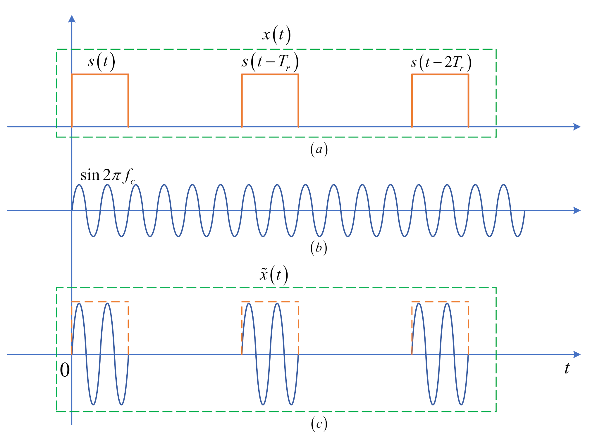
The brief flowchart of the estimation for the transmitter position is shown in Figure 2. Since this localization algorithm is direct for the position estimate, we call it direct position determination based on waveform estimation (DPD-WE).

Next, we will introduce and discuss this algorithm in detail from three component parts: extraction of waveform samples, and estimation of waveform, as well as design and analysis of DPD-WE algorithm.

4.1. Extraction of Waveform Samples

As shown in the process of Figure 2, one of the crucial procedures is how to extract many waveform samples from the all received pulse pair signals. The exact extraction of samples is an essential prerequisite for correct estimation of the waveform. Here, the extraction method is based on the fact that these pulses reappear periodically with a fixed interval in received signal. Extraction of pulse samples is implemented according to their delay relationship in the pair signals in every parameter search.

For a specific search parameter $\mathbf{\theta }$, where $\mathit{p}$, $t_0$, $T_p$ and $T_r$ are all fixed, we define the starting and terminal time of the mth extracted pulse in the observed signal $r_l\left(t\right)$ as

$$\begin{array}{ccc}\hfill & t_{l,m}^{\mathrm{s}}\left(\mathbf{\theta }\right)& \triangleq {\tau }_l\left(\mathit{p}\right)+t_0+(m-1)T_r,\hfill \end{array}$$

(22)

$$\begin{array}{ccc}\hfill & t_{l,m}^{\mathrm{e}}\left(\mathbf{\theta }\right)& \triangleq {\tau }_l\left(\mathit{p}\right)+t_0+T_p+(m-1)T_r.\hfill \end{array}$$

(23)

The above time is determined completely by the searched position coordinate $\mathit{p}$, transmitting time $t_0$, pulse width $T_p$ and PRI $T_r$. From (22) and (23), it is known that the width of every extracted pulse is consistent, equal to $T_p$. The discrete sample indexes of the starting and terminal time can be computed respectively as

$$\begin{array}{c}\hfill n_{l,m}^{\mathrm{s}}\left(\mathbf{\theta }\right)=⌈\frac{t_{l,m}^{\mathrm{s}}\left(\mathbf{\theta }\right)}{T_s}⌉,\end{array}$$

(24)

$$\begin{array}{c}\hfill n_{l,m}^{\mathrm{e}}\left(\mathbf{\theta }\right)=⌊\frac{t_{l,m}^{\mathrm{e}}\left(\mathbf{\theta }\right)}{T_s}⌋,\end{array}$$

(25)

where $\lceil ·\rceil$, $\lfloor ·\rfloor$ represent the operations of rounding towards plus infinity and minus infinity respectively. The length of the sample is obtained by

$$N_{l,m}\left(\mathbf{\theta }\right)=⌊\frac{t_{l,m}^{\mathrm{s}}\left(\mathbf{\theta }\right)-t_{l,m}^{\mathrm{e}}\left(\mathbf{\theta }\right)}{T_s}⌋=⌊\frac{T_p}{T_s}⌋,$$

(26)

or computed by $N_{l,m\left(\mathbf{\theta }\right)}=n_{l,m}^{\mathrm{s}}\left(\mathbf{\theta }\right)-n_{l,m}^{\mathrm{e}}\left(\mathbf{\theta }\right)$. It is noted that the length of all extracted pulses for all receivers is identical in one parameter search, and it only depends on the parameter $T_p$. Thus, $N_{l,m}\left(\mathbf{\theta }\right)$ can be denoted by $N\left(T_p\right)$ directly.

According to the time above, the mth extracted waveform from the received signal ${\mathit{r}}_l$ can be denoted by the below vector

$$\begin{array}{c}\hfill {\mathit{r}}_{l,m}^{\mathrm{s}}\left(\mathbf{\theta }\right)={\mathit{r}}_l\left[n_{l,m}^{\mathrm{s}}\left(\mathbf{\theta }\right):n_{l,m}^{\mathrm{e}}\left(\mathbf{\theta }\right)\right],m=1,2,\cdots ,M_l\left(\mathbf{\theta }\right),\end{array}$$

(27)

where ${\mathit{r}}_l\left[A:B\right]$ is the operation of extracting the elements from the A-th to B-th indexes in the vector ${\mathit{r}}_l$, and ${\mathit{r}}_{l,m}^{\mathrm{s}}\left(\mathbf{\theta }\right)\in {\mathbb{C}}^{N\left(T_p\right)\times 1}$. $M_l\left(\mathbf{\theta }\right)$ stands for the number of the extracted waveforms. The number is computed according to the observing time T and searched period $T_r$. After fully considering integrity of extracted pulses, the number can be expressed by

$$\begin{array}{c}\hfill M_l\left(\mathbf{\theta }\right)\triangleq \left\{\begin{array}{cc}{p}_l\left(\mathbf{\theta }\right),\hfill & q_l\left(\mathbf{\theta }\right)<d\hfill \\ p_l\left(\mathbf{\theta }\right)+1,\hfill & q_l\left(\mathbf{\theta }\right)\ge d\hfill \end{array}\right.\end{array}$$

(28)

with

$$d\triangleq \frac{T_p}{T_r}$$

and

$$\begin{array}{ccc}\hfill & p_l\left(\mathbf{\theta }\right)\triangleq ⌊\frac{T-{\tau }_l\left(\mathit{p}\right)-t_0}{T_r}⌋,& q_l\left(\mathbf{\theta }\right)\triangleq \frac{T-{\tau }_l\left(\mathit{p}\right)-t_0}{T_r}-p_l\left(\mathbf{\theta }\right).\hfill \end{array}$$

Note that $T_p<T_r<T$. $p_l\left(\mathbf{\theta }\right)$ and $q_l\left(\mathbf{\theta }\right)$ stand for the number of the captured integral pulse signal and the remaining non-integral part normalized by $T_r$ respectively. $p_l\left(\mathbf{\theta }\right)$ and d are defined together to judge whether the last extracted pulse is complete. The number of extracted samples is treated as $p_l\left(\mathbf{\theta }\right)+1$ if the remaining non-integral part is more than the width of the intercepted pulse, otherwise it is equal to $p_l\left(\mathbf{\theta }\right)$. It is worth noting that the waveform sample is extracted in a multi-pulse signal as if it were in a single pulse signal, when the search value of $T_r$ is selected as the observing time T.

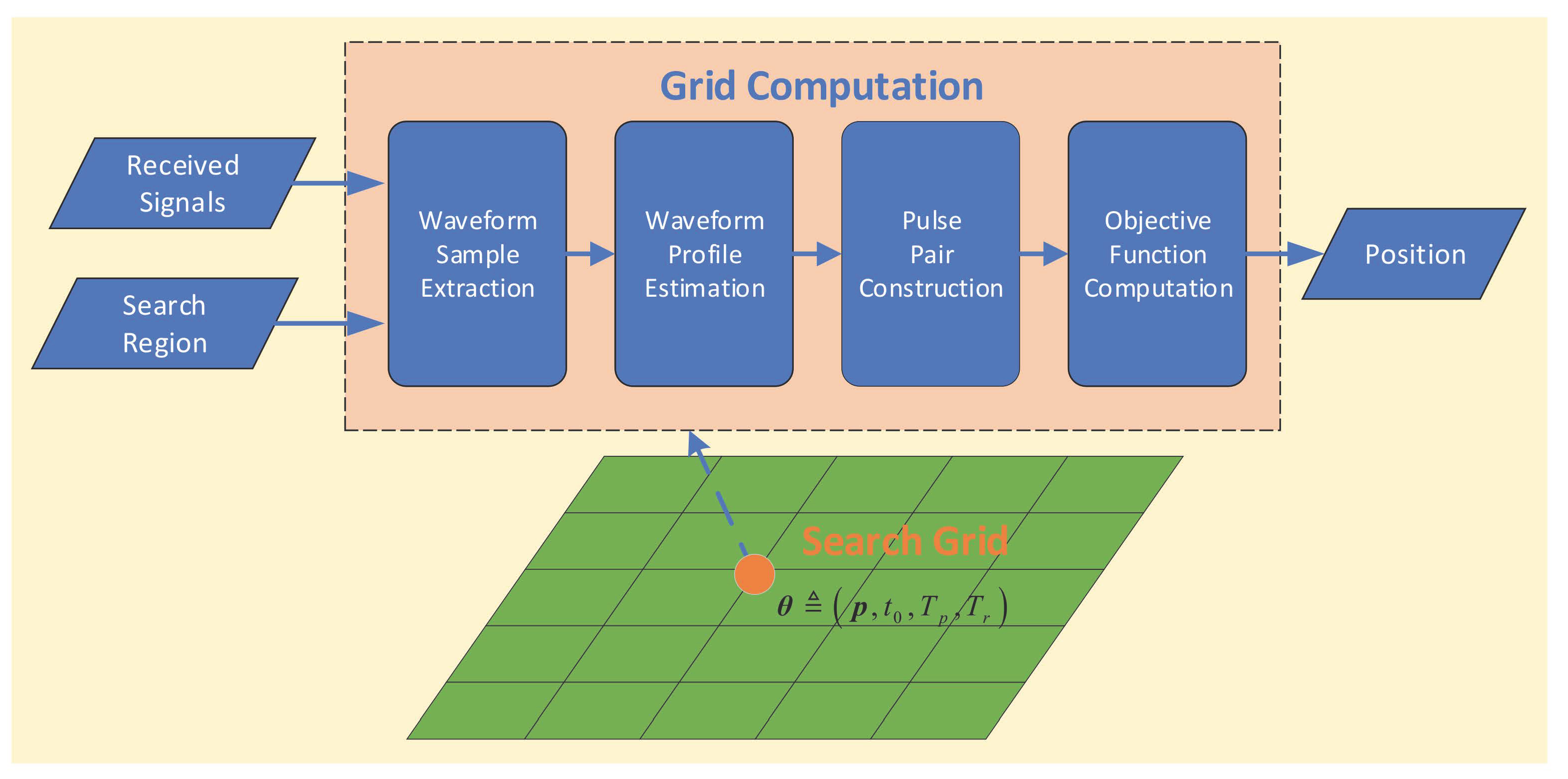
The indexes $n_{l,m}^{\mathrm{s}}\left(\mathbf{\theta }\right)$, $n_{l,m}^{\mathrm{e}}\left(\mathbf{\theta }\right)$ and the sample number $M_l\left(\mathbf{\theta }\right)$ are related to $\mathbf{\theta }$, and hence the extracted sample group ${\mathit{r}}_{l,m}^{\mathit{s}}\left(\mathbf{\theta }\right)$ varies in size and number with different searched pulse width and PRI. But, the length of all samples for L received pulse pair signals still remains identical for the certain search parameter. It is easily known that all the extracted samples will contain complete signal waveform without loss if the hypothetical $\mathbf{\theta }$ responds to the true transmitter position $\mathit{p}$, transmitting time $t_0$, pulse width $T_p$ and repetition period $T_r$. With regard to a correct hypothetical $\mathbf{\theta }$, the process of extracting samples is illustrated on Figure 3.

Considering all L receivers, the total amount of the extracted waveform samples is

$$M\left(\mathbf{\theta }\right)=\sum _{l=1}^L{M}_l\left(\mathbf{\theta }\right).$$

We assemble all $M\left(\mathbf{\eta }\right)$ extracted samples in a signal sample matrix as,

$$\mathit{S}\left(\mathbf{\theta }\right)\triangleq \left[{\mathit{r}}_{1,1}^{\mathrm{s}}\left(\mathbf{\theta }\right),\cdots ,{\mathit{r}}_{l,m}^{\mathrm{s}}\left(\mathbf{\theta }\right),\cdots ,{\mathit{r}}_{L,M_L\left(\mathbf{\theta }\right)}^{\mathrm{s}}\left(\mathbf{\theta }\right)\right].$$

(29)

For compact representation, $\mathit{S}\left(\mathbf{\theta }\right)$ is written as

$$\mathit{S}\left(\mathbf{\theta }\right)=[{\mathit{r}}_1^{\mathrm{s}}\left(\mathbf{\theta }\right),\cdots ,{\mathit{r}}_{M\left(\mathbf{\theta }\right)}^{\mathrm{s}}\left(\mathbf{\theta }\right)],$$

where $\mathit{S}\left(\mathbf{\theta }\right)\in {\mathbb{C}}^{N\left(T_p\right)\times M\left(\mathbf{\theta }\right)}$. Note that the size of the matrix $\mathit{S}\left(\mathbf{\theta }\right)$ depends on $\mathbf{\theta }$. As for the correct $\mathbf{\theta }$, the whole waveform information about the transmitting signal is embodied in this matrix. For the purpose of completely determining the modified function $\tilde{J}\left(\mathbf{\theta }\right)$, we still need to estimate the waveform $\widehat{u}(t,\mathbf{\theta })$ based on the sample matrix $\mathit{S}\left(\mathbf{\theta }\right)$ next.

4.2. Estimation of Waveform Based on the LS Approach

In order to obtain $\tilde{J}\left(\mathbf{\theta }\right)$, this subsection will describe how to estimate the waveform $\widehat{u}(t,\mathbf{\theta })$ in detail. Since completely no knowledge about the parameter model of the waveform can be utilized, we need to build a non-parameterized signal model for the estimation. According to the sample group $\mathit{S}\left(\mathbf{\theta }\right)$, the extracted signal model can be built as

$${\mathit{r}}_m^{\mathrm{s}}\left(\mathbf{\theta }\right)={\alpha }_m\left(\mathbf{\theta }\right)\mathit{u}\left(\mathbf{\theta }\right)+{\mathbf{\nu }}_m\left(\mathbf{\theta }\right),m=1,\cdots ,M\left(\mathbf{\theta }\right),$$

(30)

where $\mathit{u}\left(\mathbf{\theta }\right)$ is an implicit mathematical model corresponding to samples of the waveform extracted at $\mathbf{\theta }$. It is necessarily noted that the model $\mathit{u}\left(\mathbf{\theta }\right)$ varies with the search parameter $\mathbf{\theta }$, which means that the signal model can keep consistent with all extracted samples only when the search parameter $\mathbf{\theta }$ better tallies with the true ones. Such consistency can guarantee correct estimation for the waveform, and on the contrary inconsistent one can not achieve it. That could be seen in the next simulation illustration. Moreover, ${\alpha }_m\left(\mathbf{\theta }\right)$ is an unknown determinate complex coefficient corresponding to $\mathit{u}\left(\mathbf{\theta }\right)$, and ${\mathbf{\nu }}_m\left(\mathbf{\theta }\right)$ represents noise term contained in the samples. For conciseness of writing, $\mathbf{\theta }$ in ${\mathit{r}}_m^{\mathrm{s}}\left(\mathbf{\theta }\right)$, ${\alpha }_m\left(\mathbf{\theta }\right)$, $\mathit{u}\left(\mathbf{\theta }\right)$, and ${\mathbf{\nu }}_m\left(\mathbf{\theta }\right)$ will be dropped without impact of understanding.

Define some matrices as follows,

$$\begin{array}{ccc}\mathit{R}& =& \left[{\mathit{r}}_1^{\mathrm{s}},\cdots ,{\mathit{r}}_{M\left(\mathbf{\theta }\right)}^{\mathrm{s}}\right],\\ \mathit{V}& =& \left[{\mathbf{\nu }}_1,\cdots ,{\mathbf{\nu }}_{M\left(\mathbf{\theta }\right)}\right],\\ \mathbf{\alpha }& =& {\left[{\alpha }_1,\cdots ,{\alpha }_{M\left(\mathbf{\theta }\right)}\right]}^{\top },\end{array}$$

and (30) can be represented as

$$\mathit{R}=\mathit{u}{\mathbf{\alpha }}^{\top }+\mathit{V}.$$

(31)

To estimate the non-parameterized waveform $\mathit{u}$ without any distribution knowledge of the noise term as well, the LS approach is employed. The waveform can be estimated by solving the following optimization problem

$$\underset{\mathit{u},\mathbf{\alpha }}{min}{∥\mathit{R}-\mathit{u}{\mathbf{\alpha }}^{\top }∥}_F^2,$$

(32)

where ${\parallel •\parallel }_F$ represents the Frobenius norm. Using the relationship between trace and Frobenius norm of matrix, the optimization problem in (32) is equivalent to

$$\underset{\mathit{u},\mathbf{\alpha }}{min}\mathrm{tr}\left[{(\mathit{R}-\mathit{u}{\mathbf{\alpha }}^{\top })}^H(\mathit{R}-\mathit{u}{\mathbf{\alpha }}^{\top })\right],$$

(33)

where $\mathrm{tr}(•)$ represents trace operation of matrix. The detailed derivation of the analytic solution to the problem (33) is shown in Appendix C, where the estimate of the waveform is given by

$$\begin{array}{c}\hfill \widehat{\mathit{u}}=\underset{\mathit{u}}{max}\frac{{\mathit{u}}^H\mathit{R}{\mathit{R}}^H\mathit{u}}{{\parallel \mathit{u}\parallel }^2}.\end{array}$$

(34)

This is a classical problem of maximum Rayleigh quotient. Thus, we can obtain the estimated waveform

$$\begin{array}{c}\hfill \widehat{\mathit{u}}={\mathit{v}}_{{\lambda }_{max}\left(\mathit{R}{\mathit{R}}^H\right)},\end{array}$$

(35)

where ${\mathit{v}}_{{\lambda }_{max}\left(\mathit{R}{\mathit{R}}^H\right)}$ denotes the eigenvector corresponding to the maximum eigenvalue of $\mathit{R}{\mathit{R}}^H$.

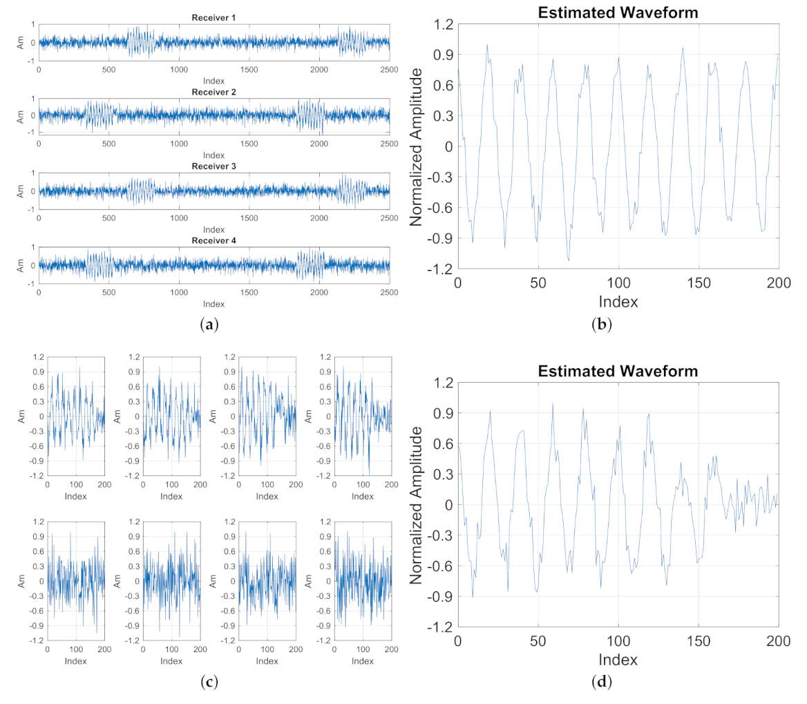
An example of waveform estimation is given in Figure 4, where the estimation is implemented according to 8 extracted pulse samples. As proposed above, extracted samples have two different cases: one is that all samples follow an identical signal model (consistent samples) and the other is that they come from different signal models (inconsistent samples). The former estimation provides the foundation for accurately estimating the waveform, shown in Figure 4b, while the latter, corresponding to an incorrect search parameter $\mathbf{\theta }$, results in terrible extraction and estimation, shown in Figure 4c,d respectively. Therefore, a correct search parameter can guarantee samples consistent in model, and exactly based on that, we can construct the true pulse ${\mathit{u}}_{ml}\left(\mathbf{\theta }\right)$ by the accurate estimated waveform $\widehat{u}(t,\mathbf{\theta })$. Next, we will discuss how to utilize the objective function $\tilde{J}\left(\mathbf{\theta }\right)$ to estimate the position of the transmitter.

4.3. Design and Analysis of DPD-WE Algorithm

In the above subsection, we obtain the waveform estimate $\widehat{u}(t,\mathbf{\theta })$ by the LS approach conditioned at $\mathbf{\theta }$, and thus the pulse ${\mathit{u}}_{ml}\left(\mathbf{\theta }\right)$ can be reconstructed as the estimate form ${\widehat{\mathit{u}}}_{ml}\left(\mathbf{\theta }\right)$ according to the searched starting and terminal time $t_{l,m}^{\mathrm{s}}\left(\mathbf{\theta }\right)$ and $t_{l,m}^{\mathrm{s}}\left(\mathbf{\theta }\right)$. Using the pulse ${\widehat{\mathit{u}}}_{ml}\left(\mathbf{\theta }\right)$, the position of the transmitter can be determined by maximizing the function $\tilde{J}\left(\mathbf{\theta }\right)$. On the other hand, ${\widehat{\mathit{u}}}_{ml}\left(\mathbf{\theta }\right)$ has a non-zero value only in the part of pulse duration, and therefore $\tilde{J}\left(\mathbf{\theta }\right)$ in (21) can be further simplified in computation as

$$\begin{array}{c}\hfill \tilde{J}\left(\mathbf{\theta }\right)=\sum _{l=1}^L\sum _{m=0}^{M_l-1}{\left|{\mathit{r}}_{l,m}^H\left(\mathbf{\theta }\right){\widehat{\mathit{u}}}_{ml}\left(\mathbf{\theta }\right)\right|}^2,\end{array}$$

(36)

where ${\mathit{r}}_{l,m}\left(\mathbf{\theta }\right)$ is an intercepted segment of ${\mathit{r}}_l$ in time, corresponding to the non-zero part of the mth pulse ${\widehat{\mathit{u}}}_{ml}\left(\mathbf{\theta }\right)$ at the lth receiver.

Additionally, it can be seen from (36) that a wider searched width obviously causes a larger function value, which can affect the estimation performance of the position. The reason is that the intercepted signal will contain pure noise part besides the waveform when the searched width is larger than the true one. It will further result in the inclusion of the noise part in the estimated waveform. Eventually, $\tilde{J}\left(\mathbf{\theta }\right)$ will obtain a larger value owing to the contribution of noise energy. In order to solve this problem, a power coefficient is defined by

$$P\left(\mathbf{\theta }\right)\triangleq \frac{\Vert {\widehat{\mathit{u}}}_{ml}\left(\mathbf{\theta }\right){\Vert }^2}{T_p},$$

(37)

where $\Vert {\widehat{\mathit{u}}}_{ml}\left(\mathbf{\theta }\right){\Vert }^2$ is energy of the estimated waveform ${\widehat{\mathit{u}}}_{ml}\left(\mathbf{\theta }\right)$ during searched $T_p$. The power coefficient is a function of $\mathbf{\theta }$, and is expected to yield a larger value at correct $T_p$ than at other longer searched pulse width since the waveform signal has more power than noise.

Considering the contribution of the power coefficient, we can modify the objective function $\tilde{J}\left(\mathbf{\theta }\right)$ using

$${\tilde{J}}_{\mathrm{mod}}\left(\mathbf{\theta }\right)\triangleq P\left(\mathbf{\theta }\right)\tilde{J}\left(\mathbf{\theta }\right).$$

(38)

Hence, the estimator of the transmitter position is given by

$$\widehat{\mathbf{\theta }}=\underset{\mathbf{\theta }}{argmax}{\tilde{J}}_{\mathrm{mod}}\left(\mathbf{\theta }\right).$$

(39)

A complete realization of DPD-WE algorithm is given by Algorithm 1. Furthermore, the analysis of robustness and computation load for the proposed algorithm is discussed as follows.

Algorithm 1: Realization of DPD-WE Algorithm

Tolerance to Searched Pulse Width From the basic idea of DPD-WE, it can be seen that the algorithm mainly contains two essential parts: extraction and estimation of waveforms, where the extracted results are determined completely by search parameters. In the extraction procedure, the consistency of samples highly relies on the search parameters $t_0$, $\mathit{p}$ and $T_r$, where $T_r$ mainly determines the number of extracted waveform samples from one received signal. $T_p$ only impacts on the pulse width of extracted samples. Actually, the consistency is the key to accurately estimate and reconstruct waveform for successful localization, and thus $t_0$, $\mathit{p}$ and $T_r$ play more crucial roles than $T_p$ in correctness assurance for the localization. It can be explained from the perspective of geometrical localization. With regard to $T_p$, whether the width matches the true one or not, the localization can be completed effectively as long as the width ensures enough SNR of the intercepted signal. In fact, to a certain extent, it can affect the localization performance by controlling signal processing gain, where an intercepted pulse width determines how much proportion of signal and noise energy is obtained. It is this property that makes the DPD-WE algorithm have strong tolerance to non-accurate searched pulse width; this conclusion will be verified in next simulation experiments.

Computation Complexity From the realization of DPD-WE in Algorithm 1, we can see that the computation cost of DPD-WE is dominated by calculation of $\tilde{J}\left(\mathbf{\theta }\right)$, which refers to a high-dimensional grid search. It is worth noting the search ranges of $\mathbf{\theta }$ can be determined in advance according to prior information, such as surveillance region of interest, a practical application for the specific type of a target and demand of localization accuracy. For the parameter space with $N_{t_0}$ emission time, $N_{T_p}$ pulse width and $N_{T_r}$ PRI candidates, plus 2-D coordinates, the computation load of the algorithm is bounded by $\mathcal{O}\left(N_{t_0}{N}_{T_p}{N}_{T_r}{N}_x{N}_y\right)$ at single receiver, where $N_x$, $N_y$ denotes the amounts of grids in x and y respectively. Considering all receivers, the proposed algorithm involves the total computation complexity of about $\mathcal{O}\left(L{N}_{t_0}{N}_{T_p}{N}_{T_r}{N}_x{N}_y\right)$. As proposed above, the algorithm has excellent tolerance to range of $T_p$, and thus the computation load can be alleviated enormously by decreasing search quantity of $T_p$. Therefore, practical computation load is limited to the order of $\mathcal{O}\left(N_{t_0}{N}_{T_r}{N}_x{N}_y\right)$, meanwhile considering that the total amount L of receivers is generally considerably small. Additionally, for the purpose of improving computational efficiency, a parallel computation strategy can be applied in the process of implementation because of the independence of different grid for computation of $\tilde{J}\left(\mathbf{\theta }\right)$.

5. Simulation Results

In this section, we first show by numerical simulation how the searched pulse width works on the waveform estimation and further affects the localization performance in the proposed DPD-WE method. Then we examine its effectiveness for three kinds of transmitted waveform signals, and meanwhile verify its superiority over the traditional DPD approach by Monte Carlo experiments.

As a common quality criterion of parameter estimation performance, root mean square error (RMSE) is selected to evaluate localization accuracy, defined by

$$RMSE=\sqrt{\frac{1}{N-1}{\sum }_{i=1}^N{({\widehat{x}}_i-x)}^2+{({\widehat{y}}_i-y)}^2},$$

where $({\widehat{x}}_i,{\widehat{y}}_i)$ denotes the estimated position of the transmitter in the ith localization test with a total amount of N experiments, and $(x,y)$ is the actual transmitter position.

5.1. Impact of Searched Pulse Width on Localization

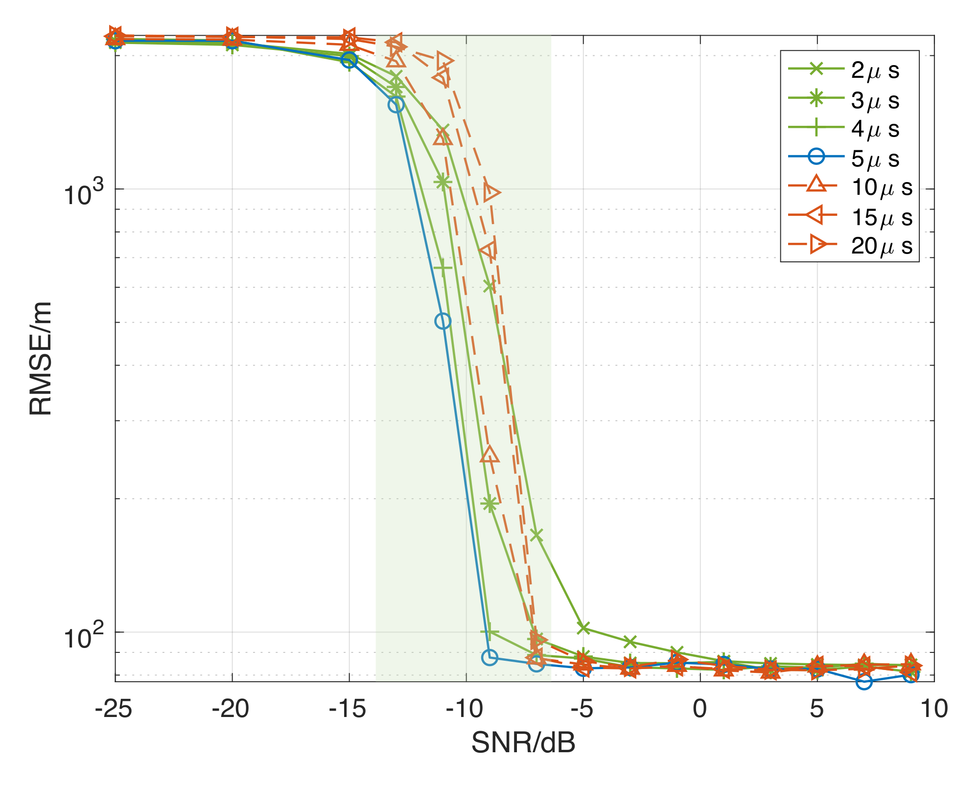
As discussed in previous section, the proposed DPD-WE algorithm has strong tolerance to searched pulse width, and here we validate the impact of width on localization performance using a numerical experiment. Three different cases of extracted pulse widths, equal to, smaller and larger than the true width, are selected to show visually how the widths effect waveform estimation. Then, the results of RMSE against SNR are provided to assess the impact of different searched width.

In this simulation, four receivers at $(-10,0)\mathrm{km}$, $(10,0)\mathrm{km}$, $(0,-10)\mathrm{km}$ and $(0,10)\mathrm{km}$ respectively are deployed to localize a transmitter located at $(0,0)\mathrm{km}$, which emits a noncoherent periodical pulse pair signal at $t_0=10\mathsf{\mu }\mathrm{s}$ with PRI $T_r=150\mathsf{\mu }\mathrm{s}$ and pulse width $T_p=5\mathsf{\mu }\mathrm{s}$. During the pulses, a Gaussian profile is modulated in the carrier signal of $f_c=2\mathrm{GHz}$, and single transmitted pulse signal is given by

$$s_1\left(t\right)={\left(\frac{1}{T_p^2}\right)}^{\frac{1}{4}}exp\left(-\frac{\pi t^2}{T_p^2}\right)exp\left(j2\pi f_{c}t\right),0\le t\le T_p.$$

Assume that received signals can be converted down to the baseband frequency $f_0=0.5\mathrm{MHz}$ by a down-conversion mixer according to approximate spectral knowledge using spectrum estimation technique. The received signals in baseband are sampled at $F_s=10\mathrm{MHz}$, and the observing time is set as $T=1\mathrm{ms}$.

For the Gaussian waveform, we first display the waveform estimation results in three cases of ${\widehat{T}}_p=3\mathsf{\mu }\mathrm{s}$, ${\widehat{T}}_p=5\mathsf{\mu }\mathrm{s}$ and ${\widehat{T}}_p=10\mathsf{\mu }\mathrm{s}$ on the premise that the other search parameters perfectly match the true. Figure 5a is a diagram of one pulse from a received signal, where three kinds of colors are used to distinguish the interception schemes with red, green and orange rectangles representing the schemes of ${\widehat{T}}_p=3\mathsf{\mu }\mathrm{s}$, ${\widehat{T}}_p=5\mathsf{\mu }\mathrm{s}$ and ${\widehat{T}}_p=10\mathsf{\mu }\mathrm{s}$ respectively. Figure 5b–d show the estimated waveform profiles corresponding to these interception scheme, where the time windows of these three plots are set as the same range for the convenience of comparison.

From Figure 5b, we can see that only partial waveform information can be recovered by the waveform estimation approach when intercepted pulse width is smaller than the true width. This intercepted scheme actually means that the transmitted signal is regarded as another different pulse pair signal that has shorter pulse width than the true transmitting signal. In contrast with case 1, the estimated waveform corresponding to case 3 is wider than the true pulse width, shown in Figure 5d, because the intercepted samples contain pure noise signal besides complete waveform signal. Only in case 2 does the intercepted width match the true width perfectly, and thus it can obtain most complete waveform information, shown in Figure 5c. In fact, whether the intercepted width is equal to, smaller or larger than the true, we can recover correct waveform information from these consistent samples by the LS-based estimation approach, and effectively execute the localization for the transmitter. How these three interception schemes affect localization performance is mainly reflected in how much signal processing gain can be obtained, which is shown in the next numerical experiment.

To verify the tolerance of DPD-WE to the pulse width we are searching for, we test the localization performance of the algorithm for the transmitter at many SNR environments in a wide range of searched widths. The algorithm is executed based on grid computation by searching for $t_0$, $\mathit{p}$ and $T_r$ of interest at different given searched pulse widths. Figure 6 shows the RMSE of the estimated positions in 1000 independent localization experiments, in each of which the transmitter appears randomly within the rectangle region of ${[-0.5,0.5]}^{1\times 2}{\mathrm{km}}^2$. According to the Figure 6, it is fundamentally concluded that the algorithm can achieve considerably high accuracy at sufficient SNR, no matter what pulse widths are chosen. However, there are still some performance differences between them at low SNRs, marked by the green rectangle in the plot. Generally speaking, wider searched pulse width can obtain smaller RMSE when the width is smaller than the true one. On the contrary, larger searched width results in a large RMSE when the width is wider than the true one. This phenomenon can be explained from the perspective of signal processing gain. Intercepting the consistent waveform samples within the true pulse generally ensures that these samples do not contain any part of pure noise, which means that a widely intercepted width can collect more waveform energy than a narrow intercepted width. Therefore, the localization performance with such searched widths improves with the width increasing, and will reach the top when complete waveform samples not containing any pure noise is intercepted sufficiently, exactly corresponding to the case that searched width equals to the true. On the other hand, a searched width larger than the true width definitely causes intercepting extra pure noise without exception. The redundant noise will reduce SNR of the estimated signal, and further impair the localization performance. Fortunately, different searched pulse widths only have a limited impact on the performance, which happens mainly in lower SNR. Consequently, in practical applications, we can implement localization only by using an appropriate searched width, which is easily selected by few tests.

5.2. Localization Performance Comparison

In this subsection, we further examine the localization performance by comparing with the classical DPD approach [22] and the ML-based localization method, which is chosen as a low bound of performance due to its asymptotic efficiency. The ML-based algorithm is implemented under the assumption that all knowledge about the transmitted signal, such as emission time, waveform, pulse width, PRI and so on, is perfectly known to the receivers, and the detailed derivation about it is shown in Appendix D.

Additionally, three different kinds of waveform profiles, Gaussian, linear frequency modulation (LFM) and rectangle waveform, are also used to test the performance in the cases of noncoherent and coherent modulation respectively. The simulation parameters still remain the same as the previous ones except the waveform profiles. The transmitted pulses with the other two waveform profiles, LFM and rectangle, are given by

$$s_2\left(t\right)=exp\left(\frac{j\pi B{t}^2}{T_p}\right)exp\left(j2\pi f_{c}t\right),0\le t\le T_p,$$

with modulated bandwidth $B=1$ MHz, and by

$$s_3\left(t\right)=exp\left(j2\pi f_{c}t\right),0\le t\le T_p,$$

respectively.

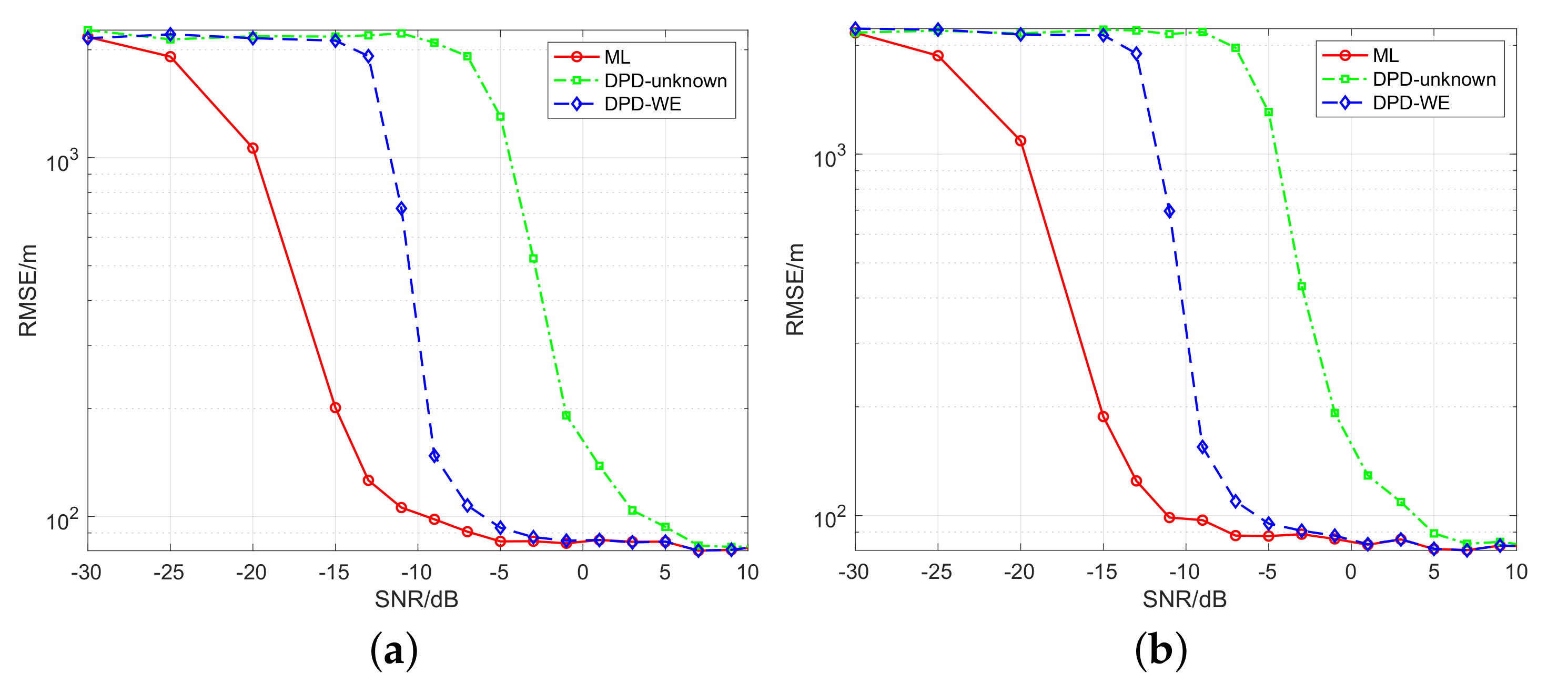
The Figure 7 shows the RMSEs of the ML-based localization, DPD-unknown and DPD-WE methods against SNR for the Gaussian pulse pair signal, where Figure 7a,b correspond to the noncoherent and coherent cases respectively. It is seen from the two plots that RMSEs of these localization methods decrease with SNR rising, and will keep unchanged at considerably low level after SNR becomes sufficiently large. It is worth noting that the low bound of RMSE is limited by the size of grid since the grid computation is employed, and it can be adjusted according to the demand for practical localization accuracy. Figure 7a,b show that the proposed DPD-WE algorithm can achieve almost completely similar accuracy for noncoherent and coherent cases and successfully localize the transmitter at sufficient SNR. It exactly tallies with the proposed signal processing approach, where the received pulses are processed noncoherently due to unknown knowledge about these pulses, including modulated phases.

On the other hand, compared with the classical DPD-unknown algorithm, DPD-WE can acquire the performance advantage of around 8 dB in moderate and low SNR, which means that the proposed algorithm has stronger noise tolerance and higher accuracy than the DPD-unknown. The performance gain that DPD-WE obtains mainly results from full exploitation of waveform information by only extracting useful parts of the received signals. Therefore, the interference of noise is reduced significantly. Additionally, from these two plots, we can also see that the ML localization algorithm has most excellent performance owing to utilizing complete and exact knowledge about the transmitted signal. The difference between the ML and DPD-WE algorithms is caused by coherent processing gain and perfect match for the waveform profile. In fact, DPD-WE has the potential to approach the ML algorithm in performance as well if the identical knowledge of the transmitted signal is given.

Additionally, for the Gaussian transmitted signal, Figure 8 also shows the localization performance of three methods in the case of only receiving a single pulse, where the observing time is set as $T=250\mathsf{\mu }\mathrm{s}$. The simulation result demonstrates that DPD-WE has the same performance advantage over DPD-unknown, which means that DPD-WE can be applied to the scenario of single pulse.

Finally, we further examine the localization performance for the other waveform profiles. Figure 9 and Figure 10 give the localization results of three algorithms in the cases of transmitting LFM and rectangle pulses respectively. Similar localization performance with the Gaussian pulse is also seen in these two types of waveform profiles for noncoherent and coherent modulation. Only slight performance distinctions are expressed between $-10$ dB and $-5$ dB due to the difference of waveform profiles. It means that the proposed algorithm can be applied to a wide variety of waveform profiles for non-cooperative passive localization.

6. Conclusions

In this paper, a non-cooperative passive localization system with widely distributed receivers has been discussed to determine a transmitter emitting a periodical pulse signal. Firstly, we introduce two possible pulse models of noncoherent and coherent modulation in detail, and then unify them as a general model for further localization. Based on the unified model, a localization algorithm combined with waveform estimation approach is proposed to determine the transmitter without any knowledge requirement about the transmitted signal. Simulation results show that the proposed method can tackle the localization problem for the noncoherent and coherent transmitted pulses, and achieve a great advantage over the classical DPD-unknown method in accuracy and robustness at low SNR. Extension to the scenario of multiple emitters is a worthy direction of further study for the proposed algorithm.

References

- Godrich, H.; Haimovich, A.M.; Blum, R.S. Target localization accuracy gain in MIMO radar-based systems. IEEE Trans. Inf. Theory 2010, 56, 2783–2803. [Google Scholar] [CrossRef] [Green Version]
- He, Q.; Hu, J.; Blum, R.S.; Wu, Y. Generalized Cramér–Rao bound for joint estimation of target position and velocity for active and passive radar networks. IEEE Trans. Signal Process. 2016, 64, 2078–2089. [Google Scholar] [CrossRef]
- Niu, R.; Blum, R.S.; Varshney, P.K.; Drozd, A.L. Target localization and tracking in noncoherent multiple-input multiple-output radar systems. IEEE Trans. Aerosp. Electron. Syst. 2012, 48, 1466–1489. [Google Scholar] [CrossRef] [Green Version]
- Guo, S.; Zhao, Q.; Cui, G.; Li, S.; Kong, L.; Yang, X. Behind Corner Targets Location Using Small Aperture Millimeter Wave Radar in NLOS Urban Environment. IEEE J. Sel. Top. Appl. Earth Obs. Remote Sens. 2020, 13, 460–470. [Google Scholar] [CrossRef]
- Marani, G.; Choi, S.K. Underwater target localization. IEEE Robot. Autom. Mag. 2010, 17, 64–70. [Google Scholar] [CrossRef]
- Coraluppi, S. Multistatic sonar localization. IEEE J. Ocean. Eng. 2006, 31, 964–974. [Google Scholar] [CrossRef]
- Rui, L.; Ho, K. Efficient closed-form estimators for multistatic sonar localization. IEEE Trans. Aerosp. Electron. Syst. 2015, 51, 600–614. [Google Scholar] [CrossRef]
- Wymeersch, H.; Lien, J.; Win, M.Z. Cooperative localization in wireless networks. Proc. IEEE 2009, 97, 427–450. [Google Scholar] [CrossRef]
- Win, M.Z.; Shen, Y.; Dai, W. A theoretical foundation of network localization and navigation. Proc. IEEE 2018, 106, 1136–1165. [Google Scholar] [CrossRef]
- Shit, R.C.; Sharma, S.; Puthal, D.; Zomaya, A.Y. Location of Things (LoT): A review and taxonomy of sensors localization in IoT infrastructure. IEEE Commun. Surv. Tutor. 2018, 20, 2028–2061. [Google Scholar] [CrossRef]
- Laoudias, C.; Moreira, A.; Kim, S.; Lee, S.; Wirola, L.; Fischione, C. A survey of enabling technologies for network localization, tracking, and navigation. IEEE Commun. Surv. Tutor. 2018, 20, 3607–3644. [Google Scholar] [CrossRef] [Green Version]
- Hegarty, C.J.; Chatre, E. Evolution of the global navigation satellite system (GNSS). Proc. IEEE 2008, 96, 1902–1917. [Google Scholar] [CrossRef]
- Seco-Granados, G.; López-Salcedo, J.; Jiménez-Baños, D.; López-Risueño, G. Challenges in Indoor Global Navigation Satellite Systems: Unveiling its core features in signal processing. IEEE Signal Process. Mag. 2012, 29, 108–131. [Google Scholar] [CrossRef]
- Closas, P.; Gusi-Amigo, A. Direct position estimation of GNSS receivers: Analyzing main results, architectures, enhancements, and challenges. IEEE Signal Process. Mag. 2017, 34, 72–84. [Google Scholar] [CrossRef]
- Shen, J.; Molisch, A.F.; Salmi, J. Accurate passive location estimation using TOA measurements. IEEE Trans. Wirel. Commun. 2012, 11, 2182–2192. [Google Scholar] [CrossRef]
- Malanowski, M.; Kulpa, K. Two methods for target localization in multistatic passive radar. IEEE Trans. Aerosp. Electron. Syst. 2012, 48, 572–580. [Google Scholar] [CrossRef]
- Wang, Y.; Ho, K. TDOA positioning irrespective of source range. IEEE Trans. Signal Process. 2016, 65, 1447–1460. [Google Scholar] [CrossRef]
- Wang, Y.; Ho, K. An asymptotically efficient estimator in closed-form for 3-D AOA localization using a sensor network. IEEE Trans. Wirel. Commun. 2015, 14, 6524–6535. [Google Scholar] [CrossRef]
- Sun, Y.; Ho, K.; Wan, Q. Eigenspace solution for AOA localization in modified polar representation. IEEE Trans. Signal Process. 2020, 68, 2256–2271. [Google Scholar] [CrossRef]
- Nguyen, N.H.; Doğançay, K. Closed-form algebraic solutions for 3-D Doppler-only source localization. IEEE Trans. Wirel. Commun. 2018, 17, 6822–6836. [Google Scholar] [CrossRef]
- Jia, T.; Ho, K.; Wang, H.; Shen, X. Effect of sensor motion on time delay and Doppler shift localization: Analysis and solution. IEEE Trans. Signal Process. 2019, 67, 5881–5895. [Google Scholar] [CrossRef]
- Weiss, A.J. Direct position determination of narrowband radio frequency transmitters. IEEE Signal Process. Lett. 2004, 11, 513–516. [Google Scholar] [CrossRef]
- Amar, A.; Weiss, A.J. Localization of narrowband radio emitters based on Doppler frequency shifts. IEEE Trans. Signal Process. 2008, 56, 5500–5508. [Google Scholar] [CrossRef]
- Reuven, A.M.; Weiss, A.J. Direct position determination of cyclostationary signals. Signal Process. 2009, 89, 2448–2464. [Google Scholar] [CrossRef]
- Weiss, A.J. Direct geolocation of wideband emitters based on delay and Doppler. IEEE Trans. Signal Process. 2011, 59, 2513–2521. [Google Scholar] [CrossRef]
- Bosse, J.; Krasnov, O.; Yarovoy, A. Direct target localization and deghosting in active radar network. IEEE Trans. Aerosp. Electron. Syst. 2015, 51, 3139–3150. [Google Scholar] [CrossRef]
- Xia, W.; Xia, X.; Li, H.; Liu, W.; Hu, J.; He, Z. A noise-constrained distributed adaptive direct position determination algorithm. Signal Process. 2017, 135, 9–16. [Google Scholar] [CrossRef]
- Yi, W.; Chen, Z.; Hoseinnezhad, R.; Blum, R.S. Joint estimation of location and signal parameters for an LFM emitter. Signal Process. 2017, 134, 100–112. [Google Scholar] [CrossRef]
- Picard, J.S.; Weiss, A.J. Direct Position Determination Sensitivity to NLOS Propagation Effects on Doppler-Shift. IEEE Trans. Signal Process. 2019, 67, 3870–3881. [Google Scholar] [CrossRef]
- Zhang, S.; Huang, Z.; Feng, X.; He, J.; Shi, L. Multi-Sensor Passive Localization Using Direct Position Determination with Time-Varying Delay. Sensors 2019, 19, 1541. [Google Scholar] [CrossRef] [Green Version]
- Weiss, A.J.; Amar, A. Direct position determination of multiple radio signals. EURASIP J. Adv. Signal Process. 2005, 2005, 653549. [Google Scholar] [CrossRef] [Green Version]
- Bosse, J.; Ferréol, A.; Larzabal, P. A spatio-temporal array processing for passive localization of radio transmitters. IEEE Trans. Signal Process. 2013, 61, 5485–5494. [Google Scholar] [CrossRef]
- Tirer, T.; Weiss, A.J. High Resolution Direct Position Determination of Radio Frequency Sources. IEEE Signal Process. Lett. 2016, 23, 192–196. [Google Scholar] [CrossRef]
- Zhou, T.; Yi, W.; Kong, L. Direct position determination of multiple coherent sources using an iterative adaptive approach. Signal Process. 2019, 161, 203–213. [Google Scholar] [CrossRef]
- Yi, W.; Zhou, T.; Ai, Y.; Blum, R.S. Suboptimal low complexity joint multi-target detection and localization for non-coherent MIMO radar with widely separated antennas. IEEE Trans. Signal Process. 2020, 68, 901–916. [Google Scholar] [CrossRef]
- Richards, M.A. Fundamentals of Radar Signal Processing, 2nd ed.; McGraw-Hill Education: Berkshire, UK, 2014. [Google Scholar]
- Kay, S.M. Fundamentals of Statistical Signal Processing; Prentice Hall PTR: Lebanon, IN, USA, 1993. [Google Scholar]
Figure 1.
Illustration of the concept of a coherent transmitting signal. (a) Modulation pulse pair . (b) Carrier Signal. (c) Coherent transmitting signal.
Figure 2.
A flow graph for direct position determination (DPD)-waveform estimation (WE) algorithm Based on grid computation.
Figure 3.
The extraction process of samples in a received pulse pair signal measurement at the correct hypothetical with and . (a) Received signal contaminated by noise with signal-to-noise ratio (SNR) 10 dB. (b) Extracted samples of the first pulse by (27) at the hypothetical .
Figure 4.
The estimation results of the transmitted Gaussian waveform at the completely correct hypothetical and a wrong hypothetical for all pulse pair signals with and . (a) All received signal measurements with two pulses at SNR 5 dB. (b) Estimate of the waveform at the correct hypothetical . (c) All intercepted pulses corresponding to a wrong hypothetical . (d) Estimate of the waveform at the wrong hypothetical .
Figure 5.
Illustration of a received signal and estimation results according to different intercepted pulse widths. (a) A diagram of three types of interception cases in single received pulse. (b–d) Estimated waveform corresponding to the following intercepted width of: (b) cases 1: . (c) case 2: . (d) case 3: .
Figure 6.
Root mean square errors (RMSEs) of estimated positions corresponding to different searched width cases against SNR from dB to 10 dB.
Figure 7.
RMSE vs. SNR for the three localization algorithms of maximum likelihood (ML), DPD-unknown and DPD-WE with transmitting Gaussian pulses of noncoherent and coherent modulations: (a) noncoherent modulation, (b) coherent modulation.
Figure 8.
RMSE vs. SNR for the three localization algorithms of ML, DPD-unknown and DPD-WE with transmitting single Gaussian pulse.
Figure 9.
RMSE vs. SNR for the three localization algorithms of ML, DPD-unknown and DPD-WE with transmitting LFM pulses of noncoherent and coherent modulations: (a) noncoherent modulation, (b) coherent modulation.
Figure 10.
RMSE vs. SNR for the three localization algorithms of ML, DPD-unknown and DPD-WE with transmitting rectangle pulses of noncoherent and coherent modulations: (a) noncoherent modulation, (b) coherent modulation.
Publisher’s Note: MDPI stays neutral with regard to jurisdictional claims in published maps and institutional affiliations. |
© 2021 by the authors. Licensee MDPI, Basel, Switzerland. This article is an open access article distributed under the terms and conditions of the Creative Commons Attribution (CC BY) license (http://creativecommons.org/licenses/by/4.0/).
Share and Cite
MDPI and ACS Style
Zhou, T.; Yi, W.; Kong, L. Non-Cooperative Passive Direct Localization Based on Waveform Estimation. Remote Sens. 2021, 13, 264. https://0-doi-org.brum.beds.ac.uk/10.3390/rs13020264
AMA Style
Zhou T, Yi W, Kong L. Non-Cooperative Passive Direct Localization Based on Waveform Estimation. Remote Sensing. 2021; 13(2):264. https://0-doi-org.brum.beds.ac.uk/10.3390/rs13020264
Chicago/Turabian StyleZhou, Tao, Wei Yi, and Lingjiang Kong. 2021. "Non-Cooperative Passive Direct Localization Based on Waveform Estimation" Remote Sensing 13, no. 2: 264. https://0-doi-org.brum.beds.ac.uk/10.3390/rs13020264
Note that from the first issue of 2016, this journal uses article numbers instead of page numbers. See further details here.