DR-Net: An Improved Network for Building Extraction from High Resolution Remote Sensing Image

Abstract

At present, convolutional neural networks (CNN) have been widely used in building extraction from remote sensing imagery (RSI), but there are still some bottlenecks. On the one hand, there are so many parameters in the previous network with complex structure, which will occupy lots of memories and consume much time during training process. On the other hand, low-level features extracted by shallow layers and abstract features extracted by deep layers of artificial neural network cannot be fully fused, which leads to an inaccurate building extraction from RSI. To alleviate these disadvantages, a dense residual neural network (DR-Net) was proposed in this paper. DR-Net uses a deeplabv3+Net encoder/decoder backbone, in combination with densely connected convolution neural network (DCNN) and residual network (ResNet) structure. Compared with deeplabv3+net (containing about 41 million parameters) and BRRNet (containing about 17 million parameters), DR-Net contains about 9 million parameters; So, the number of parameters reduced a lot. The experimental results for both the WHU Building Dataset and Massachusetts Building Dataset, DR-Net show better performance in building extraction than other two state-of-the-art methods. Experiments on WHU building data set showed that Intersection over Union (IoU) increased by 2.4% and F1 score increased by 1.4%; in terms of Massachusetts Building Dataset, IoU increased by 3.8% and F1 score increased by 2.9%.

1. Introduction

There are many applications for automatically extracting buildings from remote sensing images (RSI), such as urban planning, population estimation, disaster emergency response, etc. [1]. However, automatically assigning each pixel in RSI into buildings or non-buildings is a challenging task, because there are large within-class and small between-class variance in pixel values of objects. There are big differences in the size and shape of buildings. At the same time, there is a strong similarity between buildings and non-buildings. With the development of artificial neural network technology, neural network structure [2,3,4,5,6,7,8,9], and the operation of convolution, pooling, batch normalization, and other calculation methods [4,5,6,10,11,12,13,14,15] have made a great progress. These developments have helped CNN [16] surpass conventional methods in various computer vision tasks, such as object detection, semantic and instance segmentation, etc. [17]. Therefore, CNN is also used in the field of object extraction from RSI. Ball [18] comprehensively discussed the progress and challenge in extracting objects from RSI using deep learning methods. In this paper, we focus on the building extraction from RSI; we only talk about the application of CNN in building extraction, which can be summarized as the following three methods.

The first method is based on image classification task with CNN. A fixed-size image tile is putted into a CNN and predict the classes of one or several pixels in the center of the tile [19,20]. This idea is called sliding-window-based method, because it uses a sliding window travers all over the RSI at a certain step to acquire the fixed-size image tile, and then obtains segmentation result of the entire image. However, this method will cause a lot of repetitive computation and seriously affects the efficiency of image segmentation. In order to reduce the impact of repeated calculations, a new idea consisting of proposal regions and sliding window convolutional neural network algorithm was proposed [21,22], but the proposal regions will influence the results. The second method is called object-oriented convolutional neural network semantic segmentation which combines image segmentation with neural network classification. This method consists of two steps. First, conventional image segmentation methods such as multi-scale segmentation are used to segment the image into potential object patches, and then compress, stretch, and fill these potential object patches to meet the input size of the neural network. Second, these image patches are inputted into the neural network for training and classification [23,24]. However, deep learning methods are not used in the image segmentation process, and the bottleneck problem of image segmentation is not alleviated. The accuracy of the image segmentation seriously affects image semantic segmentation. The third method is called semantic segmentation and is based on fully convolutional neural network (FCN) [25]. The basic idea of the FCN is to replace the fully connected layers with the convolutional layers, so that the final feature map contains position information. Moreover, in order to improve the spatial resolution of the feature map, the last layer of the convolutional neural network is up sampled to the same size as the input image. FCN is an end-to-end deep learning network for image semantic segmentation. It does depend on manual-designed features and makes it possible to realize semantic segmentation tasks through autonomous extracting semantic features from images.

At present, most CNNs used to extract buildings from RSI are still based on the idea of FCN. In order to improve the accuracy and the speed of network training, some researchers have proposed many neural network structures [26,27,28,29,30,31,32] for the semantic segmentation of RSI.

To improve the results of building extraction, the features extracted by both shallow layers and deep layers are merged. Most of the methods fusing shallow features and deep features use residual networks and skip-layer connections. In [26], a new FCN structure consisting of a spatial residual convolution module named spatial residual inception (SRI) was proposed for extracting buildings from RSI. In [33], residual network connection was also used for building extraction. In [34], Following the basic architecture of U-net [2], a deep convolutional neural network named DeepResUnet was proposed, which can effectively perform urban building segmentation at pixel scale from RSI and generate accurate segmentation results. In [27], based on U-net [2] a new network named ResUnet-a was proposed, which was in combination with hole convolution, residual connection method, pyramid pooling and multi-task learning mechanism, but the fusion of deep and shallow features in the residual block is not enough.

Another way to improve the performance of building extraction is to make full use of the multi-scale features of the pixels. Based on this idea, multi-scale feature extractors were used to the deep neural networks, such as a global multi-scale encoder-decoder network (GMEDN) [28], U-shaped hollow pyramid pooling (USPP) network [29], ARC-Net [33], and ResUnet-a [30]. These network structures contribute to extracted and fused the multi-scale feature information of pixels in the decoding module. However, in order to control the number of parameters in the neural network, these networks only add the multi-scale feature extractor in the decoding module. Lacking the fusion of deep and shallow features in the encoding stage has an adverse effect on the building extraction.

To improve the result of building extraction, some scholars further modified the output results of the CNN. Based on the U-net and residual neural network, BRRNet [31] was proposed, which is composed of a prediction module and a result adjustment network. The adjustment network takes the probability map outputted by the prediction module as input, and then outputs the final semantic segmentation result. However, BRRNet does not adopt depth separable convolution, batch normalization, and other strategies, so there are still numerous parameters. Another new strategy [32] combining neural network with polygon regularization was used to build the extraction. It consists of two steps: firstly, a neural network preliminarily extracts buildings from RSI, and then regularized polygons are used to correct the buildings extracted by the neural network. The first step has a big influenced on the final result. Thus, it is necessary to improve the performance of the neural network.

Some scholars applied multi-task learning [27,35] and attention mechanism neural network structure [36,37] to build the extraction from RSI. However, introducing more effective feature fusion and multi-scale information extraction strategies into multi-task learning and attention mechanism neural networks can further improve the effect.

At present, in order to reduce training parameters and improve training speed of the neural network, on the one hand, depth separable convolution and hole convolution were used to replace the conventional convolution operation, and on the other hand, batch normalization processing was introduced to accelerate the convergence speed of the network. In order to reduce the training parameters in the network, we adopt the method that reduces the number of convolution kernels in densely connected networks.

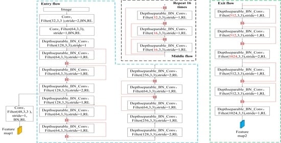
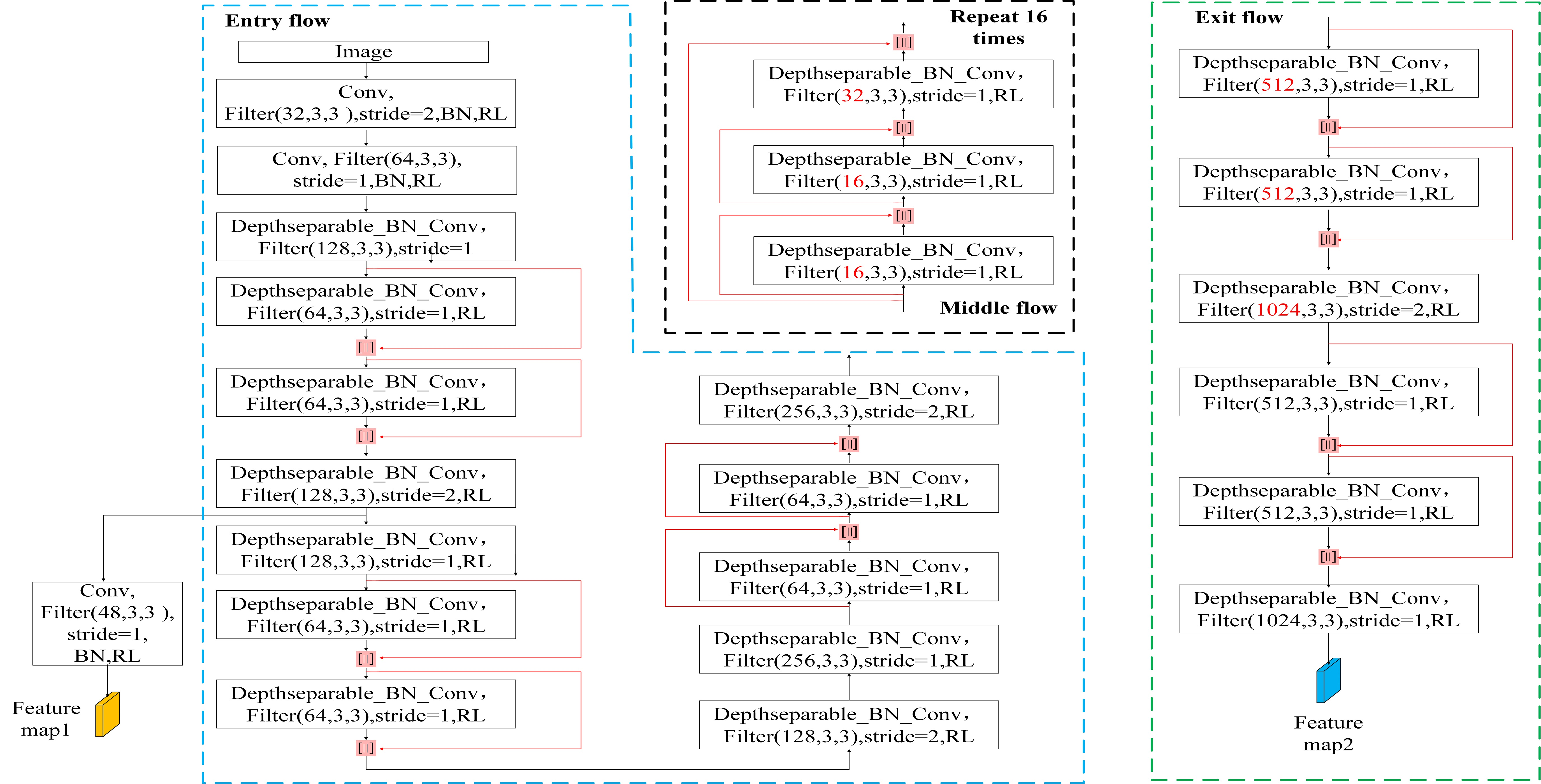
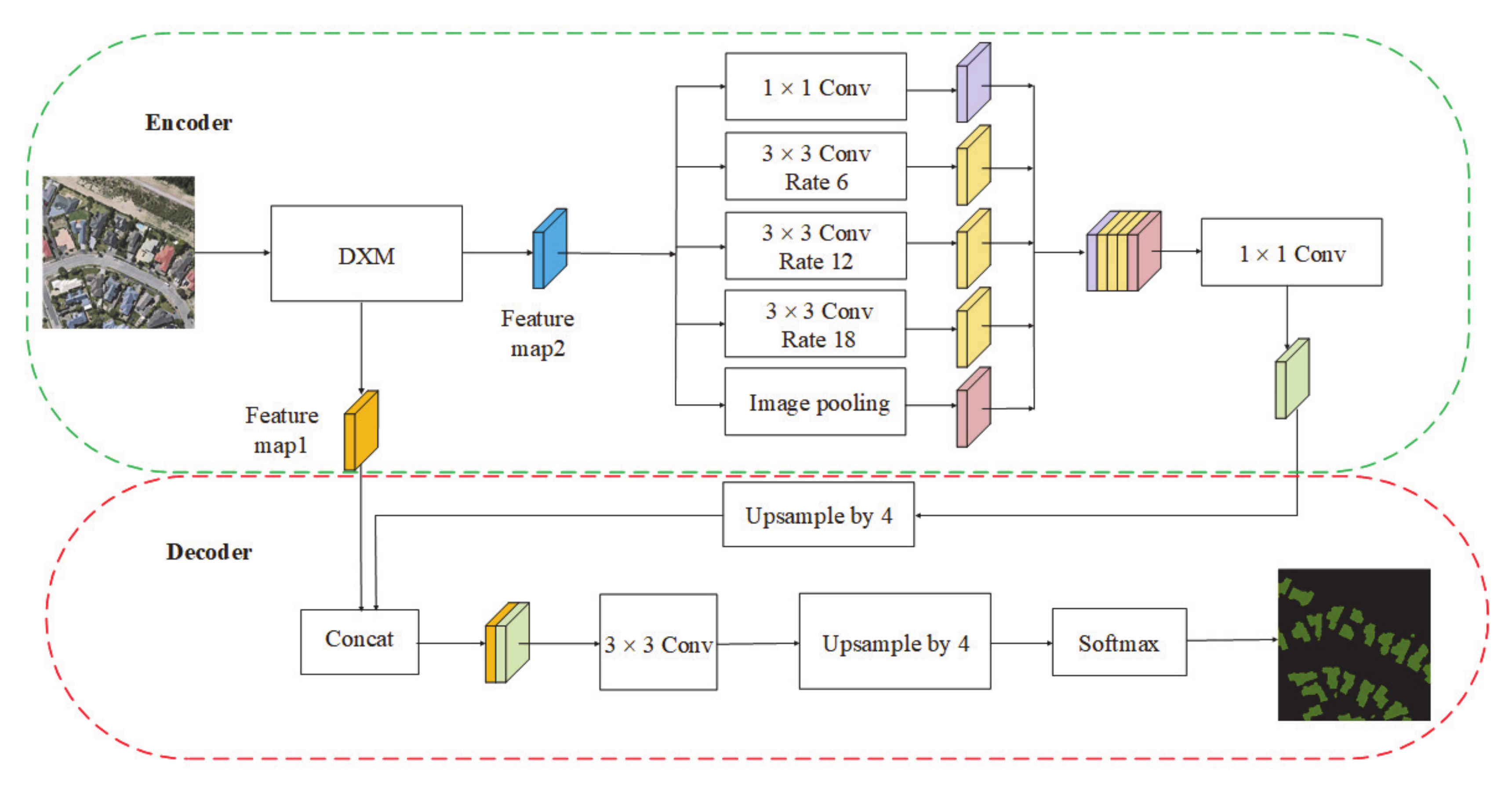
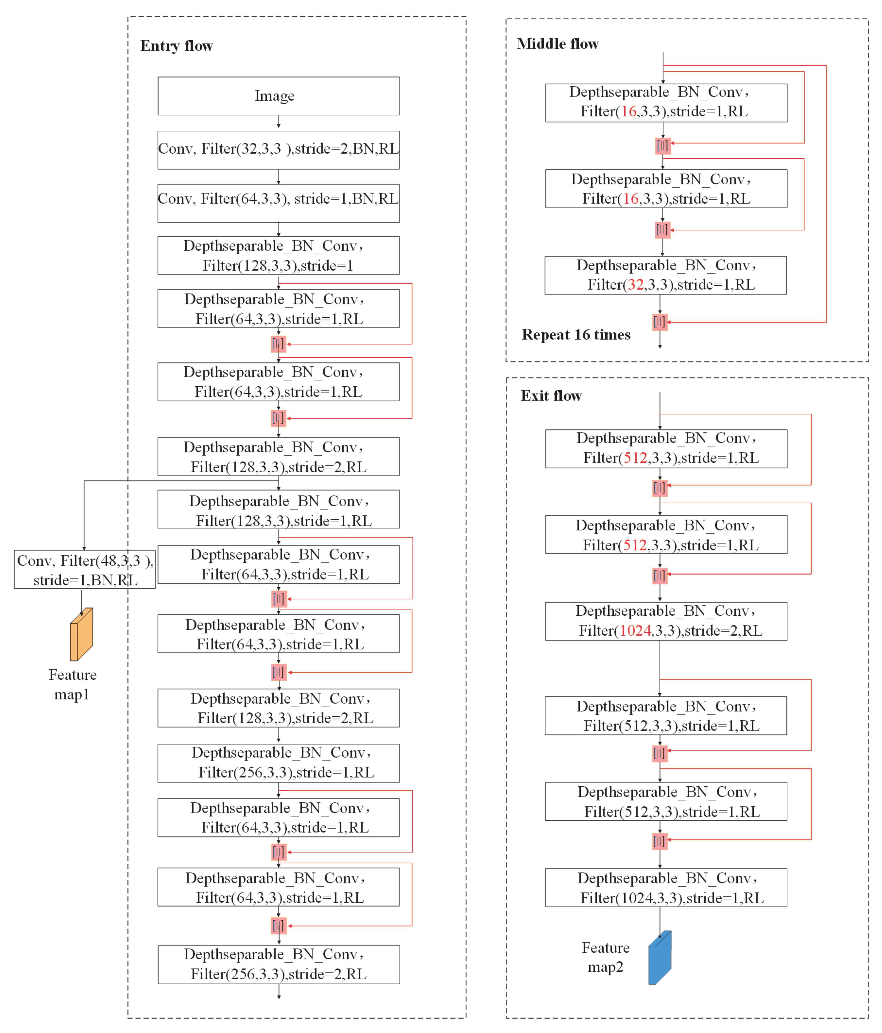
Although many neural networks, as we mentioned above, have been used for the semantic segmentation of RSI, it is difficult to extract a building with irregular shape or small size. The reasons can be distilled to the following: firstly, the current neural network mostly uses the skip-layer [25] to fuse deep features and shallow features. This method cannot fuse features between skip-layers sufficiently. Some neural networks also use the residual network connection method to merge deep features and shallow features, but in the residual block still lacks feature fusion; secondly, to control the number of parameters, most of the networks only extract the multi-scale features of pixels in the decoding stage and lacks the extraction of multi-scale features in the encoding stage. To fill the mentioned-above knowledges, a dense residual neural network (DR-Net) was therefore proposed by this paper, in which a deeplabv3+Net encoder/decoder backbone was employed by integrating densely connected DCNN with ResNet. To reduce the complexity of the network, we decreased the number of parameters by reducing the number of convolution kernels in the network.

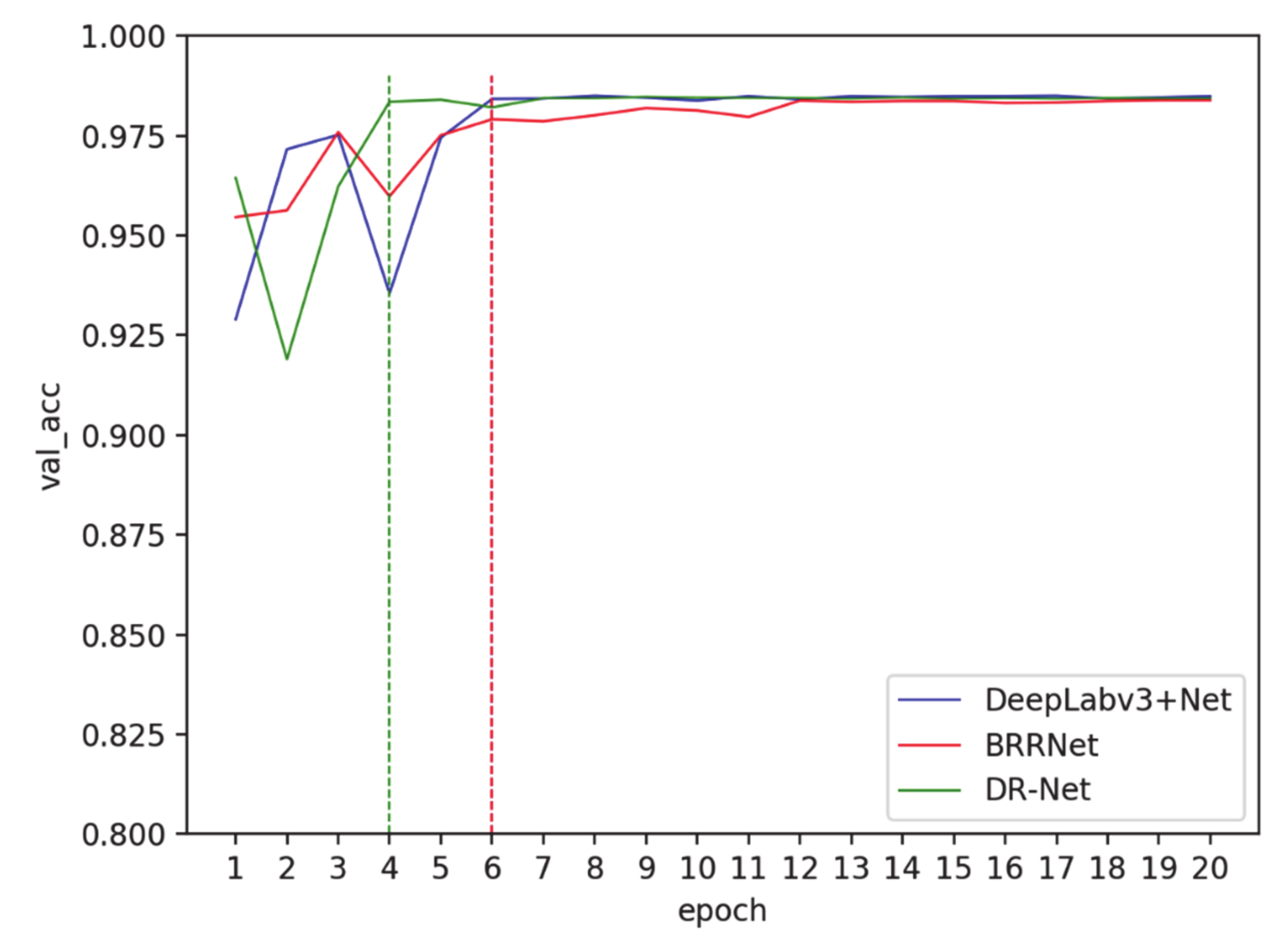
The highlights of this paper can be summarized as three aspects. Firstly, a dense residual neural network (DR-Net) was proposed, which uses a deeplabv3+Net encoder/decoder backbone, in combination with densely connected convolution neural network (DCNN) and residual network (ResNet) structure. Secondly, the number of parameters in this network is greatly reduced, but DR-Net still showed an outstanding performance in building extraction task. Thirdly, DR-Net has a faster convergence speed and consume less time to train.

The following section present the materials and the proposed network DR-Net. Section 3 explains the experiment and result in detail. In Section 4, we discuss the reasons why the DR-Net can perform well and give some directions to further improve its performance. Finally, in Section 5, conclusions about this paper are given.

2. Materials and Methods

2.1. Data

The WHU building data set [38] is often used to extract buildings from RSI. This data set not only contains aerial images, but also contains satellite images covering $1000{\mathrm{km}}^2$; at the same time, its label also contains raster and vectors. The aerial image (including 18,7000 buildings) covering in Christchurch, New Zealand, was downsampled to a ground resolution of 0.3 m and cropped into 8189 tiles of 512×512 pixels. These tiles were divided into three parts: the training set including 4736 tiles (130,500 buildings), the validation set including 1036 tiles (14,500 buildings), and the test set including 2416 tiles (42,000 buildings). We use these 0.3 m spatial resolution tiles as experimental data. In training process image tiles and response labels are put into the network; in testing process, only image tiles are put into the network. The area of the experiment data set is shown in Figure 1.

2.2. Densely Connected Neural Network

In order to further improve fusion of deep and shallow features in the neural network, a densely connected network (DCNN) was proposed [9]. In DCNN, the layer of neural network takes the outputs of each layer before it as inputs. That is, the input of the $l$-th layer is the output of the first to $\left(l-1\right)$th layer, and the expression is defined as: $x_l= H_l\left(\left[x_0, x_1, \dots x_{l-1}\right]\right)$. In the formula $\left[x_0, x_1, \dots x_{l-1}\right]$ indicates that the output feature maps of the 0-th to $\left(l-1\right)$th layer are concatenated in the channel dimension.

2.3. Residual Neural Network

As for the traditional convolutional neural network, in the process of forward propagation, the output $x_l$ of the $l$th layer is used as the input of the $\left(\mathrm{l}+1\right)$th layer of neural network. The expression is defined as: $x_l= H_l\left(x_{l-1}\right)$. The residual neural network (ResNet) [39] adds a skip connection on the basis of the conventional convolutional neural network, by passing the nonlinear transformation and identity function, and the expression is defined as: $x_l= H_l\left(x_{l-1}\right)+x_{l-1}$. One of advantages of ResNet is that the gradient can flow directly from a deep layer to a shallow layer, which can prevent the gradient disappearance and gradient explosion problems. However, compared with the feature map concatenated in the channel dimension, it will reduce the information contained in the feature map. Therefore, in this article, a DCNN structure is adopted in a residual neural network. At the same time, it concatenates the feature maps in the channel dimension instead of adding feature maps in the channel dimension.

2.4. Dense Residual Neural Network

This section mainly introduces the basic structure of the dense residual neural network (DR-Net). Inspired by DeepLabv3+Net [7] and DCCN [9], we proposed the DR-Net using deeplabv3+Net as backbone, in combination with the DCCN network and ResNet. The skeleton of deeplabv3+Net [7] is shown in Figure 2, which consists of an encoding and decoding module. The function of the encoding module is to extract the features of the input image step by step or layer by layer. With the stack of layers, feature maps extracted by deep layers become more abstract and contain richer semantic information which is helpful to the category of pixels. However, the spatial resolution of the feature maps becomes lower, because of the stride of convolution. This means that the feature map loses local information, such as boundaries and other details. Therefore, it is necessary to add a decoding module. The decoding module fuses the high spatial resolution feature map output by the shallow layers of the encoding module and the low spatial resolution feature maps output by the deep layers of decoding module to obtain a new feature map. This new feature map not only retains the semantic information that is conducive to classification, but also contains the spatial location characteristics which are more sensitive to details such as the boundary and shape of the buildings.

Compared with DeepLabV3+Net, the modified xception is replaced by the Dense xception module((DXM)) in DR-Net. DCCN and ResNet are introduced into the DXM which promotes the fusion of deep and shallow features In the Figure 3, structure of DXM is shown. conv represents the convolution operation; Filter() represents the convolution kernel, the numbers in parentheses represent the number of convolution kernels, the width and height of the convolution kernel; depthseparable_BN_Conv represents the depth separable convolution and batch normalization processing; stride represents the moving stride of the convolution kernel; RL represents the relu activation function, and [||] represents the splicing operation of feature maps in the channel dimension. In the entry flow, we adopt densely connected layers, which reduce the number of parameters and contribute to extract abstract features in shallow layers. We believe that, in deeper layers, abstract feature and detail features should be focused on at the same time. This is because in the deeper layers, the size of feature map is smaller, which could consume less memory of the computer. Thus, in middle flow, we adopted densely connected layers and modified residual layers. We connect feature maps in channel dimension instead of adding them together directly. In exit flow, similarly, modify as the entry flow is carried out.

2.5. Loss Function

Cross-entropy loss function [40], focal loss [41], and loss function based on dice coefficient [27,42,43,44] are commonly used in image semantic segmentation tasks. It has been proven that loss function based on dice coefficient performs better than Cross entropy loss function [45]. In order to test the performance of DR-Net with different loss functions, cross-entropy loss and dice loss were used with the DR-Net, respectively. The expressions of the cross-entropy loss function and the dice coefficient loss function [27] are shown in Functions (1)–(4):

$$T\left(p_{iK},l_{iK}\right)=\frac{{{\displaystyle \sum }}_{K=1}^{N_{class}}{w}_K{{\displaystyle \sum }}_{i=1}^{N_{pixels}}{p}_{iK}{l}_{iK}}{{{\displaystyle \sum }}_{K=1}^{N_{class}}{w}_K{{\displaystyle \sum }}_{K=1}^{N_{pixels}}\left(p_{iK}^2+l_{iK}^2-p_{iK}{l}_{iK}\right)}$$

(1)

$$\tilde{T}\left(p_{iK},l_{iK}\right)=T\left(p_{iK},l_{iK}\right)+T\left(1-p_{iK},1-l_{iK}\right)$$

(2)

$$diceloss=1-\tilde{T}\left(p_{iK},l_{iK}\right)$$

(3)

$$celoss=-\frac{1}{N_{pixels}}{{\displaystyle \sum }}_{i=1}^{N_{pixels}}{{\displaystyle \sum }}_{K=1}^{N_{class}}{l}_{iK}log\left(p_{iK}\right)$$

(4)

where $N_{class}$ represents the number of categories, in this paper $K=2$; $N_{pixels}$ represents the number of pixels in the image; $w_K$ represents the weight of the Kth pixel in the sample. The calculation formula is $w_K=v_K^{-2}$, where $v_K$ represents the Kth image in the sample. The number of elements; $p_{iK}$ represents the probability that the $i$th pixel in the image is predicted to be the k-th category; $l_{iK}$ represents the probability that the $i$th pixel in the image label belongs to the $k$-th category.

2.6. Evaluation Metrics

We adopted four evaluation metrics to measure the effectiveness of DR-Net: Intersection over Union (IoU), precision, recall, and $\mathrm{F}{1}_{\mathrm{Score}}$. IoU is commonly used to evaluate image semantic segmentation result by measuring the similarity between the predicted result and the ground truth. IoU is calculated as Function (5):

$$IoU=\frac{TP}{FN+TP+FP}$$

(5)

Accuracy refers to the proportion of positive samples that are predicted as positive samples among all the samples predicted as positive. The calculation of precision is shown in Function (6). Recall is the proportion of positive samples predicted to positive samples among all true positive samples. The calculation of recall is shown in Function (7).$\mathrm{F}{1}_{\mathrm{Score}}$ comprehensively take into account precision and recall. The calculation of $\mathrm{F}{1}_{\mathrm{Score}}$ is shown in Function (8).

$$Precision=\frac{TP}{TP+FP}$$

(6)

$$recall=\frac{TP}{TP+FN}$$

(7)

$$F{1}_{Score}=\frac{2\times Precision\times Rceall}{Precision+Rceall}$$

(8)

where TP refers to the number of positive samples (buildings) predicted to be positive samples. FP refers to the number of negative samples (backgrounds) that are predicted to be positive samples. TN refers to the number of negative samples that are predicted to be negative samples. FN refers to the number of positive samples that are predicted to be negative samples.

3. Experiments and Results

In this section, the experimental setting and experimental result will be presented. The experiments were divided into two parts. The first part was to test the performance of DR-net with different loss function. The second part was to evaluate the performance of different networks.

3.1. Experiment Setting

Due to the limitation of our computer memory, the batch size is set to 1. Before training, parameters in the network were initialized according to the normal distribution whose mean and standard deviation were set to 0.1 and 0.05, respectively. The initial learning rate was set to 0.001. The ADM method [44] was used as the optimization algorithm. During the training process, if the test error did not decrease in two consecutive epochs, the learning rate will be updated to 0.1 times, and then continue to train the network.

The DR-Net was set up based on TensorFlow 1.14 and keras 2.2.5. The computer’s operating system was win10, the computer’s configuration mainly included a CPU (i7-7700hq, 8G memory) and GPU (NVIDIA GeForce GTX1060, Max-Q design, 6GB memory).

3.2. Comparison of Different Loss Functions

In order to verify the performance of the DR-net with different loss functions, we conducted an experiment on cross-entropy loss and dice loss. The experimental protocol was described in Section 3.1. The trained DR-Net based on different loss functions were used to extract buildings from the test set, and the results and visualization were shown in

Table 1. Accuracy of DR-Net with different loss functions.

Methods	Recall	Precision	IoU	$\mathbf{F}{1}_{\mathbf{S}\mathbf{c}\mathbf{o}\mathbf{r}\mathbf{e}}$
DR-Net and celoss	0.907	0.943	0.860	0.925
DR-Net and dice loss	0.922	0.927	0.860	0.925

and Figure 4. In the visualization (including Figure 4, Figure 5 and Figure 6), the green depicts the buildings predicted correctly, the red shows buildings predicted to background, and the blue shows the background predicted to buildings. We found that, as far as IoU and F1 score were concerned, DR-Net with cross-entropy loss and dice loss had similar overall performance. But the DR-Net with cross-entropy loss has a higher recall and lower precision value than the DR-Net with dice loss. Thus, the dice loss can balance the relationship between recall and accuracy, while the binary cross-entropy cannot.

3.3. Comparison of Different Networks

Comparative accuracy of different network. It has been proven that the performance of BRRNet is better than PSPNet and Dilated ResNet50, RefineNet (ResNet50), Bayesian-SegNet in building extraction from RSI [31]. The deeplabv3+Net achieved good results in computer vision. So, we took deeplabv3+Net as a baseline, and analyzed the performances of deeplabv3+Net, BRRNet, and DR-Net with dice loss. The experimental details were set as described in Section 3.1. The performances of the three networks on the test set were shown in

Table 2. The performance of different methods.

Methods	Batch size	Recall	Precision	IoU	$\mathbf{F}{1}_{\mathbf{S}\mathbf{c}\mathbf{o}\mathbf{r}\mathbf{e}}$
BRRNet	1	0.913	0.935	0.859	0.924
Deeplbv3+Net	1	0.911	0.923	0.858	0.923
DR-Net	1	0.922	0.927	0.860	0.925

and Figure 5. The DR-Net for building extraction is slightly better than Deeplbv3+Net (with IoU/$\mathrm{F}{1}_{\mathrm{Score}}$ increased by 0.002/0.002) and BRRNet (with IoU/$\mathrm{F}{1}_{\mathrm{Score}}$ increased by 0.001/0.001). Thus, compared with BRRNet and deepLabv3+ net, the Overall performance of DR-Net slightly improved.

Comparative complexity of different networks. With the increasing number of layers, the feature map contains more semantic information, and there are more parameters that need to be trained. The number of parameters is an important indicator for evaluating the efficiency of a network. The more parameters, the more memories are needed during the training and testing process. It is meaningful to talk about the number of parameters in the networks. Based on this consideration, we analyzed the number parameters in the three networks, and the result was shown in

Table 3. The complexity of different networks. Row “Total parameters” represents the total parameters in a module; Row “Time” represents the time consumed in every training epoch; Row “epochs” represents the number of training epochs when acquire the best trained module.

	Deeplabv3+Net	DR-Net	BRRNet
Total params (million)	41	9	17
Time (min/epoch)	45	37	68
Epochs	11	9	12

. The DR-Net with 9 million parameters, Deeplabv3+Net with 41million parameters, and BRRNet with 17 million parameters show that DR-Net contains far fewer parameters than deeplabv3+Net and BRRNet. So, DR-Net needs less memory in training and test processing. Row “Time” in Table 3 shows that, compared with Deeplabv3+Net and BRRNet, the DR-Net reduced 8 minutes and 28 minutes, respectively, in every training epoch. Row “Epoch” in Table 3 shows that, the DR-Net could be trained well through 9 training epochs, while Deeplabv3+Net needs 11 and BRRNet need 12 training epochs to obtain the best trained models.

Based on the comparative analysis of the number parameters in different networks, we try to increase the batch size during the training process and further analyzed the effects of different networks. We found that, in terms of Deeplabv3+ and BRRNet, when set batch size to 2, it will exceed the memory range of the GPU; while for DR-Net, it will not exceed the storage range. This situation further proved that the complexity of DR-Net is better than Deeplabv3+Net and BRRNet. In order to analyze the effects of different networks under the limited computing resources, according to the experimental setting described in Section 3.1, we set the batch-size to 2, training DR-Net, and its performance is shown in

Table 4. The performance of DR-Net with dice loss (in the training process, the batch size was set to 2).

Method	Batch size	Recall	Precision	IoU	$\mathbf{F}{1}_{\mathbf{S}\mathbf{c}\mathbf{o}\mathbf{r}\mathbf{e}}$
DR-Net and dice loss	2	0.933	0.943	0.883	0.938

and Figure 6. Comparing Table 2 and Table 4 we found that the DR-Net for building extraction is significantly better than Deeplbv3+Net (with IoU/$\mathrm{F}{1}_{\mathrm{Score}}$ increased by 0.025/0.015) and BRRNet (with IoU/$\mathrm{F}{1}_{\mathrm{Score}}$ increased by 0.024/0.014). Figure 5 and Figure 6 showed that DR-Net improve the performance in extracting buildings with small size and irregular shape. As such, the DR-Net does not scarify its capability to reduce the number of parameters. We agreed that the structure of DR-Net plays a key role in improving its performance. To further demonstrate the effects of the networks, Appendix A shows the performance of different networks on test areas (including test A and test B).

Comparative convergence speed of different network. The convergence of a network means that the loss function value floats in a small range during the training process. The learning ability of the network can be understood as the ability to extract useful features. The learning rate reduced means that the neural network structure cannot learn useful features to improve its performance at the current learning rate. It must update the parameters with a smaller step (learning rate) to extract more refined features. We can judge whether the learning rate is convenient to extract useful features via evaluate whether the accuracy is still increased under this learning rate. Therefore, we use the number of training epoch and the accuracy when the learning rate is first reduced as an index to describe the learning ability of the neural network.

We analyzed the convergence speed and learning ability of the neural network, and the results are shown in Figure 7. During the training process, the learning rate of DR-Net decreased at the fourth epoch. At this time, the accuracy of the verification set was 0.984. The learning rate of DeepLabv3+Net was first reduced at the sixth epoch, with the accuracy rate 0.984. The learning rate of BRRNet also first dropped at the sixth epoch with the accuracy rate 0.979. We found that When the learning rate dropped at the first time, the accuracy gap of the three networks was within 0.005, but the number of training epoch had a wider gap. We can conclude that, as for accuracy, three network structures basically have the same performance, but the DR-Net has a faster convergence speed.

Comparative generalization ability of different networks. Generalization ability is used to measure a module trained based on a data set, whether would perform well on another data set. To further verify the generalization of different networks, we trained three modules on WHU data set, and tested these three modules on Massachusetts Building Dataset [20]. This dataset contains 151 aerial images of the Boston area. The size of each image is 1500 × 1500 pixels with the resolution of 1 m, and the testing set has 10 images. Thus, the Massachusetts Building Dataset and WHU data set covering different regions consist of images with different spatial resolutions.

Table 5. The transfer learning of different methods (networks were trained on the WHU data set). The column “Massachusetts” represents the results of the networks that were trained on the training set of the Massachusetts Building Dataset and then tested on the test set of the Massachusetts Building Dataset. The column "WHU set" represents the results of the networks that were trained on the training set of the Massachusetts Building Dataset, and then tested on the test set of the WHU data set.

Methods	Batch Size	WHU Data		Massachusetts
		IoU	$\mathbf{F}{1}_{\mathbf{S}\mathbf{c}\mathbf{o}\mathbf{r}\mathbf{e}}$	IoU	$\mathbf{F}{1}_{\mathbf{S}\mathbf{c}\mathbf{o}\mathbf{r}\mathbf{e}}$
BRRNet and dice loss	1	0.859	0.924	0.116	0.208
Deeplabv3+Net and dice loss	1	0.858	0.923	0.202	0.336
DR-Net and dice loss	1	0.860	0.925	0.112	0.201
DR-Net and dice loss	2	0.883	0.938	0.101	0.184

and

Table 6. The transfer learning of different methods (networks were trained on the Massachusetts Building Dataset). The column “Massachusetts” represents the results of the networks that were trained on the training set of the Massachusetts Building Dataset and then tested on the test set of the Massachusetts Building Dataset. The column "WHU set" represents the results of the networks that were trained on the training set of the Massachusetts Building Dataset, and then tested on the test set of WHU data set.

Methods	Batch Size	Massachusetts		WHU Set
		IoU	$\mathbf{F}{1}_{\mathbf{S}\mathbf{c}\mathbf{o}\mathbf{r}\mathbf{e}}$	IoU	$\mathbf{F}{1}_{\mathbf{S}\mathbf{c}\mathbf{o}\mathbf{r}\mathbf{e}}$
BRRNet and dice loss	1	0.579	0.733	0.401	0.572
Deeplabv3+Net and dice loss	1	0.614	0.761	0.389	0.561
DR-Net and dice loss	1	0.630	0.773	0.279	0.437
DR-Net and dice loss	2	0.660	0.795	0.288	0.447

show the test results of different networks trained and tested based on different data sets. BRRNet and Deeplabv3+Net had better generalization abilities. We think this is because, during the training process, DR-Net better fused shallow and deep features, while these fused features could not transfer to other data sets.

Comparing the column “WHU data” in Table 5 and column “Massachusetts” in Table 6 we found DR-Net had the best performance among three networks, but all methods obtained a better result in the WHU data set. Comparing Table 5 and Table 6, any network among the three methods had a better performance when trained and tested on the WHU building data set.

4. Discussion

This paper proposes a new convolutional neural network structure named DR-Net for extracting buildings from heigh resolution RSI. DR-Net uses deeplabv3+Net as a backbone and combines the modules of DCNN with ResNet, so that the network can not only better extract the context information from RSI but also greatly reduce the number of parameters.

The DR-Net can achieve better performance in extracting buildings. We consider that each layer of the DR-Net contains the more original spectral information in the image. This spectral information can better preserve boundaries between buildings and background. The input of each layer within DR-Net contains the output of all layers before the current layer. This structure makes each layer contains the information about shallow features and the abstract features obtained in deeper layers. In fact, it is similar to concatenate the original RSI and the abstract features together in channel dimension. With the increasing of depth, the proportion of original information input into each layer is decreased, but does not disappear. We believe that this design can better integrate contextual information contained in shallow and deep feature maps. Therefore, DR-Net can achieve better results in the extraction of buildings.

Compared with the deeplabv3+ neural network, DR-Net reduces the number of parameters by dropping off the number of convolution kernels, and make the network more lightweight, easier to train. More importantly, DR-Net does not sacrifice its performance. Although, when batch size is set to 1, three networks have similar performance, but thinking about the numbers of parameters and the complexity of networks, it could conclude that DR-Net has made a great progress. Moreover, under the same hardware configuration (as described in Section 3.1), batch size can be set to 2 in DR-Net. As a comparation, if batch size is set to 2 in deeplabv3+Net and BRRNet, the nets cannot be trained, because of the limitation of the GPU.

When the computer’s computing performance and memory of GPU are limited, try to reduce the number of convolution kernels in the neural network, and increase batch sizes; this may improve the performance of the network. We have not done further research and discussion on the balance between the number of convolution kernels and batch size in a neural network. This work will be carried out in the future.

It is important to note that this paper focuses on improving the performance of DR-Net. We considered that, only in a same situation where the data set, the memory and performance of computer should remain the same, the performance of different neural networks can be measured. Thus, in this article, we did not use data enhancement strategies. Some results of other articles [30,38] may be better than ours, but we found that their GPU memory is 11G and 12G, respectively, about 2 times ours. At the same time, some data enhanced strategies were adopted in these paper [30,38]. Thus, we thought that our result and articles [30,38] were not based on the same foundation, so we cannot simply judge which one is better or not.

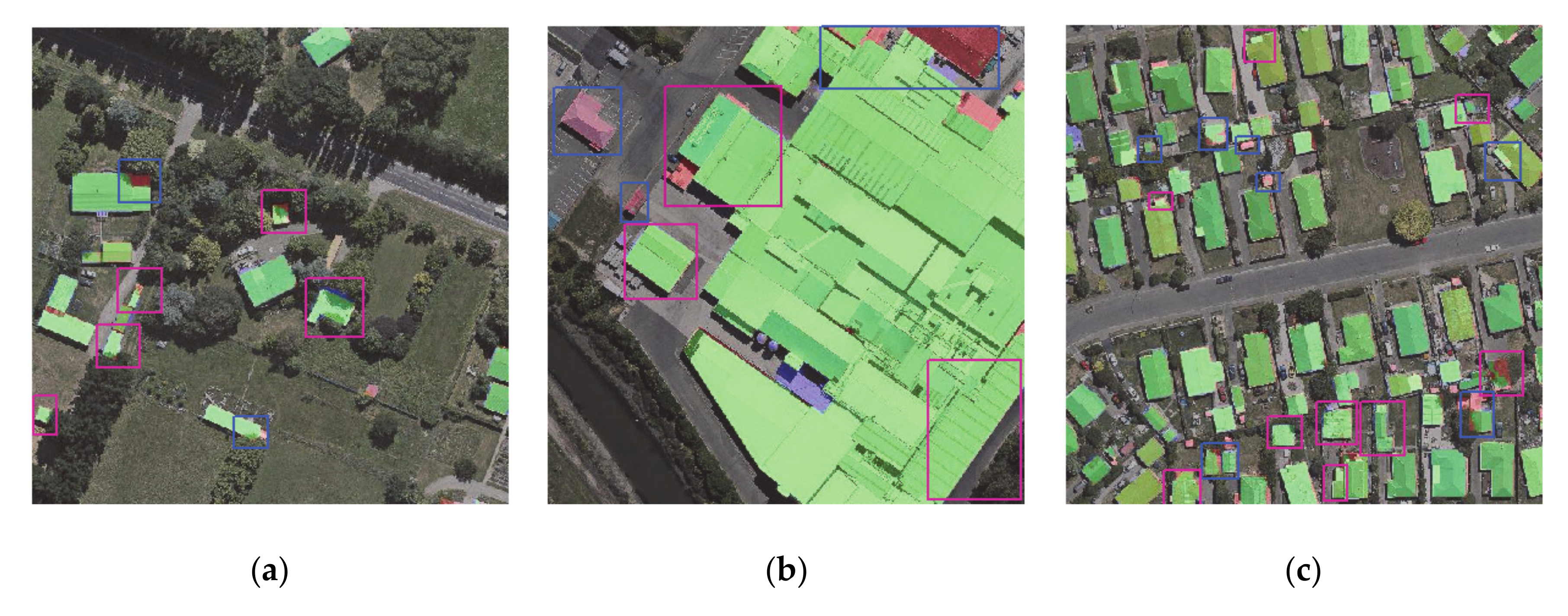
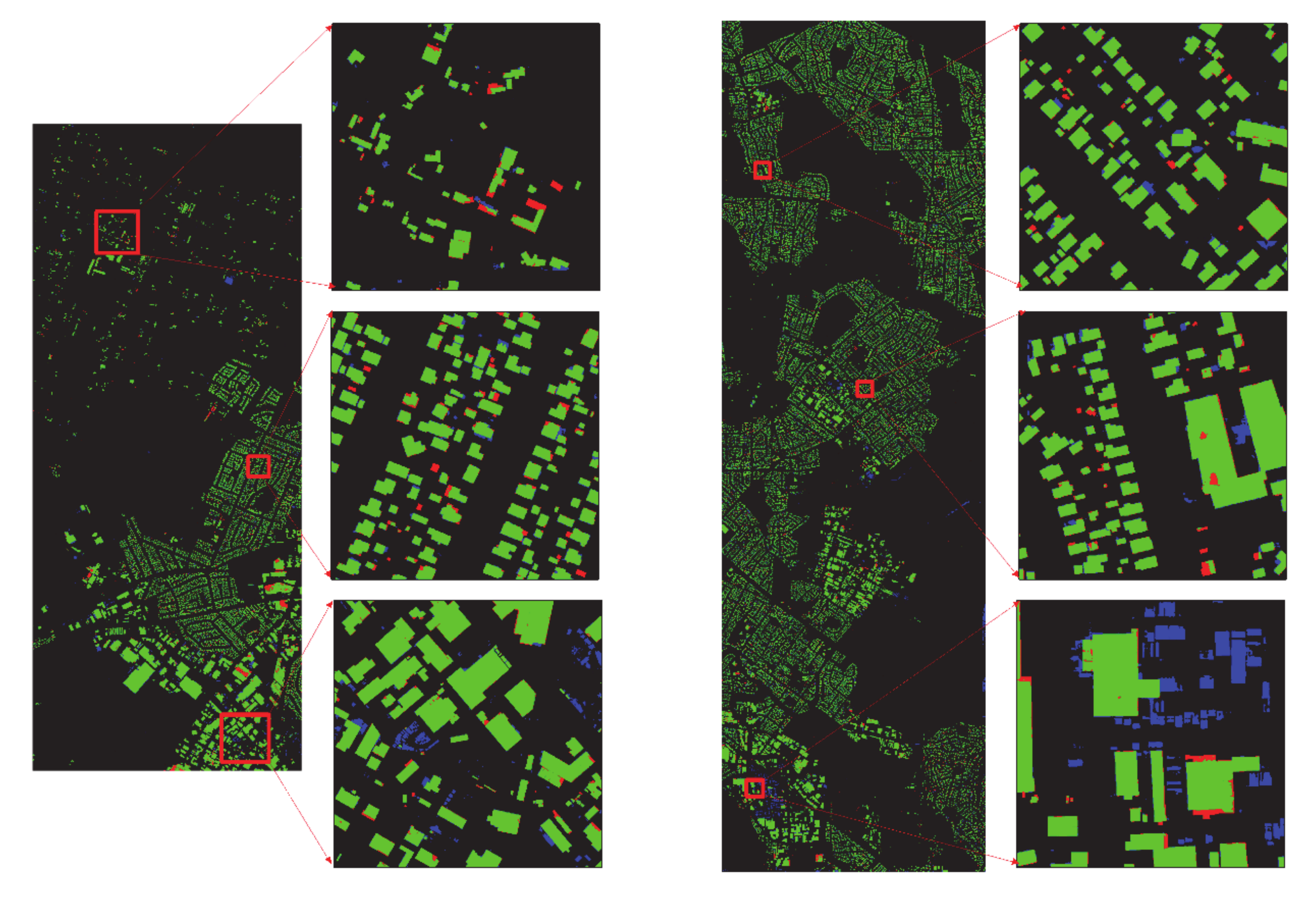
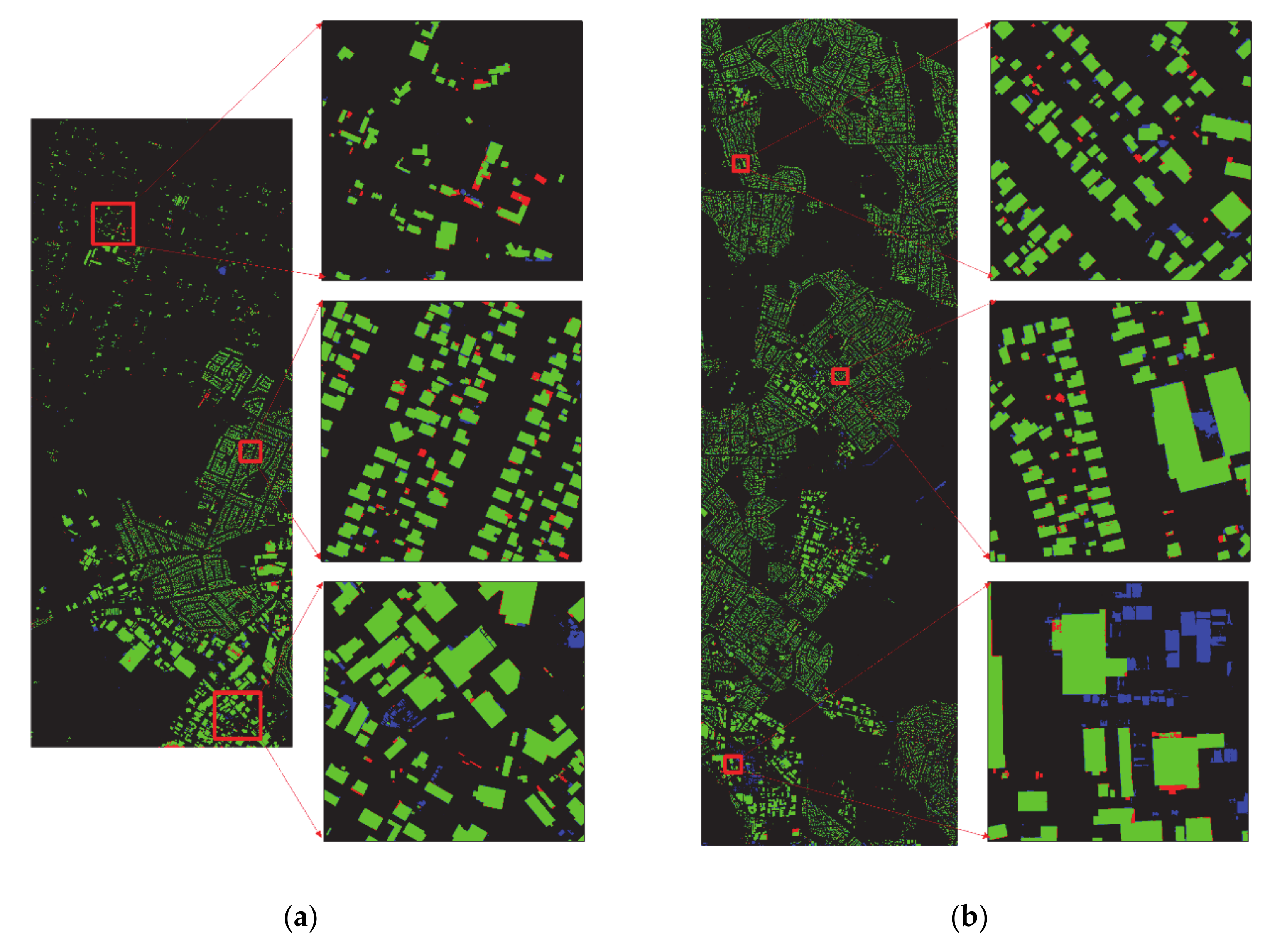
We investigated the wrong areas, where the buildings were predicted as backgrounds or backgrounds were predicted as buildings. We found some interesting phenomenon: Firstly, some background areas similar to buildings were predicted to buildings, such as some containers were regarded as buildings. In fact, it is difficult for the naked eye to recognize containers from a 500x500 pixels image tile. Secondly, some buildings under construction were predicated as backgrounds, because these buildings had different contexture and spectrum response from already built buildings, at the same time, only a few of buildings under construction in the training data set.

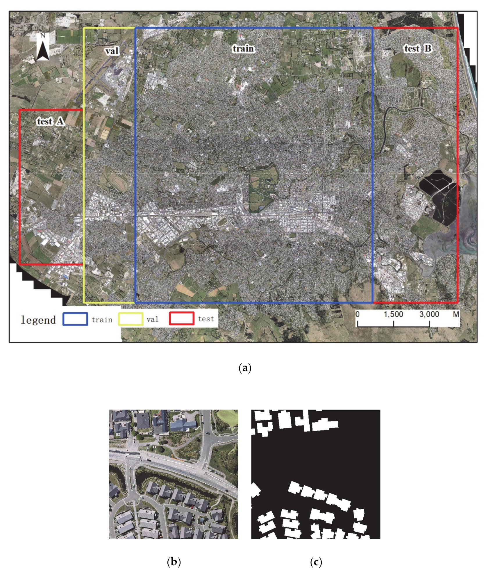
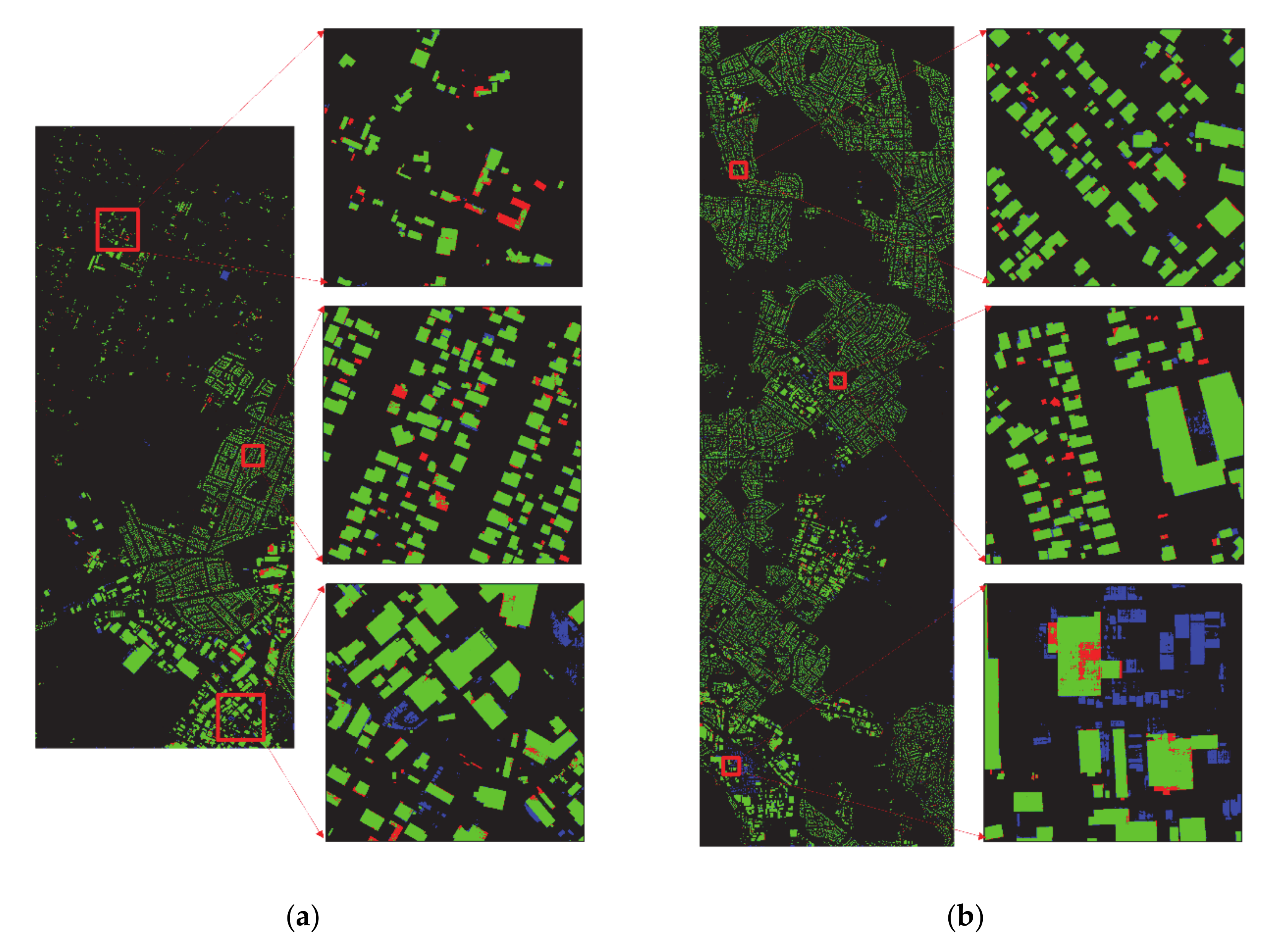
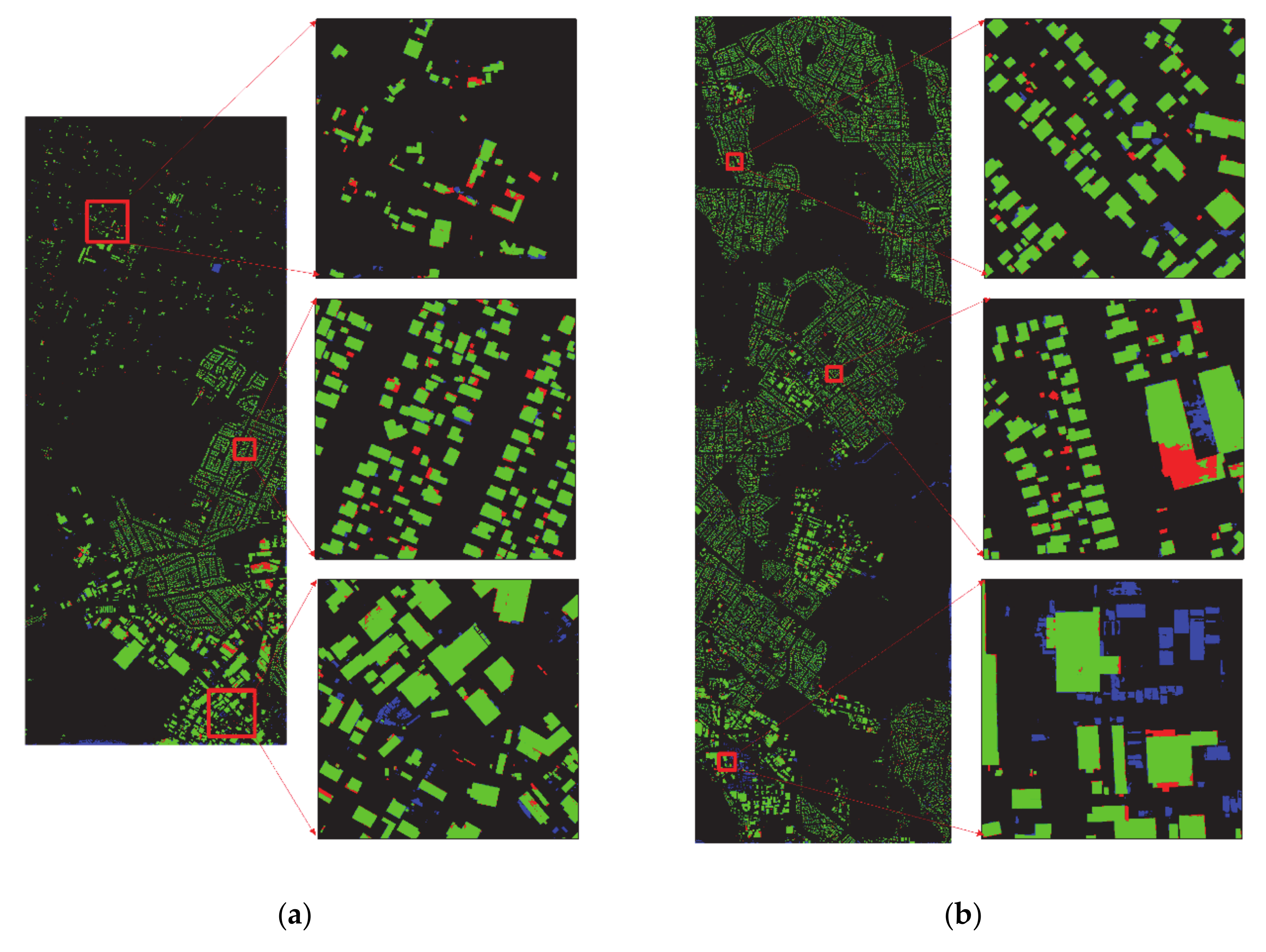
We found networks trained in Massachusetts and tested on WHU building data set had a better performance than networks trained on WHU building data set and tested on Massachusetts. We think this is because WHU building data set has higher spatial resolution than Massachusetts. Another interesting phenomenon is that BRRNet and Deeplabv3+Net had better generalization abilities. We think this is because during the training process, DR-Net could better fused shallow and deep feature, while these fused features cannot transfer to other datasets directly.

We give some possible directions to further improve the performance of DR-Net. The first is to introduce advanced feature extractor, such as Feature Pyramid Network (FPN) [46]. The second is to combine the multi-task learning mechanism and attention mechanism [47].

5. Conclusions

In this paper, we propose a new deep learning structure named DR-Net which is based on ResNet and DCNN, combining skeleton of deeplabv3+Net. The DR-Net has a similar performance based on celoss and dice loss, but the dice loss can balance the relationship between recall and accuracy, while the binary cross-entropy cannot. Compared with the benchmark networks, the DR-Net has two advantages. Firstly, it can fully integrate the features extracted by the shallow and deep layers of network, and improve the performance of extracting buildings from RSI, especially for buildings with small size and irregular shapes. Secondly, DR-Net has a faster convergence speed. Moreover, the number of parameters of the DR-Net is greatly reduced, and it occupies less memory during the training and testing process. Compared with other networks, DR-Net could achieve a better performance when CPU or GPU memory is limited. However, the experiment on the generalization ability of different networks showed that the generalization ability of DR-Net needs improvement.

References

1. Blaschke, T. Object based image analysis for remote sensing. J. Photogramm. Remote Sens. 2010, 65, 2–16. [Google Scholar] [CrossRef] [Green Version]
2. Ronneberger, O.; Fischer, P.; Brox, T. U-net: Convolutional networks for biomedical image segmentation. In Proceedings of the International Conference on Medical image computing and computer-assisted intervention, Munich, Germany, 5–9 October 2015; pp. 234–241. [Google Scholar]
3. Badrinarayanan, V.; Kendall, A.; Cipolla, R. Segnet: A deep convolutional encoder-decoder architecture for image segmentation. IEEE Trans. Pattern Anal. Mach. Intell. 2017, 39, 2481–2495. [Google Scholar] [CrossRef] [PubMed]
4. Chen, L.-C.; Papandreou, G.; Kokkinos, I.; Murphy, K.; Yuille, A.L. Deeplab: Semantic image segmentation with deep convolutional nets, atrous convolution, and fully connected crfs. IEEE Trans. Pattern Anal. Mach. Intell. 2017, 40, 834–848. [Google Scholar] [CrossRef] [PubMed]
5. Chollet, F. Xception: Deep Learning with Depthwise Separable Convolutions. In Proceedings of the 30th IEEE Conference on Computer Vision and Pattern Recognition, Honolulu, HI, USA, 21–26 July 2017; pp. 1800–1807. [Google Scholar]
6. Chen, L.-C.; Papandreou, G.; Schroff, F.; Adam, H. Rethinking atrous convolution for semantic image segmentation. arXiv 2017, arXiv:1706.05587. [Google Scholar]
7. Chen, L.-C.; Papandreou, G.; Schroff, F.; Adam, H. Encoder-Decoder with Atrous Separable Convolution for Semantic Image Segmentation. In Proceedings of the European Conference on Computer Vision (ECCV), Munich, Germany, 8–14 September 2018; pp. 801–818. [Google Scholar]
8. Liu, W.; Rabinovich, A.; Berg, A.C. Parsenet: Looking wider to see better. arXiv 2015, arXiv:1506.04579. [Google Scholar]
9. Huang, G.; Liu, Z.; Van Der Maaten, L.; Weinberger, K.Q. Densely connected convolutional networks. In Proceedings of the IEEE Conference on Computer Vision and Pattern Recognition, Honolulu, HI, USA, 21–26 July 2017; pp. 4700–4708. [Google Scholar]
10. Papandreou, G.; Kokkinos, I.; Savalle, P.-A. Modeling Local and Global Deformations in Deep Learning: Epitomic Convolution, Multiple Instance Learning, and Sliding Window Detection. In Proceedings of the IEEE Conference on Computer Vision and Pattern Recognition, Boston, MA, USA, 7–12 June 2015; pp. 390–399. [Google Scholar]
11. Dai, J.F.; Li, Y.; He, K.M.; Sun, J. R-fcn: Object detection via region-based fully convolutional networks. arXiv 2016, arXiv:1605.06409. [Google Scholar]
12. Ioffe, S.; Szegedy, C. Batch normalization: Accelerating deep network training by reducing internal covariate shift. arXiv 2015, arXiv:1502.03167. [Google Scholar]
13. Grauman, K.; Darrell, T. The pyramid match kernel: Discriminative classification with sets of image features. In Proceedings of the Tenth IEEE International Conference on Computer Vision (ICCV’05), Beijing, China, 17–21 October 2005; pp. 1458–1465. [Google Scholar]
14. Lazebnik, S.; Schmid, C.; Ponce, J. Beyond bags of features: Spatial pyramid matching for recognizing natural scene categories. In Proceedings of the 2006 IEEE Computer Society Conference on Computer Vision and Pattern Recognition (CVPR’06), New York, NY, USA, 17–22 June 2006; pp. 2169–2178. [Google Scholar]
15. He, K.; Zhang, X.; Ren, S.; Sun, J. Spatial pyramid pooling in deep convolutional networks for visual recognition. IEEE Trans. Pattern Anal. Mach. Intell. 2015, 37, 1904–1916. [Google Scholar] [CrossRef] [Green Version]
16. LeCun, Y.; Boser, B.; Denker, J.S.; Henderson, D.; Howard, R.E.; Hubbard, W.; Jackel, L.D. Backpropagation applied to handwritten zip code recognition. Neural Comput. 1989, 1, 541–551. [Google Scholar] [CrossRef]
17. Rawat, W.; Wang, Z.H. Deep convolutional neural networks for image classification: A comprehensive review. Neural Comput. 2017, 29, 2352–2449. [Google Scholar] [CrossRef]
18. Ball, J.; Anderson, D.; Chan, C.S. Comprehensive survey of deep learning in remote sensing: Theories, tools, and challenges for the community. J. Appl. Remote Sens. 2017, 11, 042609. [Google Scholar] [CrossRef] [Green Version]
19. Farabet, C.; Couprie, C.; Najman, L.; LeCun, Y. Learning hierarchical features for scene labeling. IEEE Trans. Pattern Anal. Mach. Intell. 2013, 35, 1915–1929. [Google Scholar] [CrossRef] [PubMed] [Green Version]
20. Mnih, V. Machine Learning for Aerial Image Labeling. Ph.D. Thesis, University of Toronto, Toronto, ON, Canada, 2013. [Google Scholar]
21. Girshick, R.; Donahue, J.; Darrell, T.; Malik, J. Rich feature hierarchies for accurate object detection and semantic segmentation. In Proceedings of the 2014 IEEE Conference on Computer Vision and Pattern Recognition, New York, NY, USA, 23–28 June 2014; pp. 580–587. [Google Scholar]
22. Gupta, S.; Girshick, R.; Arbelaez, P.; Malik, J. Learning rich features from rgb-d images for object detection and segmentation. In Proceedings of the 13th European Conference on Computer Vision (ECCV), Zurich, Switzerland, 6–12 September 2014; Fleet, D., Pajdla, T., Schiele, B., Tuytelaars, T., Eds.; Springer: Zurich, Switzerland; pp. 345–360. [Google Scholar]
23. Zhang, C.; Sargent, I.; Pan, X.; Li, H.; Gardiner, A.; Hare, J.; Atkinson, P.M. An object-based convolutional neural network (ocnn) for urban land use classification. Remote Sens. Environ. 2018, 216, 57–70. [Google Scholar] [CrossRef] [Green Version]
24. Zhao, W.; Du, S.; Emery, W.J. Object-based convolutional neural network for high-resolution imagery classification. IEEE J. Sel. Top. Appl. Earth Observ. 2017, 10, 3386–3396. [Google Scholar] [CrossRef]
25. Shelhamer, E.; Long, J.; Darrell, T. Fully convolutional networks for semantic segmentation. IEEE Trans. Pattern Anal. Mach. Intell. 2017, 39, 640–651. [Google Scholar] [CrossRef] [PubMed]
26. Liu, P.; Liu, X.; Liu, M.; Shi, Q.; Yang, J.; Xu, X.; Zhang, Y. Building footprint extraction from high-resolution images via spatial residual inception convolutional neural network. Remote Sens. 2019, 11, 830. [Google Scholar] [CrossRef] [Green Version]
27. Diakogiannis, F.I.; Waldner, F.; Caccetta, P.; Wu, C. Resunet-a: A deep learning framework for semantic segmentation of remotely sensed data. ISPRS J. Photogramm. Remote Sens. 2020, 162, 94–114. [Google Scholar] [CrossRef] [Green Version]
28. Ma, J.J.; Wu, L.L.; Tang, X.; Liu, F.; Zhang, X.R.; Jiao, L.C. Building extraction of aerial images by a global and multi-scale encoder-decoder network. Remote Sens. 2020, 12, 19. [Google Scholar] [CrossRef]
29. Liu, Y.H.; Gross, L.; Li, Z.Q.; Li, X.L.; Fan, X.W.; Qi, W.H. Automatic building extraction on high-resolution remote sensing imagery using deep convolutional encoder-decoder with spatial pyramid pooling. IEEE Access 2019, 7, 128774–128786. [Google Scholar] [CrossRef]
30. Liu, H.; Luo, J.; Huang, B.; Hu, X.; Sun, Y.; Yang, Y.; Xu, N.; Zhou, N. De-net: Deep encoding network for building extraction from high-resolution remote sensing imagery. Remote Sens. 2019, 11, 2380. [Google Scholar] [CrossRef] [Green Version]
31. Shao, Z.; Tang, P.; Wang, Z.; Saleem, N.; Yam, S.; Sommai, C. Brrnet: A fully convolutional neural network for automatic building extraction from high-resolution remote sensing images. Remote Sens. 2020, 12, 1050. [Google Scholar] [CrossRef] [Green Version]
32. Wei, S.; Ji, S.; Lu, M. Toward automatic building footprint delineation from aerial images using cnn and regularization. IEEE Trans. Geosci. Remote Sensing 2020, 58, 2178–2189. [Google Scholar] [CrossRef]
33. Liu, Y.H.; Zhou, J.; Qi, W.H.; Li, X.L.; Gross, L.; Shao, Q.; Zhao, Z.G.; Ni, L.; Fan, X.W.; Li, Z.Q. Arc-net: An efficient network for building extraction from high-resolution aerial images. IEEE Access 2020, 8, 154997–155010. [Google Scholar] [CrossRef]
34. Yi, Y.N.; Zhang, Z.J.; Zhang, W.C.; Zhang, C.R.; Li, W.D.; Zhao, T. Semantic segmentation of urban buildings from vhr remote sensing imagery using a deep convolutional neural network. Remote Sens. 2019, 11, 19. [Google Scholar] [CrossRef] [Green Version]
35. Ruder, S. An Overview of Multi-Task Learning in Deep Neural Networks. arXiv 2017, arXiv:1706.05098. [Google Scholar]
36. Ye, Z.; Fu, Y.; Gan, M.; Deng, J.; Comber, A.; Wang, K. Building extraction from very high resolution aerial imagery using joint attention deep neural network. Remote Sens. 2019, 11, 2970. [Google Scholar] [CrossRef] [Green Version]
37. Panboonyuen, T.; Jitkajornwanich, K.; Lawawirojwong, S.; Srestasathiern, P.; Vateekul, P. Semantic segmentation on remotely sensed images using an enhanced global convolutional network with channel attention and domain specific transfer learning. Remote Sens. 2019, 11, 83. [Google Scholar] [CrossRef] [Green Version]
38. Ji, S.P.; Wei, S.Q.; Lu, M. Fully convolutional networks for multisource building extraction from an open aerial and satellite imagery data set. IEEE Trans. Geosci. Remote Sensing 2019, 57, 574–586. [Google Scholar] [CrossRef]
39. He, K.; Zhang, X.; Ren, S.; Sun, J. Deep residual learning for image recognition. In Proceedings of the IEEE Conference on Computer Vision and Pattern Recognition (CVPR), Las Vegas, NV, USA, 27–30 June 2016; pp. 770–778. [Google Scholar]
40. De Boer, P.T.; Kroese, D.P.; Mannor, S.; Rubinstein, R.Y. A tutorial on the cross-entropy method. Ann. Oper. Res. 2005, 134, 19–67. [Google Scholar] [CrossRef]
41. Lin, T.Y.; Goyal, P.; Girshick, R.; He, K.M.; Dollar, P. Focal loss for dense object detection. IEEE Trans. Pattern Anal. Mach. Intell. 2020, 42, 318–327. [Google Scholar] [CrossRef] [Green Version]
42. Milletari, F.; Navab, N.; Ahmadi, S.A. V-net: Fully convolutional neural networks for volumetric medical image segmentation. In Proceedings of the 2016 Fourth International Conference on 3D Vision (3DV), Stanford, CA, USA, 25–28 October 2016; pp. 565–571. [Google Scholar]
43. Sudre, C.H.; Li, W.Q.; Vercauteren, T.; Ourselin, S.; Cardoso, M.J. Generalised Dice overlap as a deep learning loss function for highly unbalanced segmentations. arXiv 2017, arXiv:1707.03237. [Google Scholar]
44. Drozdzal, M.; Vorontsov, E.; Chartrand, G.; Kadoury, S.; Pal, C. The Importance of Skip Connections in Biomedical Image Segmentation. arXiv 2016, arXiv:1608.04117. [Google Scholar]
45. Novikov, A.A.; Lenis, D.; Major, D.; Hladuvka, J.; Wimmer, M.; Buhler, K. Fully convolutional architectures for multiclass segmentation in chest radiographs. IEEE Trans. Med. Imaging 2018, 37, 1865–1876. [Google Scholar] [CrossRef] [PubMed] [Green Version]
46. Lin, T.Y.; Dollar, P.; Girshick, R.; He, K.M.; Hariharan, B.; Belongie, S. Feature pyramid networks for object detection. In Proceedings of the 30th IEEE/CVF Conference on Computer Vision and Pattern Recognition (CVPR), Honolulu, HI, USA, 21–26 July 2017; pp. 936–944. [Google Scholar]
47. Takikawa, T.; Acuna, D.; Jampani, V.; Fidler, S. Gated-scnn: Gated shape cnns for semantic segmentation. In Proceedings of the IEEE International Conference on Computer Vision, Seoul, Korea, 27 October–2 November 2019; pp. 5229–5238. [Google Scholar]
Figure 1. The WHU building data set. (a) shows the region of the RSI covering. The training area is the blue box, valid area is in the yellow box and test areas are in red boxes (containing test A and test B). (b,c) show image tile and label with size 512 × 512 pixels, respectively.
Remotesensing 13 00294 g001
Figure 2. The basic structure of DR-Net which is modified from deeplabv3+Net.
Remotesensing 13 00294 g002
Figure 3. The structure of Dense xception module (DXM).
Remotesensing 13 00294 g003
Figure 4. The visualization of building extraction results based on different loss function. The first row (ac) shows the results of DR-Net based on the binary cross entropy loss, and the second row (df) shows the result of DR-Net based on the dice loss.
Remotesensing 13 00294 g004
Figure 5. The performance of different networks. In the first row, (ac) show the performance of BRRNet; In the second row, (df) show the performance of DeepLabv3+Net; In the third row, (gi) show the performance of DR-Net. Yellow boxes represent best performance among three methods; blue boxes represent a relative worse performance among three methods.
Remotesensing 13 00294 g005aRemotesensing 13 00294 g005b
Figure 6. The effects of DR-Net and the batch size was set to 2. (ac) show the performance of DR-Net. Pink boxes annotate the best performance area compared with other three methods whose performance is shown in Table 2 and Figure 5.
Remotesensing 13 00294 g006
Figure 7. The relationship between accuracy and the number of training epochs. The vertical dashed line in the figure represents the position where the learning rate drops for the first time. The learning rate of DeepLabv3+Net and BRRNet were first dropped at the sixth training epoch.
Remotesensing 13 00294 g007