
Multi-Block Mixed Sample Semi-Supervised Learning for SAR Target Recognition

1
College of Computer Science and Technology, Harbin Engineering University, Harbin 150001, China
2
Heilongjiang Hengxun Technology Co., Ltd., Harbin 150001, China
*
Author to whom correspondence should be addressed.
Remote Sens. 2021, 13(3), 361; https://0-doi-org.brum.beds.ac.uk/10.3390/rs13030361
Submission received: 31 December 2020
/
Revised: 19 January 2021
/
Accepted: 20 January 2021
/
Published: 21 January 2021
(This article belongs to the Special Issue Deep Learning for Radar and Sonar Image Processing)
Abstract
:In recent years, synthetic aperture radar (SAR) automatic target recognition has played a crucial role in multiple fields and has received widespread attention. Compared with optical image recognition with massive annotation data, lacking sufficient labeled images limits the performance of the SAR automatic target recognition (ATR) method based on deep learning. It is expensive and time-consuming to annotate the targets for SAR images, while it is difficult for unsupervised SAR target recognition to meet the actual needs. In this situation, we propose a semi-supervised sample mixing method for SAR target recognition, named multi-block mixed (MBM), which can effectively utilize the unlabeled samples. During the data preprocessing stage, a multi-block mixed method is used to interpolate a small part of the training image to generate new samples. Then, the new samples are used to improve the recognition accuracy of the model. To verify the effectiveness of the proposed method, experiments are carried out on the moving and stationary target acquisition and recognition (MSTAR) data set. The experimental results fully demonstrate that the proposed MBM semi-supervised learning method can effectively address the problem of annotation insufficiency in SAR data sets and can learn valuable information from unlabeled samples, thereby improving the recognition performance.
1. Introduction
Automatic target recognition (ATR) for SAR has been widely applied in mineral resource exploration, geographic information collection, and marine monitoring, due to its all-weather, all-time, and long-range operation and high-resolution imaging superiority ability [1,2,3,4,5,6]. Among techniques for ATR are the feature-based methods, which extract features from SAR images to feed into the classifier for recognition [7,8,9,10]. These methods can not only improve the accuracy of target recognition, but also can reduce the requirement of the sample amount. Since SAR target characteristics do not conform to the human vision system, target feature extraction has always been a hot and hard topic in the ATR community. With the development of deep learning, convolution neural network (CNN)-based methods for SAR ATR have been proven to be more effective than traditional methods [11,12,13,14]. Unlike traditional machine learning methods [15], which require handcrafted features, CNNs can automatically learn effective hierarchical image features to achieve higher recognition accuracy [16].
At present, CNN-based supervised classification methods rely heavily on the input images and corresponding high-quality human annotation labels [17,18,19]. When the labeled data used to train the model are insufficient, it is difficult for the model to achieve good recognition performance, unlike natural image tasks with millions of labeled data. Single-polarization SAR images usually have blurred edges and strong anisotropy due to background clutter and limited resolution, which is time- and energy-consuming for annotation [20]. This makes it very expensive to obtain labeled SAR data; therefore, it is difficult to obtain a large number of labeled SAR data that can train the neural network well in actual situations [21]. To alleviate the urgent need for large amounts of manually annotated data in supervised learning methods, semi-supervised learning methods that use both labeled and unlabeled data during the training phase for SAR ATR have been proposed [22,23]. The main task of semi-supervised learning is how to make full use of the features of unlabeled data to optimize the recognition model when there is only a small amount of labeled data. Its core idea is to optimize the model by adding different perturbations to unlabeled images in the training phase and restricting the model to produce the same classification results for different perturbations of the same image.
In recent years, efforts dedicated to semi-supervised learning methods for SAR ATR have gained progress as well. Specially, Gao et al. [22] proposed a semi-supervised method based on a deep convolutional generative adversarial network, which consists of two discriminators. They used a deep convolutional generator to generate new images and utilized the high quality ones for training to get better recognition performance. Wang et al. [23] proposed a semi-supervised learning framework via self-consistent augmentation (SCA) that uses a self-consistent augmentation rule to force the samples before and after augmentation to share the same labels to utilize the unlabeled data and used the mixup-based mixture [24] to mix the labeled, unlabeled, and augmented samples for the better involvement of label information in the mixed samples, achieving amazing recognition accuracy on SAR images.
Since mixup can help to improve the performance of the network training in semi-supervised learning, we believe that hybrid regularization methods can bring more improvements to the performance of SAR ATR based on semi-supervised learning methods. Based on SCA [23], we replaced mixup with cutmix [25]. Cutmix and mixup have similarities in that both combine two samples, where the ground truth label of the new sample is given by the linear interpolation of one-hot labels. Cutmix, which cuts and pastes patches among training images, was inspired by mixup and cutout [26], rather than simply adding two images together like mixup. The advantage is that the composite image still retains most of the image area, instead of generating a specious image like mixup and not cutting part of the area into black like cutout. However, the label of the new sample generated by cutmix is determined based on the ratio of the two image areas of the synthesized sample, which faces the risk of adding too much additional sample information. The model’s recognition probability of the image is not completely proportional to the image area. At the same time, the SAR image is a top view taken from different angles. When a new sample is generated by mixup and cutmix, it may cause obvious ghosting in the generated image, thereby increasing the difficulty of model learning.
To solve this problem, this paper proposes a semi-supervised learning SAR ATR method based on a multi-block hybrid strategy. For two images that need to be mixed, multi-block mixed (MBM) first divides the two images into multiple rectangular areas of equal size and then randomly selects a small part in each area. Second, interpolation calculation is used to blend selected parts of each rectangular area of the two images at a specific ratio to obtain a new sample. Finally, according to the hybrid method, the label of the new sample is calculated, and the new hybrid sample is used to train the model. As we see in the experiment, the MBM method makes full use of unlabeled samples without significantly changing the target features, thereby reducing the difficulty for the model to identify mixed samples and further exploring the deep features of the samples. While improving the accuracy of model recognition, it also speeds up model convergence compared with the cutmix hybrid method. Our contribution is as follows.
- The hybrid method cutmix is used to mix labeled samples with labeled or unlabeled samples and is applied to the semi-supervised learning method in the SAR ATR field.
- According to the characteristics of cutmix and mixup, a multi-block mixed strategy (MBM) is designed to further extract the deep features of the SAR image and improve the recognition accuracy of the model obtained by the semi-supervised learning method.
- The experiment verifies the influence of the number of modules in the MBM method on the results, and we compare the recognition performance of our method with mainstream hybrid methods through ablation experiments. At the same time, compared with other semi-supervised methods for SAR ATR, MBM achieves higher recognition accuracy on moving and stationary target acquisition and recognition (MSTAR) datasets with different labeled samples.
The rest of this article is organized as follows. In Section 2, we briefly introduce the SCA semi-supervised learning method. In Section 3, we introduce our proposed multi-block mixed sample method to further improve the recognition performance of the semi-supervised learning model. Section 4 introduces the experimental results and compares the proposed method with state-of-the-art SAR image semi-supervised learning recognition methods. Section 5 includes discussions of the method with further experiments. Finally, Section 6 concludes this article.
2. SCA Semi-Supervised Learning Basics
The self-consistent augmentation (SCA) semi-supervised learning basics for SAR target recognition unify several training strategies [23]. Since our method is a certain improvement on the basis of SCA, in this section, we review the necessary details of SCA to express our SAR ATR semi-supervised learning method clearly.
Given a small amount of labeled training SAR samples and a large set of unlabeled training SAR samples , where , the purpose of SCA is to train a model with excellent SAR recognition performance by using and . Formally, let be the predicted category after the model, where represents the convolution neural network and are the parameters of the network. Let and denote the samples after data augmentation, where represents a data augmentation method, such as image cropping, image rotation, and image flipping. In order to optimize the model using unlabeled data, SCA adopts the self-consistent augmentation method. Specifically, for an unlabeled sample using data augmentation, the data labels before and after the augmentation should still keep the same although the true categories are unknown. Therefore, SCA labels unlabeled samples with:
where is a hyperparameter controlling the ratio of and .
To reduce the undesirable effects of the wrong labeling of unlabeled samples in the initial training period on the model, SCA introduces the mixup method to mix labeled samples with labeled or unlabeled samples and mix unlabeled samples with other unlabeled samples.
where is the mixed set of training samples and their augmented samples , , and is a hyperparameter. makes sure the ratio of labeled samples is higher when mixing the labeled and unlabeled samples by using mixup. The corresponding training targets of (2) and (3) are constructed as:
where is the corresponding label of . Finally, the mixed labeled samples and the mixed unlabeled samples are used in computing separate labeled and unlabeled loss terms.
where is a hyperparameter to balance the supervised loss and the unsupervised loss . Figure 1 shows the framework for the SCA semi-supervised learning method.
3. Proposed Method
Although SCA uses the mixup method to mix samples, which improves the recognition accuracy of the semi-supervised learning model for SAR images, the images produced by the mixup method are ambiguous and unnatural, which could still cause some misleading of the model during the training process.
In this section, we introduce our multi-block mixed method (MBM). The goal of MBM is to improve the sample mixing method used in the SCA method in the model training process to combine two training samples to generate a new sample so that the semi-supervised learning model can obtain better recognition accuracy in SAR image recognition tasks.
3.1. Cutmix for Semi-Supervised Learning
Our goal is to use the same data as the mixup method, but different mixing operations to generate labeled and unlabeled training samples. Based on this, in the semi-supervised learning process, we introduce the cutmix method to replace the mixup method to generate new mixed samples and further improve the model’s recognition performance for SAR. The combining operation is defined as:
where denotes a binary mask indicating which part to drop out and fill in from two images, represents the size of the input image, 1 is a binary mask filled with ones, and ⊙ is element-wise multiplication. The used here is the ratio of the area outside the cropped area to the area of the entire image, and in our semi-supervised learning method, we guarantee .
The main difference with the mixup method is that cutmix replaces the image area with a patch from another training image, and the new samples generated are locally more natural than those generated by mixup. This can make it easier for the model to capture the deep features of the image during training and better improve the recognition accuracy. In order to match the mixed data with the label, the rectangle selected in is proportional to . In other words, the ratio of the area replaced in the mixed image to the total area of the image is . In this case, rectangular box is defined as , where , , , . Then, we fill the area of the rectangular box in the matrix with 0 and fill the other areas of with 1, and through Formulas (9) and (10), a new mixed sample can be obtained. For the unlabeled samples in the training data, we use the same method to mix the samples to generate new samples.
3.2. Multi-Block Mixed Sample for Semi-Supervised Learning
The experiment in Section 4 shows that cutmix can improve the accuracy of the algorithm for SAR image recognition to a certain extent. In view of the feature that cutmix completely replaces a part of the sample image with the corresponding area of other images, we believe that this kind of mixing still brings some misleading of the model during training. In this case, we propose a multi-block mixed sample method.
Mixup mixes the entire image, which makes the newly generated samples partially unclear and unnatural. Although cutmix generates natural images, a continuous area in the image is replaced with the content of other images. Considering that these two hybrid methods have corresponding shortcomings, our MBM method integrates and modifies them. In our proposed MBM method, matrix is also needed, . The difference with cutmix is that MBM randomly selects multiple rectangular boxes of different sizes in the matrix , sets the data of the rectangular boxes to 0, and sets the remaining areas to 1. Then, the new combination operation method is:
where is the same as in cutmix (it is the ratio of the part outside the selected area to the total area) and is always greater than 0.5 during training. is used to ensure that the selected image occupies a larger proportion of the mixed result. The purpose of Formula (11) is to use the mixup method to mix the positions corresponding to the multiple rectangular boxes selected by in the target image x with the selected sample . Then, Formula (12) is used to make the images of other regions not selected by the rectangle remain unchanged in the resulting mixed result. The ratio of the selected area to the total area in matrix should be , and its value cannot be greater than 0.5. Hence, the label of the mixed sample should be defined as:
The new samples generated by this method can be regarded as selecting multiple rectangular areas in the original image, applying a hybrid method to the selected areas, and interpolating the corresponding areas of other images with a smaller ratio to obtain new samples. The new sample neither looks unnatural like the sample generated by the hybrid method, nor does it replace the continuous area in the target image like the sample generated by the cutmix method. Figure 2 shows the operation of the three mixing methods and examples of pictures before and after mixing, and subsequent experiments fully prove the superiority of the proposed sample mixing method. We introduce the code-level description of the MBM algorithm in Algorithm 1. W and H denote the size of the input images. Since the training phase requires multi-block mixing of samples, the overall computational complexity is .
| Algorithm 1. Pseudocode for the MBM semi-supervised learning method. |
| Input: |
| batch of labeled samples ; |
| batch of unlabeled samples with pseudo-label ; |
| Output: |
| two batches of mixed labeled samples (input, target); |
|
4. Experiments and Results
In this section, we first introduce the moving and stationary target acquisition and recognition (MSTAR) database [27] used for the experiment. Then, we apply it to deep CNNs and evaluate it on the recognition task. Finally, to verify the SAR ATR performance of the MBM semi-supervised learning method, we compare our MBM semi-supervised learning method with some state-of-the-art approaches.
4.1. MSTAR Data Set
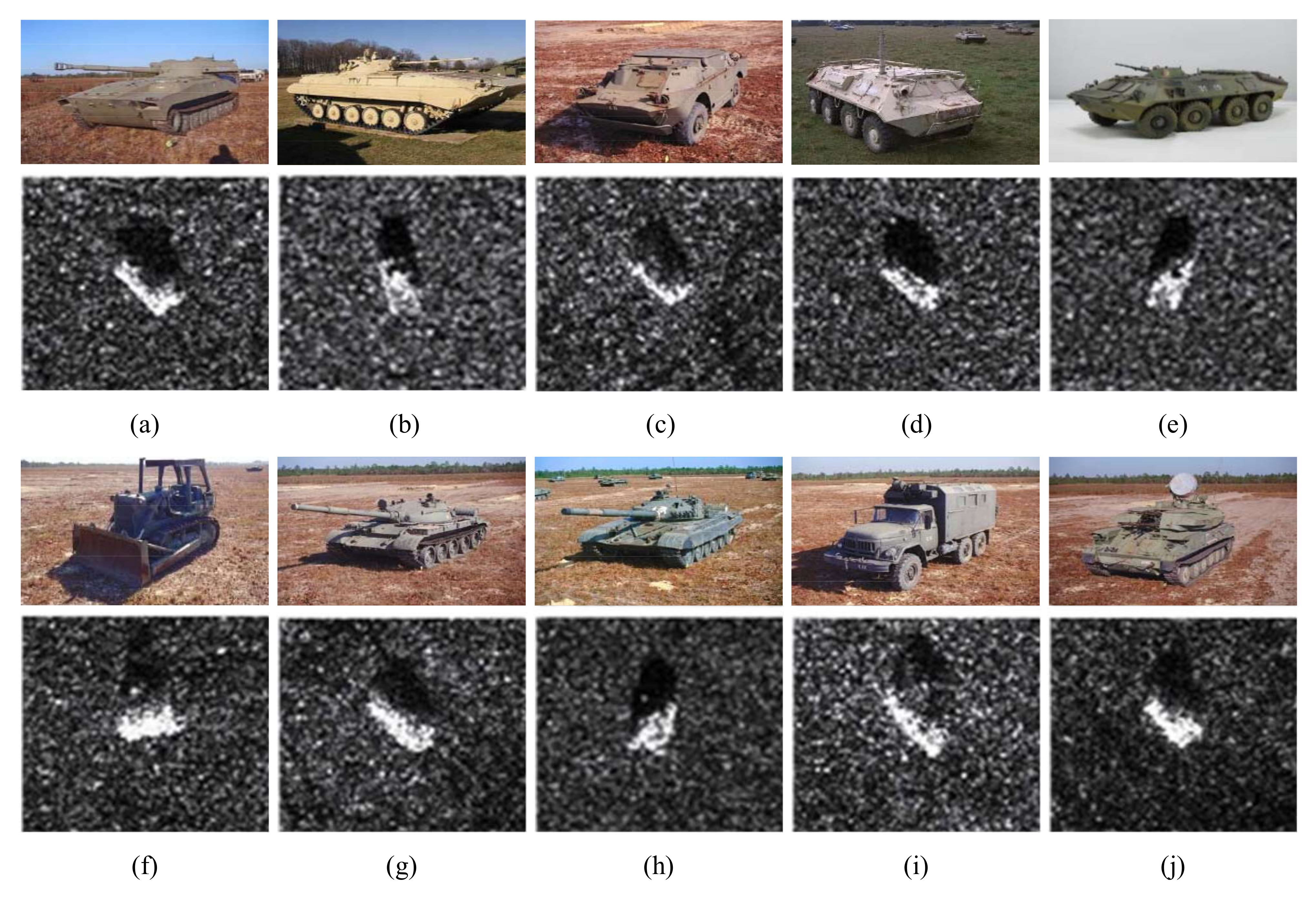
The MSTAR data set [28] is a public data set created by the U.S. Air Force Laboratory, which consists of SAR images of ten classes of military vehicles with ground targets and is divided into two sub-datasets: a training data set and a testing data set. These ten class military vehicles include 2S1, BMP2, BRDM2, BTR60, BTR70, D7, T62, T72, ZIL131, and ZSU234, which are indexed by class labels 1, 2,…,10, respectively. The SAR and the corresponding optical images of each class are shown in Figure 3. The training images are obtained at a depression angle, and the testing images are captured at a depression angle. Each type of target is densely captured in aspect angles, ranging from to . The amount of each category is shown in Table 1.
All the samples are center cropped to pixels. For the semi-supervised training phase, we first divide the training set into two parts: 10, 20, 40, 60, and 80 labeled samples per category are randomly selected, and the rest of the training images are used as unlabeled samples. All the images in the test set are used in the test process.
4.2. Implementation Details
4.2.1. Network Architecture
We use the “Wide-ResNet” model from [29] with depth 28 and width two, which is a popular backbone structure that is widely used in image recognition tasks due to its prominent ability of feature extraction and feature representation. It includes the standard batch normalization [30] and leaky ReLU nonlinearities [31], and the output layer is constructed as a 10-dimensional fully connected layer since the MSTAR data set consists of 10 categories.
4.2.2. Training Setup
Overall, our implementation of the training procedure closely matches that of SCA [23], except for the following differences: We used a batch of 16 images and 200 batches as an epoch. The model was trained for 200 epochs by using the labeled and unlabeled data set, where the Adam [32] optimizer was employed with a learning rate of 0.002 for the model.
To quantitatively evaluate the proposed MBM method, we used the recognition accuracy as the performance metrics. Finally, we conducted five independent experiments on each data set and recorded the average of the best accuracy of these five independent experiments as the final recognition accuracy of the MBM semi-supervised learning method.
The proposed method was tested and evaluated on a computer with Intel Core i7-10070 at 3.80 GHz CPU, GeForce GTX 2080 Ti GPU with 11 GB memory, and 16 GB computer memory. The proposed method was implemented using the open-source Pytorch framework [33].
4.3. Experiments with the Original Training Set under Different Labeled Samples
In the first experiment, we evaluated the performance of the proposed method under different amounts of labeled samples, which were set as 10, 20, 40, 60, and 80 labeled samples per category for the MSTAR data set, and obtained the multi-block mixed semi-supervised recognition accuracy (MBM SSRA). As mentioned above, all these samples were randomly selected, and the samples selected by the five independent experiments were not the same. We also utilized the labeled samples for supervised training by using the same budget of hyperparameter optimization trials and obtained the supervised recognition accuracy (SRA). Table 2 shows the recognition accuracies. As can be seen from Table 2, compared with the model obtained by supervised learning using only labeled samples, the model obtained by using the semi-supervised method can significantly improve the recognition accuracy. When the number of labeled samples was the least, compared with the recognition accuracy of the supervised learning model, the semi-supervised learning model had the best improvement effect in the recognition accuracy, and the relative accuracy was increased to 14.53%. When the number of labeled samples was the largest, the improvement in recognition accuracy was 0.66%. This is also because the accuracy of the supervised learning model reached 99% when there were 80 samples in each category. In other words, the zero-point-six-eight percent improvement was not much better. Specifically, the average relative accuracy improvement was 4.99%. This shows that semi-supervised learning combined with unlabeled data can enable the model to learn more data features and improve recognition accuracy.
From Table 2, we can also know that as the number of labeled data increases, the recognition accuracy of the semi-supervised learning model gradually improves. With only 20 labeled data in each category, the recognition accuracy of the model trained by our semi-supervised learning method completely exceeded the recognition accuracy of all supervised learning models.
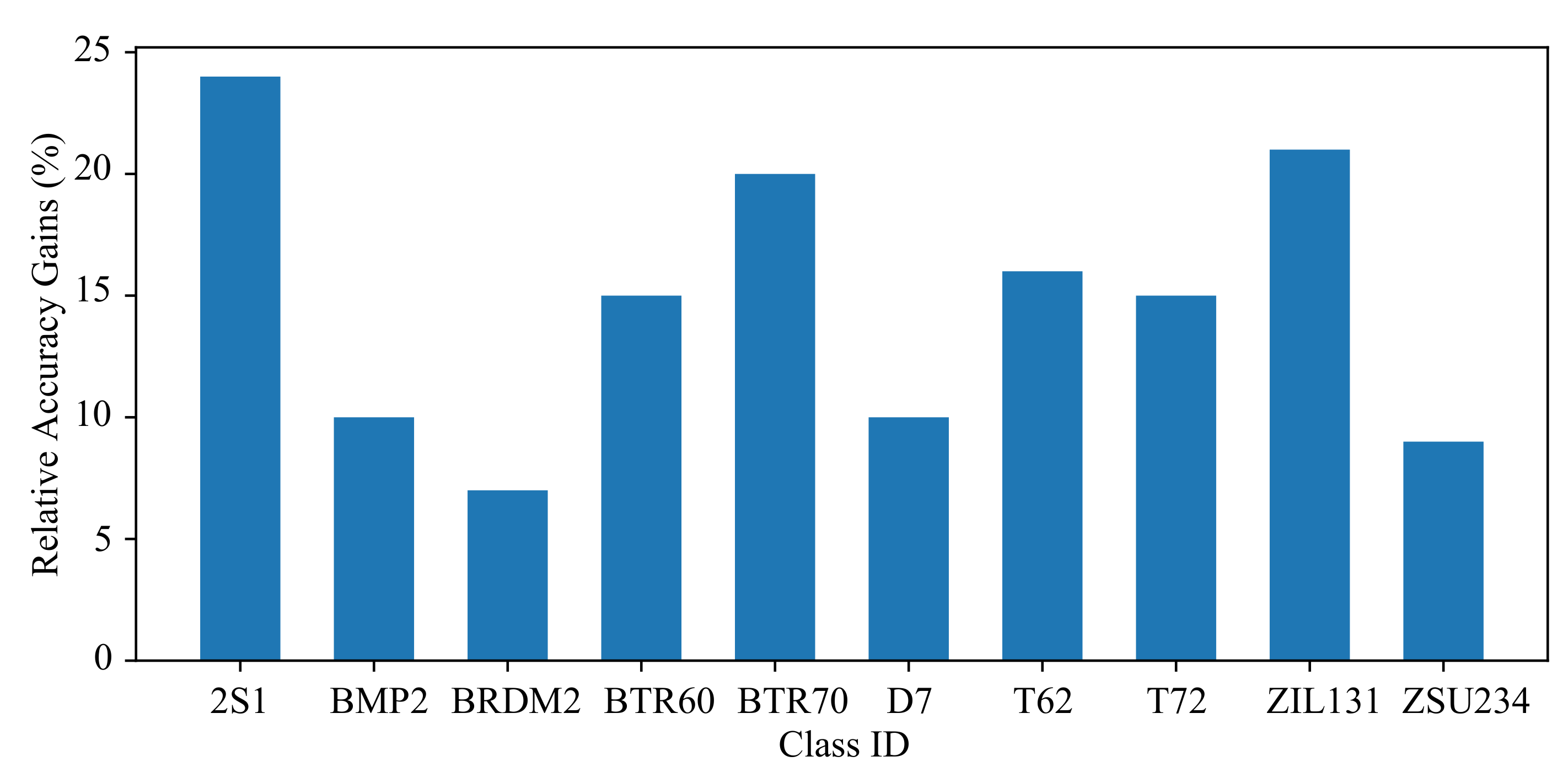
In order to show the improvement of our method on the accuracy of different kinds of object recognition, Figure 4 shows the predicted confusion matrix obtained by the model trained by our method and the model trained by the supervised learning method under 10 labeled samples per category. The recognition accuracy comparison of each category of our method and supervised method when there are 10 labeled samples for each category is shown in Figure 5, which details the improvement of our method relative to the accuracy of the corresponding supervised method in each category.
In the confusion matrices of Figure 4, their entries in the row and column indicate the proportion of samples in which the true label is the type and the predicted label is the type. From the confusion matrix in Figure 4, we can see that our MBM method can achieve 100% prediction recognition accuracy for four categories (i.e., BMRDM2, D7, T72, ZSU234). For the remaining categories, the recognition accuracy rate exceeded 90%, and the recognition accuracy of all categories was generally higher than that of the supervised learning method.
It can be clearly seen from Figure 5 that our MBM method improved the recognition accuracy of all categories by more than 5%. The improvement of BMP2 and ZSU234 was less than 10%, while the improvement of other categories was more than 10%. The improved recognition accuracy of 2S1 and ZIL131 exceeded 20%. In addition, the reason why ZSU234 was not much improved was that the recognition accuracy of the model obtained by the supervised method in the category exceeded 90%, while the improved recognition accuracy was 100%.
4.4. Experiments Comparing Different Mixed Methods
In this section, we conduct ablation experiments. To prove the effectiveness of the MBM method, we used different sample mixing methods, mixup methods, and cutmix methods to prove the recognition performance of our proposed method. To prove the effectiveness of the hybrid method, we also conducted experiments to remove the hybrid method. Table 3 shows the recognition accuracy results of different mixed methods under different numbers of labeled samples.
From Table 3, we can see that our MBM hybrid method provided the best recognition results when the number of labeled samples was small (only 10 labeled samples and 20 labeled samples per class). The cutmix method had the best recognition effect when the number of marked samples was large (the number of samples in each category exceeded 40). It can also be seen from Table 3 that compared to the mixup method, our method can significantly improve the recognition accuracy, especially when the number of labeled samples was very small.
In semi-supervised learning, an important issue is to balance the training of labeled data and unlabeled data, where labeled data and unlabeled data should participate in the entire training process. Mixup generates mixed data to solve the problem of misleading predictions of under-trained classification networks in the early stages of training [23]. Compared with the way that does not use mixed data, mixup can improve classification performance to a certain extent. However, it can be seen from Figure 2 that the image generated by the mixup had certain artifacts, and the image generated by the cutmix was very different from the original image in a large range. To this end, we used the MBM method, which has the advantages of the mixup method, and the new image generated greatly increased the data capacity in the sample space. The most important thing is that the generated image was closer to the original image, so that the model can extract more feature information during the training process. The results in Table 3 fully prove that MBM can improve the recognition performance of the model.
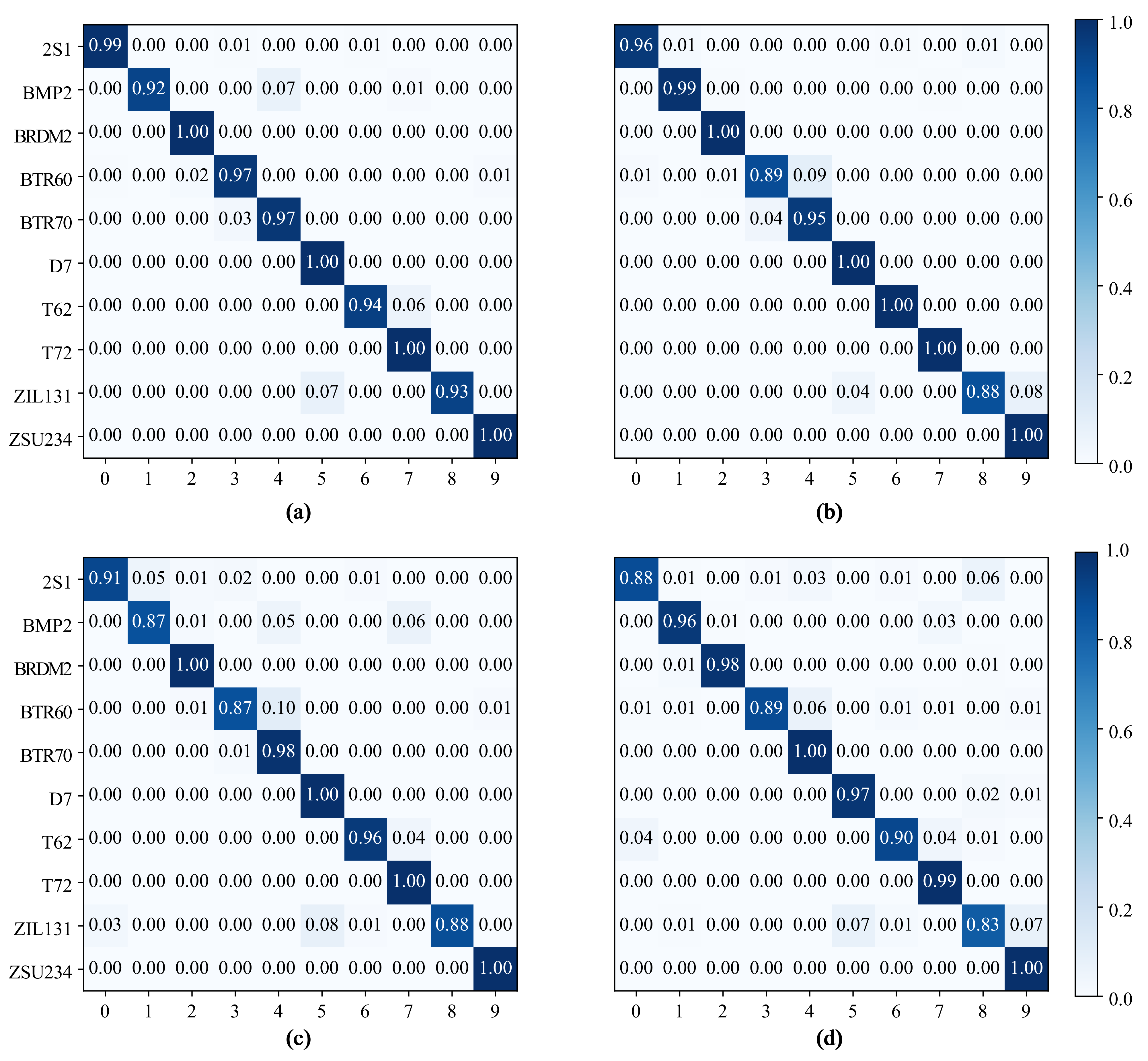
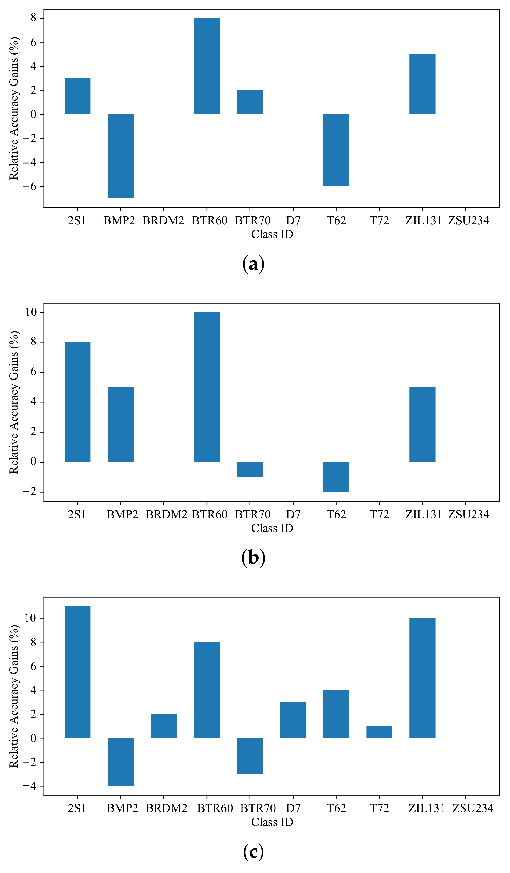
The same as the previous section, to show the improvement of our method on the accuracy of different kinds of object recognition, Figure 6 shows the predicted confusion matrix obtained by the model trained by our method, the model trained by the cutmix semi-supervised learning method, the model trained by the mixup semi-supervised learning method, and the model trained without any hybrid method under 10 labeled samples per category. The recognition accuracy comparison of each category of our method with the cutmix semi-supervised learning method, the mixup semi-supervised learning method, and the non-hybrid semi-supervised method when there were 10 labeled samples for each category is shown in Figure 7, which details the improvement of our method relative to the accuracy of other corresponding mixed semi-supervised learning methods in each category.
From Figure 6 and Figure 7, it can be found that the recognition accuracy of our method and the cutmix method in each category had a small increase compared with the mixup method, and only a certain decrease on BTR70 and T62. Figure 6 shows that the main reason was that the BTR70 target was misidentified as BTR60 and the T62 target was misidentified as T72. In general, our method can bring a certain performance improvement for the semi-supervised learning method based on mixup mixed samples in the recognition task of SAR images.
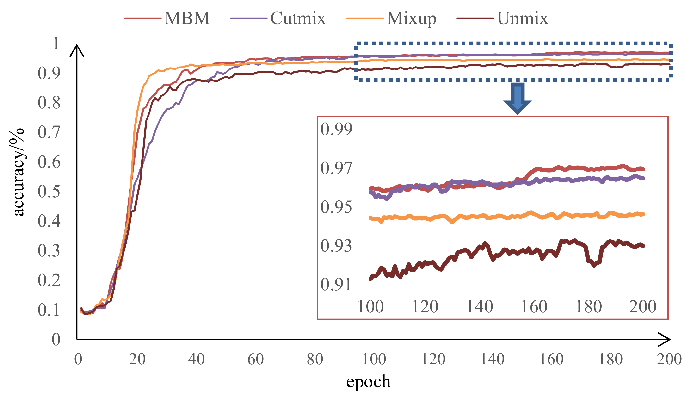
To directly compare the experimental results, we plot the recognition accuracy curves of the MBM, cutmix, mixup, and unmixed methods corresponding to 10 labeled samples per category, as shown in Figure 8. It is observed that the accuracy curve of the mixup method increases the fastest in the initial stage; the MBM method is relatively slow; and the cutmix method increases the slowest. The four kinds of curves are relatively stable after 60 epochs, and MBM obtains the highest recognition accuracy. This indicates that the three hybrid methods can improve the recognition accuracy of the model to a certain extent, and the mixup method can quickly improve the recognition rate in the initial stage. However, as the training process progresses, the training model can better extract the features of the mixed samples provided by the MBM and cutmix methods and achieve higher recognition accuracy. Compared with cutmix, MBM can obtain higher recognition accuracy.
4.5. Experiments Compare with Other Methods
In this part, we compare the performance of our method with several other semi-supervised learning-based SAR ATR methods, including linear neighborhood propagation (LNP) [34], progressive semi-supervised SVM (PSS-SVM) [35], triple-GAN [36], improved-GAN [37], Gao et al.’s method [22], MGAN-CNN [38], and SCA [23] on the MSTAR data set. LNP [34] is a semi-supervised learning approach that establishes a similar matrix and propagates the labels of the labeled samples to the neighborhood unlabeled samples. PSS-SVM [35] expands the original labeled training set by integrating active learning methods, that is selecting reliable unlabeled samples for labeling, thereby increasing labeled samples to optimize the model. Triple-GAN [36] consists of three players, a generator, a discriminator, and a classifier. The generator and the classifier characterize the conditional distributions between images and labels, and the discriminator solely focuses on identifying fake image-label pairs. Improved-GAN [37] utilizes a variety of new architectural features and training procedures, which enables the discriminator to recognize multiple object types. Gao et al. [22] used two discriminators in DCGANto ensure the stable training of GAN by means of joint training and then trained the classifier with samples generated by the generator to improve the recognition performance. SCA [23] trains the recognition model based on consistent regularization and hybrid regularization combined with unlabeled samples using a semi-supervised learning method. In addition to the above methods, we also compared our method with the comparison methods in the above article, such as PCA + SVM [15], AdaBoost [39], SRC [40], K-SVD [41], LCKSVD [42], IGT [43], the Gauss model [44], and DNN-based methods, including DNN1 [45] and DNN2 [46].
Since our method is an improvement based on the SCA method, for a fair comparison, we used the same labeled samples and the same neural network as the recognition model. We conducted five independent experiments by using different labeled samples and selected the average of the five experimental results as the final result. The results of other comparison methods mainly come from articles published for SCA and corresponding methods. Table 4 shows the comparison results.
From Table 4, we see that our MBM method can obtain a higher recognition accuracy with a lower amount of labeled samples. The recognition accuracy is higher than all the other semi-supervised learning methods. Moreover, the recognition accuracy using only 10 labeled samples per category surpassed all other methods except the SCA method. This shows that our method has lower requirements for labeled samples than other semi-supervised learning methods and is more efficient in using unlabeled samples.
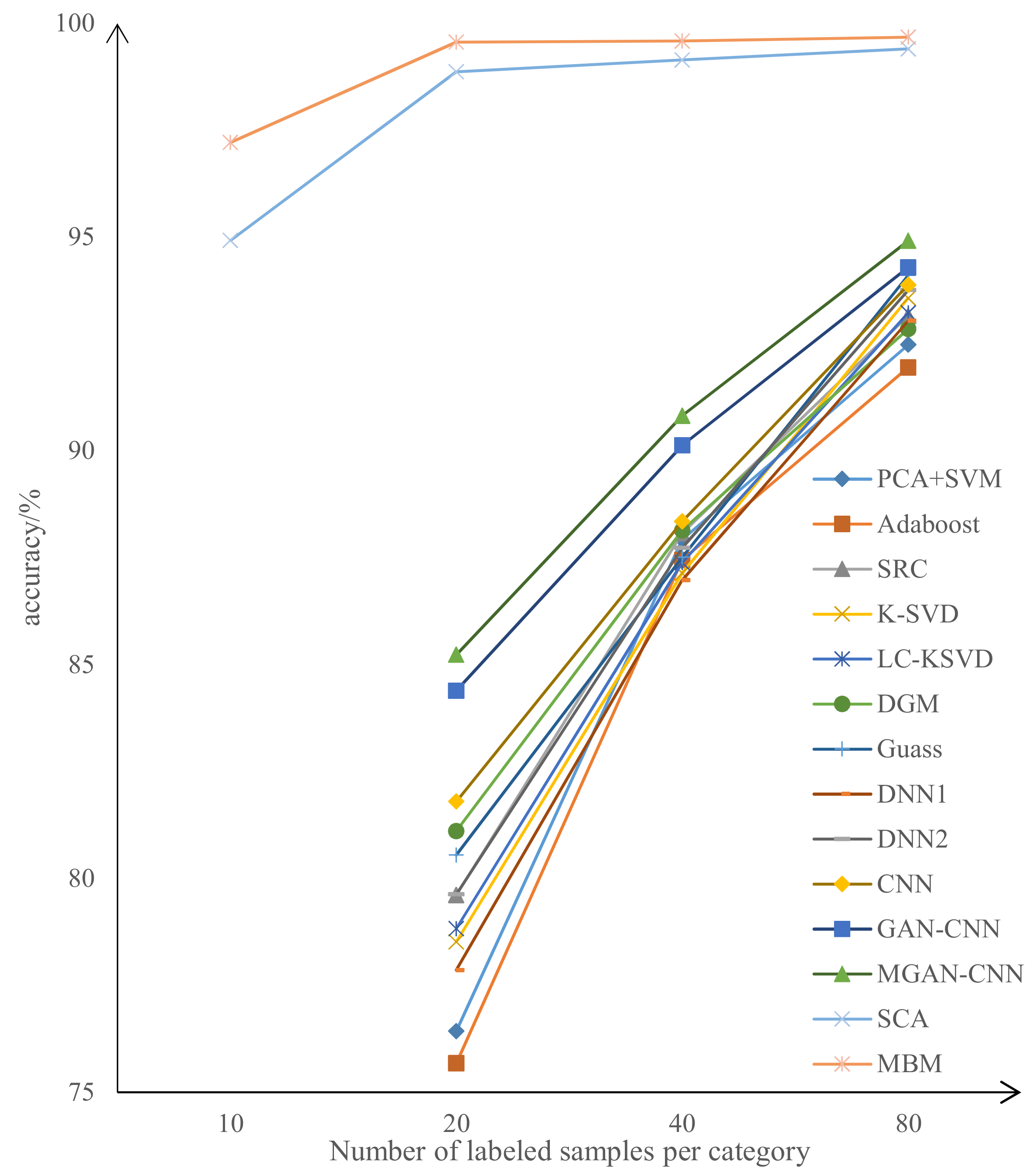
To better compare the performance of our proposed semi-supervised learning method and the methods for comparison with different amounts of labeled training data, we show the recognition accuracies of different methods with different amounts of labeled training data in Figure 9. Compared with Table 4, Figure 9 clearly shows that our method can obtain good recognition results with very few labeled samples. The recognition accuracy rate increases slightly as the number of samples increases. Moreover, compared with other semi-supervised learning methods, only 20 labeled samples per category are enough to achieve the state-of-the-art, which is far less than the other methods based on semi-supervised learning.
5. Discussion
5.1. Choice of Parameter N
In this section, we further discuss the choice of parameter N. The value of N plays a role in adjusting the degree of image fusion. In addition, the higher the N, the more segmented regions of the picture there are and the more mixed blocks of the mixed image there are. Therefore, in this method, the choice of N is very important. We discuss the impact of the N value on the recognition accuracy under different labeled sample sizes.
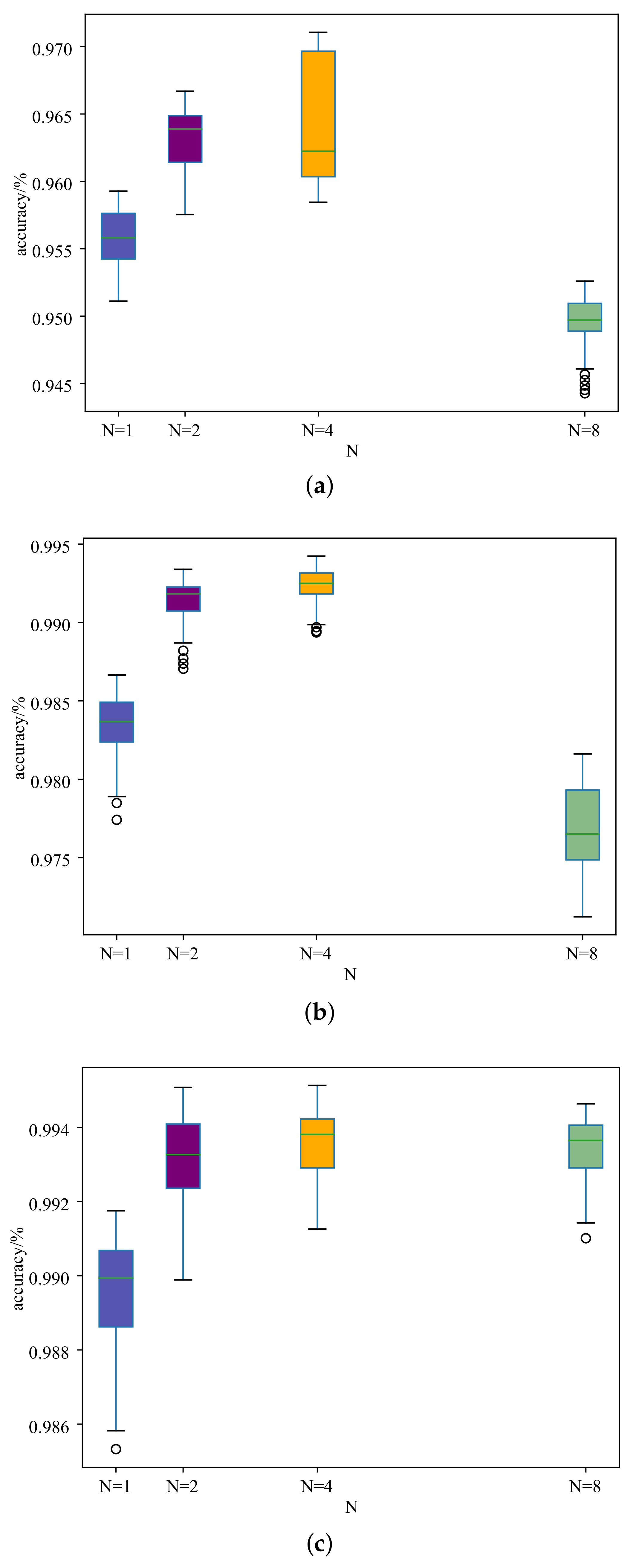
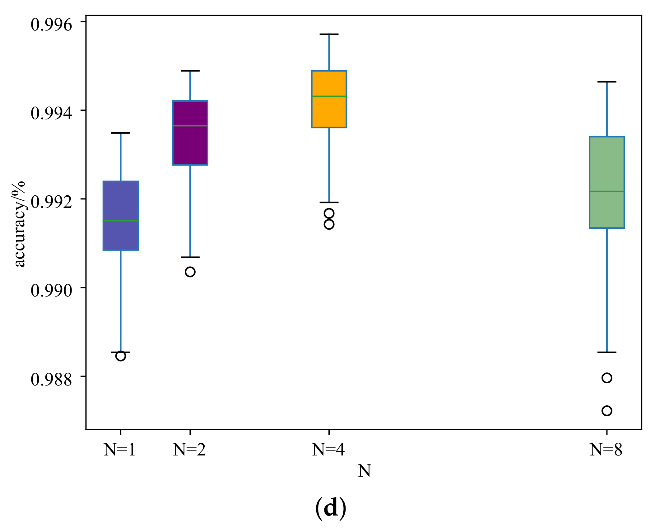
We chose different values, 1, 2, 4, and 8, for N to discuss the influence on the MSTAR data set. We conducted experiments under the conditions that the number of labeled samples in each category were 10, 20, 40, and 60. At the same time, we strictly ensured that other parameters remained unchanged when conducting the experiments. The experimental results are shown in Table 5, and the boxplots of the recognition accuracy with different labeled samples per category are shown in Figure 10.
From Table 5, we can see that the performance is robust to the chosen hyperparameters. The recognition accuracies of different N (1, 2, 4, and 8) for 10 labeled samples per category are 96.17%, 96.84%, 97.21%, and 95.51%, respectively, and for 20 labeled samples per category are 98.85%, 99.51%, 99.56%, and 98.28%, respectively. The trend of the recognition accuracy of 40 labeled samples and 60 labeled samples for each category is also roughly the same. For the same number of labeled samples, i.e., 10, 20, 40, and 60, the maximum improvement is 1.7%, 1.3%, 0.3% and 0.2%, for N values ranging from 1–8. We can see that as the number of labeled samples increases, the maximum improvement effect gradually decreases. This is the same as the trend in Table 2 and is also in line with the general law of semi-supervised learning, that is as the number of samples increases, the recognition effect of the model will also improve. From the results, we can conclude that the method is robust to N in a reasonable range, and the best value for N is four, where the method can obtain the best results for all numbers of labeled samples.
5.2. Time Analysis
Table 6 shows the average running time of MBM, cutmix, mixup, unmixed, and supervised learning without any mixed method in the experiments. In terms of training time, the supervised learning method takes the least training time, and each epoch in the training process takes 7.04 s. The training time of the remaining four semi-supervised learning methods is not much different. Among the semi-supervised learning methods, the unmixed method takes the least time, each epoch taking 17.29 s, and the mixup mixed-method takes the most time, each epoch taking 23.09 s. We believe that mixup mixes the entire picture, making its training time slightly longer than the cutmix and MBM semi-supervised learning methods. Overall, our method can slightly reduce the training time.
The time worth paying attention to is the test time of the model. Mixed samples belong to a data processing method, and this operation is only performed on the training data during the training phase. Whether it is a semi-supervised learning method with mixed data, a semi-supervised learning method without mixing, or a supervised learning method, the Widresnet-28-2 network was used when recognizing SAR images in this article. The processing time for a single image was almost the same for all five methods, and the testing time per image for MBM was 0.512 ms.
6. Conclusions
In this paper, a new sample mixed semi-supervised learning method named MBM is proposed for SAR automatic target recognition. Instead of directly adding two images (i.e., mixup) or covering a whole patch area of another image (i.e., cutmix), our proposed MBM divides the image into multiple blocks and selects a rectangular area in each block to interpolate the corresponding area of another image. In this way, our MBM can add more information without affecting the original image in a large area. Therefore, using the data processed by the MBM method to train a convolution neural network can further improve the recognition accuracy of the model. Experiments on the MSTAR data set confirmed that the MBM method outperforms the current state-of-the-art semi-supervised learning-based methods under different amounts of labeled samples per category. At the same time, when the number of labeled samples is small, compared with supervised learning, the overall recognition accuracy of the model improves more obviously. Using only 10 labeled samples for each category, the model recognition accuracy of our MBM method is improved by 14.54% compared with supervised learning. Under the condition of 20 labeled samples in each category, the recognition accuracy obtained by our MBM method is 99.56%, which is better than the full-sample supervised learning method and all existing semi-supervised learning methods. In future research, we will explore the decisive role of different positions in the same image for identifying labels, so as to change the calculation method of new sample labels, increase the number of samples for generating mixed images, and further improve the recognition performance of semi-supervised learning.
Author Contributions
Y.T., G.Y., and J.S. conceived of and designed the study. Y.T. and P.Q. performed the experiments. Y.T. and L.Z. wrote the paper. G.Y. and J.S. reviewed and edited the manuscript. All authors read and agreed to the published version of the manuscript.
Funding
Our research is funded by the China Postdoctoral Science Foundation No. 2019M661319, the Fundamental Research Funds for the Central Universities (3072020CFQ-0602, 3072020CF0604, 3072020CFP0601), and 2019 Industrial Internet Innovation and Development Engineering (KY1060020002, KY10600200008).
Institutional Review Board Statement
The study not involving humans or animals.
Informed Consent Statement
The study not involving humans.
Data Availability Statement
The experiment in this paper uses a public data set, so no data is reported in this work.
Conflicts of Interest
The authors declare that they have no conflicts of interest to report regarding the present study.
References
- Bai, X.; Xue, R.; Wang, L.; Zhou, F. Sequence SAR Image Classification Based on Bidirectional Convolution-Recurrent Network. IEEE Trans. Geosci. Remote. Sens. 2019, 57, 9223–9235. [Google Scholar] [CrossRef]
- Xu, H.; Yang, Z.; Tian, M.; Sun, Y.; Liao, G. An extended moving target detection approach for high-resolution multichannel SAR-GMTI systems based on enhanced shadow-aided decision. IEEE Trans. Geosci. Remote. Sens. 2017, 56, 715–729. [Google Scholar] [CrossRef]
- Clemente, C.; Pallotta, L.; Gaglione, D.; De Maio, A.; Soraghan, J.J. Automatic Target Recognition of Military Vehicles with Krawtchouk Moments. IEEE Trans. Aerosp. Electron. Syst. 2017, 53, 493–500. [Google Scholar] [CrossRef] [Green Version]
- Tait, P. Introduction to Radar Target Recognition; IET: London, UK, 2005; Volume 18. [Google Scholar]
- Zhai, Y.; Deng, W.; Lan, T.; Sun, B.; Ying, Z.; Gan, J.; Mai, C.; Li, J.; Labati, R.D.; Piuri, V.; et al. MFFA-SARNET: Deep Transferred Multi-Level Feature Fusion Attention Network with Dual Optimized Loss for Small-Sample SAR ATR. Remote Sens. 2020, 12, 1385. [Google Scholar] [CrossRef]
- Kechagias-Stamatis, O. Automatic Target Recognition on Synthetic Aperture Radar Imagery: A Survey. arXiv 2020, arXiv:2007.02106. [Google Scholar]
- Clemente, C.; Pallotta, L.; Proudler, I.; De Maio, A.; Soraghan, J.J.; Farina, A. Pseudo-Zernike-based multi-pass automatic target recognition from multi-channel synthetic aperture radar. IET Radar Sonar Navig. 2015, 9, 457–466. [Google Scholar] [CrossRef] [Green Version]
- Sun, Y.; Du, L.; Wang, Y.; Wang, Y.; Hu, J. SAR automatic target recognition based on dictionary learning and joint dynamic sparse representation. IEEE Geosci. Remote. Sens. Lett. 2016, 13, 1777–1781. [Google Scholar] [CrossRef]
- Novak, L.M.; Benitz, G.R.; Owirka, G.J.; Bessette, L.A. ATR performance using enhanced resolution SAR. In Algorithms for Synthetic Aperture Radar Imagery III; International Society for Optics and Photonics: Bellingham, WA, USA, 1996; Volume 2757, pp. 332–337. [Google Scholar] [CrossRef]
- El-Darymli, K.; Gill, E.W.; McGuire, P.; Power, D.; Moloney, C. Automatic target recognition in synthetic aperture radar imagery: A state-of-the-art review. IEEE Access 2016, 4, 6014–6058. [Google Scholar] [CrossRef] [Green Version]
- Zhong, C.; Mu, X.; He, X.; Wang, J.; Zhu, M. SAR Target Image Classification Based on Transfer Learning and Model Compression. IEEE Geosci. Remote. Sens. Lett. 2019, 16, 412–416. [Google Scholar] [CrossRef]
- Huang, Z.; Pan, Z.; Lei, B. Transfer learning with deep convolutional neural network for SAR target classification with limited labeled data. Remote Sens. 2017, 9, 907. [Google Scholar] [CrossRef] [Green Version]
- Kim, S.; Song, W.J.; Kim, S.H. Double weight-based SAR and infrared sensor fusion for automatic ground target recognition with deep learning. Remote Sens. 2018, 10, 72. [Google Scholar] [CrossRef] [Green Version]
- Shi, X.; Zhou, F.; Yang, S.; Zhang, Z.; Su, T. Automatic target recognition for synthetic aperture radar images based on super-resolution generative adversarial network and deep convolutional neural network. Remote Sens. 2019, 11, 135. [Google Scholar] [CrossRef] [Green Version]
- Zhao, Q.; Principe, J.C. Support vector machines for SAR automatic target recognition. IEEE Trans. Aerosp. Electron. Syst. 2001, 37, 643–654. [Google Scholar] [CrossRef] [Green Version]
- Huang, Z.; Pan, Z.; Lei, B. What, Where, and How to Transfer in SAR Target Recognition Based on Deep CNNs. IEEE Trans. Geosci. Remote. Sens. 2020, 58, 2324–2336. [Google Scholar] [CrossRef] [Green Version]
- Tang, K.; Sun, X.; Sun, H.; Wang, H. A geometrical-based simulator for target recognition in high-resolution SAR images. IEEE Geosci. Remote. Sens. Lett. 2012, 9, 958–962. [Google Scholar] [CrossRef]
- Huang, Z.; Dumitru, C.O.; Pan, Z.; Lei, B.; Datcu, M. Classification of large-scale high-resolution sar images with deep transfer learning. IEEE Geosci. Remote. Sens. Lett. 2020. [Google Scholar] [CrossRef] [Green Version]
- Zhang, M.; An, J.; Yang, L.D.; Wu, L.; Lu, X.Q. Convolutional Neural Network With Attention Mechanism for SAR Automatic Target Recognition. IEEE Geosci. Remote. Sens. Lett. 2020. [Google Scholar] [CrossRef]
- Li, Y.; Li, X.; Sun, Q.; Dong, Q. SAR Image Classification Using CNN Embeddings and Metric Learning. IEEE Geosci. Remote. Sens. Lett. 2020, 1–5. [Google Scholar] [CrossRef]
- Zhang, F.; Wang, Y.; Ni, J.; Zhou, Y.; Hu, W. SAR Target Small Sample Recognition Based on CNN Cascaded Features and AdaBoost Rotation Forest. IEEE Geosci. Remote. Sens. Lett. 2020, 17, 1008–1012. [Google Scholar] [CrossRef]
- Gao, F.; Yang, Y.; Wang, J.; Sun, J.; Yang, E.; Zhou, H. A deep convolutional generative adversarial networks (DCGANs)-based semi-supervised method for object recognition in synthetic aperture radar (SAR) images. Remote Sens. 2018, 10, 846. [Google Scholar] [CrossRef] [Green Version]
- Wang, C.; Shi, J.; Zhou, Y.; Yang, X.; Zhou, Z.; Wei, S.; Zhang, X. Semisupervised Learning-Based SAR ATR via Self-Consistent Augmentation. IEEE Trans. Geosci. Remote. Sens. 2020, 1–12. [Google Scholar] [CrossRef]
- Zhang, H.; Cisse, M.; Dauphin, Y.N.; Lopez-Paz, D. mixup: Beyond Empirical Risk Minimization. In Proceedings of the International Conference on Learning Representations, Vancouver, BC, Canada, 30 April–3 May 2018. [Google Scholar]
- Yun, S.; Han, D.; Oh, S.J.; Chun, S.; Choe, J.; Yoo, Y. Cutmix: Regularization strategy to train strong classifiers with localizable features. In Proceedings of the IEEE International Conference on Computer Vision, Seoul, Korea, 27 October–2 November 2019; pp. 6023–6032. [Google Scholar]
- DeVries, T.; Taylor, G.W. Improved regularization of convolutional neural networks with cutout. arXiv 2017, arXiv:1708.04552. [Google Scholar]
- Ross, T.D.; Worrell, S.W.; Velten, V.J.; Mossing, J.C.; Bryant, M.L. Standard SAR ATR evaluation experiments using the MSTAR public release data set. In Algorithms for Synthetic Aperture Radar Imagery V; International Society for Optics and Photonics: Bellingham, WA, USA, 1998; Volume 3370, pp. 566–573. [Google Scholar]
- Keydel, E.R.; Lee, S.W.; Moore, J.T. MSTAR extended operating conditions: A tutorial. In Algorithms for Synthetic Aperture Radar Imagery III; International Society for Optics and Photonics: Bellingham, WA, USA, 1996; Volume 2757, pp. 228–242. [Google Scholar]
- Zagoruyko, S.; Komodakis, N. Wide residual networks. In Proceedings of the British Machine Vision Conference (BMVC), York, UK, 19–22 September 2016. [Google Scholar]
- Ioffe, S.; Szegedy, C. Batch Normalization: Accelerating Deep Network Training by Reducing Internal Covariate Shift. In Proceedings of the International Conference on Machine Learning, Lille, France, 6–11 July 2015; pp. 448–456. [Google Scholar]
- Maas, A.L.; Hannun, A.Y.; Ng, A.Y. Rectifier nonlinearities improve neural network acoustic models. In Proceedings of the 30th International Conference on Machine Learning, Atlanta, GA, USA, 17–19 June 2013; Volume 30, p. 3. [Google Scholar]
- Kingma, D.P.; Ba, J.L. Adam: A method for stochastic optimization. In Proceedings of the Second International Conference on Learning Representations, Banff, AB, Canada, 14–16 April 2014. [Google Scholar]
- Paszke, A.; Gross, S.; Massa, F.; Lerer, A.; Bradbury, J.; Chanan, G.; Killeen, T.; Lin, Z.; Gimelshein, N.; Antiga, L.; et al. Pytorch: An imperative style, high-performance deep learning library. In Proceedings of the 33rd International Conference on Neural Information Processing Systems, Vancouver, BC, Canda, 8–14 December 2019; pp. 8026–8037. [Google Scholar]
- Wang, F.; Zhang, C. Label propagation through linear neighborhoods. IEEE Trans. Knowl. Data Eng. 2007, 20, 55–67. [Google Scholar] [CrossRef]
- Persello, C.; Bruzzone, L. Active and semisupervised learning for the classification of remote sensing images. IEEE Trans. Geosci. Remote. Sens. 2014, 52, 6937–6956. [Google Scholar] [CrossRef]
- Li, C.; Xu, K.; Zhu, J.; Zhang, B. Triple generative adversarial nets. In Proceedings of the 31st International Conference on Neural Information Processing Systems, California, CA, USA, 4–9 December 2017; pp. 4091–4101. [Google Scholar]
- Salimans, T.; Goodfellow, I.; Zaremba, W.; Cheung, V.; Radford, A.; Chen, X. Improved techniques for training gans. In Proceedings of the 30th International Conference on Neural Information Processing Systems, Barcelona, Spain, 5–10 December 2016; pp. 2234–2242. [Google Scholar]
- Zheng, C.; Jiang, X.; Liu, X. Semi-supervised SAR ATR via multi-discriminator generative adversarial network. IEEE Sens. J. 2019, 19, 7525–7533. [Google Scholar] [CrossRef]
- Sun, Y.; Liu, Z.; Todorovic, S.; Li, J. Adaptive boosting for SAR automatic target recognition. IEEE Trans. Aerosp. Electron. Syst. 2007, 43, 112–125. [Google Scholar] [CrossRef]
- Zhang, H.; Nasrabadi, N.M.; Zhang, Y.; Huang, T.S. Multi-view automatic target recognition using joint sparse representation. IEEE Trans. Aerosp. Electron. Syst. 2012, 48, 2481–2497. [Google Scholar] [CrossRef]
- Aharon, M.; Elad, M.; Bruckstein, A. K-SVD: An algorithm for designing overcomplete dictionaries for sparse representation. IEEE Trans. Signal Process. 2006, 54, 4311–4322. [Google Scholar] [CrossRef]
- Jiang, Z.; Lin, Z.; Davis, L.S. Label consistent K-SVD: Learning a discriminative dictionary for recognition. IEEE Trans. Pattern Anal. Mach. Intell. 2013, 35, 2651–2664. [Google Scholar] [CrossRef]
- Srinivas, U.; Monga, V.; Raj, R.G. SAR automatic target recognition using discriminative graphical models. IEEE Trans. Aerosp. Electron. Syst. 2014, 50, 591–606. [Google Scholar] [CrossRef]
- O’Sullivan, J.A.; DeVore, M.D.; Kedia, V.; Miller, M.I. SAR ATR performance using a conditionally Gaussian model. IEEE Trans. Aerosp. Electron. Syst. 2001, 37, 91–108. [Google Scholar] [CrossRef] [Green Version]
- Morgan, D.A. Deep convolutional neural networks for ATR from SAR imagery. In Algorithms for Synthetic Aperture Radar Imagery XXII; International Society for Optics and Photonics: Bellingham, WA, USA, 2015; Volume 9475, p. 94750F. [Google Scholar]
- Ding, J.; Chen, B.; Liu, H.; Huang, M. Convolutional neural network with data augmentation for SAR target recognition. IEEE Geosci. Remote. Sens. Lett. 2016, 13, 364–368. [Google Scholar] [CrossRef]
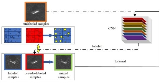
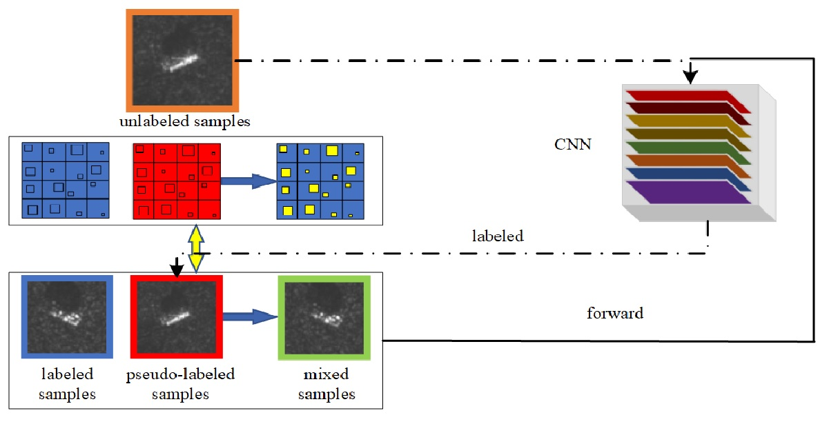
Figure 1.
The framework for the self-consistent augmentation (SCA) method, where the training procedure includes three phases: sample labeling, data processing, and model training. In particular, sample labeling is part of data processing. First, in the early stages of data processing, SCA performs data augmentation on labeled and unlabeled samples. At this time, the model pseudo-labels unlabeled samples. Then, there is the later stage of data processing, where the labeled samples and pseudo-labeled samples are combined, and the combined data set and randomly shuffled combined data set are mixed to obtain a new sample set. Finally, the new sample set is used to train the model.

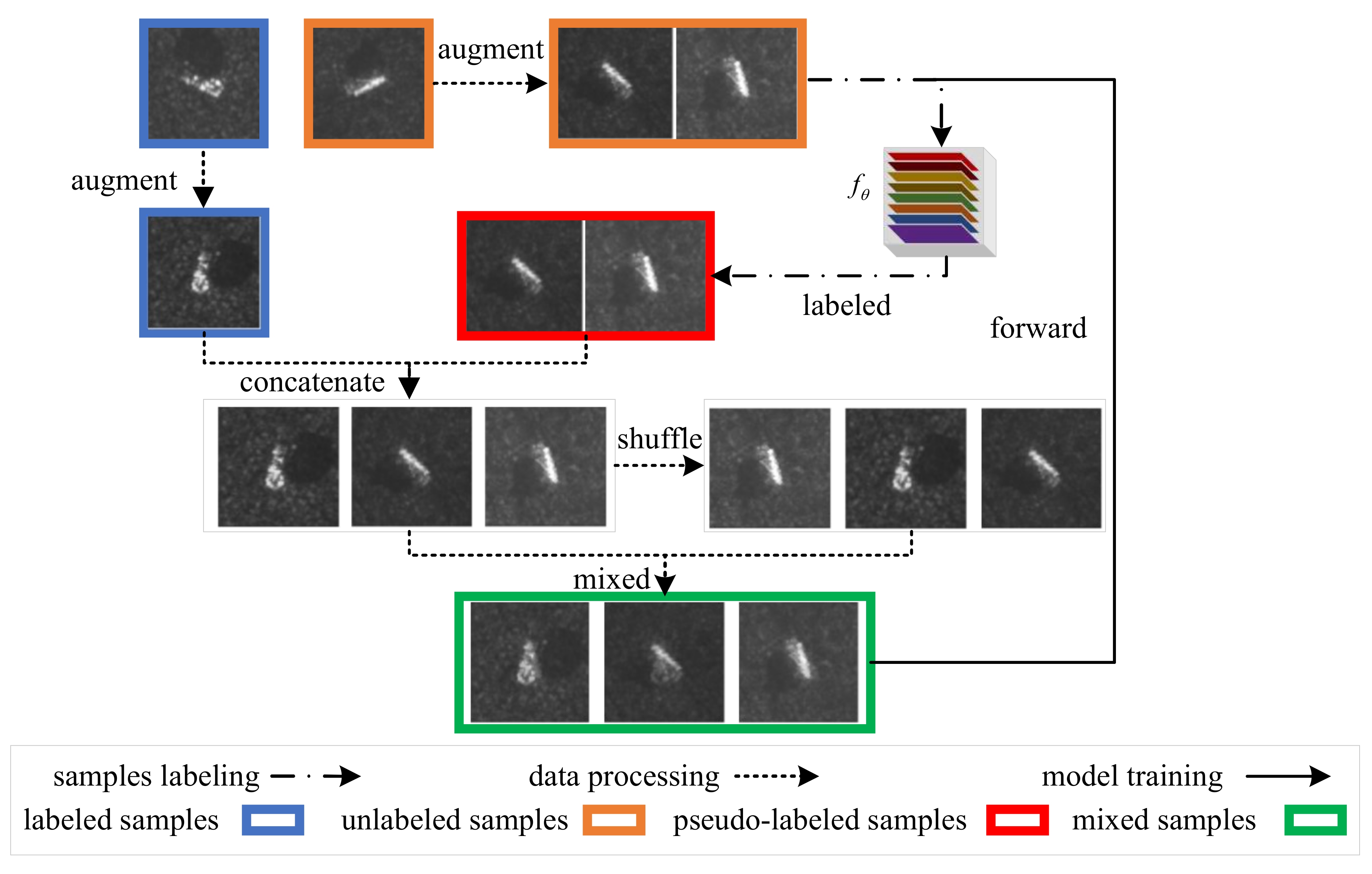
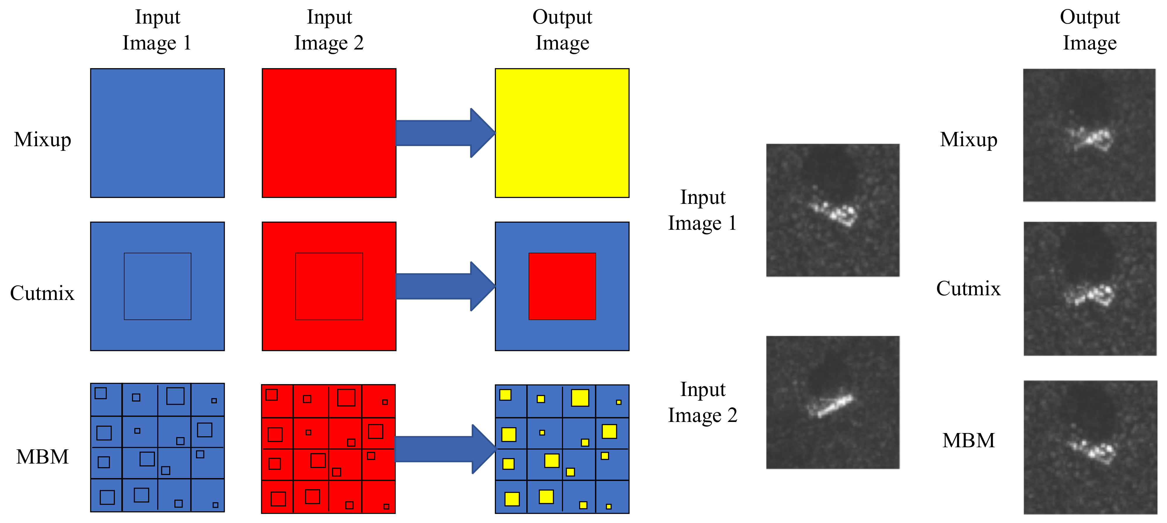
Figure 2.
Overview of mixup, cutmix, and our multi-block mixed (MBM) blending methods. The left part of the figure is an example of the operation of the three hybrid methods. Among them, the mixup method performs interpolation operations on the input image; the cutmix method introduces an additional matrix (omitted in the figure) and uses element-wise multiplication to replace part of the content in the input image; the MBM method divides the picture into N parts and selects a small part of each part and the corresponding part of another input image for interpolation and mixing. The input SAR images of the three methods and the new samples generated are shown on the right side of the figure, and the generation method does not strictly correspond to the frame selection position in the left figure.

Figure 3.
Optical images and corresponding SAR images of ten classes of objects in the moving and stationary target acquisition and recognition (MSTAR) database, (a) 2S1; (b) BMP2; (c) BRDM2; (d) BTR60; (e) BTR70; (f) D7; (g) T62; (h) T72; (i) ZIL131; (j) ZSU234.
Figure 3.
Optical images and corresponding SAR images of ten classes of objects in the moving and stationary target acquisition and recognition (MSTAR) database, (a) 2S1; (b) BMP2; (c) BRDM2; (d) BTR60; (e) BTR70; (f) D7; (g) T62; (h) T72; (i) ZIL131; (j) ZSU234.

Figure 4.
Confusion matrices of the proposed method and the corresponding supervised method under 10 labeled samples per category: (a) MBM; (b) supervised method.
Figure 4.
Confusion matrices of the proposed method and the corresponding supervised method under 10 labeled samples per category: (a) MBM; (b) supervised method.

Figure 5.
Precision comparison for each class of the MBM and the corresponding supervised method, where the Y-axis denotes per class classification accuracy improvement of the MBM relative to the corresponding supervised method, and the X-axis denotes the class index of each category.
Figure 5.
Precision comparison for each class of the MBM and the corresponding supervised method, where the Y-axis denotes per class classification accuracy improvement of the MBM relative to the corresponding supervised method, and the X-axis denotes the class index of each category.

Figure 6.
Confusion matrices of the proposed method and other mixed semi-supervised learning methods under 10 labeled samples per category (a) MBM; (b) cutmix; (c) mixup; (d) unmixed. The average performance per method is 97.21%, 96.75%, 94.92%, and 93.75%.
Figure 6.
Confusion matrices of the proposed method and other mixed semi-supervised learning methods under 10 labeled samples per category (a) MBM; (b) cutmix; (c) mixup; (d) unmixed. The average performance per method is 97.21%, 96.75%, 94.92%, and 93.75%.

Figure 7.
Precision comparisons for each class of the MBM and other mixed semi-supervised methods, where the Y-axis denotes the per class classification accuracy improvement of the MBM relative to another mixed semi-supervised method, and the X-axis denotes the class index of each category. (a) MBM and cutmix; (b) MBM and mixup; (c) MBM and unmixed.

Figure 8.
Recognition accuracy curves of the MBM, cutmix, mixup, and unmixed methods under 10 labeled samples per category.
Figure 8.
Recognition accuracy curves of the MBM, cutmix, mixup, and unmixed methods under 10 labeled samples per category.

Figure 9.
Recognition accuracies of the proposed semi-supervised learning method and the methods for comparison on the MSTAR data set.
Figure 9.
Recognition accuracies of the proposed semi-supervised learning method and the methods for comparison on the MSTAR data set.

Figure 10.
Boxplots of the recognition accuracy of different N values under different labeled samples in each category on the MSTAR data set. (a) 10; (b) 20; (c) 40; (d) 80.
Figure 10.
Boxplots of the recognition accuracy of different N values under different labeled samples in each category on the MSTAR data set. (a) 10; (b) 20; (c) 40; (d) 80.


Table 1.
Detailed information of the MSTAR data set used in our experiments.
| Tops | Class | Training Set | Testing Set | All Data | ||
|---|---|---|---|---|---|---|
| Depression | No. of Images | Depression | No. of Images | No. of Images | ||
| Artillery | 2S1 | 299 | 274 | 573 | ||
| ZSU234 | 299 | 274 | 573 | |||
| Tank | T62 | 299 | 273 | 572 | ||
| T72 | 232 | 196 | 428 | |||
| Truck | BRDM2 | 298 | 274 | 572 | ||
| BTR60 | 256 | 195 | 451 | |||
| BTR70 | 233 | 196 | 429 | |||
| BMP2 | 233 | 195 | 428 | |||
| D7 | 299 | 274 | 573 | |||
| ZIL131 | 299 | 274 | 573 | |||
| Total | —— | —— | 2747 | —— | 2425 | 5172 |
Table 2.
Recognition accuracies of the proposed semi-supervised learning method and the corresponding supervised method under different amounts of labeled samples per category on the MSTAR data set. SSRA, semi-supervised recognition accuracy.
Table 2.
Recognition accuracies of the proposed semi-supervised learning method and the corresponding supervised method under different amounts of labeled samples per category on the MSTAR data set. SSRA, semi-supervised recognition accuracy.
| Number of Labeled Samples Per Category | ||||||
|---|---|---|---|---|---|---|
| 10 | 20 | 40 | 60 | 80 | Full | |
| MBM SSRA | 97.21 ± 2.441 | 99.56 ± 0.155 | 99.58 ± 0.074 | 99.65 ± 0.062 | 99.67 ± 0.034 | - |
| SRA | 82.67 ± 3.236 | 93.23 ± 1.339 | 97.27 ± 0.467 | 98.516 ± 0.262 | 99.01 ± 0.121 | 99.53 ± 0.074 |
Table 3.
Recognition accuracies of the proposed semi-supervised learning method, cutmix semi-supervised learning method, mixup semi-supervised learning method, and unmixed semi-supervised learning method under different amounts of labeled samples per category on the MSTAR data set. The bold numbers represent the optimal value in each column.
| Number of Labeled Samples Per Category | |||||
|---|---|---|---|---|---|
| 10 | 20 | 40 | 60 | 80 | |
| MBM SSRA | 97.21 ± 2.441 | 99.56 ± 0.155 | 99.58 ± 0.074 | 99.65 ± 0.062 | 99.67 ± 0.034 |
| cutmix SSRA | 96.74 ± 2.011 | 99.28 ± 0.638 | 99.66 ± 0.074 | 99.71 ± 0.133 | 99.71 ± 0.065 |
| mixup SSRA | 94.92 ± 4.359 | 98.86 ± 0.447 | 99.14 ± 0.259 | 99.11 ± 0.255 | 99.40 ± 0.150 |
| unmix SSRA | 93.75 ± 3.602 | 98.82 ± 0.313 | 98.99 ± 0.340 | 99.20 ± 0.147 | 99.36 ± 0.135 |
Table 4.
Recognition accuracies of the proposed semi-supervised learning method and other semi-supervised methods under different amounts of labeled samples per category on the MSTAR data set. The bold numbers represent the optimal value in each column. Hyphens indicate that accuracy is not present in the published article.
| Number of Labeled Samples Per Category | |||||
|---|---|---|---|---|---|
| 10 | 20 | 40 | 55 | 80 | |
| LNP | - | - | - | 92.04 | - |
| PSS-SVM | - | - | - | 95.01 | - |
| Triple-GAN | - | - | - | 95.70 | - |
| Improved-GAN | - | - | - | 87.52 | - |
| Gao et al. | - | - | - | 95.72 | - |
| PCA+SVM | - | 76.43 | 87.92 | - | 92.48 |
| AdaBoost | - | 75.68 | 87.45 | - | 91.95 |
| SRC | - | 79.61 | 88.07 | - | 93.16 |
| K-SVD | - | 78.52 | 87.14 | - | 93.57 |
| 10 | 20 | 40 | 55 | 80 | |
| LC-KSVD | - | 78.83 | 87.39 | - | 93.23 |
| DGM | - | 81.11 | 88.14 | - | 92.85 |
| Gauss | - | 80.55 | 87.51 | - | 94.10 |
| DNN1 | - | 77.86 | 86.98 | - | 93.04 |
| DNN2 | - | 79.63 | 87.73 | - | 93.76 |
| CNN | - | 81.80 | 88.35 | - | 93.88 |
| GAN-CNN | - | 84.39 | 90.13 | - | 94.29 |
| MGAN-CNN | - | 85.23 | 90.82 | - | 94.91 |
| SCA | 94.92 ± 4.359 | 98.86 ± 1.242 | 99.14 ± 0.259 | 99.12 ± 0.345 | 99.40 ± 0.150 |
| MBM (our proposal) | 97.21 ± 2.441 | 99.56 ± 0.155 | 99.58 ± 0.074 | 99.63 ± 0.067 | 99.67 ± 0.034 |
Table 5.
Recognition accuracies of the proposed semi-supervised learning method for different N values under different amounts of labeled samples per category on the MSTAR data set. The bold numbers represent the optimal value in each column.
Table 5.
Recognition accuracies of the proposed semi-supervised learning method for different N values under different amounts of labeled samples per category on the MSTAR data set. The bold numbers represent the optimal value in each column.
| Value of N | Number of Labeled Samples Per Category | |||
|---|---|---|---|---|
| 10 | 20 | 40 | 60 | |
| 1 | 96.17 ± 2.652 | 98.85 ± 0.711 | 99.29 ± 0.525 | 99.48 ± 0.046 |
| 2 | 96.84 ± 3.091 | 99.51 ± 0.107 | 99.55 ± 0.073 | 99.60 ± 0.094 |
| 4 | 97.21 ± 2.441 | 99.56 ± 0.155 | 99.58 ± 0.074 | 99.65 ± 0.067 |
| 8 | 95.51 ± 2.002 | 98.28 ± 1.828 | 99.56 ± 0.094 | 99.57 ± 0.102 |
Table 6.
Time analysis of the proposed method, cutmix, mixup, unmixed, and the supervised learning method.
Table 6.
Time analysis of the proposed method, cutmix, mixup, unmixed, and the supervised learning method.
| Training Time Per Epoch | Testing Time Per Image | |
|---|---|---|
| MBM | 17.28 s | 0.512 ms |
| cutmix | 17.57 s | 0.531 ms |
| mixup | 23.09 s | 0.511 ms |
| unmixed | 17.29 s | 0.522 ms |
| supervised method | 7.04 s | 0.518 ms |
Publisher’s Note: MDPI stays neutral with regard to jurisdictional claims in published maps and institutional affiliations. |
© 2021 by the authors. Licensee MDPI, Basel, Switzerland. This article is an open access article distributed under the terms and conditions of the Creative Commons Attribution (CC BY) license (http://creativecommons.org/licenses/by/4.0/).
Share and Cite
MDPI and ACS Style
Tian, Y.; Sun, J.; Qi, P.; Yin, G.; Zhang, L. Multi-Block Mixed Sample Semi-Supervised Learning for SAR Target Recognition. Remote Sens. 2021, 13, 361. https://0-doi-org.brum.beds.ac.uk/10.3390/rs13030361
AMA Style
Tian Y, Sun J, Qi P, Yin G, Zhang L. Multi-Block Mixed Sample Semi-Supervised Learning for SAR Target Recognition. Remote Sensing. 2021; 13(3):361. https://0-doi-org.brum.beds.ac.uk/10.3390/rs13030361
Chicago/Turabian StyleTian, Ye, Jianguo Sun, Pengyuan Qi, Guisheng Yin, and Liguo Zhang. 2021. "Multi-Block Mixed Sample Semi-Supervised Learning for SAR Target Recognition" Remote Sensing 13, no. 3: 361. https://0-doi-org.brum.beds.ac.uk/10.3390/rs13030361
Note that from the first issue of 2016, this journal uses article numbers instead of page numbers. See further details here.