
Sub-Auroral, Mid-Latitude, and Low-Latitude Troughs during Severe Geomagnetic Storms

Pushkov Institute of Terrestrial Magnetism, Ionosphere, and Radiowave Propagation, (IZMIRAN), 4, Kaluzhskoe Hwy, Troitsk, 108840 Moscow, Russia
Remote Sens. 2021, 13(3), 534; https://0-doi-org.brum.beds.ac.uk/10.3390/rs13030534
Submission received: 15 December 2020
/
Revised: 17 January 2021
/
Accepted: 29 January 2021
/
Published: 2 February 2021
(This article belongs to the Special Issue Space Weather: Observations and Modeling of the Near Earth Environment)
Abstract
:The dynamics of ionospheric troughs during intense geomagnetic storms is considered in this paper. The study is based on electron density measurements at CHAMP satellite altitudes of 405–465 km in the period from 2000 to 2002. A detailed analysis of four storms with Kp from 5+ to 9− is presented. Three troughs were identified: sub-auroral, mid-latitude, and low-latitude. The sub-auroral trough is usually defined as the main ionospheric trough (MIT). The mid-latitude trough is observed equatorward of the MIT and is associated with the magnetospheric ring current; therefore, it is named the ring ionospheric trough (RIT). The RIT appears at the beginning of the storm recovery phase at geomagnetic latitudes of 40–45° GMLat (L = 1.75–2.0) and exists, for a long time, at the late stage of the recovery phase at latitudes of the residual ring current 50–55° GMLat (L ~ 2.5–3.0). The low-latitude trough (LLT) is discovered for the first time. It forms only during great storms at the latitudes of the internal radiation belt (IRB), 34–45° GMLat (L = 1.45–2.0). The LLT’s lowest latitude of 34° GMLat was recorded in the night sector (2–3 LT). The occurrence probability and position of the RIT and LLT depend on the hemisphere and longitude.
1. Introduction
In [1,2], the extreme states of the night sector of the magnetosphere were considered. These were the minimum latitudes (Lmin-shell) of the auroral oval of precipitation, main ionospheric trough, plasmapause, and SAR-arc (stable auroral red arc), depending on the maximum values of the geomagnetic activity indices Kp and Dst. The observation data, both statistical and for several giant storms with Кр = 9 and Dst up to −430 nT, were used. It has been shown that the equatorward edge of the auroral oval of precipitation can reach 48° GMLat (L ~ 2.7) [3]. Indeed, auroras are sometimes observed over Warsaw (47.8°). As the main ionospheric trough (MIT) is usually located 2–5° equatorward of the auroral oval, it can reach latitudes of 43–46° GMLat (L = 1.9–2.1) [4]. Khorosheva indicated the minimum latitude for the MIT as 45°, according to ground-based data. In particular, the trough was recorded at latitude of 45°, according to the Millstone Hill radar at 18 MLT, during the storm on February 8–9, 1986, under the conditions of Dst = −300 and Kp = 8+ [5]. The plasmapause and SAR-arc positions in [1] were superposed, with the minimum latitude for these structures being 40–41° (L = 1.70–1.75), according to the observations of the plasmapause [6] and SAR-arc [7] from the data of Japanese stations. The plasmapause and associated SAR-arc were revealed around midnight at latitude of 40° even during a weak storm (Dst = −49 nT) on 13 May 1999, according to simultaneous observations on board the Akenobo satellite and at the Rikubetsu ground station (34.7° GMLat) [8]. However, the estimates of old observations in America and Asia during a giant storm on 1–2 September 1859, showed that the equatorial boundary of the “purely red emission” appeared at latitude of 30.8° ILAT [9]. Had this emission corresponded to the SAR-arc, it would have been observed at the extremely low L-shell of 1.36.
During the recovery phase of a geomagnetic disturbance, usually at night, another trough is formed, located equatorward of the MIT. This trough is associated with the magnetospheric ring current and, therefore, has been called the ring ionospheric trough (RIT). The RIT was first separated from the MIT using Kosmos-1809 satellite data [10] and was studied in detail, according to the Intercosmos-19, Kosmos-900, and CHAMP satellites data [11,12,13,14,15,16]. The RIT is formed during the precipitation of hot ions from the magnetospheric ring current [17]. This precipitation becomes especially intense during the recovery phase of the disturbance, when the plasmasphere expands and cold particles in the outer plasmasphere begin to actively interact with the hot particles of the ring current. Not only does this process create a trough, but it also ignites the SAR-arc. Thus, the SAR-arc is associated with the RIT, and not with the MIT, as it is often believed to be [18]. The inner edge of the ring current during a severe storm can be located at very low L-shells, up to L ~ 1.6–1.7 (39–40°) [19]. This latitude corresponds well to the minimum latitude specified in [1] for the plasmapause and SAR-arc. At the late stage of the storm recovery phase, precipitation from the low-latitude fraction of the ring current is observed for a long time at latitudes of 52–60° (L = 2.7–4.0), while the main fraction returns to high latitudes [20]. We define the stable low-latitude fraction as the “residual” ring current.
From the CHAMP data, another trough has been discovered: in the night sector during the severe magnetospheric storm on 11–13 April 2001, at very low latitudes of 34–45° (L = 1.45–2.00). This corresponds to the latitudes of the inner radiation belt (IRB) L = 1.5–2.0. Therefore, it has been assumed that the low-latitude trough (LLT) is formed by the precipitation of energetic IRB particles during a severe storm. All three troughs are sometimes observed simultaneously, such as during the storm on 11–13 April 2001.
The purpose of this paper is to continue the study of the dynamics of the ionospheric troughs during strong geomagnetic storms and to carry out a statistical analysis of the MIT, RIT, and LLT position dependence on the Kp-index, in comparison with the position of other structures of the night ionosphere (i.e., auroral oval and plasmapause). There is a particular focus on determining the extreme low values of the MIT, RIT, and LLT geomagnetic latitudes.
2. Materials and Methods
The data from the CHAMP satellite for high solar activity in 2000–2002 were used for an analysis. During high solar activity, magnetospheric storms follow one another, so the data set for analysis is relatively large; over 40 geomagnetic storms. The paper presents a detailed analysis for four strong storms with a Kp from 5+ to 9−. The satellite carried out in situ measurements of electron density Ne. Variations in Ne are presented below in terms of plasma frequency fp (Ne [cm−3] = 1.24⋅104fp2 [MHz]). The CHAMP altitude has changed from 2000 to 2002 from 465 to 405 km, which is close to the height of the F2 layer maximum. It revolved on nearly polar orbit with the inclination of 87.3°. The CHAMP data time resolution of 15 s is less than 1° of latitude, which allows determining the position of trough minimum accurately. The CHAMP satellite data are available on the website http://op.gfz-potsdam.de/champ.
3. Results
3.1. Storm of 31 March–3 April 2001. Night Conditions
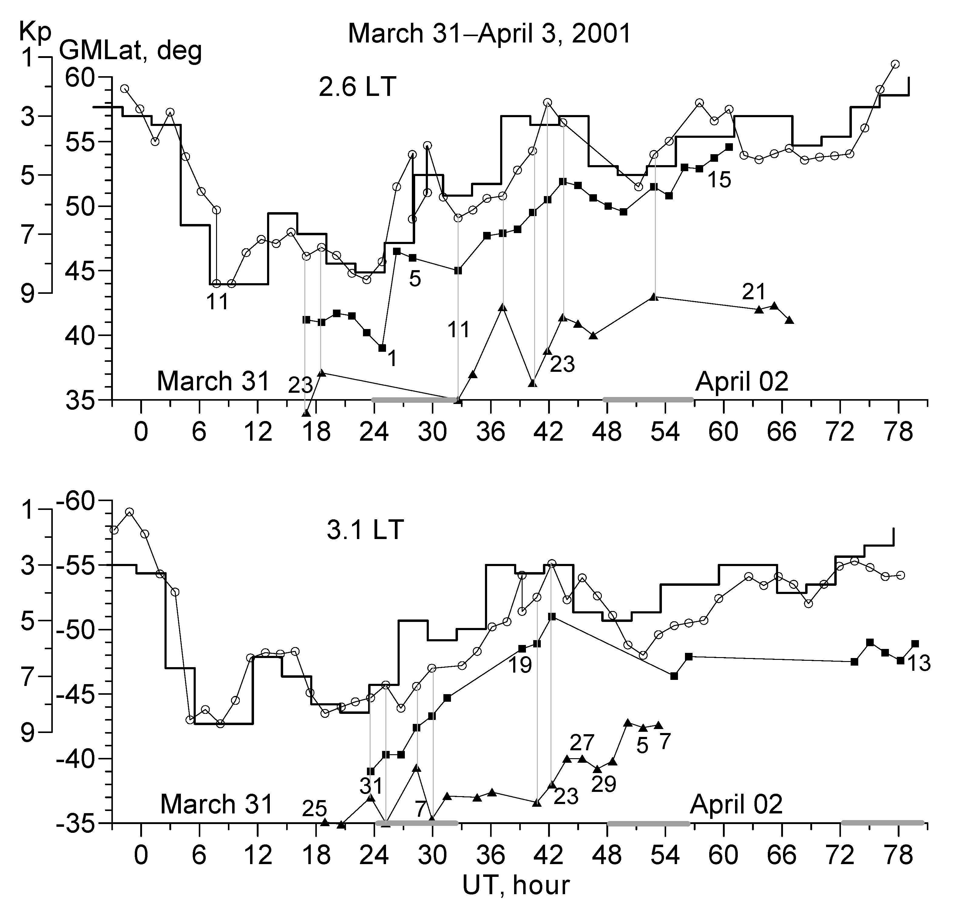
On 31 March–3 April 2001, the CHAMP satellite recorded the ionospheric response to the giant storm with Kp-index maximum of 9− and Dst minimum of −387 nT. Figure 1 shows variations in the trough positions for ~2.6 LT in the Northern hemisphere and ~3.1 LT in the Southern hemisphere. To facilitate the discussion, the time is counted from 00 UT on March 31. All events in this paper are considered in terms of the Kp-index, as variations in the MIT position are related to Kp variations, according to a model presented earlier [14]. This model determines the average position of the MIT for all longitudes with a given Kp value. Therefore, the Y-axis for the Kp-index, in both position and scale, is connected to variations in the trough position, according to this model. The asymmetry of the hemispheres is also taken into account: In the Southern hemisphere, the MIT is, on average, slightly more equatorward than in the Northern hemisphere [21]. For the event under discussion, this difference was ~2°. Deviations from the model are mainly determined by a longitudinal effect. The longitudinal effect pattern (which, in fact, is a model) in both hemispheres for any local time, for a fixed value of Kp = 2, has been given in [22]. However, as the character of the longitudinal effect varies during a storm, this model is generally only used for qualitative analysis. The longitudinal effect is most pronounced in the Southern hemisphere, where the MIT is located at higher latitudes at Asian longitudes and at lower latitudes at American longitudes [22]. As this is the case, when the storm began, at longitudes of 45–115°, the MIT was located at higher latitudes than in the model, and at lower latitudes at longitudes of 270–360° during the periods of 27–35 and 50–57 UT.
The variations in the Kp-index shown in Figure 1 are shifted to the right, as the delay in the MIT response in both hemispheres is 3.0–3.5 h. This delay time τ depends on the growth rate of geomagnetic activity and is determined by the formula τ = −0.4 + 4.3ΔKp/Δt [14]. This estimate of the trough response delay is used below, for all the storms considered. Note, however, that the correct determination of the delay time is possible only for storms with a relatively long main phase, as the 3-h Kp-index is quite a rough measure of geomagnetic activity. Considering this delay, it can be seen, from Figure 1, that variations in the MIT position (circles) clearly tracked the variations in the Kp-index. Note that, in the Northern hemisphere, a double trough was observed during sharp changes in the Kp-index after 06 UT and 27 UT (satellite passes 11 on 31 March and 5–7 on 1 April). This was probably due to the formation of a new trough while the old trough still existed. In the Southern hemisphere, a double trough was observed on pass 19 on 1 April. However, the cases of MIT bifurcation require separate analysis. It is also worth noting that, during the maximum perturbation, the MITs in both hemispheres were located at extremely low latitudes of 44° at 2.6 LT in the Northern hemisphere and −43° at 3.1 LT in the Southern hemisphere. The difference seems to be determined by the local time and hemispheric asymmetry.
The RIT (the squares in Figure 1) is usually located a few degrees equatorward of the MIT. During the storm under consideration, two trends have been observed in the RIT behavior: The RIT appears at the storm recovery phase each time after a local increase in geomagnetic activity and tends to longitudes with weak geomagnetic field (these longitudes are marked by thick lines on X axis in Figure 1). In the Northern hemisphere, the first trend is stronger while, in the Southern hemisphere, the second one prevails, such that it is difficult to give preference to one or another. The RIT in both hemispheres appeared at extremely low latitude of 39° (L ~ 1.66). The equatorward edge of the magnetospheric ring current during an extreme storm can shift to the same latitude of L ~ 1.6–1.7 [19]. By the end of the storm recovery phase, the RIT shifts to the typical latitudes of the residual ring current, 52–56° [20].
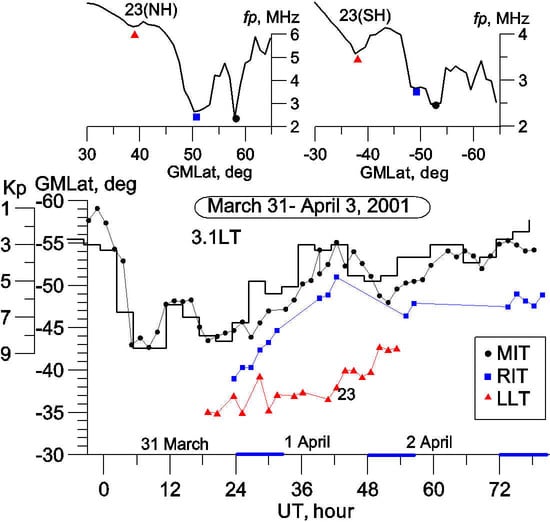
Figure 2 shows the latitudinal fp profiles. As the dynamics of the low-latitude trough (the triangles in Figure 1 and Figure 2) are of the greatest interest, the most typical LLT cases were selected for demonstration in Figure 2. The RIT, though, can also be clearly seen in Figure 2. In the Northern hemisphere, it was pronounced on passes 1 and 23 on 1 April, and pass 15 on 2 April. On pass 21 on 1 April, the RIT and MIT actually represent a joint structure. This is quite a typical situation [16]. In the Southern hemisphere, the RIT was most clearly separated from the MIT during pass 13 on 2 April. On pass 25 on 31 March, the fp minimum equatorward of the MIT is marked as the RIT, but this minimum was formed by only one fp value. Such cases would usually remain unidentified as troughs; therefore, this case in Figure 1 is not marked as the RIT. On pass 31 on 31 March, the structure at latitudes of 35–40° appears to be a joint trough, comprised of the RIT and LLT. The same can be said about the MIT and RIT during pass 23 on 1 April. It should be noted, in this regard, that the separation of the MIT and RIT is sometimes an ambiguous task. In a simple case, where the troughs are clearly separated, the MIT is determined in accordance with the model (Kp-index), and the RIT is several degrees equatorward. However, when they are located close to each other or merge into one, it is difficult to distinguish them. For example, it is difficult to say what kind of trough we were dealing with in the Northern hemisphere during the period 62–67 UT. In such cases, it seems that a joint MIT–RIT structure is involved. These uncertainties, however, do not fundamentally affect the analysis, as the latter is mainly based on clearly defined cases.
The low-latitude trough appeared after a local increase in geomagnetic activity on passes 23 in the Northern hemisphere and 25 in the Southern hemisphere. In the Northern hemisphere, the LLT was recorded at the lowest latitude of 34° (L = 1.46), while that in the Southern hemisphere was recorded at latitude of −35° (L = 1.5). These are the latitudes of the maximum of the inner radiation belt (L ~ 1.5). At the late stage of the recovery phase, the LLT disappears at latitudes of 42–43°. Figure 2 shows examples where the LLT is pronounced. The deepest trough was observed in the Southern hemisphere on passes 23, 27, and 29 on 1 April. In the Northern hemisphere, the LLT was manifested as a shallow minimum of electron density. This minimum is easy to miss in an analysis, which is probably why it had not been discovered earlier. To detect it, a detailed analysis of the dynamics in the structure of the entire ionosphere should be conducted. In addition, we need extreme storm data, as the LLT is generally not recorded in quiet conditions (at least, on a regular basis). The LLT location in both the Northern and Southern hemispheres is not related to the local longitude of observations. Cases of simultaneous observation of all three troughs are shown in Figure 2 by vertical lines. There were quite a few such cases in both hemispheres. There was a rather strong interhemispheric asymmetry for all three troughs, despite the close local time of measurements. The asymmetry in the MIT position was mainly related to the longitudinal effect. The asymmetry in the position and occurrence probability of the RIT and LLT is discussed below.
3.2. Storm of 31 March–1 April 2001. Day Conditions
In the daytime, all troughs were weakly expressed and were not always clearly revealed in the satellite data. This is due to the fact that any ionospheric plasma irregularities, including troughs, were filled by solar radiation during the day. Additionally, the RIT is formed by the precipitation of energetic ions from the asymmetric magnetospheric ring current, which is much more intense in the night sector than in the daytime one. During the event in question, the troughs were clearly visible only in the Southern hemisphere. Figure 3 shows variations in the trough positions in this hemisphere for ~14.3 LT. The MIT, as a rule, manifests itself as a shallow minimum of fp. Nevertheless, the MIT position was determined quite accurately; it also tracked variations in the Kp-index (with a delay of about 2.5 h), as at night. Variations in the Kp-index are related to variations in the dayside trough according to [21]. The trough moved equatorwards with an increase in geomagnetic activity at a rate of 1.7 Kp. The deviations from the model at the beginning of the storm were associated with a strong longitudinal effect.
The RIT appeared during the main phase of the storm and was clearly defined on pass 12, as shown by the fp profile in Figure 3 (on the right). On pass 14, all three troughs were revealed. At that point, the trough at lowest latitude of −47.4° was the most pronounced. The MIT was not defined clearly, as its polar wall was weakly expressed; but its minimum position was in good agreement with the model. The trough at the intermediate latitude of −56.7° can be easily overlooked in the analysis but, along with other troughs at typical latitudes of the residual ring current, it formed a separate branch of the trough. Only the MIT and RIT were recorded on passes 16–24, although the fp inflection at low latitudes could be associated with a weakly expressed LLT.
The appearance of the clearly defined low-latitude trough on passes 26, 28, and 30 was certainly associated with a local increase in geomagnetic activity during this period. On the other hand, they were still at longitudes of the American–Atlantic sector. On pass 28, one can see all three troughs again. All troughs were quite well-defined. The LLT was at latitude of −44.3° (L ~ 1.9), the lowest latitude for a dayside trough recorded by CHAMP data. During the storm recovery phase, neither the RIT nor MIT were recorded, as the electron density peak formed over a large belt of latitudes and filled both troughs. At the equatorward edge of this peak, there was a shallow minimum of electron density, which is not a trough. This minimum was evidently formed during the negative phase of the ionospheric storm, as can be seen from a comparison with pass 3 (dashed curve) recorded at the same longitude, but on a quiet day (30 March). All these minima are shown as the diamonds in Figure 3.
3.3. Storm of 5–7 November 2001
The CHAMP recorded the ionosphere response to another severe magnetic storm of 5–7 November 2001, when the Kp-index reached 9− and the Dst minimum was −272 nT. The most interesting manifestation of this storm was observed in the evening sector of the ionosphere in the Southern hemisphere. The variations in the trough positions for 18.5 LT are shown in Figure 4. The quality of the CHAMP data during this storm was worse than usual; however, this did not interfere with the analysis of the ionosphere structure. The storm pattern in the evening sector was quite simple. The MIT, in general, tracked the variation in the Kp-index without high delay, as the disturbance developed slowly. The RIT appeared during the main phase of the storm, at latitude of −47.5°. Once formed, the RIT was observed alone for a while. At the latitudes of the MIT model, a distinct trough was not detected, as passes 7 and 9 in Figure 4 (on the right) show. As the recovery phase of the storm developed, the RIT, as usual, shifted to the latitudes of the residual ring current, 53–55°. It was clearly expressed throughout the whole time, as shown on all passes in Figure 4 (on the right). The most interesting feature of the storm was the formation of a prominent structure at latitudes around 40° on pass 7. The Langmuir probe at these latitudes was certainly influenced by a strong interference, as significant variations in the electron density were observed. A deep trough at latitudes of 35–40°, however, was revealed very clearly. On the next pass (9), only a shallow minimum fp remained; this is also indicated in Figure 4 (on the left). Note that the RIT and LLT appeared during the storm maximum at longitudes with high values of the geomagnetic field. On pass 15, a peak of the electron density was recorded, which may also be part of the perturbed structure. On pass 17, the MIT can be clearly determined. The wide RIT, with irregular bottom, was located equatorward. Therefore, its position (in Figure 4 on the right), was at a latitude of 52°, which corresponds to the middle of the wide trough.
3.4. Storm of 20–21 August 2002
The storms discussed above were extremely strong. A question arises: Can a low-latitude trough develop during a less intense storm? To answer this question, the storm on 20–21 August 2002, with Kp-index maximum 6+ and the Dst minimum −106 nT, was considered. During this storm, the satellite was located in the sectors of 4.5 and 17.0 LT in the Northern hemisphere and 5.0 and 16.0 LT in the Southern hemisphere. The RIT was observed in all sectors of local time. The LLT was clearly recorded only in the 5.0 LT sector. This is why Figure 5 shows variations in the trough positions only in the morning sector in the Southern hemisphere. The storm had a clearly defined growth phase, which allows for accurate determination of the delay in the trough reaction, which was equal to 2 h. The squares in Figure 5 mark the cases that are clearly related to the RIT, as they were located at latitudes equatorward of the MIT model. The RIT was very clearly expressed on all these passes. The LLT appeared at an early stage of the storm recovery phase, again at longitudes with a weak geomagnetic field. It appeared very clearly on passes 3 and 5 at latitudes of −34° and −35° GMLat, respectively. Then, as the geomagnetic activity decreased, it shifted to higher latitudes; up to 46°. On passes 15 and 17, a complex structure was observed, in which three troughs can again be distinguished (see Figure 5, on the right). Thus, during a less intense storm, the LLT was clearly visible only in the morning sector and only in the Southern hemisphere, although the local time of observations in both hemispheres did not differ much.
3.5. Storm of 6–8 November 2000
Analysis of the variations in the ionospheric structure during geomagnetic storms is not a simple task, as can be seen from the previous considerations. It is not always possible to clearly identify the ionospheric troughs or to understand their dynamics. First, it is not always possible to separate the MIT and RIT. Second, when the electron density at high latitudes is irregular, the MIT can be confused with the high latitude trough (HLT), which is located inside the auroral oval [23]. Conversely, at low latitudes, structures that can be confused with the RIT (or, even, the LLT) are sometimes observed. An example of such a structure, according to CHAMP data, was observed during the storm of 6–8 November 2000, in the Southern summer hemisphere. The dynamics of the trough for this storm in the morning sector (3.8 LT) are shown in Figure 6. The storm was quite strong, with the Kp-index reaching 7. The disturbance developed slowly, such that the MIT responded to changes in the Kp-index with little delay.
At the beginning of the storm, the MIT was at lower latitudes than in the model, due to the longitudinal effect. There are no data for the first maximum of the storm while, during the second, the trough was formed at lower latitude than the model position and remained significantly equatorward during the recovery phase. Moreover, it appeared at longitudes with the weak magnetic field. This behavior is typical for the RIT. The latitudinal fp cross-section for pass 8 on 7 November is shown in Figure 6 (on the right). Both troughs, that is, the MIT and RIT, were simultaneously observed only during the late stage of the storm recovery phase. For example, they were clearly distinguished on pass 28. There was another increase in geomagnetic activity after 75 UT. With this enhancement, the formation of the structure shown on pass 12 on November 8 is apparently connected (Figure 6, on the right). It is quite similar to the trough but located at too low latitudes. This structure appeared at the longitudes of the American–Atlantic sector (the lowest-latitude examples belonged to the longitudes of 305–355°). Note the longitudes of the Weddell Sea Anomaly (WSA), which, in the Southern summer hemisphere at night, manifests itself as a strong increase in the electron density at high latitudes (see, e.g., [24]). The main reason for the WSA formation is a strong neutral wind directed to the equator [25]. This wind lifts the F2 layer up, reduces recombination, and increases foF2 accordingly. As a result, the sharp increase in the electron density filled both troughs, the MIT and RIT, and created an artificial minimum (pseudo-trough) at lower latitudes. This can be seen from the comparison of passes 28 on November 7 and 12 on November 8. After 81 UT, the geomagnetic activity decreases, wind velocity decreases, and the satellite appears at longitudes of the longitudinal effect maximum. As a result, on pass 20 (recorded at longitude of 150°), the trough was at latitude of −65.8°, that is, ~30° poleward of the electron density minimum on pass 10.
This structure, in the form of a well-defined trough equatorward of the WSA, has been previously described, according to DMSP data [26]. On 14 January 1997, under quiet night conditions, the trough was located at a minimum latitude of −42.4° GMLat. The authors called this trough “the heavy-ion stagnation trough” and associated it with the stagnation of ionospheric plasma within the horizontal drift and with the processes in the South Atlantic Magnetic Anomaly. All these reasons may contribute to the decrease in plasma density; however, it seems that the main reason is the increase in plasma density during the formation of WSA at high latitudes, which creates an artificial minimum at low latitudes.
4. Discussion
4.1. Trough Position Dependence on Kp-index
Figure 7 depicts the dependence on the Kp-index the position of the following structures: auroral oval, MIT, plasmapause, RIT, and LLT. The auroral oval and plasmapause positions were taken from [1,2]. The trough positions were revealed from the CHAMP data for all strong storms with Kpmax ranging from 5+ to 9−. The MIT was selected only at the same time as the RIT or LLT. The data were mainly obtained for after midnight/morning hours in both hemispheres (the data in the Southern hemisphere were taken with a positive sign). Three trough branches can be clearly distinguished: sub-auroral (i.e., MIT), mid-latitude (i.e., RIT), and low-latitude (i.e., LLT). The separation of the MIT and RIT was carried out while analyzing each case; this cannot be 100% unambiguous, as discussed above. This is especially true for Figure 7, where different cases are presented for different Kp-index values. Therefore, on the joint plot, the arrays of the MIT and RIT overlap. Nevertheless, both branches of the trough were determined quite confidently.
The MIT position dependence on the Kp-index in the post-midnight sector has the standard form: ΛMIT = 61.2°–2.0 Kp. The longitudinal variations and local time dependence were not been taken into account, which determines the relatively large standard deviation of σ = 2.6° and low correlation coefficient r = 0.82. The upper bold line presents the changes in the position of the equatorial border of the auroral oval at midnight. The approximating line is drawn through the extreme points of 66° for Kp = 0 and 48° for Kp = 9, as indicated in the Introduction. The approximating lines for the MIT and the auroral oval agree well, provided that the local time is different. Note that, according to [4], the MIT is usually located 2–5° equatorward of the auroral oval, which why it is a sub-auroral trough.
The RIT position dependence on the Kp-index is as follows: ΛRIT = 56.0°–1.8 Kp. The standard deviation is σ = ±2.8° and the correlation coefficient is r = 0.72, indicating that its dependence on the Kp-index is weaker. The dashed line approximates the plasmapause position, according to [1]. This corresponds to the plasmapause measurements for low Kp values and SAR-arc observations for high Kp values. The most studies have associated the plasmapause with the MIT, which is actually observed in Figure 7 for low Kp values. However, for high Kp values, the dashed line is closer to the RIT position. This is also correct, as the RIT and SAR-arc are formed by precipitation from the ring current. This precipitation is the most intense in the outer plasmasphere (i.e., a little equatorward of plasmapause). The low-latitude trough can also be quite clearly distinguished in Figure 7. Its position depends even more weakly on the Kp-index: ΛLLT = 43.3°–0.9 Kp (σ = 2.4°, r = 0.55). The LLT is located deep inside the plasmasphere. Thus, in our opinion, all the structures in Figure 7 are in good agreement with each other.
Thus, the MIT formed during a giant storm with Kp = 9− was observed at extremely low latitude of 44° at 2.6 LT in the Northern hemisphere and at −43° (L ~ 1.9) at 3.1 LT in the Southern hemisphere. The minimum latitude for the RIT was 39° (L ~ 1.65) at Kp = 8+ and 2.6 LT in the Northern hemisphere, and −39.5° at Kp = 8+ and 2.1 LT in the Southern hemisphere; 4–5° equatorward of the MIT. Finally, the LLT was recorded at lowest latitude of -33.5° (L ~ 1.44) at Kp = 8+ and 2.1 LT in the Southern hemisphere and at latitude of 34° (L ~ 1.46) at Kp = 8+ and 2.6 LT in the Northern hemisphere.
4.2. Trough Location Dependence on Longitude
The RIT is formed as a result of the precipitation of hot ions from the magnetospheric ring current, due to its decay during the recovery phase of the storm [16]. The ring current is located in the region of quasi-trapped particles; the lower the height of the mirror point in the atmosphere, the more intense the ion precipitation is. The mirror point height depends on the intensity, F, of the geomagnetic field. In turn, the value of F strongly depends on longitude; therefore, we can assume that the behavior of the RIT also depends on longitude. This fully applies to the LLT, which is undoubtedly formed by the precipitation of energetic particles from the inner radiation belt.
Figure 8 shows the variations in the RIT and LLT position with longitude in both hemispheres. The data are the same as in Figure 7; that is, for after midnight/morning conditions and for all Kp values. The cases of well-defined troughs at the early stage of the recovery phase are shown by filled symbols, while other cases are shown by empty ones. There were also longitudinal variations in the geomagnetic field magnitude, F, at the geomagnetic latitude of 45°. To complete the scheme, the variations in the MIT position [22] and in the position of the equatorward edge of the auroral oval (taken from [27,28]) are also presented. Both borders are defined for midnight.
During a geomagnetic storm, the strong asymmetric ring current is formed in the night sector of the magnetosphere. It mainly consists of ions with energies of 10–100 keV. During a severe storm, its equatorward edge reaches latitudes of L ~ 1.6–1.7 [19]. The RIT was observed (under high Kp values) at extremely low latitude of 39° (L ~ 1.65), which exactly corresponds to the equatorward edge of the ring current. During the storm recovery phase, the ion precipitation from the region of the residual ring current was observed, for a long time, at latitudes of 52.5–60° (L = 2.7–4.0) [20]. The RIT is most often observed in the latitude belt of 50–58°. Thus, we can define 58° as the upper limit of the RIT observation (under low Kp values). Thus, the latitude belt of RIT existence is limited to latitudes from 39° to 58°. These latitudes are marked by thick lines in Figure 8.
Figure 8 illustrates that, at the initial stage of the recovery phase in the Southern hemisphere, the RIT (filled squares) actually appears at longitudes with weak geomagnetic field. As the recovery phase develops, the RIT shifts to the latitudes of the residual ring current. In Figure 8, it is most often recorded at latitudes of 54–56°. The dependence on longitude remains when the geomagnetic activity decreases; the RIT (empty squares) is still more often observed at longitudes of the Western hemisphere. In the Northern hemisphere, the longitudes with weak geomagnetic field are almost the same as in the Southern hemisphere; however, the F intensity is much larger. Therefore, when oscillating along the magnetic field line and drifting around the Earth, all of the particles must be deposited in the Southern hemisphere at longitudes with low geomagnetic field magnitude [29]. Indeed, in the Northern hemisphere, the RIT is observed less frequently than in the Southern hemisphere. At the initial stage of the recovery phase, it has been observed only in the Eastern hemisphere, including at longitudes with high F values. At the late stage of the recovery phase, there is no clear dependence on longitude in the Northern hemisphere. In this regard, it should be noted that, in the same study [29], Berg reported that the intensity of proton fluxes in the Northern hemisphere was not directly related to local longitude; in addition, longitudinal variations decreased sharply with increasing geomagnetic activity.
The region of LLT existence, as follows from the analysis of severe storms, is limited to latitudes of 34–45° (L ~ 1.45–2.00). This is marked, in Figure 8, by thin lines. These latitudes refer to the region of the internal radiation belt (IRB). It is usually populated by trapped protons with energies of 20‒100 MeV and occupies the region just up to L ~ 2, with a maximum at L = 1.5. During a magnetic storm, the fluxes of energetic protons and electrons increase sharply (by 1–3 orders of magnitude) [30,31,32,33]. These fluxes are associated with the intense precipitation of energetic particles [34,35,36]. In addition to the direct ionization effect, enhanced particle precipitation causes an increase in the ionospheric conductivity at the heights of the E layer, as well as growth of the conductivity gradients and, as a result, the generation of strong local electric fields, which are capable of producing strong upward/downward drifts of highly ionized plasma [31,37,38]. These drifts can, obviously, create both peaks and troughs in ionization.
The mirror points for quasi-trapped particles of the IRB, as well as those of the ring current, depend on the magnitude of the geomagnetic field. They fall the lowest in the South Atlantic Magnetic Anomaly (SAMA) region. Accordingly, when particles drift around the Earth, the L-shell is rapidly emptied at the longitudes and latitudes of this anomaly. Therefore, most of the phenomena associated with the precipitation of energetic particles from the IRB: an increase in plasma density, temperature, atmospheric glows, and so on, are most frequently observed in the SAMA region. However, particle precipitation from radiation belts and related phenomena have also been recorded at other longitudes [39,40,41,42]. Figure 8 shows that neither in the Northern nor in the Southern hemisphere is there a clear dependence of the localization of the LLT upon longitude.
5. Conclusions
A detailed analysis of several strong geomagnetic storms allowed for the creation of a new comprehensive pattern of ionospheric trough dynamics. This, first of all, applies to the simultaneous co-existence of three troughs. This factor is the key in dividing the troughs into three branches: sub-auroral, mid-latitude, and low-latitude troughs. The MIT is a sub-auroral trough, being located 2–5° equatorward of the auroral oval [3]. This trough tracks (with a certain delay) variations in the Kp-index, according to the MIT model. The delay in the MIT response is determined by the rate of changes in geomagnetic activity: The greater the rate, the greater the delay. The lowest latitudes of 44° GMLat for the MIT was recorded during giant storm at 2.6 LT in the Northern hemisphere and of −43° GMLat at 3.1 LT in the Southern hemisphere.
The second trough, RIT, is located equatorward of MIT; as such, it is a mid-latitude trough. The RIT is usually formed at the initial stage of the storm recovery phase at latitudes of 39–45° while, during the late stage of the recovery phase, it tends to the latitudes of the residual ring current (52–56°). The RIT is most often formed in the midnight/morning ionosphere. It is more frequently observed in the Southern hemisphere than in the Northern hemisphere. Separating the MIT and RIT is often challenging, as there may be different options: Only one MIT or only one RIT, both troughs at the same time, or a joint structure. The separation is only unambiguous when the MIT and RIT are simultaneously observed and they are clearly divided. The most difficult case is when they are located close together, such that they merge into a joint structure. Additionally, pseudo-trough structures can form at low latitudes, which may be confused with the RIT. Thus, the separation of troughs is not always possible with 100% confidence. However, all of this is not critical for analyzing the RIT dynamics.
The third, the low-latitude trough is located at the latitudes of 34–45°, characteristic of the inner radiation belt (IRB). The LLT can generally be quite clearly separated from the RIT, as shown in Figure 7, both by position and by a weaker dependence on the Kp-index. However, the LLT may be confused with the RIT when the equatorward edge of the magnetospheric ring current is at L ≤ 2 and the RIT appears at the IRB latitudes; however, this can only happen during extreme storms.
The troughs differ greatly in occurrence probability: (i) The MIT is almost always observed at night in winter and equinox; (ii) the RIT is formed only during the recovery phase of the storm (substorm), although it sometimes exists for more than two days; (iii) and only individual cases of the LLT may be registered during a severe storm. The occurrence probabilities of the RIT and LLT depend on the longitude, due to changes in geomagnetic field intensity.
Funding
This research received no external funding.
Data Availability Statement
Data sharing is not applicable to this manuscript.
Acknowledgments
The author would like to thank sponsors and operators of the CHAMP mission; Deutsches Geo Forschungs Zentrum (GFZ) Potsdam and German Aerospace Center (DLR). The CHAMP data are available on the website: http://op.gfz-potsdam.de/champ.
Conflicts of Interest
The author declares no conflict of interest.
References
- Khorosheva, O.V. Magnetospheric disturbances and the associated dynamics of ionospheric electrojets, auroras, and plasmapause. Geomagn. Aeron. 1987, 27, 804–811. (In Russian) [Google Scholar]
- Khorosheva, O.V. Relation of geomagnetic disturbances to the dynamics of the magnetosphere and the parameters of the interplanetary medium. Geomagn. Aeron. 2007, 47, 543–547. [Google Scholar] [CrossRef]
- Gussenhofen, M.S.; Hardy, D.A.; Heinemann, N. Systematics of the equatorial diffuse auroral boundary. J. Geophys. Res. 1983, 88, 5692–5708. [Google Scholar] [CrossRef]
- Ahmed, M.; Sagalyn, R.C.; Wildman, P.J.L.; Burke, W.J. Topside ionospheric trough morphology: Occurrence frequency and diurnal, seasonal and altitude variations. J. Geophys. Res. 1979, 84, 489–498. [Google Scholar] [CrossRef]
- Yeh, H.-C.; Foster, J.C.; Rich, F.J.; Swider, W. Storm time electric field penetration observed at mid-latitude. J. Geophys. Res. 1991, 96, 5707–5721. [Google Scholar] [CrossRef]
- Hayakawa, M.; Tanaka, Y.; Ohtsu, J. Satellite and ground observations of magnetospheric VLF hiss associated with the severe magnetic storm on 25–27 May 1967. J. Geophys. Res. 1967, 80, 86–92. [Google Scholar] [CrossRef]
- Hikosaka, T. On the great enhancement of the line [OI] 6300 in the aurora at Niigata on 11 February 1958. Rep. Ionos. Res. Jpn. 1958, 12, 469–471. [Google Scholar]
- Shiokawa, K.; Ogawa, T.; Oya, H.; Rich, F.J.; Yumoto, K. A stable auroral red arc observed over Japan after an interval of very weak solar wind. J. Geophys. Res. 2001, 106, 26091–26101. [Google Scholar] [CrossRef]
- Hayakawa, H.; Ebihara, Y.; Hand, D.P.; Hayakawa, S.; Kumar, S.; Mukherjee, S.; Veenadhari, B. Low-latitude aurorae during the extreme space weather events in 1859. Astrophys. J. 2018. [Google Scholar] [CrossRef] [Green Version]
- Deminov, M.G.; Karpachev, A.T.; Morozova, L.P. Subauroral ionosphere in SUNDIAL period on June, 1987 on Cosmos-1809 satellite data. Geomagn. Aeron. 1992, 32, 54–58. (In Russian) [Google Scholar]
- Deminov, M.G.; Karpachev, A.T.; Afonin, V.V.; Annakuliev, S.K.; Shmilauer, Y. Dynamics of midlatitude ionospheric trough during storms 1. A qualitative picture. Geomagn. Aeron. 1995, 35, 54–59. [Google Scholar]
- Deminov, M.G.; Karpachev, A.T.; Annakuliev, S.K.; Afonin, V.V.; Smilauer, Y. Dynamics of the ionization troughs in the night-time subauroral F-region during geomagnetic storms. Adv. Space Res. 1996, 17, 141–145. [Google Scholar] [CrossRef]
- Deminov, M.G.; Karpachev, A.T.; Afonin, V.V.; Annakuliev, S.K. The dynamics of the mid-latitude trough during the storms: Recovery phase. Geomagn. Aeron. 1996, 35, 45–52. (In Russian) [Google Scholar]
- Karpachev, A.T.; Deminov, M.G.; Afonin, V.V. Model of the mid-latitude ionospheric trough on the base of Cosmos-900 and Intercosmos-19 satellites data. Adv. Space Res. 1996, 18, 221–230. [Google Scholar] [CrossRef]
- Karpachev, A.T. The characteristics of the ring ionospheric trough. Geomagn. Aeron. 2001, 41, 57–66. (In Russian) [Google Scholar]
- Karpachev, A.T. Dynamics of main and ring ionospheric troughs at the recovery phase of storms/substorms. J. Geophys. Res. 2020. [Google Scholar] [CrossRef]
- Pavlov, A.V. Mechanism of the electron density depletion in the SAR arc region. Ann. Geophys. 1996, 14, 211–221. [Google Scholar] [CrossRef]
- Norton, R.B.; Findlay, J.A. Electron density and temperature in the vicinity of the 29 September 1967 middle latitude red arc. Planet. Space Sci. 1969, 17, 1867–1877. [Google Scholar] [CrossRef]
- Hamilton, D.; Gloecler, G.; Ipavich, F.; Stüdemann, W.; Wilken, B.; Kremser, G. Ring current development during the great geomagnetic storm of February 1986. J. Geophys. Res. 1988, 93, 14343–14355. [Google Scholar] [CrossRef]
- Hultqvist, B. The ring current and particle precipitation near plasmapause. Ann. Geophys. 1975, 31, 111–126. [Google Scholar]
- Karpachev, A.T. Variations in the winter troughs’ position with local time, longitude, and solar activity in the Northern and Southern hemispheres. J. Geophys. Res. 2019, 124, 8039–8055. [Google Scholar] [CrossRef]
- Karpachev, A.T.; Klimenko, M.V.; Klimenko, V.V. Longitudinal variations of the ionospheric trough position. Adv. Space Res. 2018, 63, 950–966. [Google Scholar] [CrossRef]
- Grebowsky, J.M.; Tailor, H.A.; Lindsay, J.M. Location and source of ionospheric high latitude troughs. Planet. Space Sci. 1983, 31, 99–105. [Google Scholar] [CrossRef]
- Karpachev, A.T.; Gasilov, N.A.; Karpachev, O.A. Morphology and causes of the Weddell sea anomaly. Geomagn. Aeron. 2011, 51, 812–824. [Google Scholar] [CrossRef]
- Klimenko, V.V.; Klimenko, M.V.; Karpachev, A.T.; Ratovsky, K.G.; Stepanov, A.E. Spatial features of Weddell Sea and Yakutsk anomalies in foF2 diurnal variations during high solar activity periods: Interkosmos-19 satellite and ground-based ionosonde observations, IRI reproduction and GSM TIP model simulation. Adv. Space Res. 2015, 55, 2020–2032. [Google Scholar] [CrossRef]
- Horvath, I.; Lovell, B.C. Investigating the relationships among the South Atlantic Magnetic Anomaly, southern nighttime midlatitude trough, and nighttime Weddell Sea Anomaly during southern summer. J. Geophys. Res. 2009, 114, A02306. [Google Scholar] [CrossRef] [Green Version]
- Vorobjev, V.G.; Yagodkina, O.I. Seasonal and diurnal (UT) variation in the boundaries of the auroral precipitation and polar cup. Geomagn. Aeron. 2010, 50, 625–633. [Google Scholar] [CrossRef]
- Luan, X.; Wang, W.; Burns, A.; Solomon, S.; Zhang, Y.; Paxton, L.J.; Xu, J. Longitudinal variations of nighttime electron auroral precipitation in both the Northern and Southern hemispheres from the TIMED global ultraviolet imager. J. Geophys. Res. 2011, 116, A03302. [Google Scholar] [CrossRef] [Green Version]
- Berg, L.E.; Søraas, F. Observations suggesting weak pitch angle diffusion of protons. J. Geophys. Res. 1972, 77, 6708–6715. [Google Scholar] [CrossRef]
- Frank, L.A. On the extraterrestrial ring current during geomagnetic storms. J. Geophys. Res. 1967, 72, 3753–3767. [Google Scholar] [CrossRef]
- Dmitriev, A.V.; Yeh, H.-C. Storm-time ionization enhancements at the topside low-latitude ionosphere. Ann. Geophys. 2008, 26, 867–876. [Google Scholar] [CrossRef]
- Lazutin, L.L.; Logachev, Y.I.; Muravieva, E.A.; Petrov, V.L. Relaxation of electron and proton radiation belts of the Earth after strong magnetic storms. Cosm. Res. 2012, 50, 1–12. [Google Scholar] [CrossRef]
- Baker, D.N.; Erickson, P.J.; Fennell, J.F.; Foster, J.C.; Jaynes, A.N.; Verronen, P.T. Space weather effects in the Earth’s radiation belts. Space Sci. Rev. 2018, 214, 17. [Google Scholar] [CrossRef] [Green Version]
- Dmitriev, A.V.; Minaeva, Y.S.; Orlov, Y.V. Model of the slot region of Earth’s electron radiation belt depending on the heliospheric parameters. Adv. Space Res. 2000, 25, 2311–2314. [Google Scholar] [CrossRef]
- Panasyuk, M.I.; Kuznetsov, S.N.; Lazutin, L.L.; Avdyushin, S.I.; Alexeev, I.I.; Ammosov, P.P.; Antonova, A.E.; Baishev, D.G.; Belenkaya, E.S.; Beletsky, A.B.; et al. Magnetic storms in October 2003. Cosm. Res. 2004, 42, 489–534. [Google Scholar]
- Looper, M.D.; Blake, J.B.; Mewaldt, R.A. Response of the inner radiation belt to the violent Sun-Earth connection events of October–November 2003. Geophys. Res. Lett. 2005, 32, L03S06. [Google Scholar] [CrossRef] [Green Version]
- Lin, C.S.; Yeh, H.C. Satellite observations of electric fields in the South Atlantic anomaly region during the July 2000 magnetic storm. J. Geophys. Res. 2005, 110, A03305. [Google Scholar] [CrossRef] [Green Version]
- Foster, J.C.; Coster, A.J. Conjugate localized enhancement of total electron content at low latitudes in the American sector. J. Atmos. Sol. Terr. Phys. 2007, 69, 1241–1252. [Google Scholar] [CrossRef]
- Nagata, K.; Kohno, T.; Murakami, H.; Nakamoto, A.; Hasebe, N.; Kikuchi, J.; Doke, T. Electron (0.19–3.2 MeV) and proton (0.58–35 MeV) precipitations observed by OHZORA satellite at low zones L = 1.6–1.8. Planet. Space Sci. 1988, 36, 591–606. [Google Scholar] [CrossRef]
- Grachev, E.A.; Grigoryan, O.R.; Klimov, S.I.; Kudela, K.; Petrov, A.N.; Schwingenschuh, K.; Sheveleva, V.N.; Stetiarova, J. Altitude distribution analysis of electron fluxes at L = 1.2–1.8. Adv. Space Res. 2005, 36, 1992–1996. [Google Scholar] [CrossRef]
- Bogomolov, A.V.; Denisov, Y.I.; Kolesov, G.Y.; Kudryavtsev, M.I.; Logachev, Y.I.; Morozov, O.V.; Svertilov, S.I. Fluxes of quasi-trapped electrons with energies > 0.08 MeV in the near-Earth space on drift shells L < 2. Cosm. Res. 2005, 43, 307–313. [Google Scholar]
- Dmitriev, A.V.; Yeh, H.-C.; Panasyuk, M.I.; Galkin, V.I.; Garipov, G.K.; Khrenov, B.A.; Klimov, P.A.; Lazutin, L.L.; Myagkova, I.N.; Svertilov, S.I. Latitudinal profile of UV nightglow and electron precipitation. Planet. Space Sci. 2011, 59, 733–740. [Google Scholar] [CrossRef]
Figure 1.
The variations in the MIT (circles), RIT (squares), and LLT (triangles) position from 31 March to 3 April 2001, at 2.6 LT in the Northern hemisphere and 3.1 LT in the Southern hemisphere. Broken line depicts the Kp-index changes. Vertical lines indicate cases with three troughs. Horizontal thick line segments on the X-axis show longitudes with a weak geomagnetic field. The CHAMP passes under consideration are marked by the numbers. The time is counted from 00 UT on 31 March.

Figure 2.
Latitudinal fp profiles in the Northern and Southern hemispheres for the CHAMP passes indicated in Figure 1. The minimum of each trough is marked by corresponding symbol.
Figure 2.
Latitudinal fp profiles in the Northern and Southern hemispheres for the CHAMP passes indicated in Figure 1. The minimum of each trough is marked by corresponding symbol.

Figure 3.
The variations in the trough positions during 30 March–1 April 2001, in the Southern hemisphere at 14.3 LT. The designations are the same as in Figure 1. Thick vertical lines show the peaks of ionization, the diamonds mark the fp minima equatorward of this peaks. The time is counted from 06 UT on 30 March.

Figure 4.
The variations in the trough positions during 5–7 November 2001, in the Southern hemisphere at 18.5 LT. The designations are the same as in Figure 1. The time is counted from 09 UT on 5 November.
Figure 4.
The variations in the trough positions during 5–7 November 2001, in the Southern hemisphere at 18.5 LT. The designations are the same as in Figure 1. The time is counted from 09 UT on 5 November.

Figure 5.
Variations in the troughs position during the 20–21 August 2002, in the Southern hemisphere at 5.0 LT. The designations are the same as in Figure 1. The time is counted from 12 UT on 20 August.
Figure 5.
Variations in the troughs position during the 20–21 August 2002, in the Southern hemisphere at 5.0 LT. The designations are the same as in Figure 1. The time is counted from 12 UT on 20 August.

Figure 6.
The variations in the MIT (circles), RIT (squares), and pseudo-trough (diamonds) position during 6–8 November 2000, in the Southern hemisphere at 3.8 LT. Horizontal thick line segments show longitudes with a weak geomagnetic field. The CHAMP passes are marked by the numbers. The time is counted from 00 UT on 6 November.

Figure 7.
Dependence on the Kp-index the position of the structures, from top to bottom: auroral oval, MIT (circles and approximation line), plasmapause (dashed line), RIT (squares and line), and LLT (triangles and line). The CHAMP data refer to after midnight/morning conditions (00–07 LT).
Figure 7.
Dependence on the Kp-index the position of the structures, from top to bottom: auroral oval, MIT (circles and approximation line), plasmapause (dashed line), RIT (squares and line), and LLT (triangles and line). The CHAMP data refer to after midnight/morning conditions (00–07 LT).

Figure 8.
Scheme of localization of the auroral oval, MIT, RIT, and LLT in terms of longitude-latitude in the Northern and Southern hemispheres. The positions of the auroral oval and MIT are given for quiet (Kp = 2) midnight conditions. The RIT (squares) and LLT (triangles) data were obtained during geomagnetic storms in the interval from 00 to 07 LT. Filled and empty symbols correspond to large and low Kp values, respectively. Thick and thin horizontal lines limit the observation areas of RIT and LLT, respectively. F is geomagnetic field intensity.

Publisher’s Note: MDPI stays neutral with regard to jurisdictional claims in published maps and institutional affiliations. |
© 2021 by the author. Licensee MDPI, Basel, Switzerland. This article is an open access article distributed under the terms and conditions of the Creative Commons Attribution (CC BY) license (http://creativecommons.org/licenses/by/4.0/).
Share and Cite
MDPI and ACS Style
Karpachev, A. Sub-Auroral, Mid-Latitude, and Low-Latitude Troughs during Severe Geomagnetic Storms. Remote Sens. 2021, 13, 534. https://0-doi-org.brum.beds.ac.uk/10.3390/rs13030534
AMA Style
Karpachev A. Sub-Auroral, Mid-Latitude, and Low-Latitude Troughs during Severe Geomagnetic Storms. Remote Sensing. 2021; 13(3):534. https://0-doi-org.brum.beds.ac.uk/10.3390/rs13030534
Chicago/Turabian StyleKarpachev, Alexander. 2021. "Sub-Auroral, Mid-Latitude, and Low-Latitude Troughs during Severe Geomagnetic Storms" Remote Sensing 13, no. 3: 534. https://0-doi-org.brum.beds.ac.uk/10.3390/rs13030534
Note that from the first issue of 2016, this journal uses article numbers instead of page numbers. See further details here.