1. Introduction
With the continuous exploration into deep space and the increasing variety of electromagnetic applications, such as communication and navigation, monitoring and understanding of the solar-terrestrial space environment have become a hot field, including the Earth’s neutral atmosphere, ionosphere, plasmasphere, magnetosphere, and so on [
1]. The plasmasphere is a part of magnetosphere, also called the inner magnetosphere [
2], which starts from the top of the ionosphere and ends at the plasmapause. The plasmasphere is a donut-shaped region surrounding the Earth, containing the coldest plasma of the magnetosphere [
3]. It is currently believed that the charged particles in the plasmasphere mainly come from escape of the ionosphere and capture from the solar wind [
4,
5]. Richards et al. [
6] examined the relative importance of ionospheric and thermospheric densities and temperatures in producing the annual variation of the plasmaspheric electron density. Lee et al. [
7] compared the global plasmaspheric total electron content (TEC) with the ionospheric TEC simultaneously measured by Jason-1 satellite during the declining phase of solar cycle 23, and the results showed that the plasmaspheric density structures fundamentally followed the ionosphere, but there were still significant differences.
Radio signals are refracted by the charged particles, which affects satellite navigation, positioning and microwave remote sensing. When the navigation signals of Global Navigation Satellite System (GNSS) pass through the Earth’s ionosphere and plasmasphere, they are delayed due to the refraction. The magnitude of the impact is related to the total electron content (TEC) of the signal path [
8]. Although the electron density of the plasmasphere is much lower than that of the ionosphere, the region covered by the plasmasphere is dozens of times larger than that covered by the ionosphere. Therefore, the electron content of the plasmasphere accounts for a considerable proportion of the total electron content, which is usually about 10% in the daytime, but can reach 60% in the nighttime [
9,
10].
In some practical applications, for example, when using a single frequency GPS receiver for navigation and positioning, it is impossible to eliminate the effects of charged particles by ionosphere-free combined observations, while ionospheric empirical models are not precise enough to eliminate the error caused by such delay. Current main ionospheric models, such as the International Reference Ionosphere (IRI) model and the NeQuick model, can only estimate the electron content of the ionosphere, but ignore the plasmaspheric TEC (PTEC). Therefore, the corresponding delay effect cannot be estimated or corrected precisely, which has an impact on the final positioning results [
11,
12]. Therefore, it is important to estimate the PTEC for the delay correction. Furthermore, the coupling processes between the plasmasphere and the ionosphere are very complex. The studies on the plasmaspheric electron content variations and dynamic coupling processes between the plasmasphere and the ionosphere are crucial for understanding the plasmasphere [
13].
Before the advent of GNSS radio occultation technology, the PTEC was generally difficult to measure directly. The TEC acquired by ground GNSS receivers is the total electron content of the ionosphere and the plasmasphere. The ionospheric TEC (ITEC) can be obtained from the ionosonde or incoherent scattering radar (ISR), and then PTEC is indirectly calculated by subtracting ITEC from the total TEC [
14,
15]. However, there are a series of problems with these methods. Firstly, normally the electron density profile below the peak value of F2 layer can be obtained by the ionosonde, and the electron density profile above the peak value is extrapolated by the Chapman function [
16]. Secondly, the number of observation stations of ionosonde and ISR is relatively small, and the distribution is very sparse. In addition, the cost is a little high, which leads to limited coverages in the global ionospheric observations. Furthermore, there are likely systematic deviations between different observation techniques and methods, which will be involved into the PTEC estimation. Therefore, it is challenging to accurately estimate PTEC and establish the plasmaspheric model.
Nowadays, with the increasing number of GNSS Radio Occultation observations on Low Earth Orbit (LEO) satellites, the topside GNSS observations on LEO satellites provide a unique opportunity to directly estimate PTEC and study its variations in the plasmasphere, particularly Constellation Observing System for Meteorology, Ionosphere, and Climate (COSMIC) with six LEO satellites. The COSMIC can provide more than 2500 occultation events per day during the normal operation period of six LEO satellites [
17,
18]. In this paper, the PTEC is estimated, and its long-term variations are studied based on topside GPS observations on COSMIC with providing the slant TEC (sTEC) of the signal path. The sTEC is transformed into vertical TEC (vTEC) by a mapping function, and then the grid model of PTEC is established. The spatial and temporal distribution characteristics of PTEC are analyzed as well as its long-time variation characteristics from January 2007 to December 2017. In
Section 2, the data and method are introduced, the results and analysis are presented in
Section 3, and finally, conclusions are given in
Section 4.
2. Data and Method
The data used in this paper are the precise podTec provided by COSMIC from January 2007 to December 2017, which can be obtained from the COSMIC data analysis and archiving center (
https://www.cosmoc.ucar.edu/cdaac/). The PodTec files provide UTC time, three-dimensional coordinates of LEO and GPS satellites, observation elevation of the GPS-LEO observation link at LEO satellite, and the slant TEC on the signal path. It is worth noting that the hardware delays of the transmitters on GPS satellites and the receivers on COSMIC satellites have been deducted from the TEC, and the sampling rate of the observations is 1 s [
19]. Since the volume of observation data after 2017 is too small, we only use the observation data from 2007 to 2017 in this paper. In addition, to ensure the consistency of the altitude region covered by the observations, the observation data before LEO satellites lifting their orbits are also eliminated.
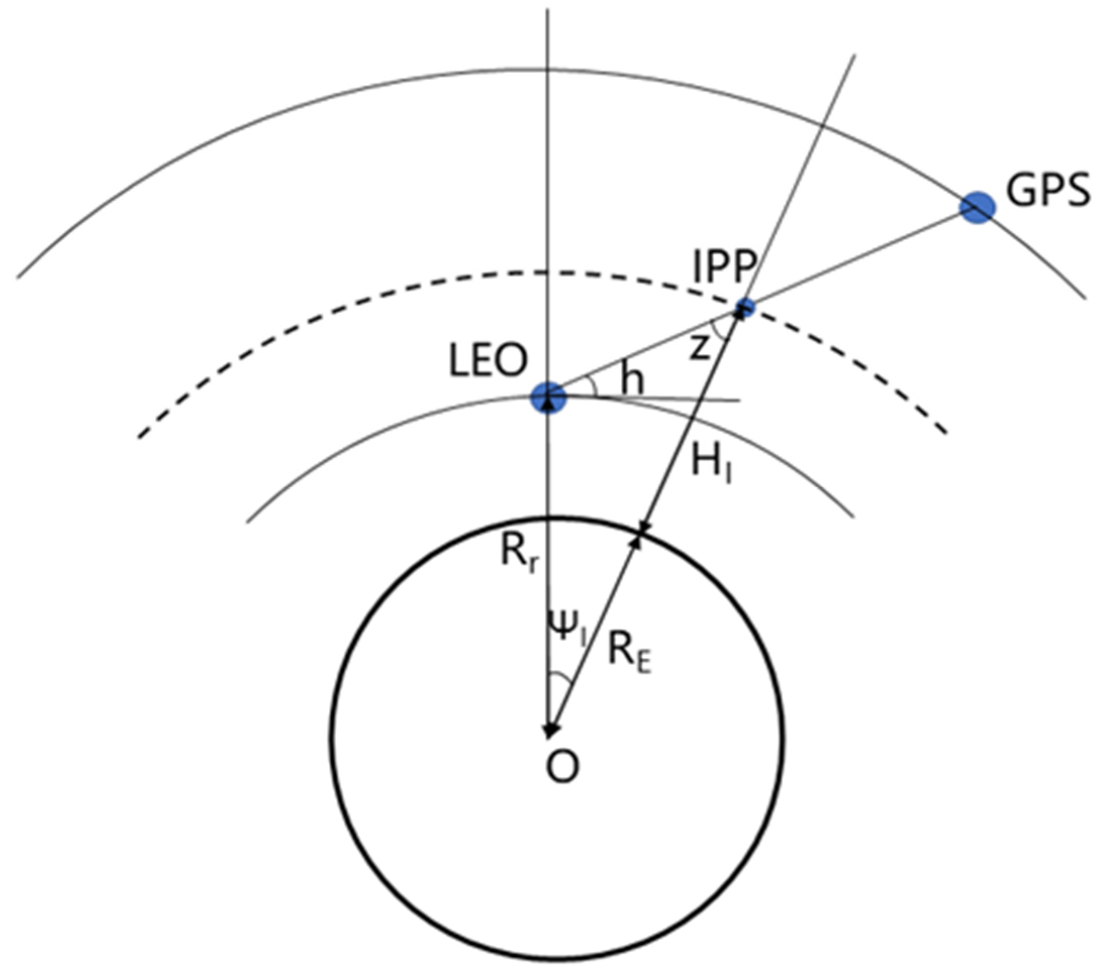
To estimate the plasmaspheric TEC, it is necessary to set a thin shell, and the electron content is assumed to be concentrated on the shell. The method of the gridded plasmaspheric TEC model is basically the same as that of the Global Ionosphere Model (GIM) [
20,
21]. We tested the effects of the thin shell heights on PTEC results, and found a small difference and little effect on the temporal and spatial distribution of PTEC. Therefore, we set the altitude of the thin shell at 1400 km. Detailed plasmaspheric TEC modeling is shown in
Figure 1.
Firstly, the baseline between the LEO and GPS satellites is transformed to the station-centered coordinate system, and then the azimuth angle
and the elevation angle
are calculated as:
where
and
are the geographic latitude and longitude of the LEO satellite, respectively, and
and
are the coordinates of the LEO-GPS baseline in Earth-centered Earth-fixed (ECEF) coordinate system and the station-centered coordinate system, respectively.
To reduce the mapping errors and multipath effects, only the observations with an elevation angle greater than 40° are used to establish the plasmaspheric TEC grid model. The sTEC observations with negative values or over 100 TECU, which can be considered to be unreasonable observations, are also removed. Then, we calculate the obliquity factor
between LEO and GPS satellites and the vertical TEC:
where
is the distance between the receiver on the LEO satellite and the Earth’s center,
is the radius of the Earth,
is the altitude of the single layer plasmasphere (here we set it as 1400 km). Then, the geographic longitude and latitude of the plasmaspheric piercing point can be calculated as follows:
where
is the geocentric angle between LEO satellite and the piercing point, and
and
are the geographic latitude and longitude of the piercing point, respectively.
The geographic longitude and latitude are converted to geomagnetic longitude and latitude, and the magnetic local time is calculated as follows:
where
and
are the geomagnetic latitude and longitude of the piercing point, respectively,
and
are the geographic latitude and longitude of the geomagnetic north pole, respectively, and
, and
,
and
are the universal time and magnetic local time of the observation, respectively.
Finally, we divide all the observations in a month or a season into groups with a latitudinal resolution of 2.5° and a temporal resolution of 20 min, and the observations in each group are weighted and averaged according to the value of as the PTEC of the corresponding grid point. In all the formulas above, angles are in radians and distances are in kilometers.
3. Results and Analysis
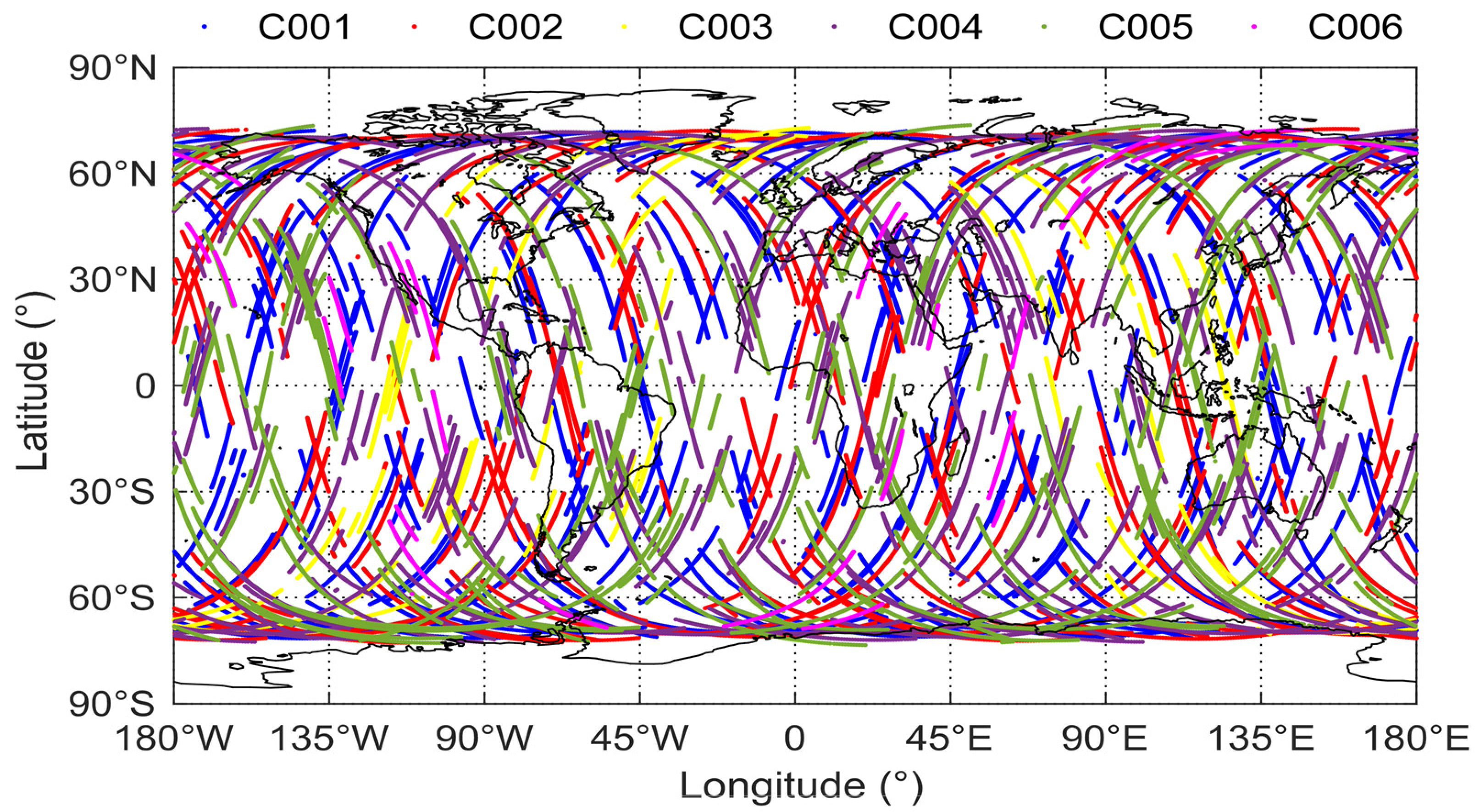
The COSMIC constellation consists of six LEO satellites, which provide dense global coverage plamaspheric observations.
Figure 2 shows the geographical distribution of the piercing points on the 1400 km thin shell on 2 January 2008. Due to the inclination of the satellite orbits and the lowest observation elevation angle of 40°, the distribution of the piercing points has gaps at the north and south poles. However, in the region between 72°S and 72°N, the topside observations of LEO satellites are well-distributed, and all observations can be regarded as observations from GPS satellite altitude (about 20,200 km) to COSMIC satellite altitude (about 800 km). Although this altitude range is not exactly consistent with the real plasmasphere, the observations are homogeneous in the detection altitude, and basically contain most of the charged particles of the plasmasphere, so they can be regarded as the observations for the plasmasphere. These conditions are quite favorable for plasmaspheric modeling.
3.1. PTEC Estimation from COSMIC
According to the definition of plasmasphere, the distribution of charged particles is dominated by the Earth’s magnetic field. Therefore, the geomagnetic coordinate system is used in modeling. The magnitude of PTEC is closely related to the position of the sun, so the geomagnetic longitude is converted to the magnetic local time. On the basis of topside GPS observations of COSMIC, the plasmaspheric TEC grid model is estimated. This paper mainly analyzes the temporal and spatial distribution and long-term variation of PTEC, considering the volume of data and the convenience of analysis, so we divide the observations separately by month and model. In this way, the effects of long-period variations like solar activity on PTEC are preserved, while the influence of geomagnetic activities, such as magnetic storms and sub-magnetic storms, which are relatively short-lived (from a few hours to one or two days), is averaged over one month’s observations, with a minimal impact on modeling. When analyzing the seasonal variation of PTEC, we combine the observations of three months together and re-weight the observations to calculate the PTEC.
The Global Core Plasma Model (GCPM) is the first real global plasmaspheric model, and was established by Gallagher et al. [
22] by integrating density distribution models of different regions. It covers the ionosphere, plasmasphere, plasmapause, plasmaspheric poles, and so on. In the ionosphere, GCPM adopts the international reference ionosphere model IRI. The plasmaspheric region is based on the density distribution model of H+ established according to the observations of DE-1 satellite by Gallagher et al. [
22]. The Persoon model is adopted in the polar regions [
23]. These regional models are integrated by mathematical fitting to create a static three-dimensional plasmaspheric model GCPM, which can extend from the ionosphere to 8 to 9 radii of the Earth.
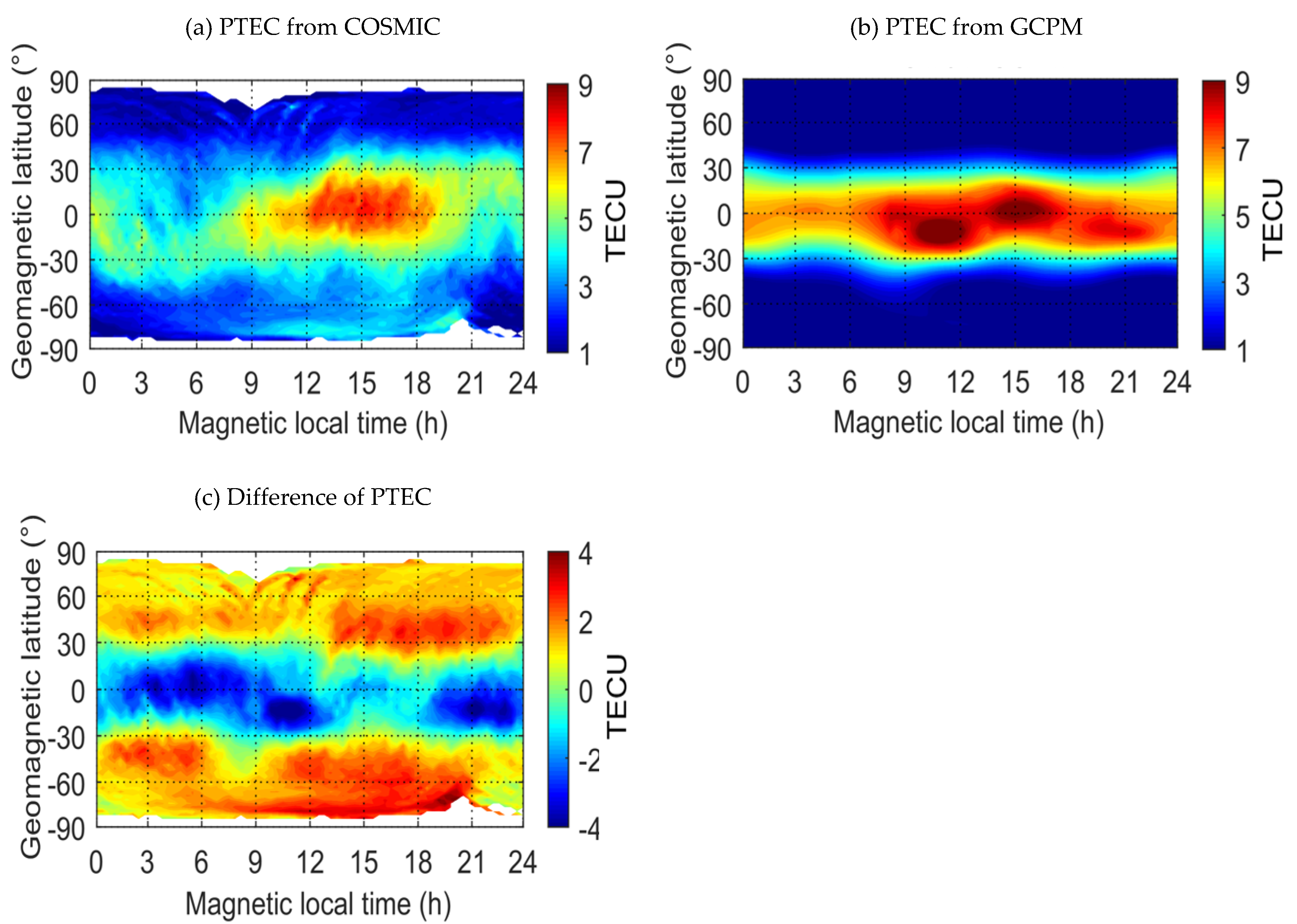
Figure 3 shows the comparison of PTEC from the topside GPS observations of COSMIC in January 2008 with the GCPM and the differences in the bottom panel. The blank regions in the top and bottom panels are caused by the fact that the observations of COSMIC cannot completely cover the polar region. In January 2008, the state of solar activity was quiet, and the F10.7 indices exhibit little change, at less than 80 sfu. This that the observations of PTEC from COSMIC and GCPM are almost consistent with respect to the overall characteristics. There is a significant belt with higher values of PTEC at geomagnetic latitudes between −45° and 45°, and PTEC values in the daytime are higher than those in the nighttime. In addition, the PTEC values in the top panel decrease slowly from the geomagnetic equatorial region to the geomagnetic polar regions, while in the middle panel, the PTEC values decrease rapidly in the geomagnetic middle-latitude regions. As a result, the differences show significant zonal belt distribution in the bottom panel, and in the middle and high geomagnetic latitudinal regions.
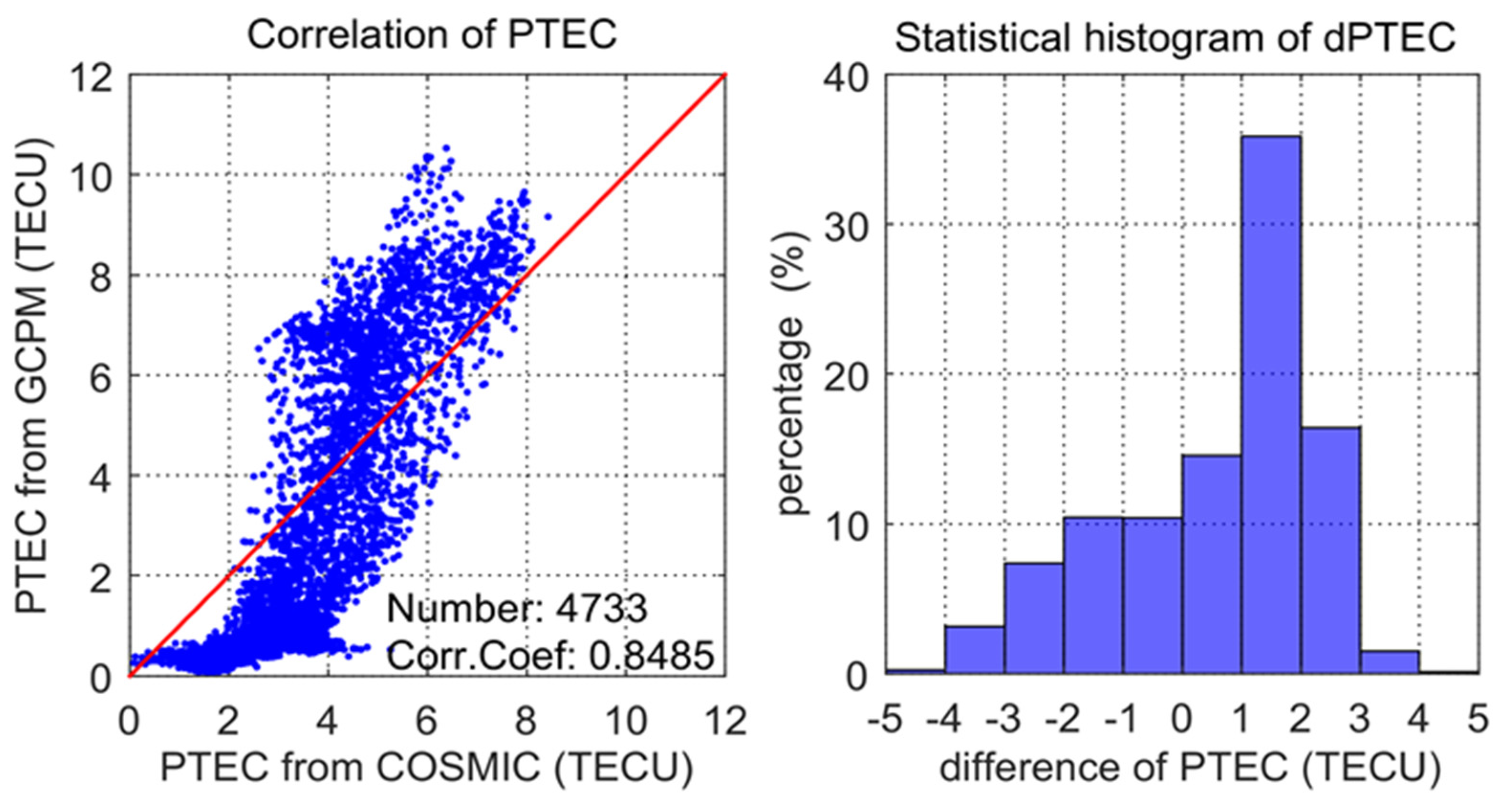
The left panel in
Figure 4 shows the comparison of the PTEC values from topside GPS observations of COSMIC and GCPM in January 2008 at corresponding positions. The correlation coefficient of PTEC values is 0.85, which indicates a good consistency between the PTEC from COSMIC observations and GCPM. The right panel shows the distribution histogram of PTEC differences. Almost all the differences are within ±4 TECU, and the numbers of differences over ±3 TECU are less than 5% of the total statistics, which also shows that the two PTEC results are in good agreement with each other.
In general, it has a relatively high correlation of PTEC between GCPM and the COSMIC observations, and the correlation is higher in quiet period of solar activity. However, since GCPM is a model fitted by mathematical formulas, the result is very smooth in numerical value and therefore the details cannot be seen from the model. The PTEC estimation from topside GPS observations of COSMIC is based on the actual observations, which contains more rich details.
3.2. Temporal-Spatial Distribution Characteristics of PTEC
The long-term variations of plasmaspheric TEC and its temporal-spatial distribution characteristics are analyzed using COSMIC-derived PTEC. According to the solar activity, we selected 2008 and 2014 as the representatives of low and high solar activity years, respectively, and established the PTEC gridded model using COSMIC observations by month and season, and the monthly and seasonal variations characteristics of PTEC under different states of solar activity are analyzed.
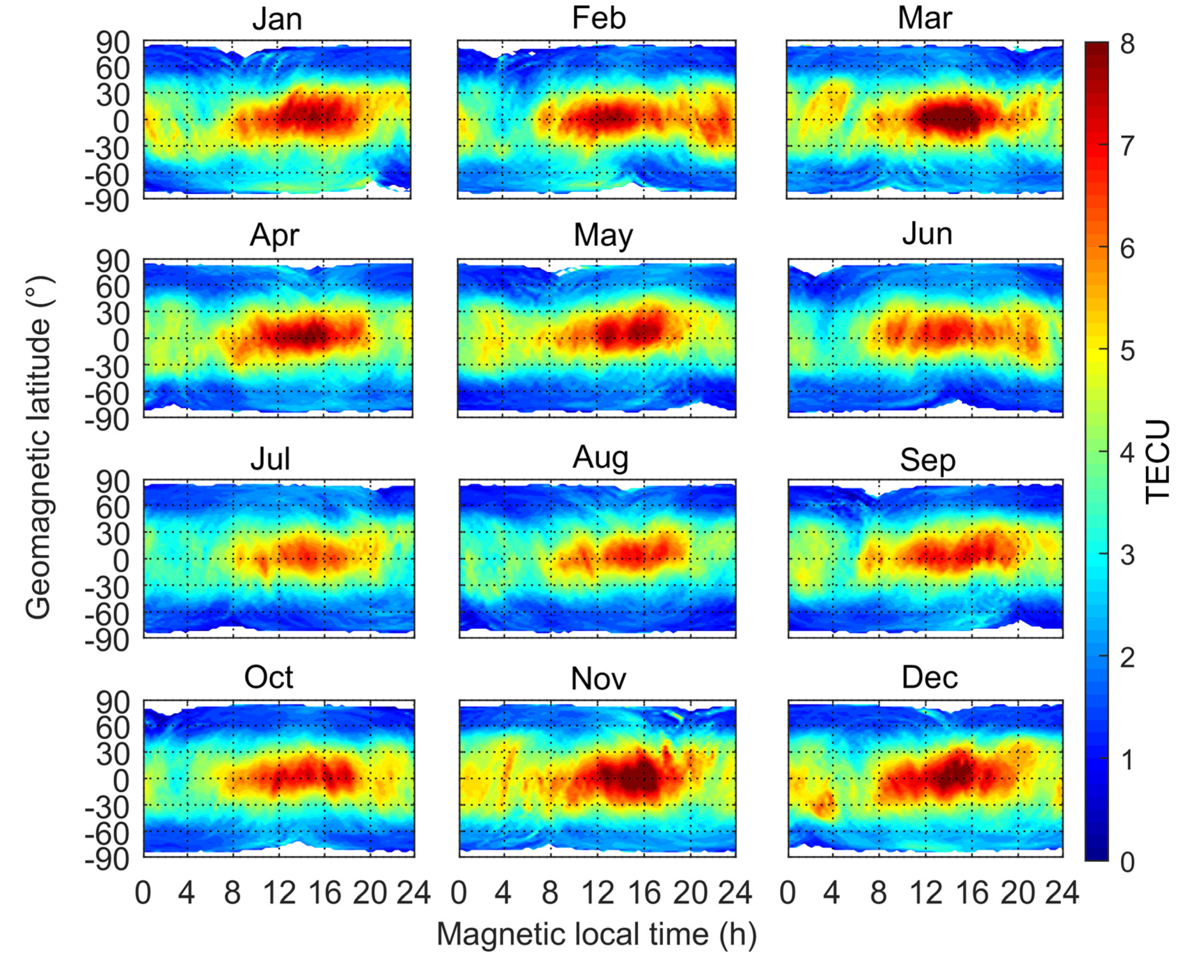
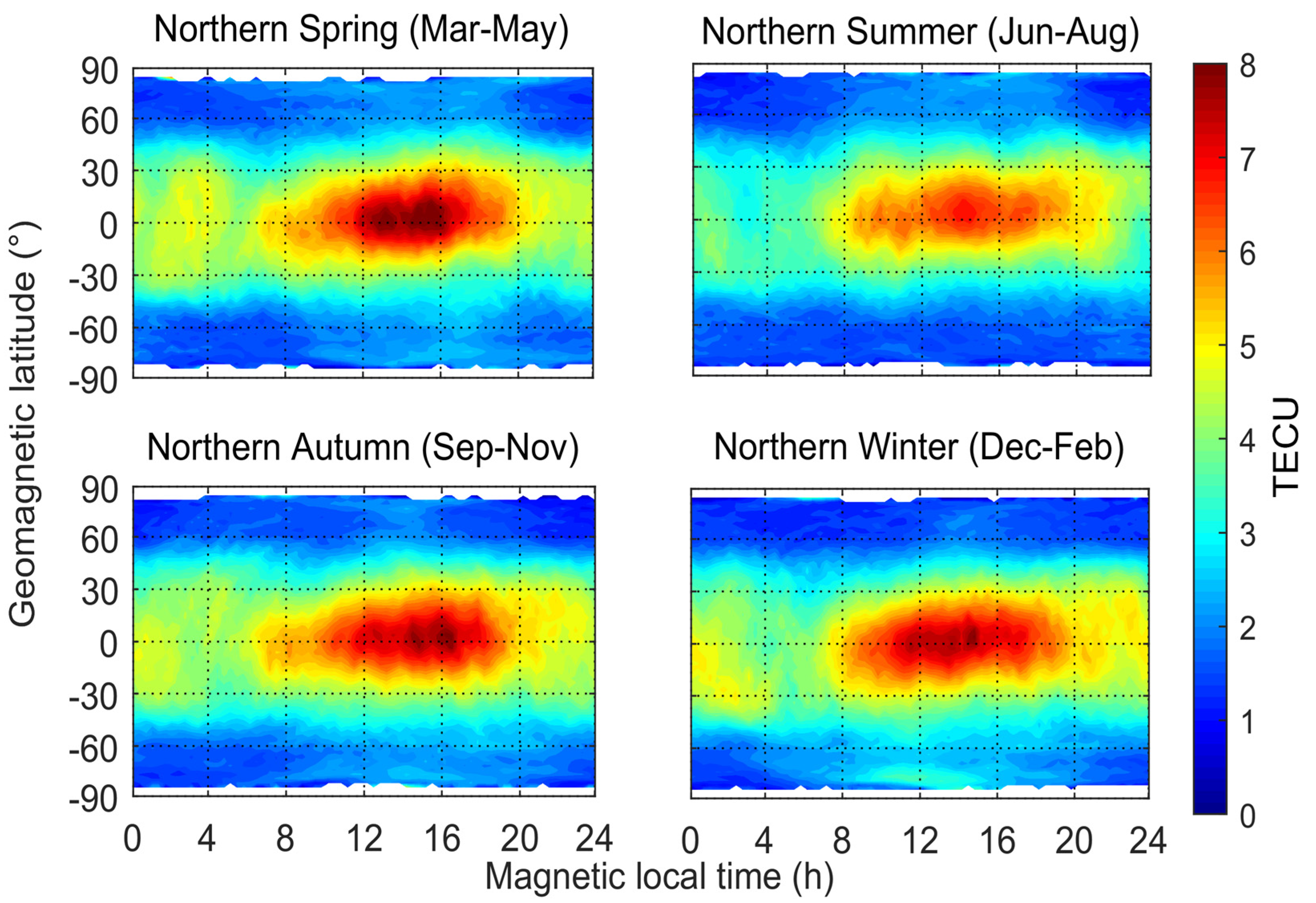
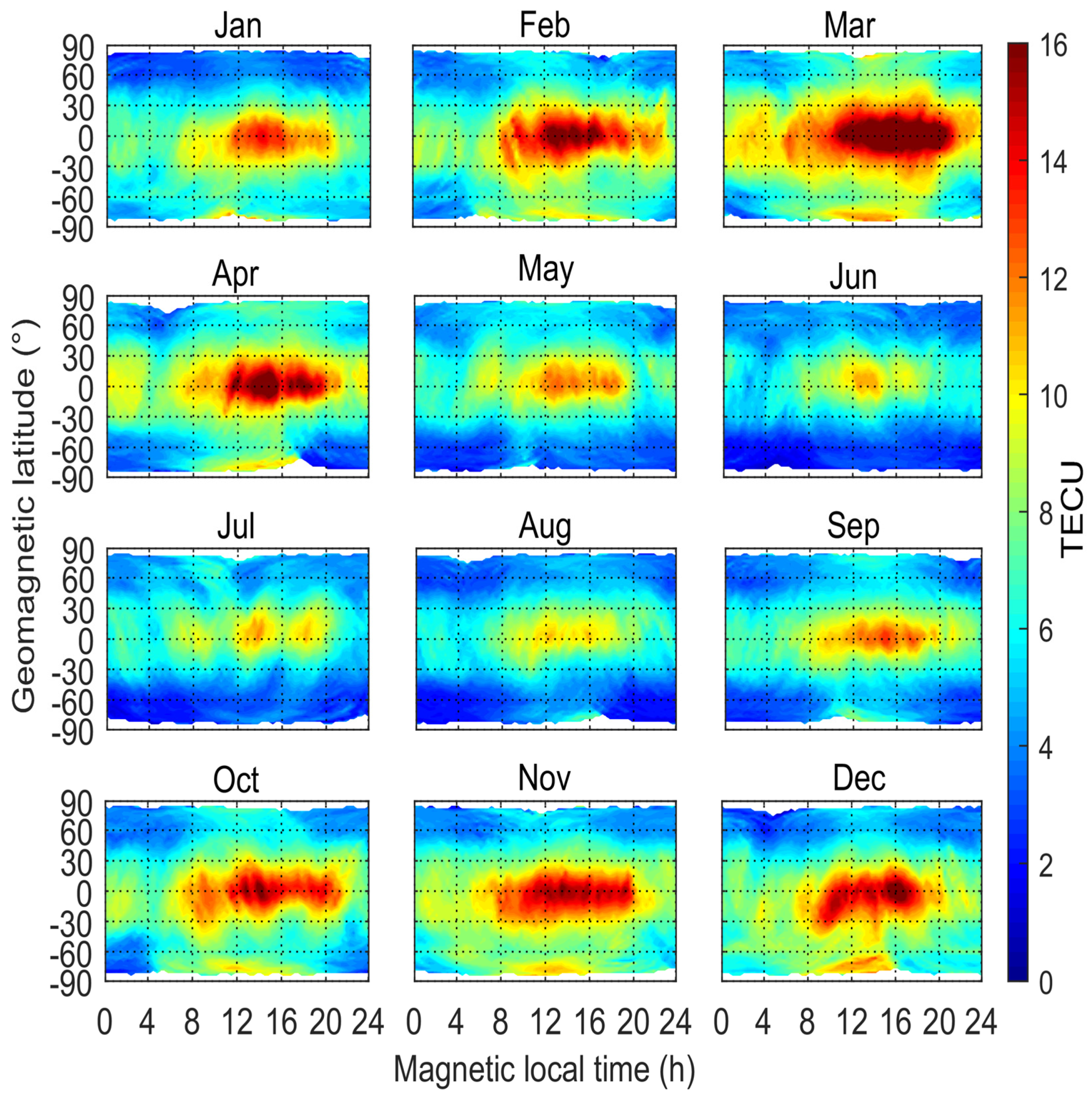
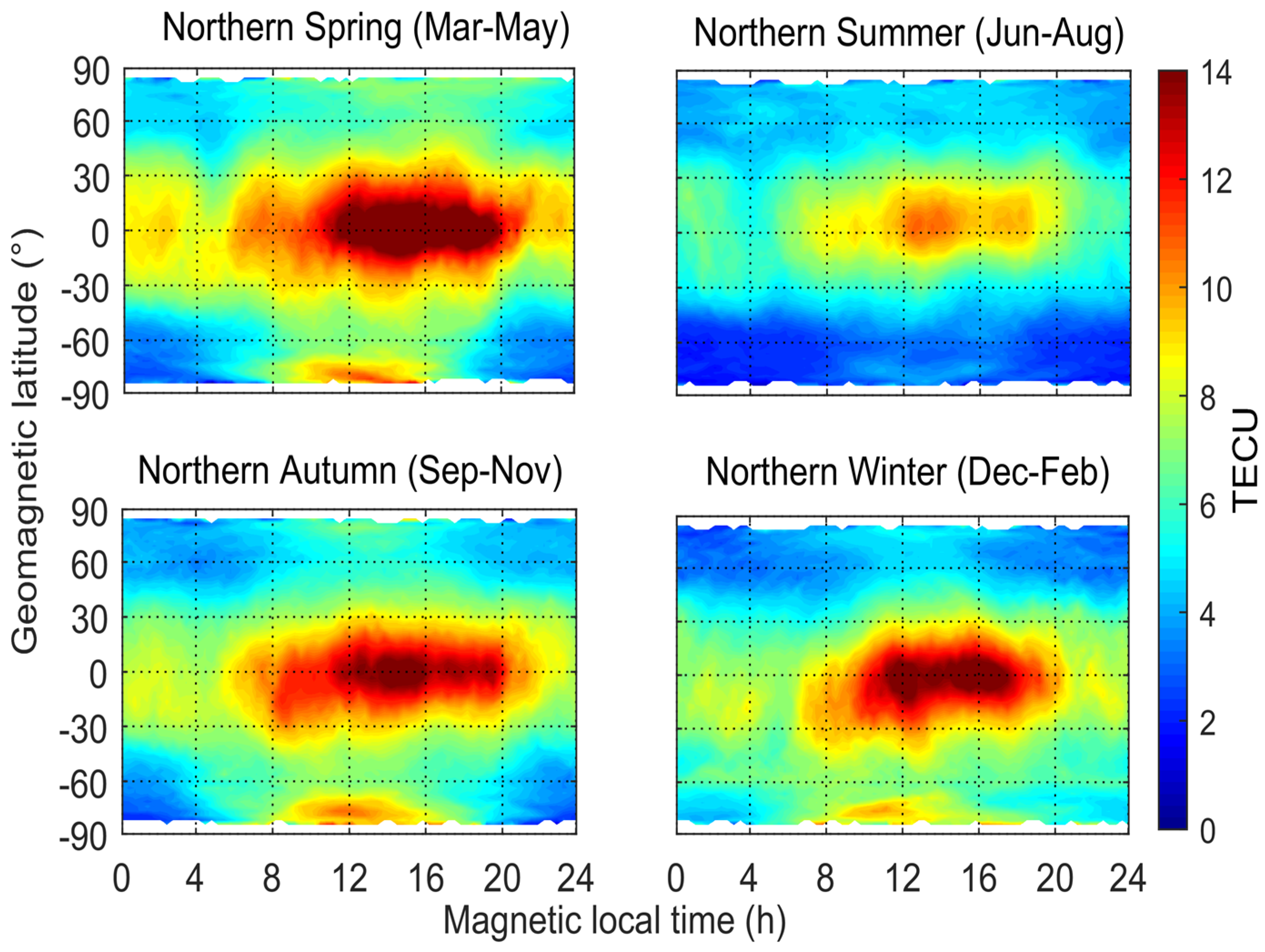
Figure 5 and
Figure 6 show monthly and seasonal variations of plasmaspheric TEC in 2008, respectively. Observations of January and February 2009 were also used in the subgraph in the bottom right panel of
Figure 6. The PTEC values in different months or seasons have the same following basic characteristics: PTEC values at daytime are higher than those at nighttime; PTEC values in lower geomagnetic latitudinal regions are higher than those in higher geomagnetic latitudinal regions; and there are obvious zonal belts with higher PTEC values within the ±45° geomagnetic latitudinal region. This is because the solar incidence angle in the geomagnetic low-latitude region is the greatest in the daytime, where the plasmasphere captures the most energy, and thus generates more charged particles through ionization. These phenomena can also prove a close relationship between the plasmaspheric TEC and solar activity, which will be analyzed in the next section.
In the high PTEC value belts within ±45° geomagnetic latitude, the peak values of PTEC in monthly and seasonal models all appear in the geomagnetic equatorial region between 14:00 to 17:00 o’clock in the magnetic local time, while the minimum values of PTEC appear between 3:00 and 6:00 o’clock in the magnetic local time. This can be explained by the coupling process between the plasmasphere and the ionosphere. The charged particles in the ionosphere drift upward along the Earth’s magnetic field lines to the plasmasphere in the daytime, while the charged particles in the plasmasphere will return to the ionosphere to maintain the electron density of the F layer in the nighttime, so the electron content of plasmasphere will reach the minimum value before sunrise [
24]. In
Figure 5, we can see that values of plasmaspheric TEC in June, July and August 2008 are significantly lower than those in other months, and values of plasmaspheric TEC in March and November are the highest. At the seasonal scale, the plasmaspheric TEC is the highest in the northern hemisphere spring and the lowest in northern summer, which are related to the variation of the vertical radiation region of the sun. The seasonal variation of the plasmaspheric TEC is consistent with the variation of the ionospheric TEC due to the strong coupling interaction [
25].
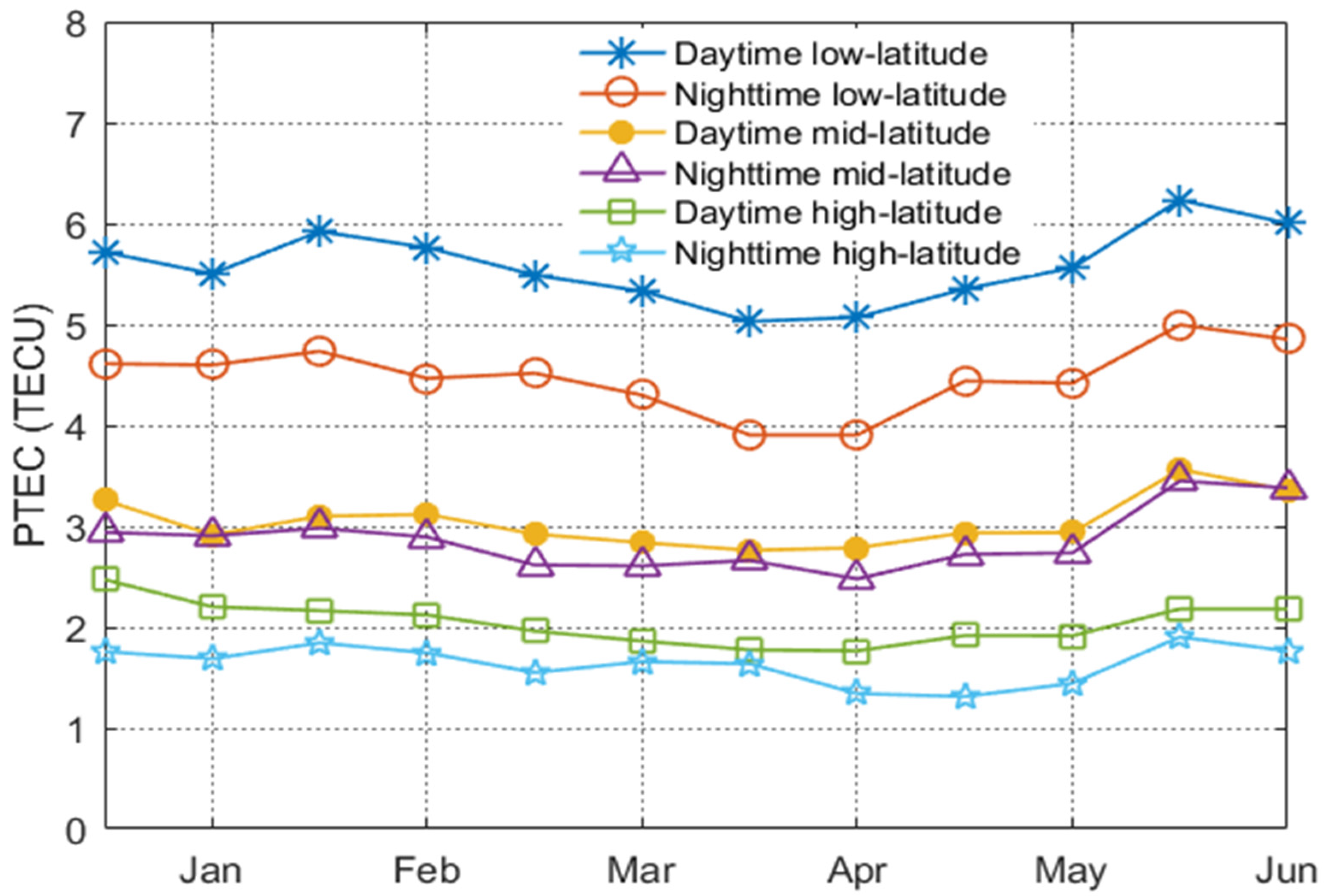
To analyze the influence of magnetic local time and geomagnetic latitude on plasmaspheric TEC, we divided the monthly PTEC into six parts. There are daytime and nighttime regions: the magnetic local time from 6:00 to 18:00 o’clock is the daytime, and the nighttime is from 18:00 to the second day’s 6:00 o’clock. As for geomagnetic latitude, it is divided into low-latitude, mid-latitude and high-latitude, with boundaries of ±30° and ±60°. The average PTEC of each region was calculated, and is shown in
Figure 7. Since the solar and geomagnetic activities were quite calm in 2008, the variations of plasmaspheric TEC in different regions were also small and gentle, with a maximum variation range of about 1.2 TECU. Apparently, the maximum values of plasmaspheric TEC always appeared in the low-latitude region in the daytime, and the maximum value was in November 2008, reaching 6.2 TECU. The sub-maximum values were in the nighttime low-latitude region, with a maximum value of 5 TECU in November. The differences between daytime and nighttime PTEC in the low-latitude region are about 1 TECU. In mid-latitude region, the plasmaspheric TEC is around 3 TECU, and there is a small difference between daytime and nighttime. However, the relative differences of plasmaspheric TEC between daytime and nighttime are quite large for the small value of PTEC in high-latitude region. In general, the effect of geomagnetic latitude on plasmaspheric TEC is more obvious.
Figure 8 and
Figure 9 show the monthly and seasonal variations of plasmaspheric TEC in 2014, respectively. Observations of January and February 2015 are also used in in the subgraph at bottom right of
Figure 9. The basic distribution characteristics of plasmaspheric TEC mentioned above still exist. The most obvious difference is that the belts with higher PTEC values are wider during the solar active period, especially in the daytime, which indicates that during the solar active period, a larger region of the plasmasphere can receive strong solar radiation, thus ionizing to generate more charged particles. In terms of numerical value, the peak values of PTEC are significantly higher than those in 2008, which are almost double in some months. In June, July and August 2014, the values of plasmaspheric TEC are smaller than those in other months, which is the same as 2008. This phenomenon is also reflected on the seasonal scale, whereby the values of plasmaspheric TEC in northern summer are much lower than those in other seasons. An interesting phenomenon is that the local maximum values of PTEC appear around 12:00 o’clock in the region of geomagnetic latitude -80° in spring, autumn and winter of the northern hemisphere, which indicates that the charged particles of the plasmasphere will accumulate in this region at noon, and its physical mechanism needs to be further studied.
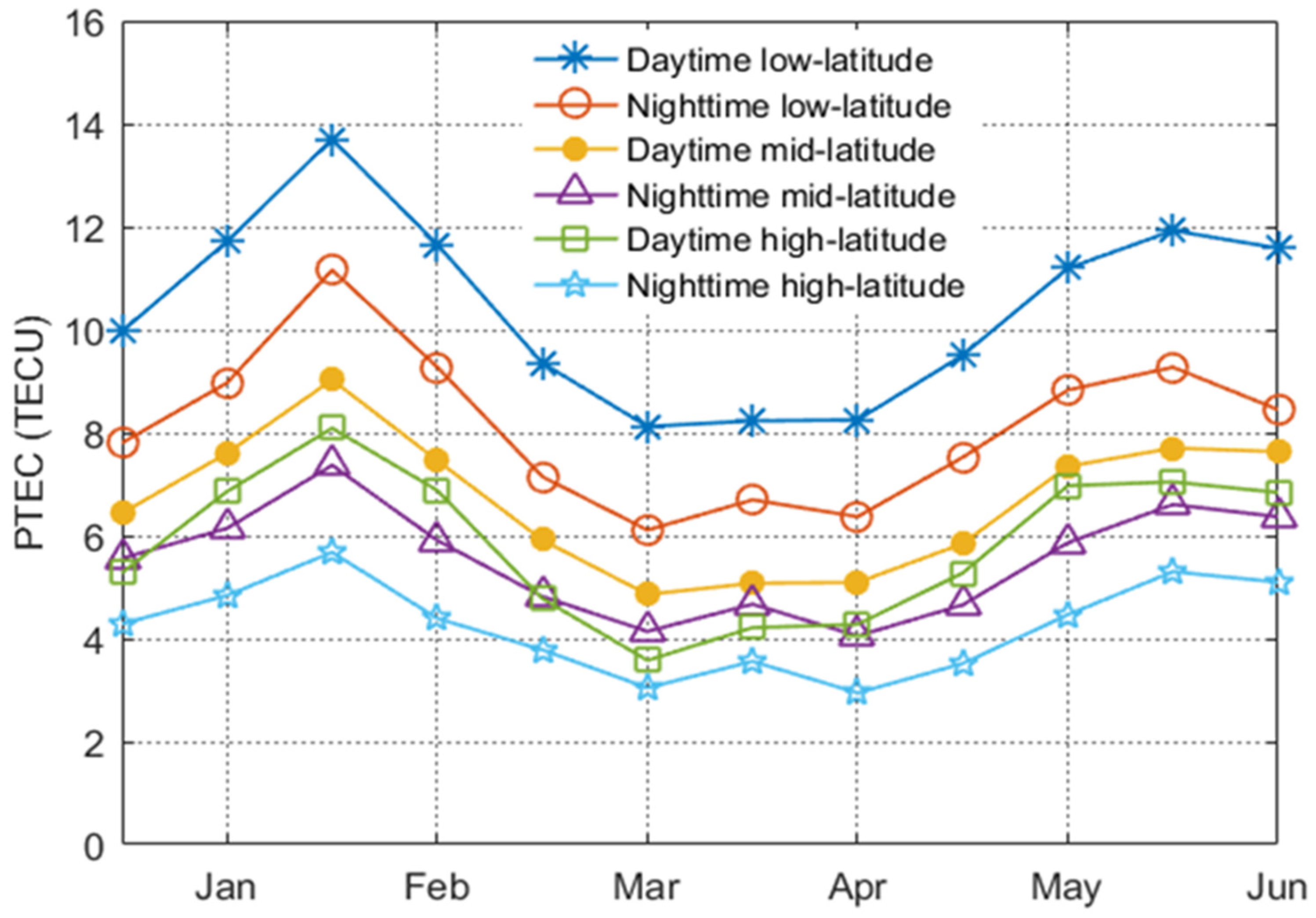
In the same way, we also analyzed the influence of magnetic local time and geomagnetic latitude on plasmaspheric TEC in 2014, during which year the solar activity was very active. An obvious feature is that the maximum values of plasmaspheric TEC in different regions all appeared in March, and the maximum reached 13.7 TECU in the daytime low-latitude region (
Figure 10). The variations of plasmaspheric TEC in different regions were relatively large, with a maximum variation range of about 5.6 TECU, and the relative variations were also greater than those in 2008. The same characteristics as 2008 were not repeated here. An obvious distinction is that values of plasmaspheric TEC in the daytime high-latitude region were higher than those in the nighttime mid-latitude region, except for January, June and July, which shows that the high-latitude region was more affected in intense periods of solar activity.
3.3. Correlation with Solar Activity
The plasmasphere is located above the Earth’s ionosphere with much lower particle density, but it is greatly affected by the solar radiation, which leads to the complex characteristics of plasmaspheric electron density variation. To study the relationship between plasmaspheric TEC and solar activity, we chose the F10.7 index as the reference indicator. There is a strong correlation between the 10.7 cm radio flux and the number or area of sunspots. At present, as one of the most important indices of solar activity, the F10.7 index has been widely used in space weather research and related studies of ionosphere and magnetosphere [
26].
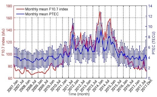
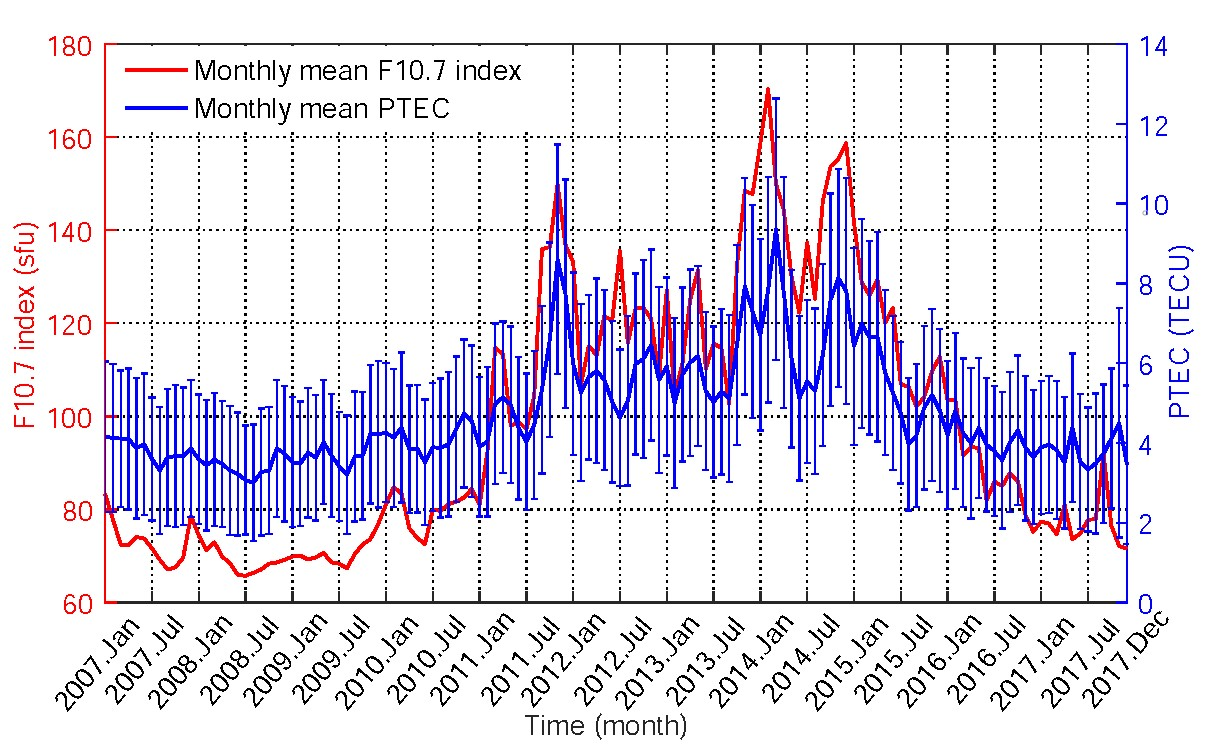
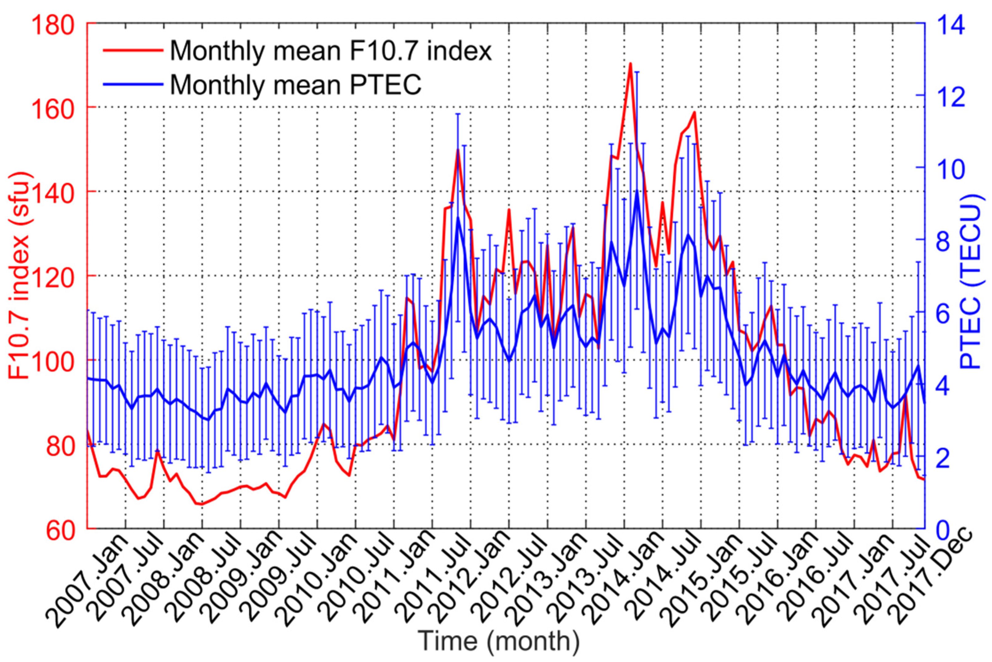
Figure 11 shows the monthly mean F10.7 indices and monthly mean PTEC from 2007 to 2017, where the red line represents the monthly mean F10.7 indices, corresponding to the left ordinate, and the blue line represents the plasmaspheric TEC, corresponding to the right ordinate. Before 2011, the monthly mean F10.7 indices were relatively small, and the variation was relatively gentle. During this period, the solar activity was relatively calm. After January 2011, the monthly mean F10.7 index rose sharply, and the variation was very intense, indicating that the solar activity was in an active period. Then, after 2015, the F10.7 index began to decline, and the solar activity decreased accordingly. The variation of monthly mean PTEC (the arithmetic average of PTEC at each grid point of the monthly plasmaspheric model) from 2007 to 2017 is shown in
Figure 11, and the standard deviation of each monthly mean PTEC is also calculated and shown with an error bar. Most of the standard deviations are less than 2.5 TECU, which indicates that the monthly mean PTEC is of significance. The values of monthly mean PTEC were also low before 2011, basically no more than 5 TECU, and the variation was relatively gentle. After 2011, the monthly mean PTEC also began to rise, and then began to decline after 2015, which was basically consistent with the variation of the monthly mean F10.7 indices.
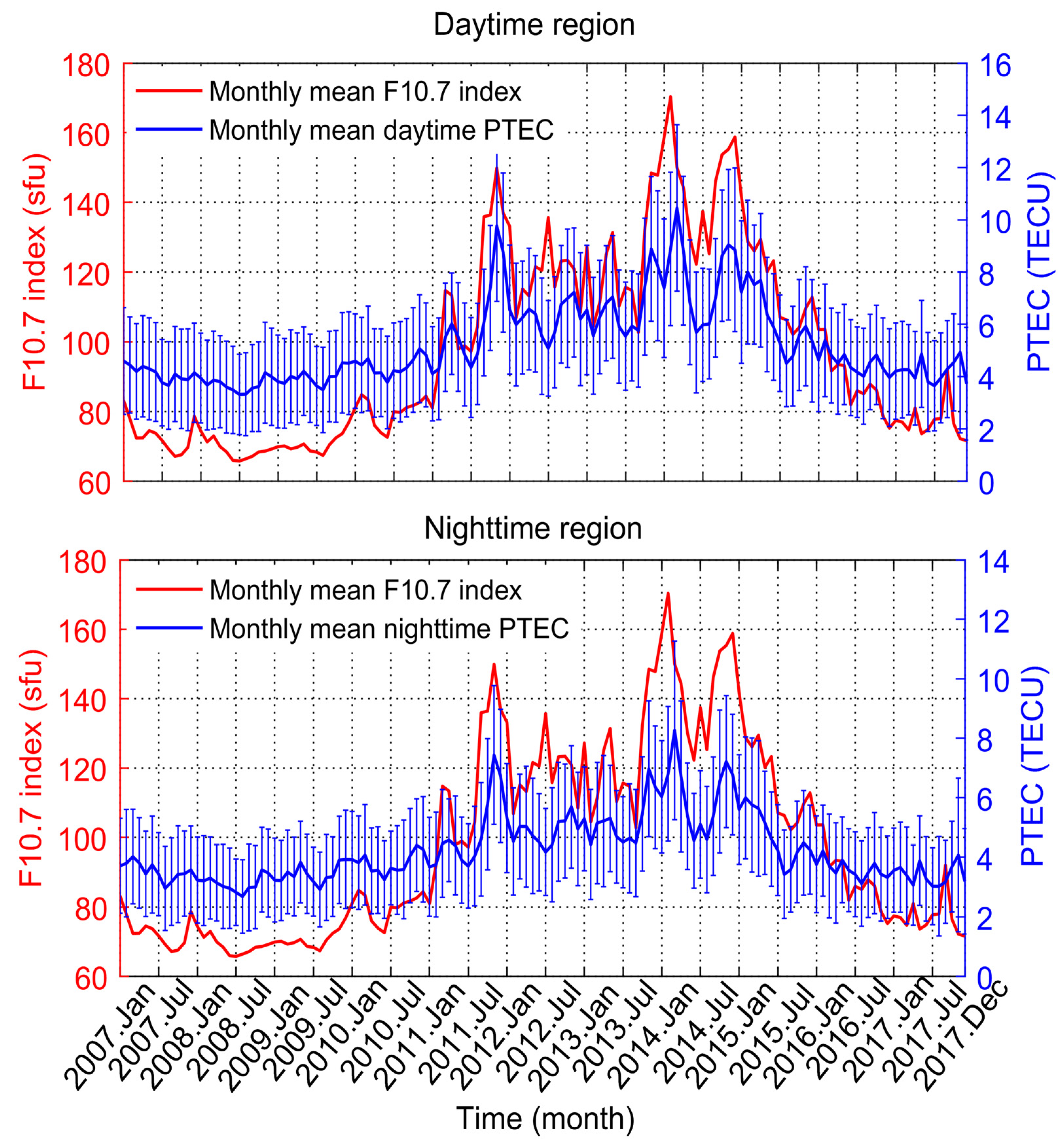
To determine the correlation between PTEC and solar activity in the daytime and nighttime, we divided the plasmaspheric TEC into the daytime region and nighttime region, and the division standard was the same as in the previous section. Similarly, the values of PTEC in the daytime and nighttime were averaged by month, respectively. The mean values and the standard deviations are shown in
Figure 12. The variations of PTEC in the daytime and nighttime are basically synchronous with differences less than 2 TECU, and both show consistency with the variation of the monthly mean F10.7 indices.
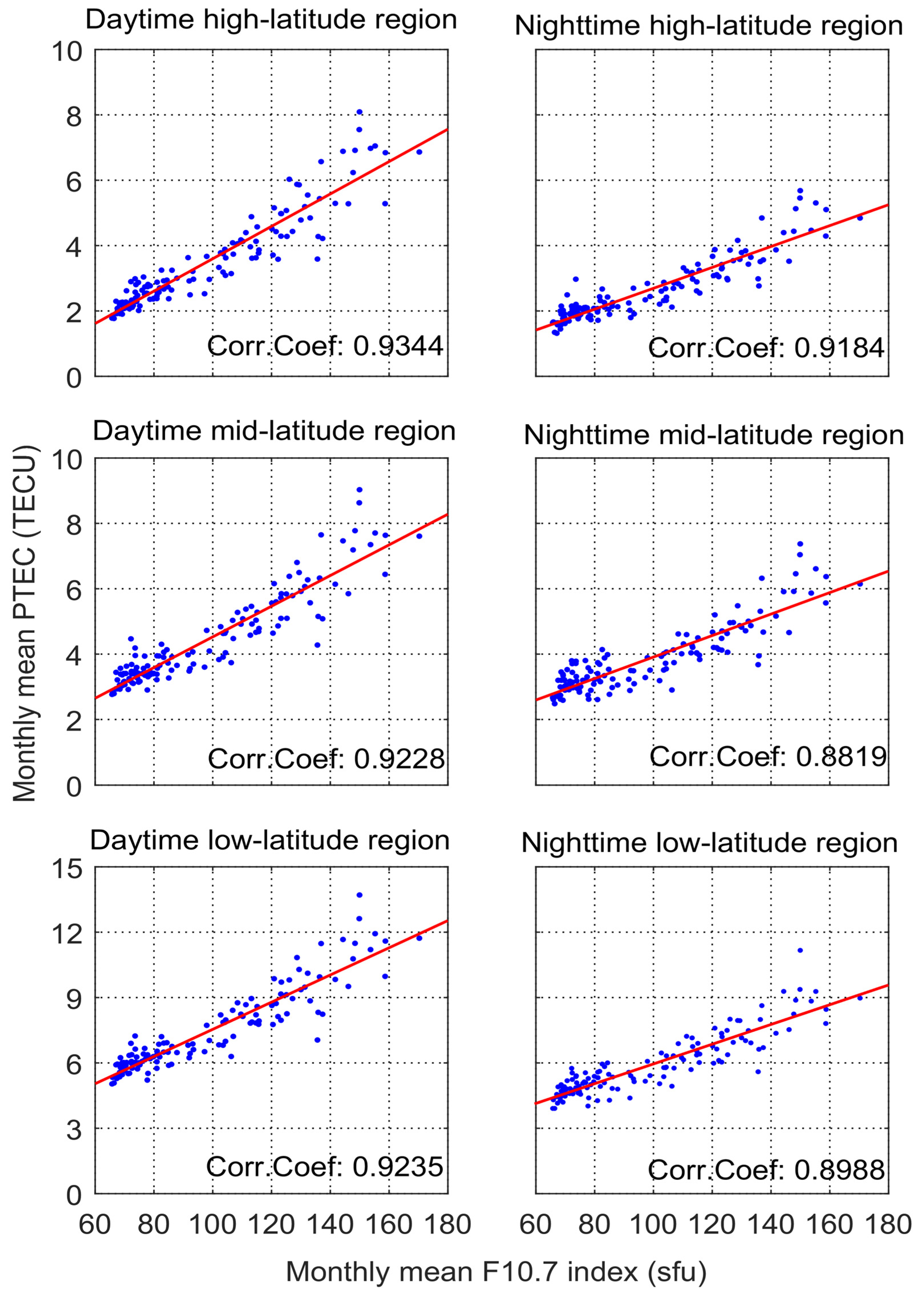
To further estimate the correlation between PTEC and the F10.7 index, we divided the monthly plasmaspheric TEC into latitudinal regions according to the geomagnetic latitude and the magnetic local time, and the criteria of division are the same as mentioned before. The monthly mean PTEC for each geomagnetic latitudinal region was calculated for daytime and nighttime. Then, they were counted with the corresponding monthly mean F10.7 indices in different subgraphs in
Figure 13. There are strong correlations between the monthly mean F10.7 indices and the monthly mean daytime and nighttime PTEC in each latitudinal region. In the same geomagnetic latitudinal region, the correlation between the monthly mean PTEC and the monthly mean F10.7 indices in the daytime is higher than that in the nighttime. This is because the plasmasphere in the daytime is directly exposed to the sun and can receive solar radiation and the energy directly, while in the nighttime, the plasmasphere is more affected by the ionosphere, which reduces the correlation with the solar activity. In the term of geomagnetic latitudinal region, the correlation in the geomagnetic high-latitude region is also the highest, while the geomagnetic middle-latitude region has the lowest correlation. However, among these correlation coefficients, the lowest one is still more than 0.88, indicating a very strong relationship between plasmaspheric TEC and the solar activity.
4. Conclusions
Using the topside GPS observations on COSMIC, the long-term plasmaspheric total electron content was obtained. By comparison with the GCPM, the plasmaspheric TEC from the topside observations of COSMIC was verified. Using the observation data in the solar minimum year 2008 and the solar maximum year 2014, PTEC was estimated at the monthly and seasonal scales, respectively, and its temporal-spatial distribution characteristics under different states of the solar activity were analyzed. The PTEC was mainly distributed in a belt region around the Earth within ±45° of the geomagnetic latitude. The plasmaspheric TEC in the daytime is higher than that in the nighttime, which reaches a peak between 14:00 and 17:00 in magnetic local time, while the minimum value of PTEC in the belt appears between 3:00 and 6:00 in magnetic local time before sunrise. For seasonal variations, the plasmaspheric TEC is the highest in the spring of the northern hemisphere and the lowest in the summer of the northern hemisphere, regardless of the state of solar activity. The variations of monthly mean PTEC in different regions were quite gentle during the solar minimum year 2008, while dramatical changes were found during the solar maximum year 2014. Furthermore, the long-term variations of the 11-year plasmaspheric TEC were analyzed with the F10.7 index as the reference indicator. The results showed a strong correlation between plasmaspheric TEC and solar activity.


 ,
, 


