
Semi-Supervised Multi-Temporal Deep Representation Fusion Network for Landslide Mapping from Aerial Orthophotos


1
Shenzhen Key Laboratory of IoT Intelligent Systems and Wireless Network Technology, The Chinese University of Hong Kong, Shenzhen 518172, China
2
CUHK(SZ)-CAS-NOVA Joint Laboratory, The Chinese University of Hong Kong, Shenzhen 518172, China
3
School of Mathematical Sciences, University of Science and Technology of China, Hefei 230026, China
4
Shenzhen Research Institute of Big Data, Shenzhen 518172, China
5
Shanghai CAS-NOVA Satellite Technology Company Limited, Shanghai 201210, China
*
Author to whom correspondence should be addressed.
Remote Sens. 2021, 13(4), 548; https://0-doi-org.brum.beds.ac.uk/10.3390/rs13040548
Submission received: 26 December 2020
/
Revised: 28 January 2021
/
Accepted: 28 January 2021
/
Published: 3 February 2021
(This article belongs to the Special Issue GeoAI: Integration of Artificial Intelligence, Machine Learning and Deep Learning with Remote Sensing)
Abstract
:Using remote sensing techniques to monitor landslides and their resultant land cover changes is fundamentally important for risk assessment and hazard prevention. Despite enormous efforts in developing intelligent landslide mapping (LM) approaches, LM remains challenging owing to high spectral heterogeneity of very-high-resolution (VHR) images and the daunting labeling efforts. To this end, a deep learning model based on semi-supervised multi-temporal deep representation fusion network, namely SMDRF-Net, is proposed for reliable and efficient LM. In comparison with previous methods, the SMDRF-Net possesses three distinct properties. (1) Unsupervised deep representation learning at the pixel- and object-level is performed by transfer learning using the Wasserstein generative adversarial network with gradient penalty to learn discriminative deep features and retain precise outlines of landslide objects in the high-level feature space. (2) Attention-based adaptive fusion of multi-temporal and multi-level deep representations is developed to exploit the spatio-temporal dependencies of deep representations and enhance the feature representation capability of the network. (3) The network is optimized using limited samples with pseudo-labels that are automatically generated based on a comprehensive uncertainty index. Experimental results from the analysis of VHR aerial orthophotos demonstrate the reliability and robustness of the proposed approach for LM in comparison with state-of-the-art methods.
1. Introduction
Landslides are among the most hazardous geological events that can cause widespread destructions, mass casualties, and substantial economic losses every year [1,2]. To better detect and monitor landslides, remote sensing (RS) techniques have attracted increasing attention in recent years [3,4,5]. Landslide mapping (LM) can be regarded as the quantification of land cover changes that are automatically derived from pre- and post-event RS imagery [6,7]. More specifically, LM records the attribute information of landslides, including the location, spatial extent, size, type, and date of occurrence [8,9]. This information is essential for quantitative hazard and risk assessment. Land cover change detection (CD) techniques based on multi-temporal RS datasets are usually selected to identify the differences between the pre- and post-event RS imagery and these changes are attributed to the landslide occurrence. Numerous CD methods have been developed for high-resolution RS imagery, including image difference, image transformation, post-classification comparison, and object-oriented analysis (OOA) [10,11]. In particular, the very-high-resolution (VHR) images can provide rich spectral information at the cost of enlarging the spectral heterogeneity within image objects, which incurs more speckle noises [11,12,13].
In the literature, existing LM methods using high-resolution images can be divided into pixel-based and object-based methods [14,15]. More specifically, pixel-based methods generally exploit the spatial information corresponding to each pixel or usually involve the multi-step pre-processing of images to reduce noise spots [16,17,18,19]. For instance, Cheng et al. [20] developed a semi-automatic method based on the band ratio to perform LM of SPOT images while Mondini et al. [21] developed an LM approach to directly compare and classify multi-temporal Quickbird images. Additionally, Li et al. [15] proposed a LM approach based on threshold segmentation and level set evolution and it has been proven to be effective in large-scale LM. The Markov random field (MRF) model, due to its superiority in combining spectral and spatial information, was introduced into LM to improve its accuracy [14,22].
In contrast, object-based methods take homogeneous image objects as processing units, aiming at classifying RS images into two classes, namely landslide and non-landslide, by image classification algorithms. For instance, Nichol and Wong [23] used unsupervised CD analysis based on multi-temporal segmentation at the object level and thresholding method to extract landslide-prone regions. In addition, Stumpf and Kerle [24] combined object-oriented analysis and random forest classification to perform LM. It reduced manual labor and improved feature selection and classification thresholds. Furthermore, Kurtz et al. [25] proposed a multi-resolution-based LM method to solve the spectral heterogeneity problems of landslide objects. Lv et al. [26] combined object-oriented multi-scale segmentation and the majority voting method to merge the spatial information of landslides and reduce heterogeneous pixels. Tavakkoli Piralilou et al. [27] combined object-oriented segmentation with the neural network and random forest for LM, and the optimal scale parameters were considered in the segmentation. Knevels et al. [28] investigated the potential of open-source geographic information system for object-based LM. The object-based methods were shown to provide LM results with fewer false positives and well-retained geometry compared with pixel-based methods [11]. However, these object-based methods still encounter challenges in many aspects such as feature selection, segmentation scale, and the training set size [29,30].
In recent years, deep learning has gained tremendous success in various remote-sensing applications due to its capability of unveiling latent representations from raw data [13,31]. Wang et al. [32] compared convolutional neural network (CNN) with four machine learning algorithms and the results demonstrated that CNN could achieve a better performance. However, CNN relied on its network structure, parameters settings, and training strategies, which limited its robustness [33]. In [34], deep CNNs with pyramid pooling were developed to merge multi-scale features for LM and Lv et al. [35] established a dual-path fully convolutional network model to extract landslides. One clear advantage of the CNN-based methods is that they can directly draw landslide maps without the generation of change magnitudes in an end-to-end manner.
Current deep learning-based LM methods mainly include three processes or modules, namely feature extraction, multi-temporal fusion, and network training [35]. Since deep learning-based image analysis extracts deep feature representations of the image patches for a given pixel, these representations are usually highly abstracted. As a result, it is generally difficult to retain precise outlines of the extracted objects during convolutions [36]. As LM is a multi-temporal feature fusion task, the extracted multi-temporal deep features are usually concatenated and fused by the convolutional functions to detect landslides [35]. However, spatio-temporal dependencies of deep features have been neglected. It has been proven that attention mechanism is capable of capturing channel and spatial dependencies of features [37]. With respect to the multi-temporal representation fusion, the non-linear relevance of features will be more sophisticated. In terms of network training, current deep learning approaches, together with feature extraction, require a large amount of labeled data, which can be an issue of concern in practice [38]. In order to reduce labeling efforts, semi-supervised deep learning has been widely used in the RS imagery analysis [39]. Pseudo-labels generated by the unsupervised clustering or classification algorithms are utilized to train the deep learning network [40]. Uncertainty analysis based on uncertainty indices such as Shannon entropy is an effective way to exploit pseudo-labels, in which data with low uncertainty have a high confidence of being correctly labeled [16,41].
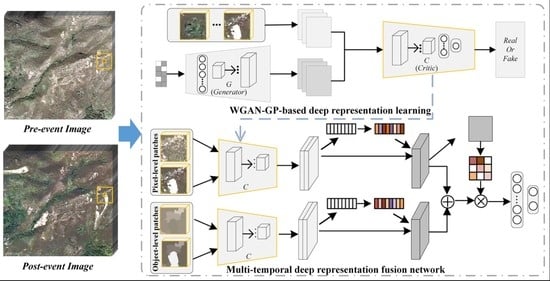
Motivated by the aforementioned challenges, this study proposes a semi-supervised multi-temporal deep representation fusion network (SMDRF-Net) for LM using the VHR aerial orthophotos. The proposed SMDRF-Net is developed by integrating multi-level deep representation learning (DRL) and multi-temporal deep representations fusion (DRF). The DRL is transferred from the Wasserstein generative adversarial network with gradient penalty (WGAN-GP) [42] through unsupervised adversarial training while the DRF is conducted by employing the attention mechanism to capture spatio-temporal interdependencies of multi-temporal and multi-level deep representations. The proposed LM framework is semi-supervised because the DRF network is optimized by the pseudo-labels that are automatically generated via unsupervised object-level CD and uncertainty analysis. To the best of our knowledge, it is the first time WGAN-GP-based DRL and attention-based DRF are applied for detecting landslides.
The contributions of this study include the following aspects:
- This study proposes a semi-supervised deep-learning-based LM framework for learning spatio-temporal relationships between pre- and post-event imagery and directly achieving LM results without manual annotations by automatically generating pseudo-labels based on a comprehensive uncertainty index.
- WGAN-GP is adopted to extract discriminative deep features through unsupervised adversarial training. It is then applied as the deep feature extractor in the SMDRF-Net through transfer learning to efficiently learn pixel- and object-level deep representations. This can improve the class separability between landslide and non-landslide patterns while retaining the precise outlines of landslide objects in the high-level feature space.
- The novel spatio-temporal DRF in the SMDRF-Net is developed to merge multi-temporal and multi-level deep representations using the channel and spatial attention; the former exploits the non-linear dependencies of multi-temporal deep feature maps whereas the latter characterizes the inter-spatial relationship of the combined representations. Integrating the two can further enhance the feature representation ability of network models.
2. Proposed Method
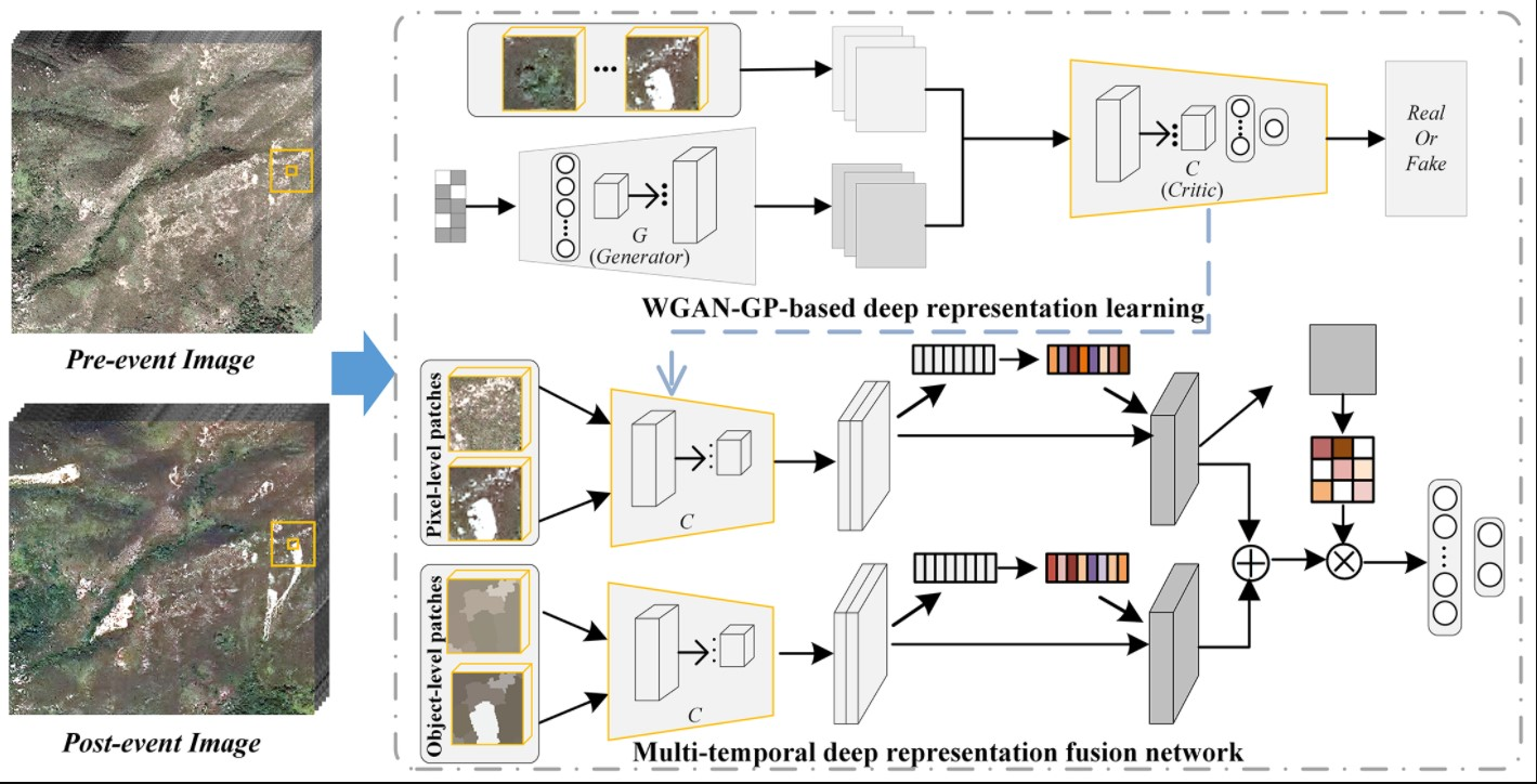
The general framework of the proposed LM approach is illustrated in Figure 1. First, the initial analysis is performed along with object-oriented CD. Multi-temporal co-segmentation and uncertainty analyses are conducted to exploit segmented image objects and generate the pseudo-labeling information of the landslides and non-landslide patterns. Next, the proposed SMDRF-Net is constructed by combining a multi-level DRL module and multi-temporal DRF module. Specifically, the WGAN-GP model with unlabeled image data is built through unsupervised adversarial training and the multi-level DRL module is developed by transfer learning from the WGAN-GP model to generate pixel- and object-level deep representations of the pre- and post-event imagery. Furthermore, the multi-temporal DRF module is developed based on the novel channel-spatial attention mechanisms to model the spatio-temporal dependencies of deep representations. The network is then optimized using limited samples with pseudo-labels. These samples have a high confidence of being correctly labeled and they can provide considerable supervised information containing landslide and non-landslide patterns for the network training. Finally, pixel-wise LM results are derived from the predictions of the trained network.
2.1. Initial CD and Analysis
The pre- and post-event images, I1 and I2 each having B bands, are stacked and co-segmented via object-oriented image analysis to create homogeneous image objects with spatially consistent boundaries in multi-temporal images. The fractal net evolution approach (FNEA) is conducted on the stacked images to generate segmented objects. More specifically, FNEA splits an image into homogeneous regions and the optimal segment parameters are determined with the aid of the estimation of scale parameter (ESP) tool as reported in [43]. Based on unsupervised CD methods, the object-level change intensity map can be obtained using the following equation:
where S(i) is the change intensity of the ith pixel belonging to the pth object and Qp denotes the pixel number in the region denoted by Rp that the pth object covers.
The fast fuzzy C-means (FCM) clustering algorithm is incorporated into the framework to effectively cluster areas into two categories, namely, landslide and non-landslide, by minimizing the following objective function via an iterative process [44]:
where P is the total number of objects and L = 2 LM categories with l = 1 and l = 2 representing the landslide and non-landslide categories, respectively. Furthermore, is the cluster center of the lth category while upl is the fuzzy membership of the pth object associated with the lth cluster derived from the fast FCM.
Subsequently, the fuzzy uncertainty of each pixel is characterized by a comprehensive uncertainty index (CUI):
The CUI is developed by combining the Shannon entropy [16], and square error [45], to measure the uncertainty of each object label. It is normalized to fall within (0,1). Pixels with low uncertainty and their corresponding labels can be chosen as pseudo-labeling samples in ascending order of uncertainty values. Then, the pseudo-training set with the sample size of M can be obtained.
2.2. The Proposed SMDRF-Net
The proposed deep learning network contains two modules, namely the multi-level DRL module and multi-temporal DRF module. The DRL network is constructed with transfer learning from the adversarial training of the WGAN-GP model to extract pixel- and object-level deep features of multi-temporal imagery. The DRF network is built based on the channel-spatial attention mechanism to fuse the multi-temporal and multi-level deep representations for the classification task. The resulting network then performs the pixel-wise classification decision for LM.
2.2.1. Unsupervised DRL with WGAN-GP
For the unlabeled post-event imagery I2 with B bands, we use the image patch containing the ith pixel and its spatial neighborhood as the input data to learn the abstract representations, where represents the window size of its neighborhood. The generative adversarial network (GAN) model consists of a generator and a discriminator. It is adopted to learn reusable deep representations from unlabeled data in an unsupervised manner using the image patches and some noises that obey a fixed distribution [46].
Considering noise sources, the generator can generate synthetic data and the discriminator discriminates between the real data and synthetic data. These two models compete against each other during the training process in the form of a zero-sum game to improve their functionalities. GANs have proven useful for unsupervised and semi-supervised learning as a form of generative model [47]. Parts of the discriminator networks can then be used as feature extractors for supervised tasks such as classification and CD [48]. However, training a GAN model is challenging due to possible training instability or convergence failure.
The WGAN has made significant progress in the training of GANs by adopting the metric of Wasserstein distance for measuring the distance between the discriminator’s and the generator’s distribution [49]. The WGAN discriminator is more actually called a ‘critic’ instead of a ‘discriminator’ because it is used to narrow the difference between the deep features of the real data and the generated samples instead of discriminating between the real and synthetic data. As reported by Arjovsky et al. [49], the critic in WGAN must satisfy the Lipschitz-continuity, i.e., the gradient of each point in the defined domain does not exceed a certain constant. WGAN uses weight clipping to force Lipschitz restrictions in the critic; however, it sometimes produces low-quality samples and does not converge on certain settings.
Compared with WGAN, WGAN-GP [42] adds a soft constraint on the critic’s gradient regularization term to enforce Lipschitz constraints instead of weight clipping. As a result, this method converges more quickly and can produce higher-quality samples. The gradient penalty term in WGAN-GP can keep the gradient stable during the backward propagation process and solve the problem of slow convergence that exists in the original WGAN [42].
The generator and critic loss functions in WGAN-GP are as follows:
where and are the loss functions of the generator G and the critic C, respectively. The variable is the expectation operator, is the gradient penalty coefficient, denotes the real data distribution, and represents the generator’s distribution over data defined by , in which the input z to the generator is sampled from some simple noise distribution . is sampled uniformly by linear interpolation between the data distribution and the distribution of generated samples , i.e., where is a random number and .
In this study, the generator consists of a fully connected (FC) layer, a series of convolutional (Conv) layers, upsampling (UP) layers, batch normalization (BN) layers, and rectified linear unit (ReLU) layers. The critic is composed of multiple fractional-strided Conv layers followed by BN layers and leaky version of ReLU (LeakyReLU) layers, together with FC layers. The two networks compete against each other during the training process and their parameters are updated alternately.
2.2.2. Multi-Level DRL Module Based on Transfer Learning
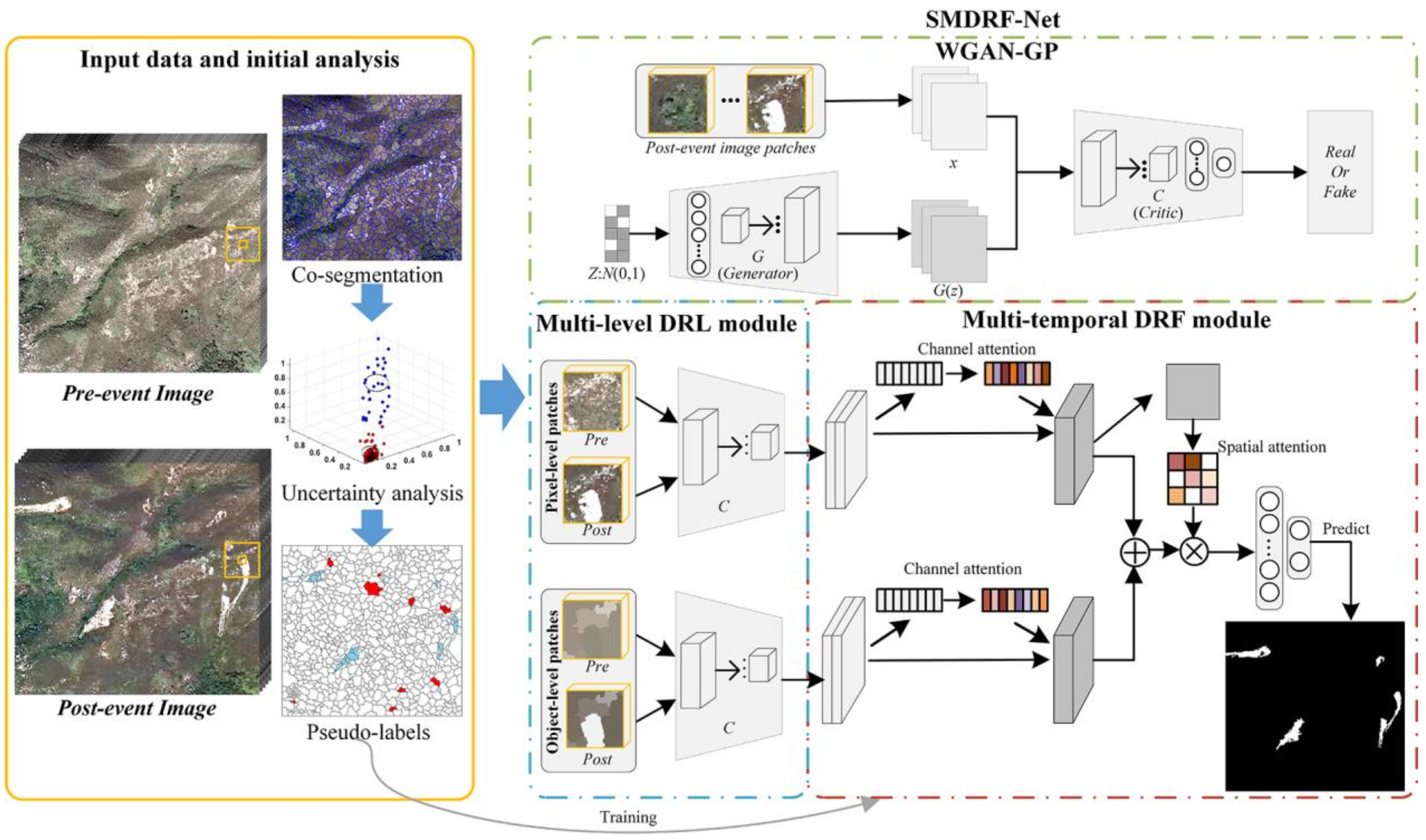
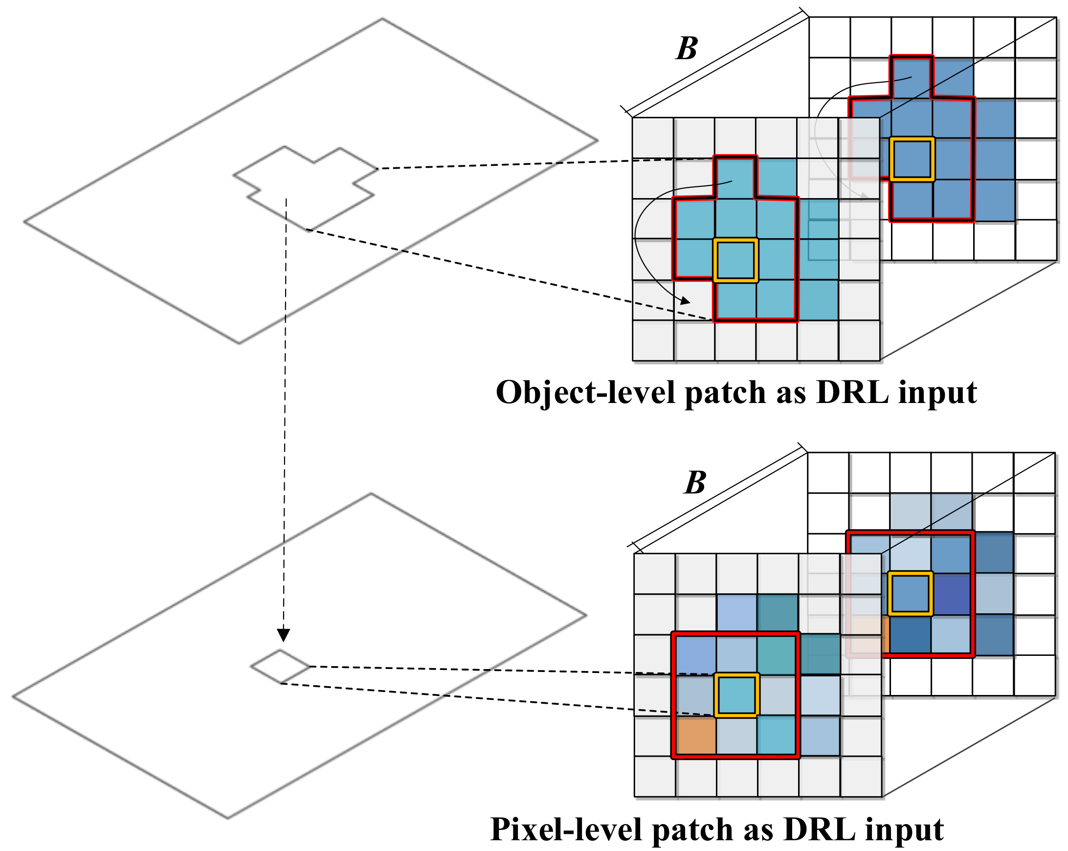
The critic of WGAN-GP after the adversarial training can extract discriminant features from unlabeled data. More specifically, the pixel- and object-level deep features can be generated from the convolutional streams of the critic with transfer learning, as illustrated in Figure 1. We use the image patch with all bands centering around the given pixel as the pixel-level input of the network while exploiting the object-level input by using the object spectral value with the same size as the pixel-level input, as shown in Figure 2. These input feature patches can be expressed as follows:
where represents the image patch of the ith pixel at time t while is the object-level feature of the ith pixel. Furthermore, is the spectral mean value of the object covering the ith pixel at the bth band.
With respect to the adversarial training of the WGAN-GP model, the deep representations can be extracted by cascading convolutional streams of the critic:
where stands for the deep representations of image patch
and denotes the convolutional streams with the depth of n.
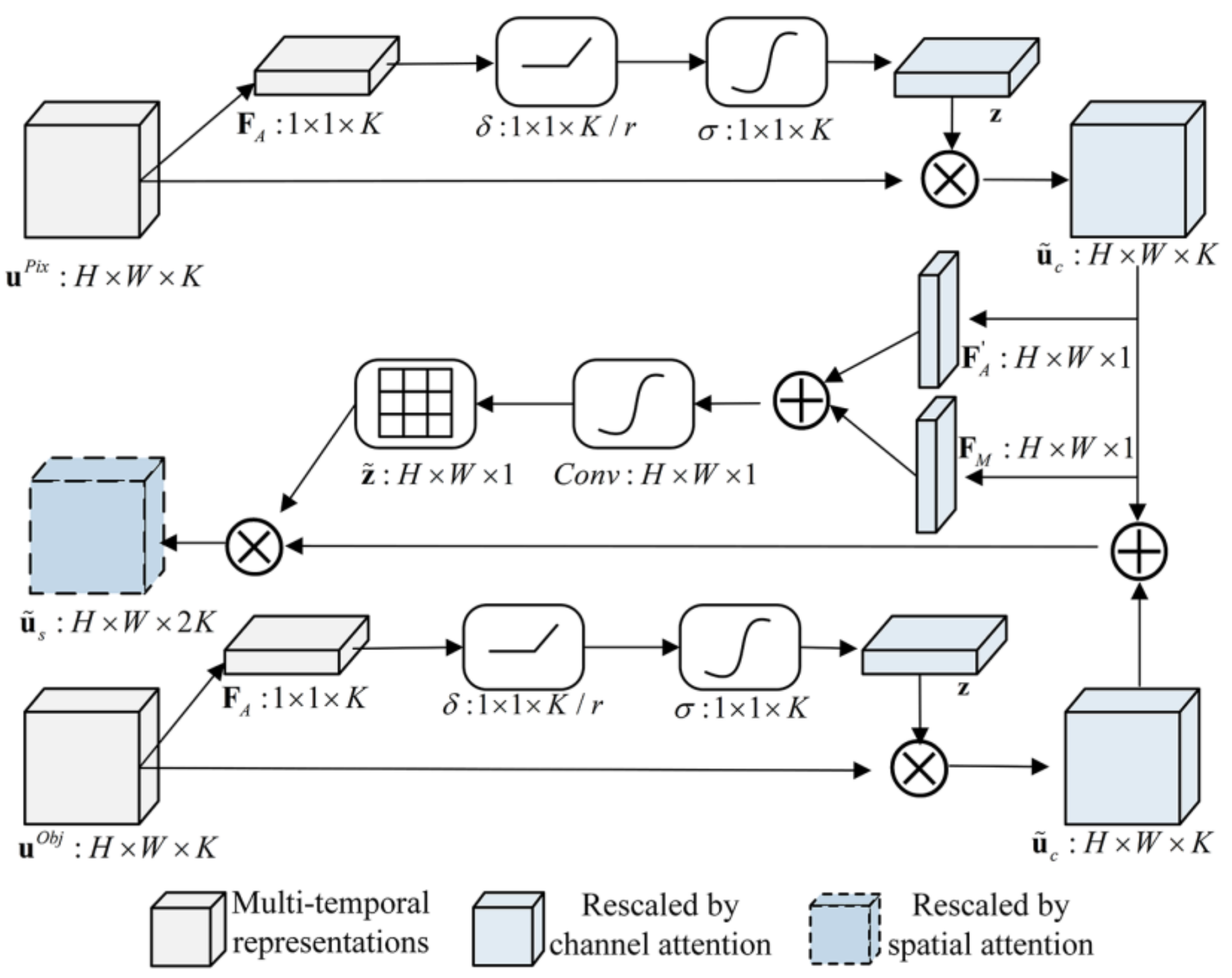
2.2.3. Attention-Based Multi-Temporal DRF Module
To make full use of the extracted deep representations, we employ the attention mechanism to capture the spatio-temporal dependencies of multi-temporal and multi-level deep representations [50]. The channel attention is used to exploit the inter-channel relationship of multi-temporal features and the spatial attention focusses on identifying the informative part along the spatial axis considering the importance of each pixel location [51]. The details of the proposed DRF are displayed in Figure 3.
The pixel- and object-level deep representations, i.e., and obtained by the DRL module can be expressed as:
where the symbol denotes the operation of concatenating the feature vectors. Accordingly, the channel-level attention coefficients for the feature maps can be calculated based on a gating function with a sigmoid activation :
where and represent the trainable parameters with K and r being the dimension of deep features and the dimensionality-reduction ratio, respectively. Furthermore, refers to the ReLU function. The function performs feature compression along the spatial axis and turns each 2-D feature channel into a real number using global average pooling to obtain a global receptive field. The gating function can learn a non-mutually-exclusive relationship between multiple channels [52] to enhance target-relevant features while filtering out irrelevant features of the combined multi-temporal representations. Thus, it becomes possible to transform the feature map by rescaling as follows:
where represents the rescaled deep representations by the channel attention and denotes the element-wise multiplication function between deep representations and attention coefficients . Furthermore, the importance of each pixel location is recalibrated to characterize the beneficial information across the spatial dimension and improve the feature representation capability. Two branches, i.e., and , are further merged based on the spatial attention mechanism.
Two pooling operations, i.e., average-pooling and max-pooling , are applied to rescaled pixel-level deep representations to gather channel information and generate an efficient feature descriptor along the spatial axis. After this is completed, the spatial attention map can be obtained as follows:
where denotes a convolution operation. The object-level deep representations can be rescaled by the element-wise multiplication between deep representations and the spatial attention map . As a result, the importance of each pixel location can be iteratively recalibrated during the network training so that it characterizes the beneficial information across the spatial dimension. Then, the rescaled deep representations by the spatial attention can be obtained as follows:
where represents the rescaled deep representations by the spatial attention which can be further followed by a FC layer and a Softmax layer at the end of the network to conduct the classification task.
3. Experiments and Analyses
3.1. Dataset Descriptions
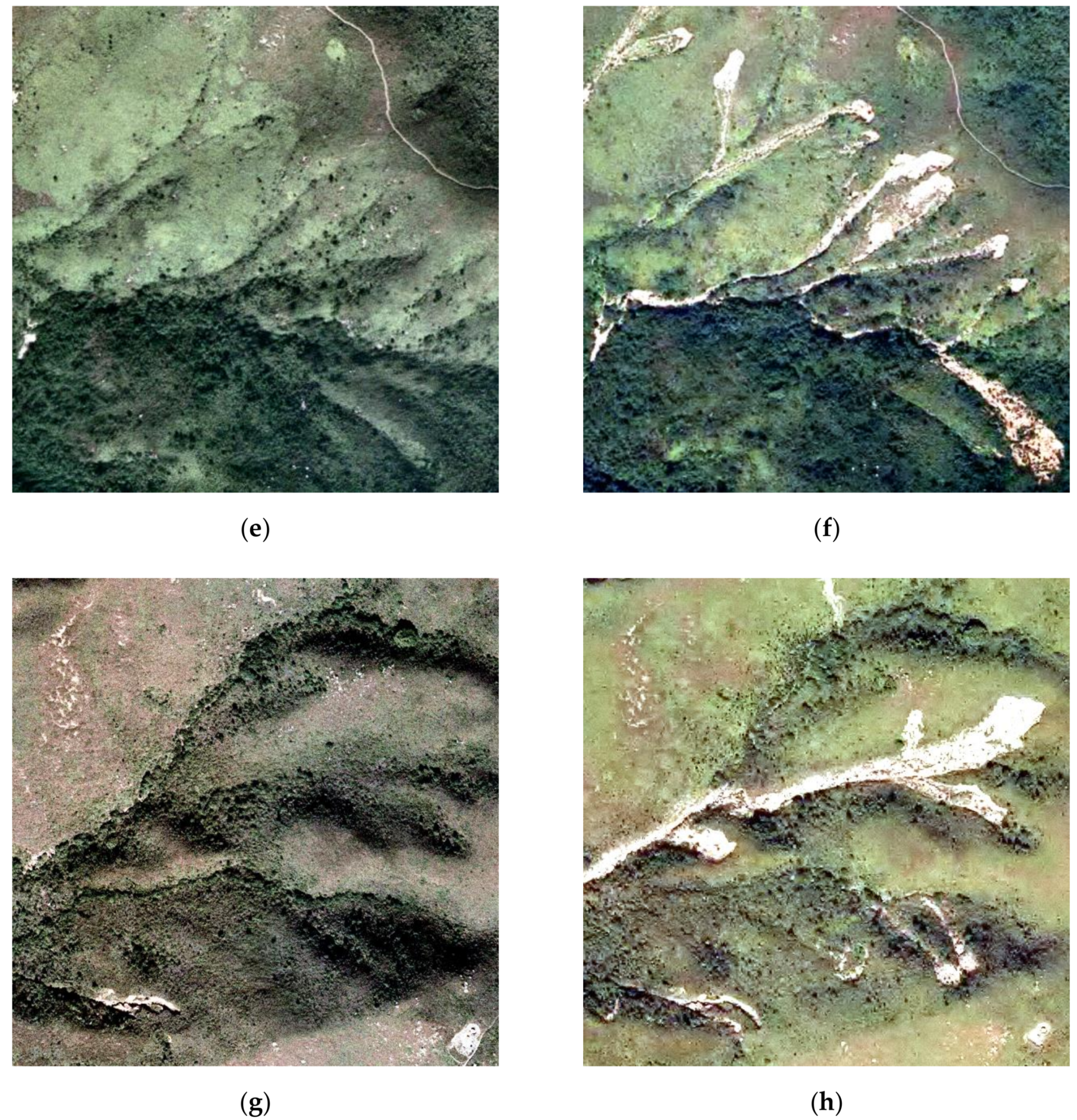
Four datasets, namely, Datasets A, B, C, and D, were used as the experimental data, as shown in Figure 4 and Table 1. The datasets were acquired using Zeiss RMK top-level aerial survey camera systems, and each contained pre- and post-event aerial orthophotos of the Lantau Island, Hong Kong, China, as shown in Figure 5. A great number of landslides and debris flows occurred because of the heavy rainfall and we chose four of the most damaged areas as the study sites. The bi-temporal images in the four datasets had three bands (i.e., RGB) with the same spatial resolution of 0.5 m. Details of the experimental datasets in this study are shown in Table 1 and the study area locations are illustrated in Figure 4. The test datasets contain landslides that occurred in varied land cover conditions with topographic heterogeneity, as shown in Table 1. For example, Dataset C is covered with dense grasslands and sparse woodlands, while numerous volcanic rocks exist in Dataset B, which have similar spectral features to landslides and pose challenges to LM. What is more, these landslides are different in shape and size, as shown in Figure 5. Pre-processing, including co-registration and radiation correction, through ENVI software was performed on the multi-temporal images to reduce the influence of positioning and radiometric errors on the results; this allowed us to directly compare the multi-temporal images. Ground-truth maps were produced via manual interpretation using the editor tool of ESRI ArcGIS 10.7 [53].
3.2. Experimental Setting
3.2.1. General Information
The proposed approach was compared with the following two unsupervised LM algorithms: the change-detection-based MRF (CDMRF) model [22] and the object-based majority voting (OMV) method [26]. Furthermore, we benchmarked our proposed approach against two semi-supervised deep learning methods, i.e., the superpixel-based difference representation learning (SDRL) algorithm [54] and the semi-supervised GAN-based (SGAN) CD method [55]. To verify the effectiveness of the proposed approach, the following five indicators were used as the quantitative evaluation criteria:
- Completeness (CP): , where is the number of correctly detected landslide pixels and indicates the number of real landslide pixels in the ground truth map;
- Correctness (CR): , where is the number of all detected landslide pixels;
- Quality (QA): , where is the number of misdetected landslide pixels;
- Kappa coefficient (KC): , where and are the proportion of agreement and chance agreement with respect to the confusion matrix, respectively;
- Overall Accuracy (OA): , where is the number of incorrectly detected landslide pixels in the LM map and is the total number of pixels in the ground truth map.
3.2.2. Network Structures
In the proposed framework, the input image size of the network was 9×9 pixels with three channels (i.e., 9×9×3). The critic in the WGAN-GP was composed of two Conv layers with depths of 32 and 64 and the kernel size was 3×3 pixels with stride 2 in each layer. Each Conv layer was followed by the BN layer and the LeakyReLU layer parameterised by 0.2. The outputs of the last LeakyReLU layer were flattened to 1-D before they were put into the FC layers and the activation function was deprecated in the output layer. With respect to the generator, the input noises were fed into the FC layer and reshaped to a three-dimensional tensor followed by two UP layers and three Conv layers. We adopted 4×4 Conv layers with depths of 128, 64, and 3 and strides of 1 followed by BN layers and ReLU layers except the last Conv layer where the Tanh was applied.
The Conv layers together with BN layers and LeakyReLU layers in the critic were transferred from WGAN-GP to the multi-level DRL module. After that, the generated deep representations were fused based on the channel-spatial attention, and then fed into a FC layer with 200 neurons and a Softmax layer for the classification task.
3.2.3. Network Training
In the proposed framework, the parameters of Scale, Shape, and Compactness in the FANE algorithm were set to 30, 0.7, and 0.8, respectively, with the aid of the ESP tool. Subsequently, the generated object features were incorporated into the SMDRF-Net. The size M of pseudo-labeled samples was set to 4000, and the landslide and non-landslide sample sets were assigned the same size, i.e., M/2.
We set the following parameters for the WGAN-GP training: the gradient penalty coefficient ; the batch size ; the number of critic iterations per generator iteration ; and the Adam hyperparameters , , and . The SMDRF-Net did not need to learn new deep features of imagery because the deep features extraction process was completed by the multi-level DRL module. Thus, training the SMDRF-Net actually implied training the multi-temporal DRF module. The parameters of the DRF network were updated using the Adam optimizer. We fixed all the parameters of Adam by setting , , and . All network weights were initialized with a Glorot uniform distribution. In addition, the dimensionality-reduction ratio r in the DRF network was set to 8. Finally, the samples and pseudo-labels obtained by the initial CD and uncertainty analysis were fed into the network to train the proposed deep learning network. The cross-entropy loss function was adopted to measure the difference between the predicted value and the actual label as follows:
We used a smaller minibatch size of 32 and trained the network for 50 epochs. The training was implemented on a TensorFlow 2.0.0 (GPU) framework on a workstation with a graphics card of NVIDIA GeForce RTX 2080 Ti.
3.3. Results and Analysis
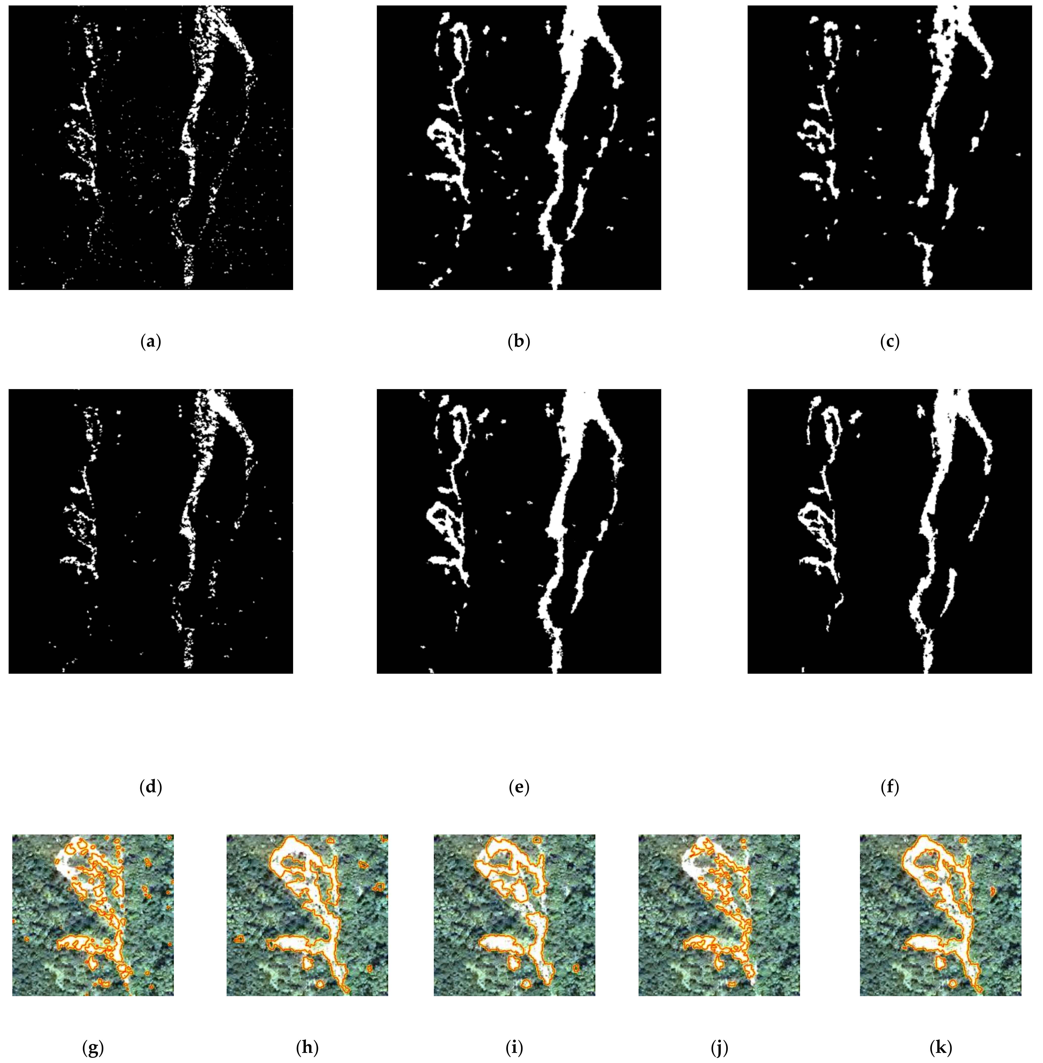
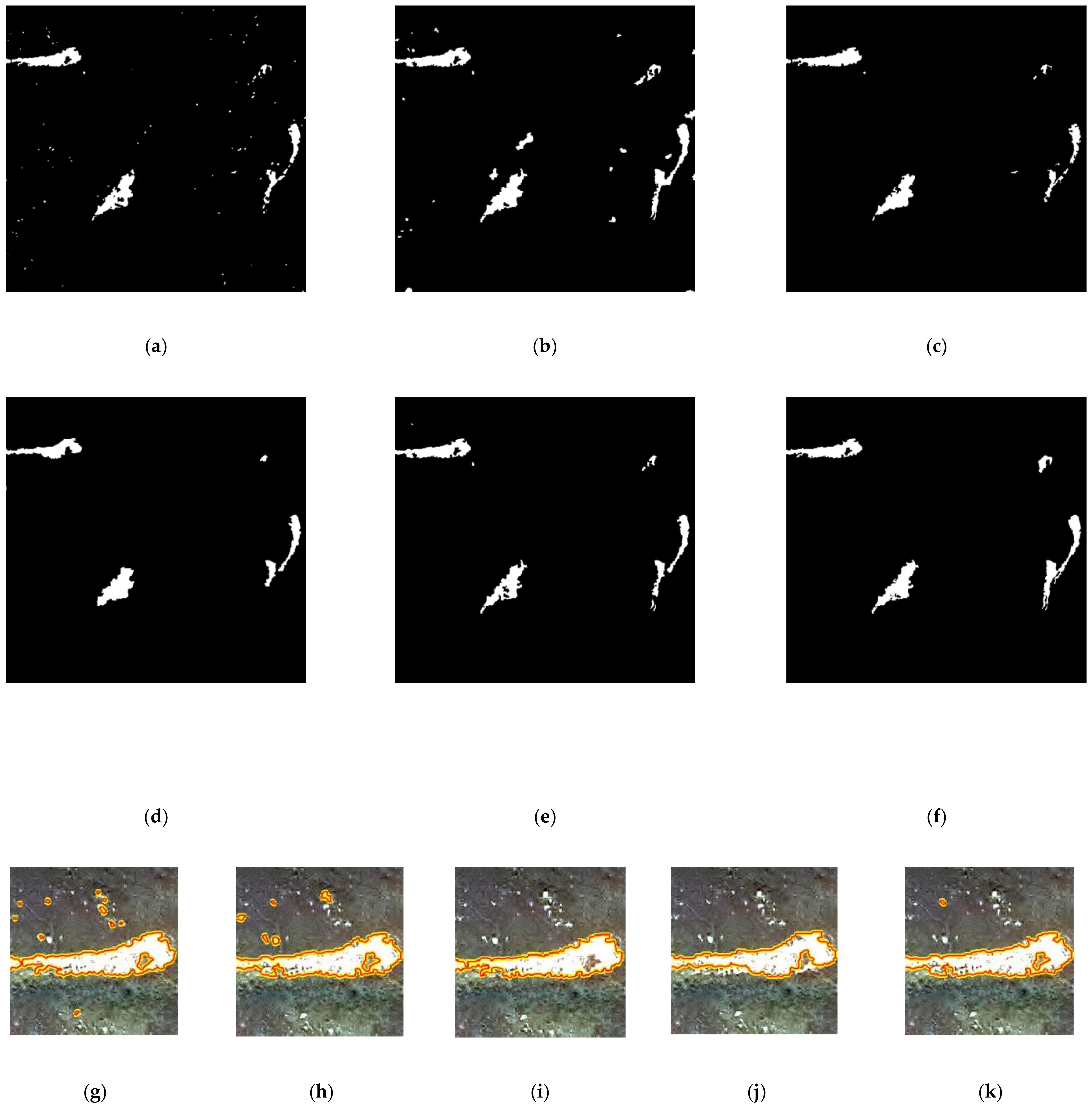
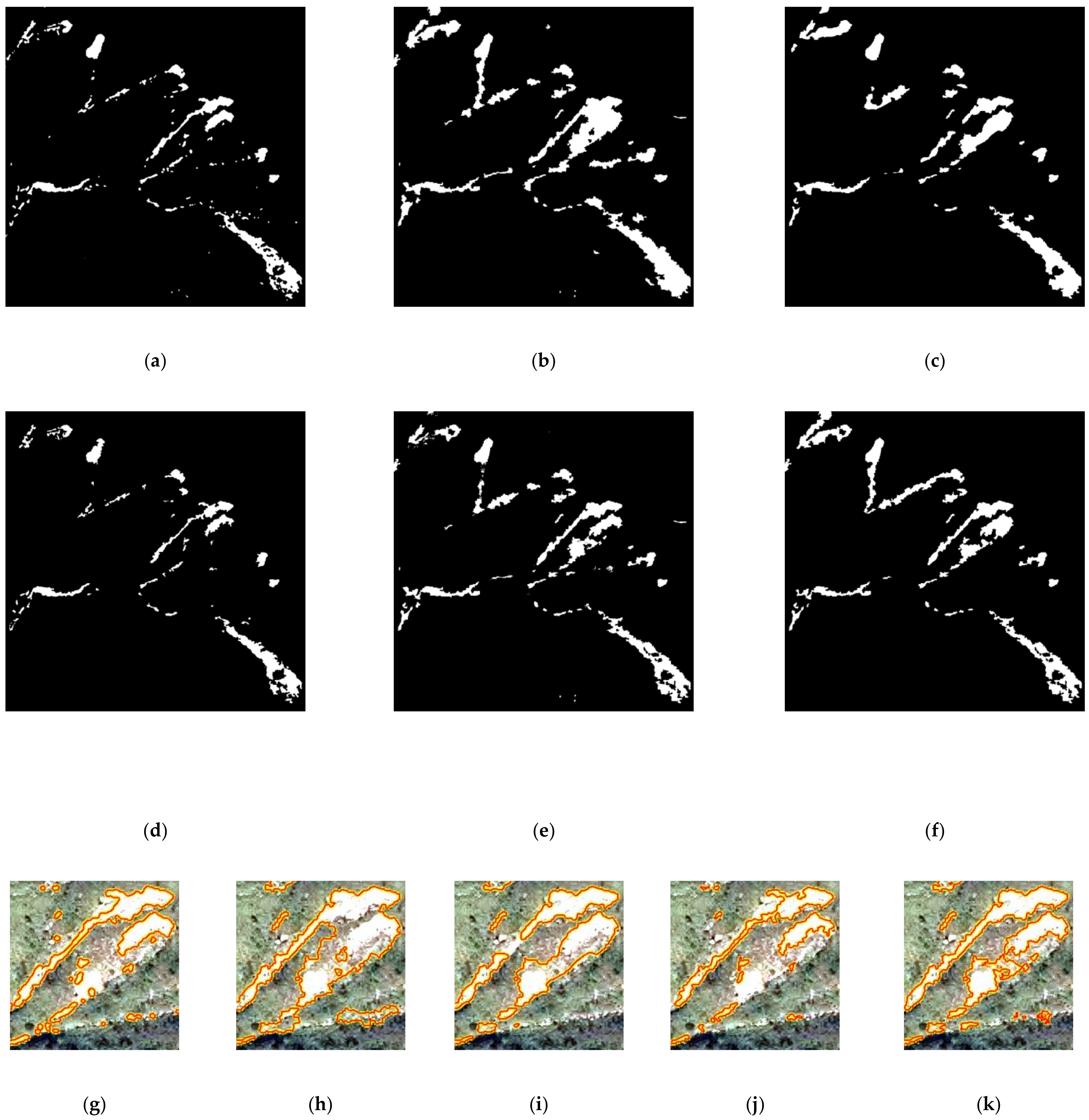
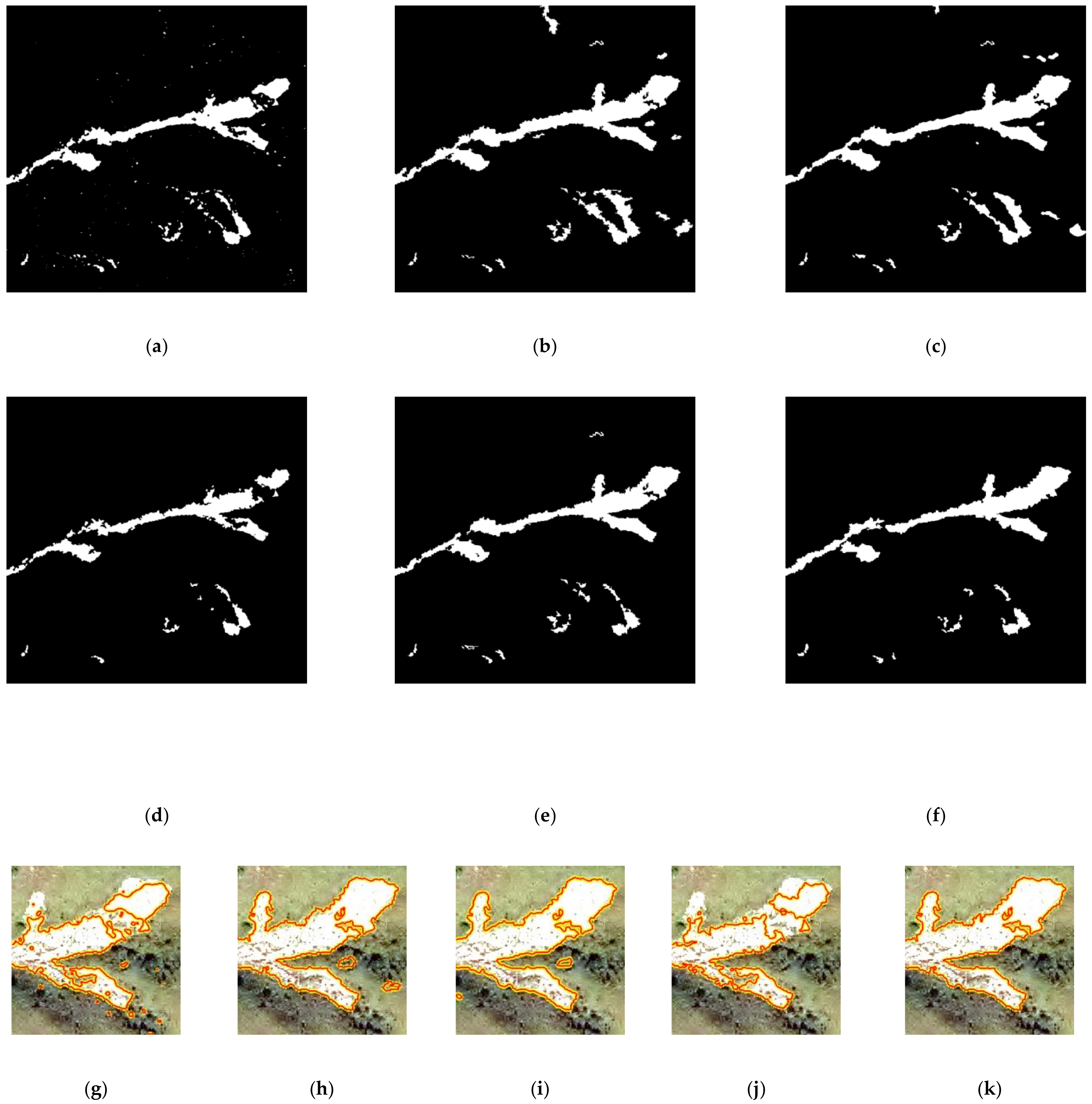
The LM results for the test datasets are shown in Figure 6, Figure 7, Figure 8 and Figure 9. The quantitative evaluation of each algorithm is shown in Table 2. It is evident that CDMRF suffers from significant noise and generates some omissions, resulting in lower CP scores and higher QA values. On the other hand, OMV yields some object-level false alarms and loses some details of landslide objects, as shown in Figure 6b,h. As shown in Table 2, OMV obtains higher CP scores, but some misclassifications lead to a decreased CR. With respect to SGAN, although false alarms can be reduced to some extent, as illustrated in Figure 7d,j, its use still results in the misdetection of some landslide regions because discriminators obtained through adversarial training are used to extract deep features. The corresponding LM maps have lower QA values, as shown in Table 2. In addition, some accurately labeled samples are required for fine-tuning SGAN [55]. Compared to CDMRF, OMV, and SGAN, the SDRL which uses local and high-level representations from deep neural networks offers effective detection of homogenous landslide regions, but it still suffers from losses of detailed information in the boundaries, as shown in Figure 6c and Figure 9c. In contrast, the proposed approach can achieve a higher level of performance for all the evaluation indicators. Specifically, the highest CP, CR, QA, KC, and OA values are 0.92, 0.92, 0.83, 0.90, and 99.59%, respectively, as shown in Table 2. In addition, it can retain detailed landslide regions while significantly reducing noise, as shown in Figure 6k, Figure 7k, Figure 8k and Figure 9k.
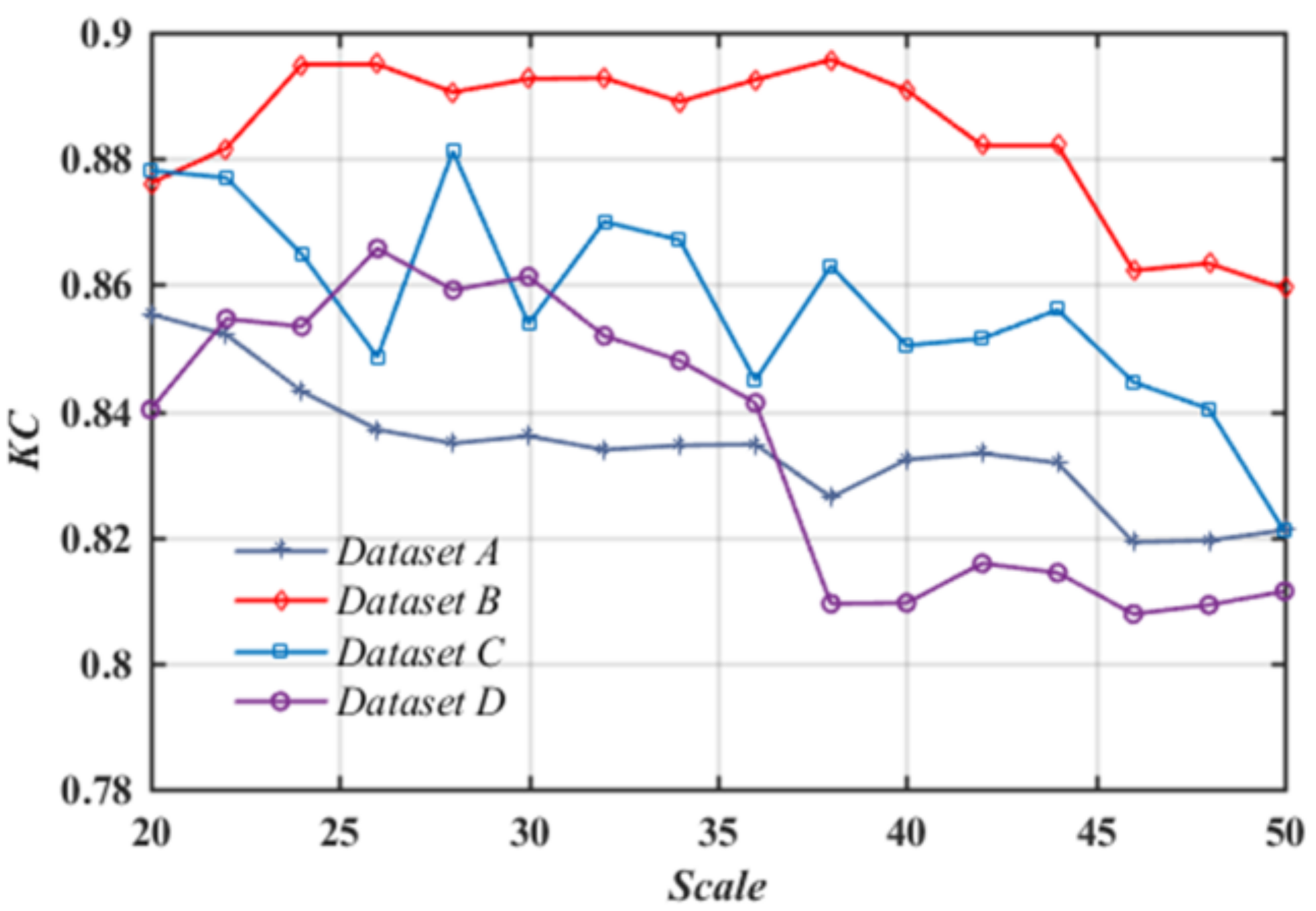
The Scale parameter is the key control for the object-oriented analysis of RS images. It is correlated with the average size, amount, and boundaries of image objects [30]. To test the influence of the segmentation scale on the proposed approach, we set different Scale parameters of FANE ranging from 20 to 60 with a step size of 2 to generate multi-scale segmentation maps and obtain the corresponding LM results, as shown in Figure 10. It can be found that the KC remains at a high level with lower scales. When the scale exceeds a certain value, the segmented objects cannot remain accurate boundaries of objects, and the accuracy performance begins to degrade.
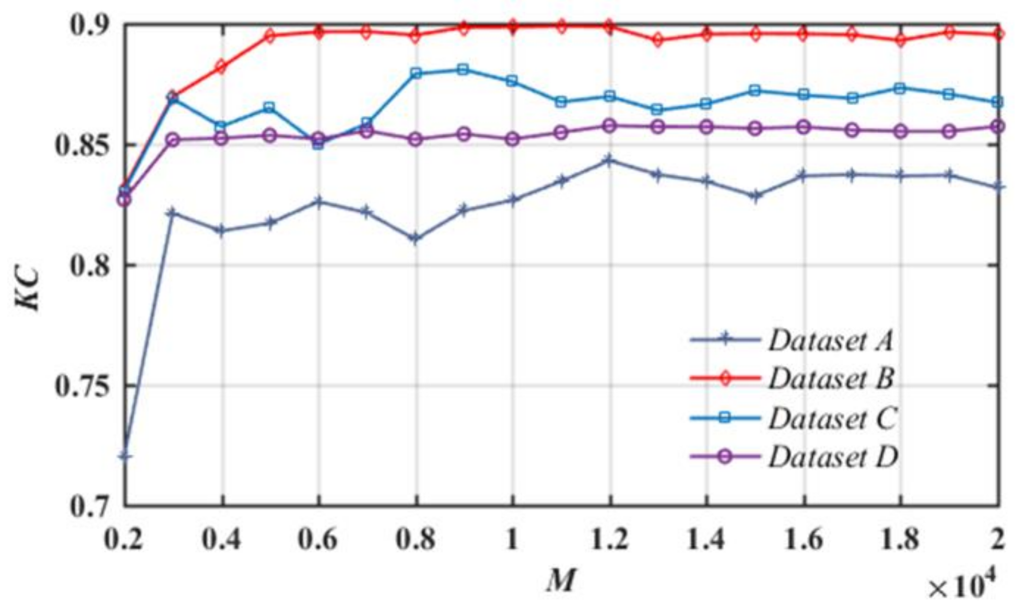
Different LM maps achieved by different sample size values, i.e., M, ranging from 2000 to 20,000 with a step size of 1000 were used to analyze the effects of different sample sizes on LM results. The relationships between the KC and different M values in the proposed model are displayed in Figure 11. A small M value may result in poor prediction performance of the model because of the poor representativeness of the samples. As M increases, the overall accuracy also increases and becomes stable at a higher level.
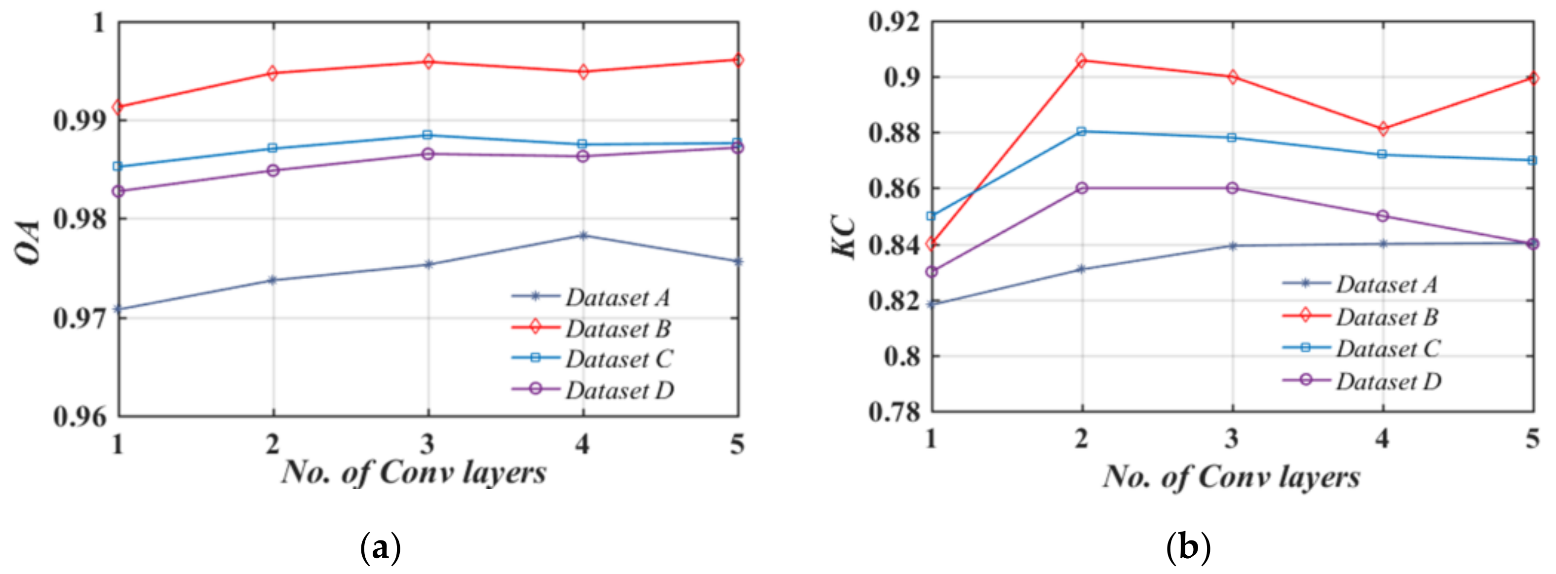
The convolutional layers in the critic of the WGAN-GP model are used for deep feature extraction and the quality of the learnt representations is significantly affected by the depth of the DRL network and the level of abstraction. As shown in Figure 12, the network with 1 Conv layer results in a lower accuracy because the critic is not well trained during the training of the WGAN-GP. With the increasing of the number of the Conv layers, the critic networks can learn more abstract deep representations with increased complexity and training time.
4. Discussion
The experimental results on four multi-temporal VHR datasets indicate that the proposed SMDRF-Net is superior to the test LM methods through the quantitative and qualitative analysis. Specifically, the SMDRF-Net obtains the highest accuracy among all methods in the experiment, as shown in Table 2. In comparison with other deep learning-based LM methods, the SMDRF-Net has some distinct properties:
The SMDRF-Net performs unsupervised DRL based on WGAN-GP to exploit discriminative deep representations and the critic of WGAN-GP with multiple Conv blocks can be used as the unsupervised feature exactor, as shown in Figure 12.
Deep learning can transform original images into abstract high-level representations and as the network becomes deeper, it is difficult to retain accurate outlines of targets. In order to solve this problem, the proposed approach incorporates the object-level spectral features to exploit deep representations of objects. As a result, it can retain accurate boundaries of landslide objects while reducing noises, as displayed in the zoomed areas of Figure 6, Figure 7, Figure 8 and Figure 9. In addition, we test the effect of the Scale parameters on LM accuracies by generating multi-scale segmentation maps and the results have shown that LM accuracies can remain stable within a certain interval of Scale values, as illustrated in Figure 10. It is indicated that the proposed approach is robust to object segmentation scales.
In other LM models, the multi-temporal deep features are usually concatenated and fused by the convolutional functions. With respect to the proposed approach, the spatio-temporal attention is incorporated into the DRF module, which can enhance landslide-relevant features and recalibrate the importance of each pixel location during the network training. Therefore, it enables the SMDRF-Net to capture the spatio-temporal relationships of multi-temporal deep features more accurately. From the evaluations of CR, CP, and QA in Table 2, it can be found that the generated LM maps can restrict false alarms and omissions while maintaining complete landslide areas.
As the proposed approach adopts unsupervised DRL, only the DRF module requires training samples. We use a sample-selection strategy based on unsupervised object-level CD and uncertainty analysis to choose reliable pseudo-labels for the DRF training. As a result, the SMDRF-Net can get well-fitted with a relatively small number of pseudo-labels, as shown in Figure 11, contrary to other models that rely on enormous manually labeled samples for network training.
The primary limitation of the proposed approach is that the SMDRF-Net relies on object-oriented segmentations and object spectral features as the prior information for the network training, and this could increase the algorithm complexity. As the object-level deep representations are exploited in the network, the dimension of features is increased, and hence more computational resources are necessary.
5. Conclusions
In this study, a novel LM approach has been developed based on the semi-supervised multi-temporal deep representation fusion network (SMDRF-Net). The SMDRF-Net is capable of learning discriminative representations from pre- and post-event images and generating LM results in an end-to-end training fashion. After training the WGAN-GP with unlabeled image data, a critic network is applied as a deep feature extractor on the multi-temporal imagery to obtain discriminative deep representations. By integrating the pixel- and object-level DRL, the class separability can be improved and outlines of landslide objects can be well-retained in the high-level feature space. Furthermore, the DRF module based on the attention mechanism is employed to learn the spatio-temporal relationships of deep representations by exploiting the non-linear interdependencies of multi-temporal deep feature maps and the inter-spatial relationships of the combined representations. Limited samples with pseudo-labels generated automatically are used for optimizing the network to produce the pixel-wise LM result. Our experimental results on VHR aerial orthophotos have shown that the proposed approach performs competitively with other state-of-the-art LM approaches. Notably, the proposed approach can significantly improve the reliability of the LM results with minimum manual annotation efforts. Furthermore, the LM results produced by this approach are robust against the object segmentation scale and the training sample size. Future improvements will focus on LM using multi-temporal data from different sensors based on semi-supervised deep representation fusion and transfer learning.
Author Contributions
Conceptualization, X.Z.; Formal analysis, M.L.; Investigation, M.-O.P.; Methodology, X.Z. and M.-O.P.; Resources, M.L.; Validation, X.Z., M.-O.P. and M.L.; Writing–original draft, X.Z.; Writing – review & editing, X.Z. and M.-O.P. All authors have read and agreed to the published version of the manuscript.
Funding
This research was funded by National Natural Science Foundation of China, grant number 41801323, China Postdoctoral Science Foundation, grant number 2020M682038 and Shenzhen Science and Technology Innovation Committee, grant numbers ZDSYS20170725140921348 and JCYJ20190813170803617.
Institutional Review Board Statement
Not applicable.
Informed Consent Statement
Not applicable.
Data Availability Statement
Data sharing not applicable.
Acknowledgments
The authors would like to thank Wenzhong Shi and Zhiyong Lv for providing the wonderful datasets and also the editors and reviewers whose comments have significantly improved this paper.
Conflicts of Interest
The authors declare no conflict of interest.
References
- Park, N.-W.; Chi, K. Quantitative assessment of landslide susceptibility using high-resolution remote sensing data and a generalized additive model. Int. J. Remote Sens. 2008, 29, 247–264. [Google Scholar] [CrossRef]
- Yang, X.; Chen, L. Using multi-temporal remote sensor imagery to detect earthquake-triggered landslides. Int. J. Appl. Earth Obs. 2010, 12, 487–495. [Google Scholar] [CrossRef]
- Ciampalini, A.; Raspini, F.; Bianchini, S.; Frodella, W.; Bardi, F.; Lagomarsino, D.; Di Traglia, F.; Moretti, S.; Proietti, C.; Pagliara, P.; et al. Remote sensing as tool for development of landslide databases: The case of the Messina Province (Italy) geodatabase. Geomorphol. 2015, 249, 103–118. [Google Scholar] [CrossRef]
- Hervás, J.; Barredo, I.J.; Rosin, P.L.; Pasuto, A.; Mantovani, F.; Silvano, S. Monitoring landslides from optical remotely sensed imagery: The case history of Tessina landslide, Italy. Geomorphol. 2003, 54, 63–75. [Google Scholar] [CrossRef]
- Liu, P.; Li, Z.; Hoey, T.; Kincal, C.; Zhang, J.; Zeng, Q.; Muller, J.-P. Using advanced InSAR time series techniques to monitor landslide movements in Badong of the Three Gorges region, China. Int. J. Appl. Earth Obs. Geoinformation 2013, 21, 253–264. [Google Scholar] [CrossRef]
- Lu, P.; Stumpf, A.; Kerle, N.; Casagli, N. Object-Oriented Change Detection for Landslide Rapid Mapping. IEEE Geosci. Remote Sens. Lett. 2011, 8, 701–705. [Google Scholar] [CrossRef]
- Metternicht, G.; Hurni, L.; Gogu, R. Remote sensing of landslides: An analysis of the potential contribution to geo-spatial systems for hazard assessment in mountainous environments. Remote Sens. Environ. 2005, 98, 284–303. [Google Scholar] [CrossRef]
- Zhong, C.; Liu, Y.; Gao, P.; Chen, W.; Li, H.; Hou, Y.; Nuremanguli, T.; Ma, H. Landslide mapping with remote sensing: Challenges and opportunities. Int. J. Remote Sens. 2020, 41, 1555–1581. [Google Scholar] [CrossRef]
- Guzzetti, F.; Mondini, A.C.; Cardinali, M.; Fiorucci, F.; Santangelo, M.; Chang, K.-T. Landslide inventory maps: New tools for an old problem. Earth-Science Rev. 2012, 112, 42–66. [Google Scholar] [CrossRef] [Green Version]
- Lv, Z.; Liu, T.; Wan, Y.; Benediktsson, J.A.; Zhang, X. Post-Processing Approach for Refining Raw Land Cover Change Detection of Very High-Resolution Remote Sensing Images. Remote Sens. 2018, 10, 472. [Google Scholar] [CrossRef] [Green Version]
- Keyport, R.N.; Oommen, T.; Martha, T.R.; Sajinkumar, K.; Gierke, J.S. A comparative analysis of pixel- and object-based detection of landslides from very high-resolution images. Int. J. Appl. Earth Obs. Geoinformation 2018, 64, 1–11. [Google Scholar] [CrossRef]
- Lv, Z.; Liu, T.; Benediktsson, J.A. Object-Oriented Key Point Vector Distance for Binary Land Cover Change Detection Using VHR Remote Sensing Images. IEEE Trans. Geosci. Remote Sens. 2020, 58, 6524–6533. [Google Scholar] [CrossRef]
- Zhang, X.; Shi, W.; Lv, Z.; Peng, F. Land Cover Change Detection from High-Resolution Remote Sensing Imagery Using Multitemporal Deep Feature Collaborative Learning and a Semi-supervised Chan–Vese Model. Remote Sens. 2019, 11, 2787. [Google Scholar] [CrossRef] [Green Version]
- Lu, P.; Qin, Y.; Li, Z.; Mondini, A.C.; Casagli, N. Landslide mapping from multi-sensor data through improved change detection-based Markov random field. Remote Sens. Environ. 2019, 231, 111235. [Google Scholar] [CrossRef]
- Li, Z.; Shi, W.; Myint, S.W.; Lu, P.; Wang, Q. Semi-automated landslide inventory mapping from bitemporal aerial photographs using change detection and level set method. Remote Sens. Environ. 2016, 175, 215–230. [Google Scholar] [CrossRef]
- Zhang, X.; Shi, W.; Liang, P.; Hao, M. Level set evolution with local uncertainty constraints for unsupervised change detection. Remote Sens. Lett. 2017, 8, 811–820. [Google Scholar] [CrossRef]
- Zhang, X.; Shi, W.; Hao, M.; Shao, P.; Lyu, X. Level set incorporated with an improved MRF model for unsupervised change detection for satellite images. Eur. J. Remote Sens. 2017, 50, 202–210. [Google Scholar] [CrossRef] [Green Version]
- Bazi, Y.; Melgani, F.; Al-Sharari, H.D. Unsupervised Change Detection in Multispectral Remotely Sensed Imagery With Level Set Methods. IEEE Trans. Geosci. Remote Sens. 2010, 48, 3178–3187. [Google Scholar] [CrossRef]
- Bazi, Y.; Bruzzone, L.; Melgani, F. An unsupervised approach based on the generalized Gaussian model to automatic change detection in multitemporal SAR images. IEEE Trans. Geosci. Remote Sens. 2005, 43, 874–887. [Google Scholar] [CrossRef] [Green Version]
- Cheng, K.-S.; Wei, C.; Chang, S. Locating landslides using multi-temporal satellite images. Adv. Space Res. 2004, 33, 296–301. [Google Scholar] [CrossRef]
- Mondini, A.C.; Guzzetti, F.; Reichenbach, P.; Rossi, M.; Cardinali, M.; Ardizzone, F. Semi-automatic recognition and mapping of rainfall induced shallow landslides using optical satellite images. Remote Sens. Environ. 2011, 115, 1743–1757. [Google Scholar] [CrossRef]
- Li, Z.; Shi, W.; Lu, P.; Yan, L.; Wang, Q.; Miao, Z. Landslide mapping from aerial photographs using change detection-based Markov random field. Remote Sens. Environ. 2016, 187, 76–90. [Google Scholar] [CrossRef] [Green Version]
- Nichol, J.; Wong, M.S. Satellite remote sensing for detailed landslide inventories using change detection and image fusion. Int. J. Remote Sens. 2005, 26, 1913–1926. [Google Scholar] [CrossRef]
- Stumpf, A.; Kerle, N. Object-oriented mapping of landslides using Random Forests. Remote Sens. Environ. 2011, 115, 2564–2577. [Google Scholar] [CrossRef]
- Kurtz, C.; Stumpf, A.; Malet, J.-P.; Gançarski, P.; Puissant, A.; Passat, N. Hierarchical extraction of landslides from multiresolution remotely sensed optical images. ISPRS J. Photogramm. Remote Sens. 2014, 87, 122–136. [Google Scholar] [CrossRef] [Green Version]
- Lv, Z.; Shi, W.; Zhang, X.; Benediktsson, J.A. Landslide Inventory Mapping From Bitemporal High-Resolution Remote Sensing Images Using Change Detection and Multiscale Segmentation. IEEE J. Sel. Top. Appl. Earth Obs. Remote Sens. 2018, 11, 1520–1532. [Google Scholar] [CrossRef]
- Piralilou, S.T.; Shahabi, H.; Jarihani, B.; Ghorbanzadeh, O.; Blaschke, T.; Gholamnia, K.; Meena, S.R.; Aryal, J. Landslide Detection Using Multi-Scale Image Segmentation and Different Machine Learning Models in the Higher Himalayas. Remote Sens. 2019, 11, 2575. [Google Scholar] [CrossRef] [Green Version]
- Knevels, R.; Petschko, H.; Leopold, P.; Brenning, A. Geographic Object-Based Image Analysis for Automated Landslide Detection Using Open Source GIS Software. ISPRS Int. J. Geo-Information 2019, 8, 551. [Google Scholar] [CrossRef] [Green Version]
- Hussain, M.; Chen, D.; Cheng, A.; Wei, H.; Stanley, D. Change detection from remotely sensed images: From pixel-based to object-based approaches. ISPRS J. Photogramm. Remote Sens. 2013, 80, 91–106. [Google Scholar] [CrossRef]
- Drăguţ, L.; Csillik, O.; Eisank, C.; Tiede, D. Automated parameterisation for multi-scale image segmentation on multiple layers. ISPRS J. Photogramm. Remote Sens. 2014, 88, 119–127. [Google Scholar] [CrossRef] [Green Version]
- Ma, L.; Liu, Y.; Zhang, X.; Ye, Y.; Yin, G.; Johnson, B.A. Deep learning in remote sensing applications: A meta-analysis and review. ISPRS J. Photogramm. Remote Sens. 2019, 152, 166–177. [Google Scholar] [CrossRef]
- Wang, H.; Zhang, L.; Yin, K.; Luo, H.; Li, J. Landslide identification using machine learning. Geosci. Front. 2021, 12, 351–364. [Google Scholar] [CrossRef]
- Ghorbanzadeh, O.; Blaschke, T.; Gholamnia, K.; Meena, S.R.; Tiede, D.; Aryal, J. Evaluation of Different Machine Learning Methods and Deep-Learning Convolutional Neural Networks for Landslide Detection. Remote Sens. 2019, 11, 196. [Google Scholar] [CrossRef] [Green Version]
- Lei, T.; Zhang, Y.; Lv, Z.; Li, S.; Liu, S.; Nandi, A.K. Landslide Inventory Mapping From Bitemporal Images Using Deep Convolutional Neural Networks. IEEE Geosci. Remote Sens. Lett. 2019, 16, 982–986. [Google Scholar] [CrossRef]
- Lv, Z.; Liu, T.; Kong, X.; Shi, C.; Benediktsson, J.A. Landslide Inventory Mapping with Bitemporal Aerial Remote Sensing Images Based on the Dual-path Full Convolutional Network. IEEE J. Selected Topics Appl. Earth Observ. Remote Sens. 2020, 58, 4575–4584. [Google Scholar] [CrossRef]
- Zhao, W.; Du, S.; Emery, W.J. Object-Based Convolutional Neural Network for High-Resolution Imagery Classification. IEEE J. Sel. Top. Appl. Earth Obs. Remote Sens. 2017, 10, 3386–3396. [Google Scholar] [CrossRef]
- Fu, J.; Liu, J.; Tian, H.; Li, Y.; Bao, Y.; Fang, Z.; Lu, H. Dual Attention Network for Scene Segmentation. In Proceedings of the 2019 IEEE/CVF Conference on Computer Vision and Pattern Recognition (CVPR), Long Beach, CA, USA, 16–20 June 2019; IEEE: IEEE, 2019; pp. 3141–3149. [Google Scholar]
- Pan, B.; Shi, Z.; Xu, X. MugNet: Deep learning for hyperspectral image classification using limited samples. ISPRS J. Photogrammetry Remote Sens. 2018, 145, 108–119. [Google Scholar] [CrossRef]
- Wu, H.; Prasad, S. Semi-Supervised Deep Learning Using Pseudo Labels for Hyperspectral Image Classification. IEEE Trans. Image Process. 2018, 27, 1259–1270. [Google Scholar] [CrossRef]
- Yang, M.; Jiao, L.; Liu, F.; Hou, B.; Yang, S. Transferred Deep Learning-Based Change Detection in Remote Sensing Images. IEEE Trans. Geosci. Remote Sens. 2019, 57, 6960–6973. [Google Scholar] [CrossRef]
- Zhang, X.; Shi, W.; Lv, Z. Uncertainty Assessment in Multitemporal Land Use/Cover Mapping with Classification System Semantic Heterogeneity. Remote Sens. 2019, 11, 2509. [Google Scholar] [CrossRef] [Green Version]
- Gulrajani, I.; Ahmed, F.; Arjovsky, M.; Dumoulin, V.; Courville, A.C. Improved training of wasserstein gans. Adv. Neur. Inf. Proc. Syst. 2017, 30, 5767–5777. [Google Scholar]
- Drăgut, L.; Tiede, D.; Levick, S.R. ESP: A tool to estimate scale parameter for multiresolution image segmentation of remotely sensed data. Int. J. Geogr. Inf. Sci. 2010, 24, 859–871. [Google Scholar] [CrossRef]
- Lei, T.; Jia, X.; Zhang, Y.; Liu, S.; Meng, H.; Nandi, A.K. Superpixel-Based Fast Fuzzy C-Means Clustering for Color Image Segmentation. IEEE Trans. Fuzzy Syst. 2018, 27, 1753–1766. [Google Scholar] [CrossRef] [Green Version]
- Wang, Q.; Shi, W. Unsupervised classification based on fuzzy c-means with uncertainty analysis. Remote Sens. Lett. 2013, 4, 1087–1096. [Google Scholar] [CrossRef]
- Goodfellow, I.; Pouget-Abadie, J.; Mirza, M.; Xu, B.; Warde-Farley, D.; Ozair, S.; Courville, A.; Bengio, Y. Generative adversarial nets. Proc. Adv. Neural. Inf. Process. Syst. 2014, 2, 2672–2680. [Google Scholar]
- Radford, A.; Metz, L.; Chintala, S. Unsupervised representation learning with deep convolutional generative adversarial networks. In Proceedings of the 4th International Conference on Learning Representations, ICLR 2016—Conference Track Proceedings, San Juan, PR, USA, 2–4 May 2016. [Google Scholar]
- Zhang, M.; Gong, M.; Mao, Y.; Li, J.; Wu, Y. Unsupervised Feature Extraction in Hyperspectral Images Based on Wasserstein Generative Adversarial Network. IEEE Trans. Geosci. Remote Sens. 2019, 57, 2669–2688. [Google Scholar] [CrossRef]
- Arjovsky, M.; Chintala, S.; Bottou, L. Wasserstein generative adversarial networks. In Proceedings of the International conference on machine learning, Sydney, Australia, 6–11 August 2017; pp. 214–223. [Google Scholar]
- Chen, J.; Yuan, Z.; Peng, J.; Chen, L.; Huang, H.; Zhu, J.; Liu, Y.; Li, H. DASNet: Dual Attentive Fully Convolutional Siamese Networks for Change Detection in High-Resolution Satellite Images. IEEE J. Sel. Top. Appl. Earth Obs. Remote Sens. 2021, 14, 1194–1206. [Google Scholar] [CrossRef]
- Woo, S.; Park, J.; Lee, J.-Y.; Kweon, I.S. CBAM: Convolutional Block Attention Module. In Proceedings of the Lecture Notes in Computer Science; Springer Science and Business Media LLC: Berlin/Heidelberg, Germany, 2018; pp. 3–19. [Google Scholar]
- Hu, J.; Shen, L.; Sun, G. Squeeze-and-excitation networks. In Proceedings of the IEEE Conference on Computer Vision and Pattern Recognition, Las Vegas, NV, USA, 27–30 June 2018; pp. 7132–7141. [Google Scholar]
- Ormsby, T.; Napoleon, E.; Burke, R.; Groessl, C.; Bowden, L. Getting to Know ArcGIS Desktop; Esri Press: Redlands, CA, USA, 2010. [Google Scholar]
- Gong, M.; Zhan, T.; Zhang, P.; Miao, Q. Superpixel-Based Difference Representation Learning for Change Detection in Multispectral Remote Sensing Images. IEEE Trans. Geosci. Remote Sens. 2017, 55, 2658–2673. [Google Scholar] [CrossRef]
- Jiang, F.; Gong, M.; Zhan, T.; Fan, X. A Semisupervised GAN-Based Multiple Change Detection Framework in Multi-Spectral Images. IEEE Geosci. Remote Sens. Lett. 2020, 17, 1223–1227. [Google Scholar] [CrossRef]
Figure 1.
Flowchart of the proposed landslide mapping (LM) approach.

Figure 2.
Illustration of pixel- and object-level deep representation learning (DRL) input, taking as an example.
Figure 2.
Illustration of pixel- and object-level deep representation learning (DRL) input, taking as an example.

Figure 3.
Details of the proposed deep representation fusion (DRF) module based on the attention mechanism.
Figure 3.
Details of the proposed deep representation fusion (DRF) module based on the attention mechanism.

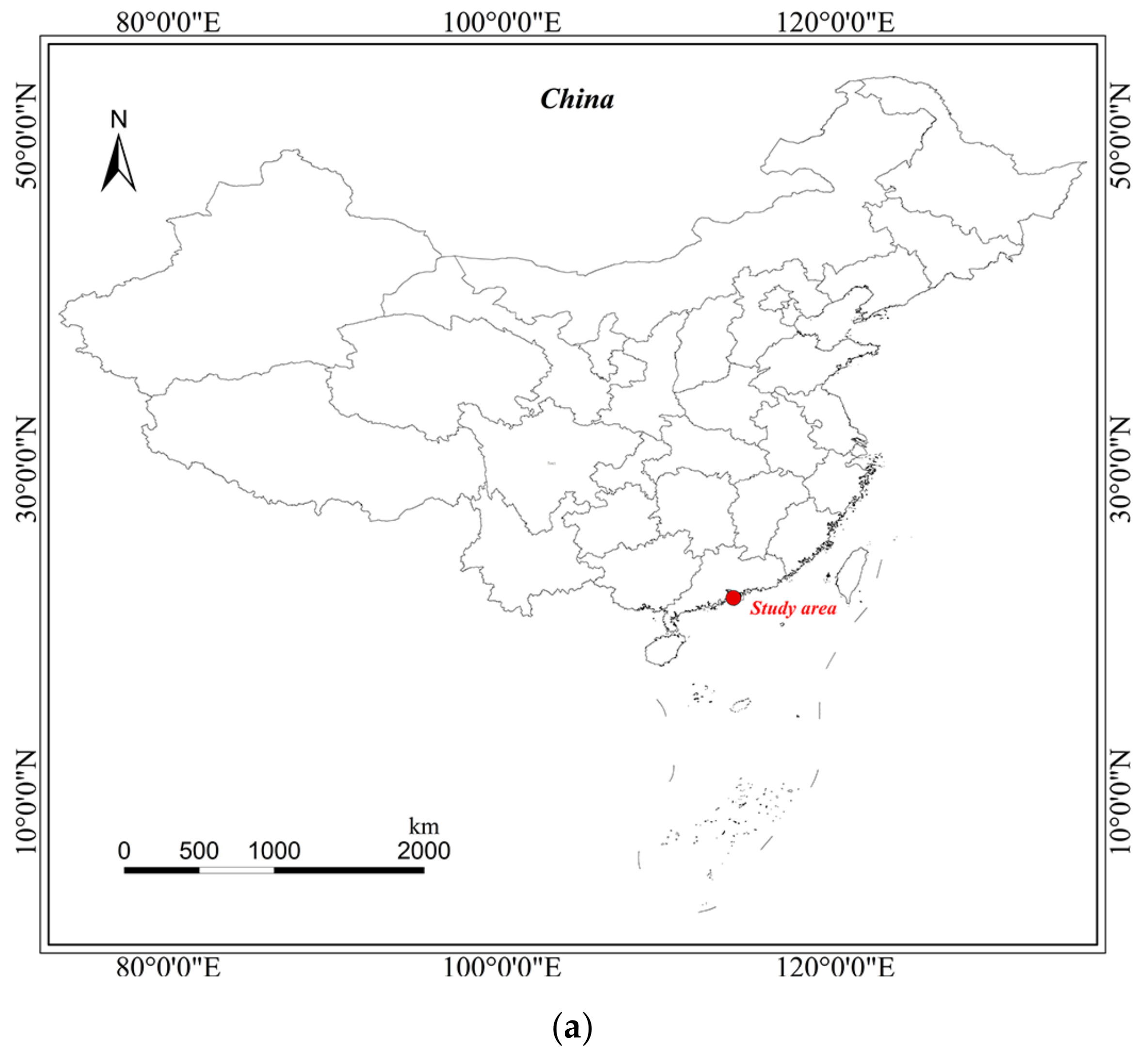
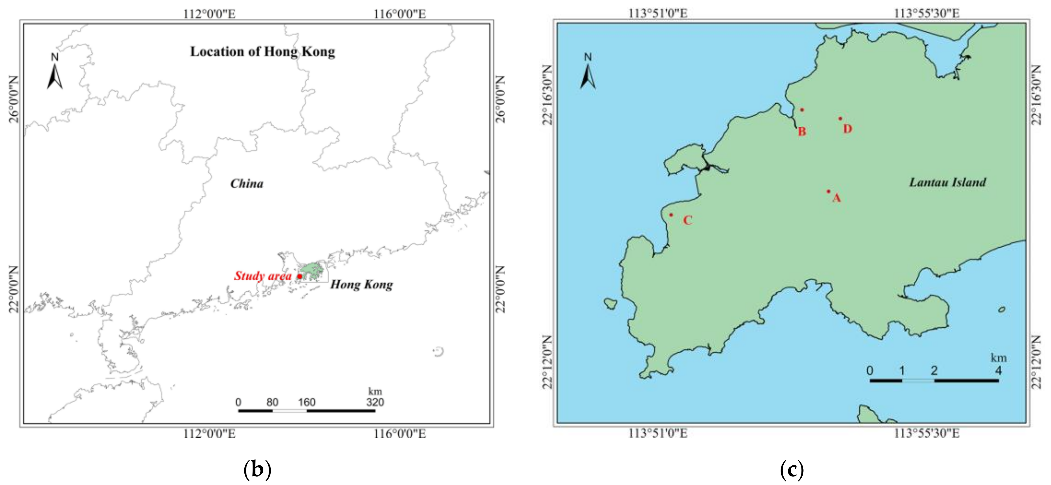
Figure 4.
Study area: (a) China map. (b) The location of Hong Kong. (c) Locations of Datasets A, B, C, and D on Lantau Island, Hong Kong, China.
Figure 4.
Study area: (a) China map. (b) The location of Hong Kong. (c) Locations of Datasets A, B, C, and D on Lantau Island, Hong Kong, China.


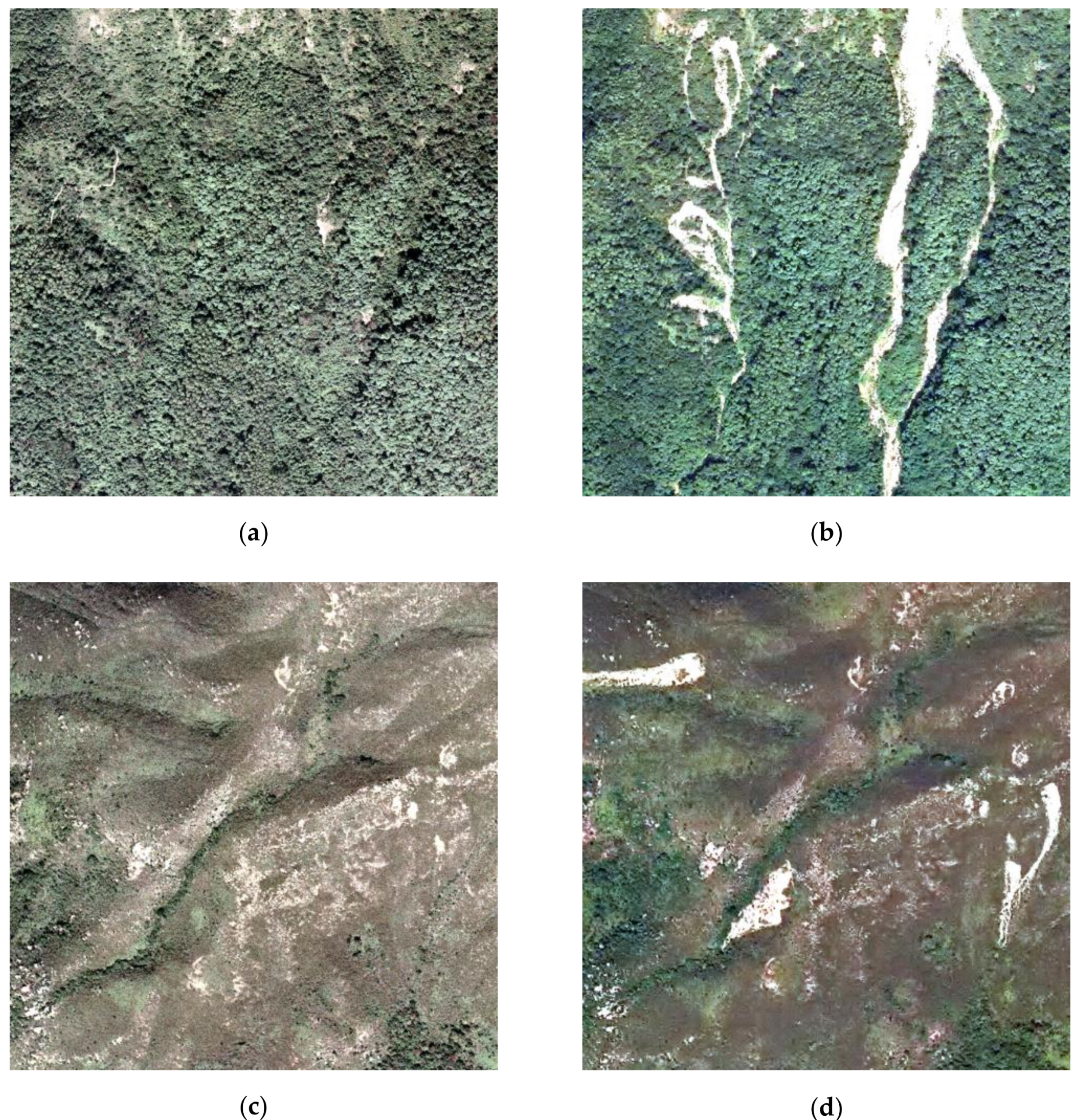
Figure 5.
Datasets used in the experiments: (a,b) Pre- and post-event images of Dataset A; (c,d) Pre- and post-event images of Dataset B; (e,f) Pre- and post-event images of Dataset C; (g,h) Pre- and post-event images of Dataset D.
Figure 5.
Datasets used in the experiments: (a,b) Pre- and post-event images of Dataset A; (c,d) Pre- and post-event images of Dataset B; (e,f) Pre- and post-event images of Dataset C; (g,h) Pre- and post-event images of Dataset D.


Figure 6.
The LM results for Dataset A: (a) Change-detection-based Markov random field (CDMRF); (b) Object-based majority voting (OMV); (c) Superpixel-based difference representation learning (SDRL); (d) Semi-supervised GAN (SGAN); (e) Semi-supervised multi-temporal deep representation fusion network (SMDRF-Net); (f) Ground reference data; (g) Zoom for CDMRF; (h) Zoom for OMV; (i) Zoom for SDRL; (j) Zoom for SGAN; (k) Zoom for SMDRF-Net.

Figure 7.
The LM results for Dataset B: (a) CDMRF; (b) OMV; (c) SDRL; (d) SGAN; (e) SMDRF-Net; (f) Ground reference data; (g) Zoom for CDMRF; (h) Zoom for OMV; (i) Zoom for SDRL; (j) Zoom for SGAN; (k) Zoom for SMDRF-Net.
Figure 7.
The LM results for Dataset B: (a) CDMRF; (b) OMV; (c) SDRL; (d) SGAN; (e) SMDRF-Net; (f) Ground reference data; (g) Zoom for CDMRF; (h) Zoom for OMV; (i) Zoom for SDRL; (j) Zoom for SGAN; (k) Zoom for SMDRF-Net.

Figure 8.
The LM results for Dataset C: (a) CDMRF; (b) OMV; (c) SDRL; (d) SGAN; (e) SMDRF-Net; (f) Ground reference data; (g) Zoom for CDMRF; (h) Zoom for OMV; (i) Zoom for SDRL; (j) Zoom for SGAN; (k) Zoom for SMDRF-Net.
Figure 8.
The LM results for Dataset C: (a) CDMRF; (b) OMV; (c) SDRL; (d) SGAN; (e) SMDRF-Net; (f) Ground reference data; (g) Zoom for CDMRF; (h) Zoom for OMV; (i) Zoom for SDRL; (j) Zoom for SGAN; (k) Zoom for SMDRF-Net.

Figure 9.
The LM results for Dataset D: (a) CDMRF; (b) OMV; (c) SDRL; (d) SGAN; (e) SMDRF-Net; (f) Ground reference data; (g) Zoom for CDMRF; (h) Zoom for OMV; (i) Zoom for SDRL; (j) Zoom for SGAN; (k) Zoom for SMDRF-Net.
Figure 9.
The LM results for Dataset D: (a) CDMRF; (b) OMV; (c) SDRL; (d) SGAN; (e) SMDRF-Net; (f) Ground reference data; (g) Zoom for CDMRF; (h) Zoom for OMV; (i) Zoom for SDRL; (j) Zoom for SGAN; (k) Zoom for SMDRF-Net.

Figure 10.
Relationship between LM accuracy and segmentation scales.

Figure 11.
Relationship between LM accuracy and sample sizes.

Figure 12.
Relationship between LM accuracy and network structures of the critic in the Wasserstein generative adversarial network with gradient penalty (WGAN-GP): (a) Overall Accuracy (OA) and (b) Kappa coefficient (KC).
Figure 12.
Relationship between LM accuracy and network structures of the critic in the Wasserstein generative adversarial network with gradient penalty (WGAN-GP): (a) Overall Accuracy (OA) and (b) Kappa coefficient (KC).


Table 1.
Details of experimental datasets.
| Dataset | The Center Coordinate | Resolution (m) | Size (Pixels) | Acquisition Time | Land Cover Types |
|---|---|---|---|---|---|
| A | 22° 14′ 52′′ N, 113°53′ 52′′ E | 0.5 | 960 × 960 | December 2007 and November 2014 | forests |
| B | 22° 16′ 14′′ N, 113°53′ 24′′ E | 0.5 | 740 × 780 | December 2007 and November 2014 | shrublands and volcanic rocks |
| C | 22° 14′ 28′′ N, 113°51′ 14′′ E | 0.5 | 700 × 700 | December 2005 and November 2008 | dense grasslands and sparse woodlands |
| D | 22° 16′ 06′′ N, 113°54′ 05′′ E | 0.5 | 600 × 600 | December 2005 and November 2008 | sparse shrublands and grasslands with some rocks |
Table 2.
Quantitative comparison between the methods used for comparison and the proposed approach (numbers are bolded).
Table 2.
Quantitative comparison between the methods used for comparison and the proposed approach (numbers are bolded).
| Dataset | Method | CP | CR | QA | KC | OA |
|---|---|---|---|---|---|---|
| A | CDMRF | 0.48 | 0.78 | 0.42 | 0.57 | 95.03% |
| OMV | 0.89 | 0.69 | 0.64 | 0.76 | 96.15% | |
| SDRL | 0.70 | 0.83 | 0.61 | 0.74 | 96.63% | |
| SGAN | 0.64 | 0.82 | 0.56 | 0.70 | 96.19% | |
| SMDRF-Net | 0.91 | 0.83 | 0.76 | 0.85 | 97.54% | |
| B | CDMRF | 0.74 | 0.84 | 0.65 | 0.79 | 99.17% |
| OMV | 0.92 | 0.70 | 0.66 | 0.79 | 99.02% | |
| SDRL | 0.71 | 0.93 | 0.67 | 0.80 | 99.27% | |
| SGAN | 0.71 | 0.91 | 0.66 | 0.79 | 99.23% | |
| SMDRF-Net | 0.90 | 0.92 | 0.83 | 0.90 | 99.59% | |
| C | CDMRF | 0.60 | 0.85 | 0.55 | 0.69 | 97.54% |
| OMV | 0.94 | 0.71 | 0.68 | 0.80 | 97.79% | |
| SDRL | 0.80 | 0.83 | 0.69 | 0.81 | 98.22% | |
| SGAN | 0.60 | 0.88 | 0.56 | 0.70 | 97.57% | |
| SMDRF-Net | 0.85 | 0.91 | 0.78 | 0.87 | 98.83% | |
| D | CDMRF | 0.81 | 0.83 | 0.70 | 0.81 | 98.29% |
| OMV | 0.94 | 0.70 | 0.67 | 0.79 | 97.76% | |
| SDRL | 0.93 | 0.75 | 0.71 | 0.82 | 98.20% | |
| SGAN | 0.73 | 0.91 | 0.68 | 0.80 | 98.32% | |
| SMDRF-Net | 0.92 | 0.85 | 0.80 | 0.86 | 98.84% |
Publisher’s Note: MDPI stays neutral with regard to jurisdictional claims in published maps and institutional affiliations. |
© 2021 by the authors. Licensee MDPI, Basel, Switzerland. This article is an open access article distributed under the terms and conditions of the Creative Commons Attribution (CC BY) license (http://creativecommons.org/licenses/by/4.0/).
Share and Cite
MDPI and ACS Style
Zhang, X.; Pun, M.-O.; Liu, M. Semi-Supervised Multi-Temporal Deep Representation Fusion Network for Landslide Mapping from Aerial Orthophotos. Remote Sens. 2021, 13, 548. https://0-doi-org.brum.beds.ac.uk/10.3390/rs13040548
AMA Style
Zhang X, Pun M-O, Liu M. Semi-Supervised Multi-Temporal Deep Representation Fusion Network for Landslide Mapping from Aerial Orthophotos. Remote Sensing. 2021; 13(4):548. https://0-doi-org.brum.beds.ac.uk/10.3390/rs13040548
Chicago/Turabian StyleZhang, Xiaokang, Man-On Pun, and Ming Liu. 2021. "Semi-Supervised Multi-Temporal Deep Representation Fusion Network for Landslide Mapping from Aerial Orthophotos" Remote Sensing 13, no. 4: 548. https://0-doi-org.brum.beds.ac.uk/10.3390/rs13040548
Note that from the first issue of 2016, this journal uses article numbers instead of page numbers. See further details here.