
Spatial Interconnections of Land Surface Temperatures with Land Cover/Use: A Case Study of Tokyo


1
Graduate School of Life and Environmental Sciences, University of Tsukuba, 1-1-1 Tennodai, Tsukuba, Ibaraki 305-8572, Japan
2
Institute of Remote Sensing and Earth Sciences, Hangzhou Normal University, Yuhangtang Road No.2318, Hangzhou 311121, China
3
Faculty of Life and Environmental Sciences, University of Tsukuba, 1-1-1 Tennodai, Tsukuba, Ibaraki 305-8572, Japan
*
Author to whom correspondence should be addressed.
Remote Sens. 2021, 13(4), 610; https://0-doi-org.brum.beds.ac.uk/10.3390/rs13040610
Submission received: 30 December 2020
/
Revised: 28 January 2021
/
Accepted: 3 February 2021
/
Published: 8 February 2021
(This article belongs to the Section Urban Remote Sensing)
Abstract
:As one of the most populated metropolitan areas in the world, the Tokyo Metropolitan Area (TMA) has experienced severe climatic modifications and pressure due to densified human activities and urban expansion. The surface urban heat island (SUHI) phenomenon particularly constitutes a significant threat to human comfort and geo-environmental health in TMA. This study aimed to profile the spatial interconnections between land surface temperature (LST) and land cover/use in TMA from 2001 to 2015 using multi-source spatial data. To this end, the thermal gradients between the urban and non-urban fabric areas in TMA were examined by joint analysis of land cover/use and LST. The spatiotemporal aggregation patterns, variations, and movement trajectories of SUHI intensity in TMA were identified and delineated. The spatial relationship between SUHI and the potential driving forces in TMA was clarified using geographically weighted regression (GWR) analysis. The results show that the thermal environment of TMA exhibited a polynucleated spatial structure with multiple thermal island cores. Overall, the magnitude and extent of SUHI in TMA increased and expanded from 2001 to 2015. During that time, SUHIs clustered in the compact residential quarters and redevelopment/renovation areas rather than downtown. The GWR models showed better performance than ordinary least squares (OLS) models, with Adj R2 > 0.9, indicating that the magnitude of SUHI significantly depended on its neighboring geographical setting, including land cover composition and configuration, population size, and terrain. We suggest that UHI mitigation in Tokyo should be focused on alleviating the magnitude of persistent thermal cores and controlling unstable SUHI occurrence based on partitioned or location-specific landscape design. This study’s findings have immense implications for SUHI mitigation in metropolitan areas situated in bay regions.
1. Introduction
In the 21st century, tackling climate change is arguably considered the top priority to ensure human comfort and geo-environmental health [1]. The Intergovernmental Panel on Climate Change (IPCC) and the United Nations (UN) Framework Convention on Climate Change (FCCC) has emphasized the importance of addressing urban climate issues and enumerated the enormous consequences [2,3], such as global warming, weather extremes, etc. In particular, due to densified human activities and intensified urban sprawl, the climate crisis in the urban context is continuously amplified [4]. Urban areas have experienced overwhelming risks and pressures [5,6]. The underlying mechanisms and processes of the urban thermal–energy system are thereby altered, and the urban heat island (UHI) effect is gradually generated [7]. The UHI phenomenon is driven by surface temperature cliffs between urban and non-urban areas [8,9,10,11]. In light of this, extremely high temperatures in populated urban areas, in contrast with their surrounding rural spaces, have been a severe climatic threat [11,12]. The UN projected that more than two-thirds of the world population would dwell in urban areas by 2050 [13,14]. These people would be exposed to high-temperature anomalies as well.
As one of the most vibrant, populated, and livable regions across the globe, the Tokyo Metropolitan Area (TMA) has been struggling to overcome the problems caused by urban expansion and extreme climate events since the adoption of the Kyoto Protocol (1997) [15,16,17,18,19]. As of 2015, the population of Tokyo reached 9.273 million, and the growth rate reached 14% compared with 2000 [20]. With a population density of 6169 persons per km2, Tokyo is home to 11% of Japan’s total population but only covers less than 1% of the total area of the country [21]. The increase in population is mirrored by urgent demands for urban services and environmental supply. Thus, it is vital to foster a sustainable Tokyo, which contributes to a vigorous metropolitan area that embraces ecological harmony and economic prosperity. As Japan’s central locus, Tokyo has always been struck by the UHI effect due to drastic metropolization, and it has acquired a series of problems, such as increased urban energy consumption, increased greenhouse gas emissions, and deteriorated urban air quality [22]. The centennial increment of Tokyo’s annual average temperature was estimated at approximately 3 ℃ by the Japan Meteorological Agency (JMA) [23,24,25,26]. Records of unseasonable high-temperature days/nights in Tokyo have been soaring [27,28]. Out-of-control UHI could wipe out hard-won gains for the urban environment and human health. Therefore, alleviating the UHI effect is highlighted as one of the most prominent challenges in Tokyo. Evaluating the evolutionary track of the urban thermal environment in Tokyo and UHI mitigation strategies yields experiences and lessons for other expanding metropolitan areas in bay regions.
Since the 2000s, the Tokyo Metropolitan Research Institute for Environmental Protection (TMRIEP) has set up massive meteorological observation frameworks in order to expand UHI investigations [25,29]. Plentiful and valuable findings on urban/suburban atmospheric heat conditions in Tokyo have been obtained from high-spatial-density monitoring stations [25,27,30]. This kind of canopy-layer UHI (CUHI) investigation based on isolated meteorological stations has contributed to UHI mitigation initiatives. Assessments of CUHI have identified the thermal impacts on specific locations over time using absolute atmospheric temperature. However, they ignored the spatial heterogeneity of UHI due to sparsely distributed in situ measurements [10]. In contrast, by estimating land surface temperature (LST), satellite-derived surface UHI (SUHI) monitoring at various spatiotemporal resolutions replenishes large-scale and long-term UHI observations. Satellite thermal infrared (TIR) remote sensing data, such as Landsat constellation and Moderate Resolution Imaging Spectroradiometer (MODIS) archives, have been extensively utilized for surface temperature measurement due to their short revisit intervals and broad spatial coverage [10,31].
Unlike in situ atmospheric temperature measurements, retrieved LST using Landsat data provides an in-depth evaluation of the thermal situation and surface parameter responses in the high spatial-sensitive context [8,10,31,32]. Together with various ecological, environmental, and socioeconomic parameters, the detailed information of radiative surface temperature can be interpreted to study underlying surface conditions and interactions between atmospheric circumstances and human activities [10]. Until recently, an incredible number of UHI-related scientific studies based on Landsat satellite data have explored the linkages between SUHI and its potential driving force from urbanization [10,31,33,34,35,36,37,38,39,40]. Deilami et al. [41] identified the association between SUHI and land cover patterns in Brisbane based on spatial regression models at comparative cross-sectional and longitudinal perspectives. They found that the influences of population density and porosity vary significantly over space. Li et al. [42] depicted the spatiotemporal patterns of SUHI in Hangzhou and confirmed that increasing population and green space substantially affect changes in SUHI. Liu et al. [43] evaluated the impact of land cover/use on SUHI for 10 Chinese megacities and demonstrated that the land cover composition and the population had notable effects on altering the intensity of SUHI. Wang et al. [44] simulated land use/cover scenarios and impacts on land surface temperature in Sapporo and stated that urban expansion was the main driver affecting SUHI. Wang et al. [45] investigated the connections among urban landscape, population, and LST in three megacities along the Yangtze River (Chongqing, Nanjing, and Wuhan) and concluded that the effects of landscape composition and configuration on LST differed across cities.
However, few studies have depicted the spatiotemporal evolution of thermal gradients in Tokyo based on Landsat monitoring. The spatiotemporal interconnections between SUHI and its urbanization-induced influencing factors in Tokyo have also been scarcely interpreted due to the complicated urban setting. Tokyo’s urban areas are contiguous with each other or border on urban fringes or suburban areas rather than rural areas. It is challenging to delineate and harmonize the contours of UHIs without knowing the distinct temperature differences between typical urban and rural sectors. Although several studies effectively identified the spatial patterns and characteristics of the thermal environment in Tokyo [46,47,48], the temporal dynamic component of land cover/use on LST in Tokyo was disregarded. Furthermore, the thermal environment mechanism is complicated [8,49,50] and impacted by mixed factors [10,31]. In light of this, interpreting the evolution of Tokyo’s thermal environment requires a novel investigation into the dynamism of diverse underlying factors. In this context, a more comprehensive assessment of Tokyo’s thermal environment is required in order to provide in-depth insights into the spatiotemporal dynamics of the influencing factors on urban thermal comfort. In addition, profiling how Tokyo has managed heat islands through urban planning can enrich the knowledge of urban sustainability and contribute to urban climate responses in the broader international context.
Hence, this study’s chief objective was to conduct an integrative assessment of spatial interconnections between LST and land cover/use using multi-source long-term remote sensing data in Tokyo. The second objective was to capture and characterize the spatiotemporal variations and trends of the urban thermal environment for comfort and sustainability. We intend to provide a cross-sectional and longitudinal investigation that permits spatiotemporal evaluations of Tokyo’s thermal environment based on land cover/use scenarios, coupled with remotely sensed data from multiple sources and spatial statistical analysis. This study’s findings can support the validity of the analytical approaches undertaken and the universality of the research process for other metropolitan areas at the national and global scale, such as Osaka, Fukuoka, Shanghai, Hong Kong, Singapore, Los Angeles, etc.
2. Study Area and Methods
2.1. Study Site
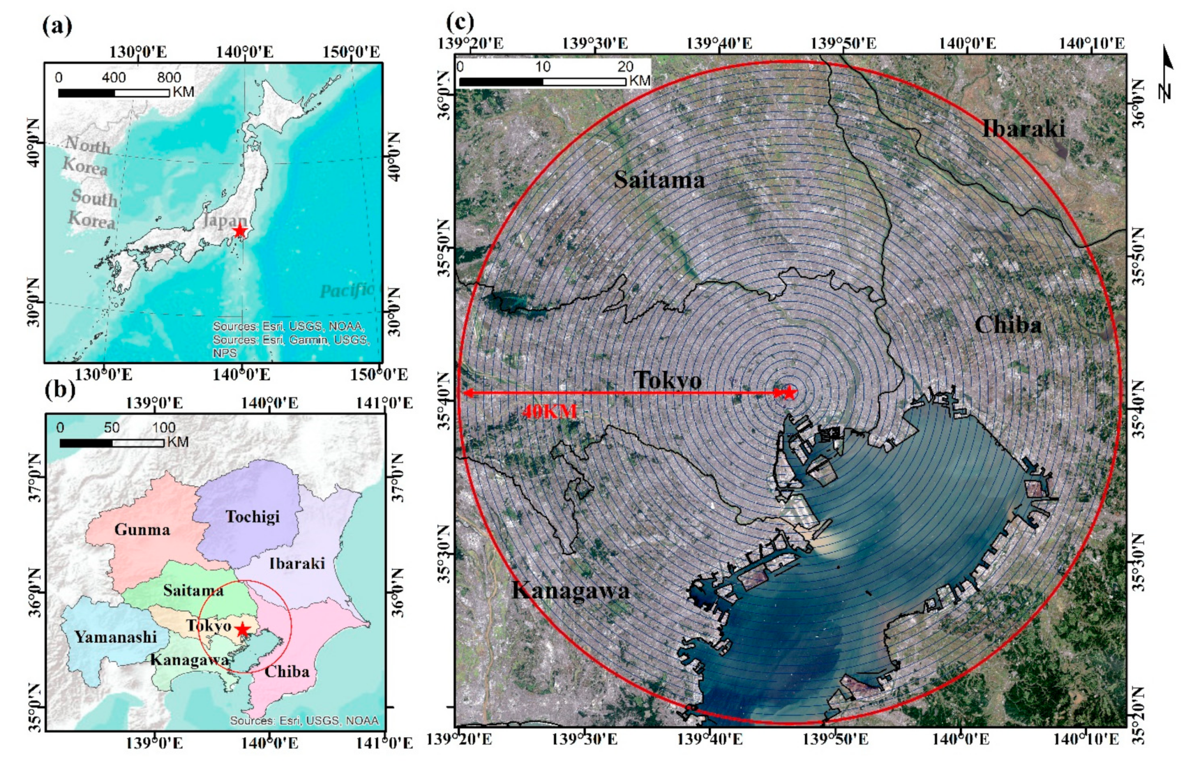
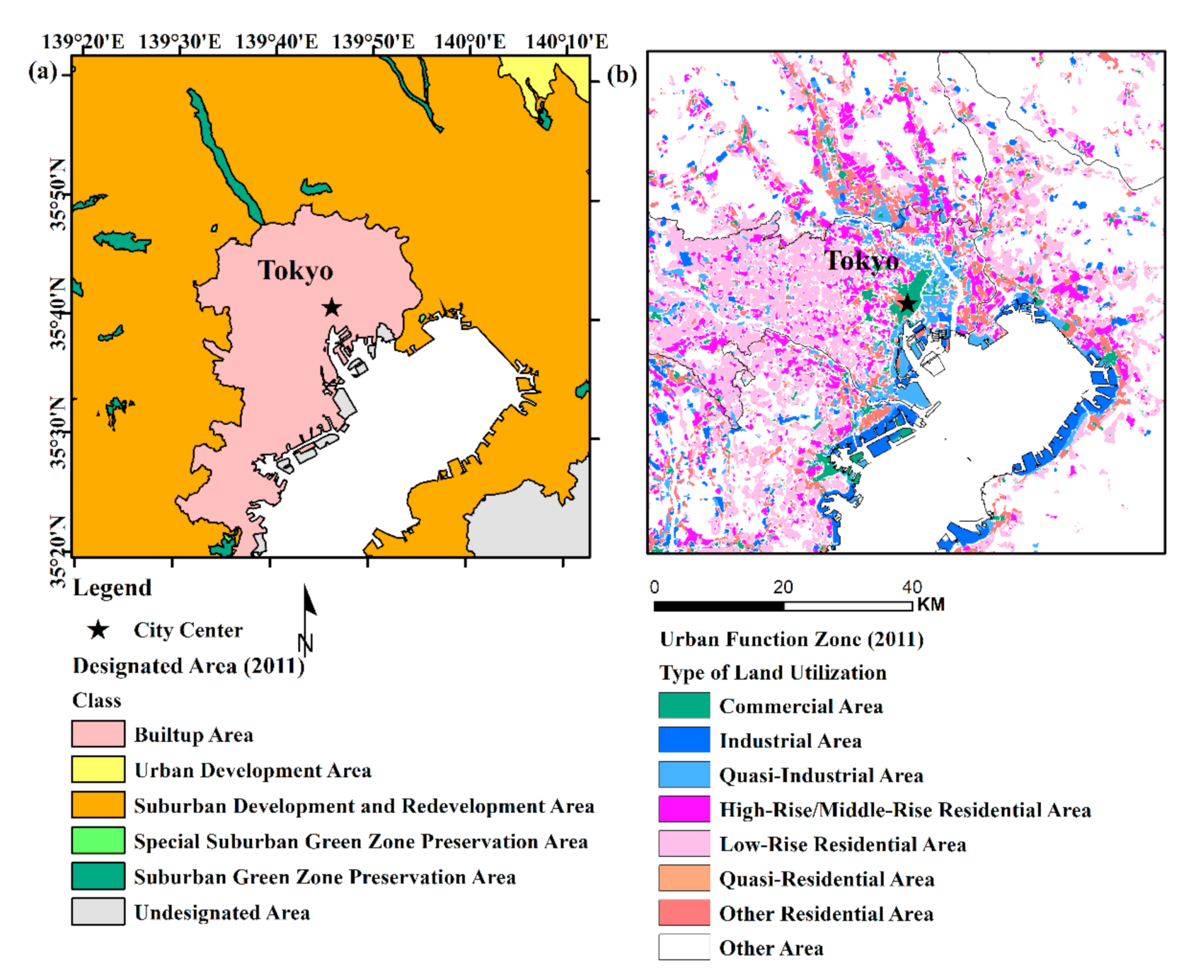
This study was conducted in the context of the Tokyo Metropolitan Area (TMA), Japan. We focused on the landscape and its influence on LST within a radius of 40 km from Tokyo Station (the city center; latitude: 35°40′51″N; longitude: 139°46′1″E), as shown in Figure 1. This area encompasses most of the urban–suburban–rural areas in Tokyo with many land details. More than 37 million people reside in the TMA [20]. Due to speedy urbanization, the TMA is a representative region of Japan and the world. The substantial settlement agglomerations and urban infrastructure constructions in TMA have given rise to urban warming and contributed to the climate crisis [25,26]. Under the climate scheme, TMA is situated in a humid subtropical zone with a complex aggregation of diverse land covers/uses. Consequently, TMA experiences hot and humid weather from May to early October. In recent decades, TMA has been subjected to frequent severe high temperatures in summer and autumn. The highest recorded temperature ranged between 34.2 °C and 39.5 °C from 2001 to 2015 [20]. This increased tropical weather resulted in a surge of heat-related health problems and destroyed the balance of the thermal environment.
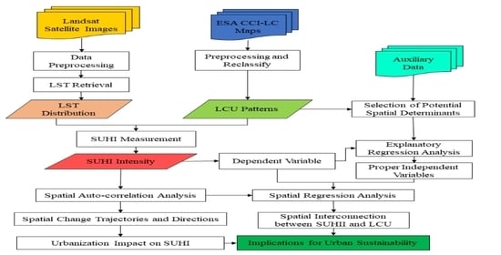
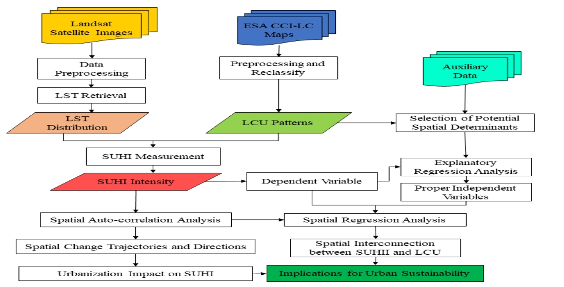
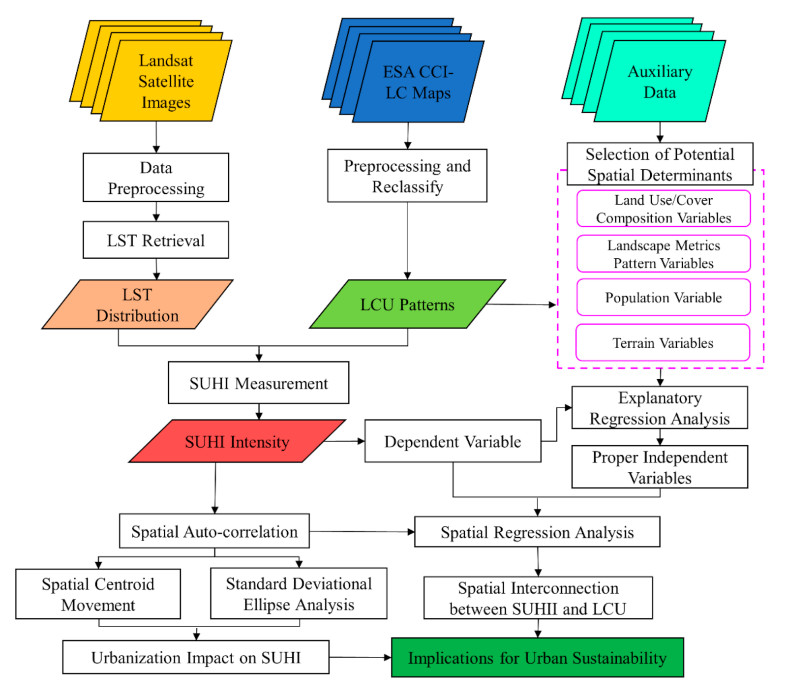
2.2. Working Flowchart
This study used multi-source spatial data to examine the causal mechanism and associations between LST and land cover in TMA based on cross-sectional and longitudinal spatial regression models. The overall technical processing scheme is shown in Figure 2.
2.3. Land Cover/Use Specifications
In this study, land cover/use thematic maps of TMA were obtained from the global land cover (LC) products of the European Space Agency (ESA) Climate Change Initiative (CCI) [51]. The annual CCI-LC products at 300-m spatial resolution have been treated as persuasive data in a broad range of LC-related research [51,52]. The CCI-LC classification scheme is defined as 37 hierarchical categories, including 22 global and 15 regional classes based on the Land Cover Classification System (LCCS). The LCCS, developed by the UN (http://www.fao.org/docrep/003/x0596e/x0596e00.HTM), delivers great LC details and has flexibility in adjusting the thematic legend in order to serve diverse applications. The validation framework of CCI-LC products was established globally on international standards, using both the pixel-based uncertainty value and object-based expert verification of 2600 primary sampling units. The overall weighted-area accuracy of the CCI-LC 2015 product is assessed to be 71.1% [51].
The thematic details in TMA were extracted from global LC maps and rectified to northern Universal Transverse Mercator map projection zone 54 (UTM zone 54N). The LC thematic legend was rearranged into five categories considering TMA’s urban setting and land use utilization together with SUHI profiling—agricultural land (AL), forest land (FL), mixed land (ML), urban fabric (UF), and water area (WA). The specifications of TMA’s LC legend are shown in Table 1. Time series CCI-LC LC maps of 2001, 2006, 2013, and 2015 were exploited in this study based on the time correspondence of other data. The reprocessed LC maps were then used to compute the landscape pattern metrics based on the landscape-level moving window in FRAGSTATS 4.2 developed by the University of Massachusetts, making it possible to quantify the relationship between the configuration of land cover/use and LST in the context of spatial heterogeneity [53].
2.4. LST Retrieval and SUHI Assessment
The multitemporal Landsat constellation images of TMA (Landsat collection 1 Level 2 (On-Demand); path: 107, row: 35) were utilized in this study. All Landsat scenes were geometric-corrected, radiometric-calibrated, and atmospheric-corrected by the United States Geological Survey (USGS; https://earthexplorer.usgs.gov/). The corresponding image products were also retrieved, including multispectral surface reflectance, spectral indices, and atmospheric brightness temperature in Kelvin (K). Considering the availability and comparability of data, time-series Landsat data in the same season (autumn in this study) or within three-month intervals were given priority. The selected images were cloud-free or had minimum cloud cover (<10%). In addition, the local hourly meteorological data archives from the JMA were used to confirm the existence of extreme weather factors in the 24 h before and after image acquisition. Based on these considerations, we utilized Landsat data from 24 September 2001, 16 October 2006, 17 September 2013, and 9 October 2015 in this study.
Initially, LST was the primary indicator to capture the spatiotemporal pattern of SUHI in TMA. Many studies have provided detailed descriptions of radiative transfer equation (RTE)-based LST retrieval using Landsat thermal bands [36,54,55]. The RTE can be expressed as Equation (1). Briefly, RTE-based LST retrieval involves three main procedures: (1) convert Landsat digital numbers (DNs) to top of atmosphere (ToA) radiance, (2) calculate at-sensor brightness temperature (BT), and (3) compute LST [56,57].
where is Landsat spectral ToA radiance at the wavelength , with as the measurement unit; is Planck’s law-defined equivalent blackbody radiance () at temperature T in Kelvin (K) and wavelength in ; is the atmospheric transmissivity of Landsat sensor-land surface, unitless; is land surface emissivity at the wavelength , unitless, and was estimated based on fractional vegetation proposed by Sobrino et al. [56] through the normalized difference vegetation index (NDVI) threshold method; is upwelling atmospheric radiance, with as the measurement unit; and is downwelling atmospheric radiance, with as the measurement unit.
Three important parameters can be obtained from the module of atmospheric correction by NASA (https://atmcorr.gsfc.nasa.gov) [57,58,59]—atmospheric transmissivity (), upwelling radiance (), and downwelling radiance (). The details of thermal image information and atmospheric parameters are shown in Table 2.
LST-related studies are often highly climate-sensitive, and the investigated results are sensitive to the weather effect [42,43]. The responses of LST values are varied and complicated at different locations and dates. The evolution of the thermal environment in different phases should be investigated using the same statistical frame and harmonized legend. Although the selected Landsat images in this study were within the same season, it is meaningless and inappropriate to directly compare the spatiotemporal variations of the thermal environment for periods using absolute LST values due to enormous uncertainty and bias. Therefore, instead of absolute LST observations, spatiotemporal patterns of SUHI intensity were utilized in this study for analyzing and comparing the evolution of TMA’s thermal environment. The intensity of SUHI (SUHII) was measured by the estimated LST differences in urban/rural areas. The extrema of LST values were removed to eliminate uncertainty and errors in LST retrieval, making the temperature information comparable. The generated LST values were normalized to the range of 0–1 using the min–max rescaling method. For estimated LST values, the minimum and maximum values of LST were transformed into 0 and 1, respectively; the other LST values were rescaled into a decimal between 0 and 1 [43,54]. Herein, SUHII was computed as Equation (2), which subtracts the mean temperature value of non-urban area (non-UF category pixels) from the temperature value of each pixel in the study region [43,60,61] as follows:
where and are the LST values of urban and rural pixels, respectively; is the LST value of pixel i within the study region; and denotes the mean LST value of non-UF pixels. UF category pixels are substituted for urban pixels, while non-urban pixels contain the pixels of other land cover/use categories (AL, ML, FL, and WA).
2.5. Spatial Aggregation Pattern and Variations of SUHI
Since the adverse effect of SUHI is a consequence of urban sprawl and human activities over time [8,11,31,62], the relationship between the urban thermal environment and urbanization needs to be highlighted and interpreted to delineate the spatial clustering pattern of SUHII [42]. The variations in the spatiotemporal aggregations of SUHII in TMA mirror the evolution of the urban spatial layout from different angles. Herein, Moran’s I (MI) [42,63] was computed to reflect the geographic pattern of TMA’s thermal environment on a global scale (Equation (3)) as follows:
where n is the total number of spatial analytical units, is the mean SUHII value for spatial unit i, denotes the spatial weight between spatial units i and j, and represents the mean SUHII value within the whole study area. The SUHI data were conceptualized and structured through spatial sparse weight matrix techniques. Using the inverse distance weighted strategy, the neighboring features were varied and influential, and spatial weights were computed to reflect the variations of the thermal environment. When the global thermal pattern of TMA is spatially autocorrelated, the occurrence of positive MI hints at spatial clusters of high or low SUHII values; conversely, negative MI implies a spatial dispersion of high and low SUHII values. In the case that MI has a value of 0, the global thermal pattern is spatially random.
This study also adopted hot spot analysis to delineate the local spatial aggregations of SHUII in TMA based on Getis-Ord Gi* spatial statistics. The calculation of the Getis-Ord local statistic () is based on Equation (4) [63,64] as follows:
where n is the total number of spatial analytical units, denotes the SUHII value for spatial unit j, and S indicate the mean and variance of SUHII values within the whole study area, respectively, and is the spatial weight between i and j.
The tool for hot spot analysis in ArcGIS 10.4, developed by Environmental Systems Research Institute (ESRI), was employed to estimate the Getis-Ord Gi* statistic for each spatial analytical unit of the SUHII data. The existence and locations of local clusters with statistically significant for a specified distance were identified spatially by the results of (Table 3). This step was conducted by looking at each grid in the context of spatial neighbors. In terms of statistical significance, a larger and positive represents a significant hot spot that has more intense local clustering of high SUHII values, while a smaller and negative signifies a significant cold spot that has more intense local clustering of low SUHII values. When the approaches zero, it indicates the absence of apparent spatial clustering on the local scale. A confidence level of 90% or higher was utilized in further analysis.
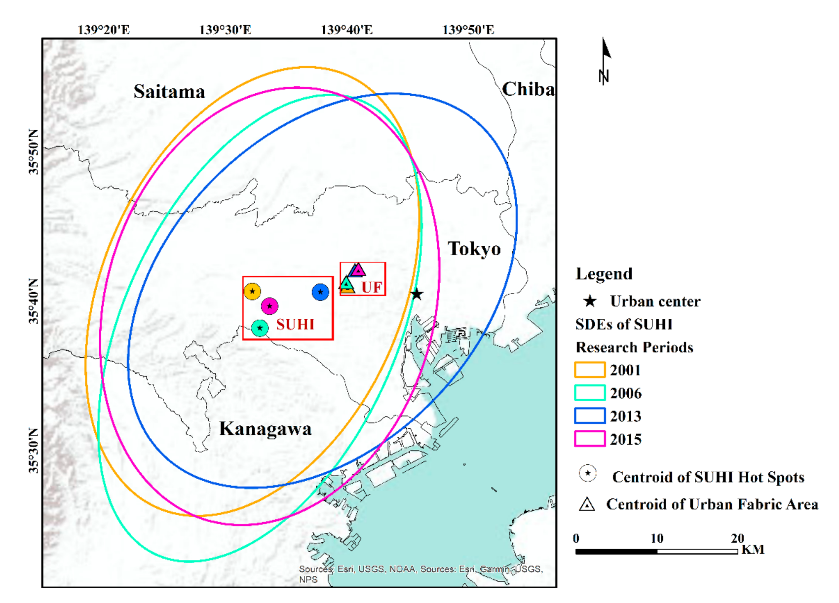
Additionally, the spatial centroid [65,66], together with standard deviational ellipse (SDE) [67,68] analysis, was implemented to explore the response of the thermal environment to the evolution of the urban landscape. The methodological details of centroid coordinates and SDE parameters can be found in Xu et al. [69] and Johnson et al. [70]. The spatial centroid movement of SUHI hot spots in 2001, 2006, 2013, and 2015 was calculated for a hint at the evolutionary trajectory of TMA’s urban thermal environment. The UF centroids in the corresponding years were created to indicate the direction and track of urban expansion in TMA during the research periods. Based on the spatial pattern of SUHI hotspots, SUHII weighted SDEs across time series were also calculated to enhance our understanding of the spatiotemporal dynamic processes of TMA’s urban thermal environment.
2.6. Spatial Regression Analysis
2.6.1. Geographically Weighted Regression Analysis
Linear regression analysis is intended to signify a dependent variable by a suite of independent variables with a linear weight combination [38,71,72,73,74]. Referring to the issues of spatial non-stationarity and location independency, many studies, particularly those concerning geography and climatology [71,72,75], have shown that the geographically weighted regression (GWR) model is more precise and appropriate for quantifying the relations between dependent and independent variables than conventional regression models (e.g., ordinary least squares (OLS)) [41,72,76,77]. For instance, Zhao et al. [76] examined the relationship between SUHI and underlying biophysical factors in Austin and San Antonio, Texas, using (and comparing) OLS and GWR models, indicating the non-stationary spatial effect of relevant underlying biophysical factors on SUHI. Li et al. [72] assessed the relationships between diurnal/seasonal SUHI and underlying drivers in 419 major cities all over the world using the GWR model and compared the results to global regression models. Thus, recently, GWR is being utilized more to mirror spatial heterogeneity and geographical connections [10]. In GWR, the complicated spatially varying relationships of dependent and independent variables can be estimated and simulated using a locally linear form of a parameter matrix, which can be expressed mathematically as [41,43,72,74,76]
where i indicates the location of a dependent variable (mean SUHII) for each spatial unit, labeled as the coordinate ; k represents the number of explanatory variables (driving forces) within a spatial unit, ,, and stand for the values of the dependent variable, the kth explanatory variable, and the random disturbance for spatial unit i, respectively; and and represent the estimates of the intercept parameter and the local regression coefficient for the kth explanatory variable for spatial unit i, respectively.
The performance of the GWR model is sensitive to spatial kernel functions and the bandwidth statistical method. A set of evaluation parameters was computed based on ArcGIS 10.4 and RStudio for verifying the reliability and accuracy of the model, including the coefficient of determination (R2), corrected Akaike information criterion (AICc), MI of the residuals, variance inflation factor (VIF), F-test, etc.
2.6.2. Selection of Spatial Determinants
The interconnections between SUHII and its influencing factors in TMA were clarified and highlighted using spatial regression analysis (OLS and GWR). Thus, the average SUHII of each spatial analytical unit was calculated as the dependent variable. Prior knowledge suggests that an array of potential explanatory variables can be considered [41,43,76,77,78]. The candidates for explanatory variables are listed by type as follows:
- (1)
- Land cover/use composition variables—In terms of land cover/use composition, the proportion of urban fabric area (UFP), normalized difference built-up index (NDBI), forest proportion (FP), normalized difference vegetation index (NDVI), and water proportion (WP) were considered as candidate explanatory variables. UFP, FP, and WP came from the UF and FL categories of reprocessed CCI-LC layers. NDVI and NDBI were calculated using Landsat multispectral images;
- (2)
- Landscape metric pattern variables—Determining the size, morphology, and spatial arrangement of urban landscapes is vital to explain urban temperature anomalies. Here, four landscape metric parameters were chosen to quantify the characteristics of diversity, aggregation, and evenness in urban landscapes: Shannon’s diversity index (SHDI), contagion index (CONTAG), patch density (PD), and patch richness (PR). Raster maps of landscape metrics were involved in further tests of explanatory regression;
- (3)
- Population variable—Population or population density indirectly affects the urban thermal field. Along with the vast production of anthropogenic heat, the concentration and overcrowding of the population impose serious pressure and demands on urban settlements and infrastructure constructions. This is why we incorporated the population as one of the essential determinants of SUHI formation. In this study, we used spatial demographic data at a high resolution of 100 m provided by the WorldPop Project, University of Southampton, UK (https://www.worldpop.org/) [79], to map the population distribution in TMA in 2001, 2006, 2013, and 2015. Numerous studies have gained valuable findings using this population data archive [80,81];
- (4)
- Terrain variables—The urban terrain is an important influencing factor of the stark temperature difference between urban and rural zones. Fluctuations of the topography alter the intensity of solar radiation and the thermal properties of surface materials. Here, elevation, slope, and aspect were included as potential explanatory variables. The elevation data at 3 arc-second resolution were extracted from the digital elevation model (DEM) archives of USGS’s Shuttle Radar Topography Mission (SRTM) [82]. Slope and aspect are calculated in ArcGIS based on the elevation.
Subsequently, for each analytical unit, the mean values of the dependent and explanatory variables were extracted and featured as spatial attributes. All data can be aggregated to perform spatial regression analysis.
2.6.3. Implementation of Spatial Regression Model
Regarding spatial regression, we generated a set of 1000 m1000 m grid cells as the appropriate analytical scale for observation. At an analytical scale of 1000 m, the spatial regression analysis can retain sufficient spatial information and weaken the scope of spatial dependence and autocorrelation, according to the findings of previous studies [43,83].
Initially, we carried out an exploratory regression analysis to determine the specific OLS model, examining all possible combinations of candidate explanatory variables that could best interpret the SUHI effect without a multicollinearity problem. The redundancy, model completeness, variable significance, bias, and OLS performance were all diagnosed and described in order to refine the initial OLS model. The final OLS model was determined and implemented with a range of independent variables, consisting of CONTAG, elevation, population density, UFP, and FP.
In this study, both cross-sectional comparison (OLS and GWR models) and longitudinal investigation (time sequence GWR models) were designed and performed. Ultimately, all spatial regression models were tested to determine the overall model fit, residuals, and improvement of GWR over OLS, with ANOVA. It is expected to verify the superiority of the GWR model in predicting the SUHI effect with underlying urban biophysical determinants over conventional regression models. On the other hand, time sequence GWR investigations provided a plausible explanation for accessing the relationship between land cover/use changes and variations in the magnitude of the SUHI effect.
3. Results
3.1. Spatiotemporal Characteristics of Tokyo’s Urban Landscapes and Thermal Environment
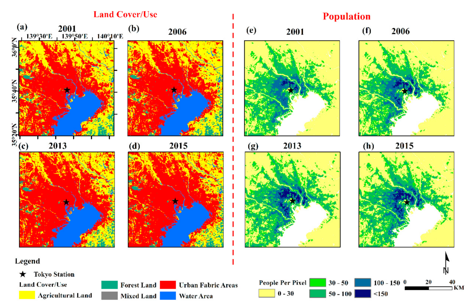
The spatiotemporal evolution of land utilization and thermal environment in TMA was primarily investigated for 2001–2015. The 16 thematic maps (Figure 3 and Figure 4), including land cover/use conversions, population distributions, LST patterns, and SUHI dynamics in 2001, 2006, 2013, and 2015, provided valuable insight into the dynamism and evolution of urban development and the urban thermal environment in TMA since the start of the 21st century. Substantial alterations and transformations of land cover/use layout and configuration took place over those 15 years, especially the expansion of urban artificial landscapes. The UF category was the dominant receiver of land from other land cover/use types. In contrast, AL and FL were significant land providers for urban expansion. Overall, the proportion of UF reached 47.8% in 2015 from 38% in 2001, expanding by nearly a quarter (25.8%) during the 15 years. On the other hand, due to the proliferation of impervious surfaces (IS), the agricultural land area shrunk from 38.1% in 2001 to 29.3% in 2015. Meanwhile, the forest area lost 6.78% of coverage. The magnitude of water area and mixed land underwent less change than other land types between 2001 and 2015. The ever-growing urban artificial coverage led to changes in the urban population and infrastructure. The mean population density of the study area grew by 9.43% between 2001 and 2015. The maximum gridded population density increased by 8.08% between 2001 and 2006, and 6.99% between 2006 and 2015. Geographically, the variations of TMA’s population were primarily concentrated within a 20–30 km zone. These changes were attributed to an accelerating degree of urbanization.
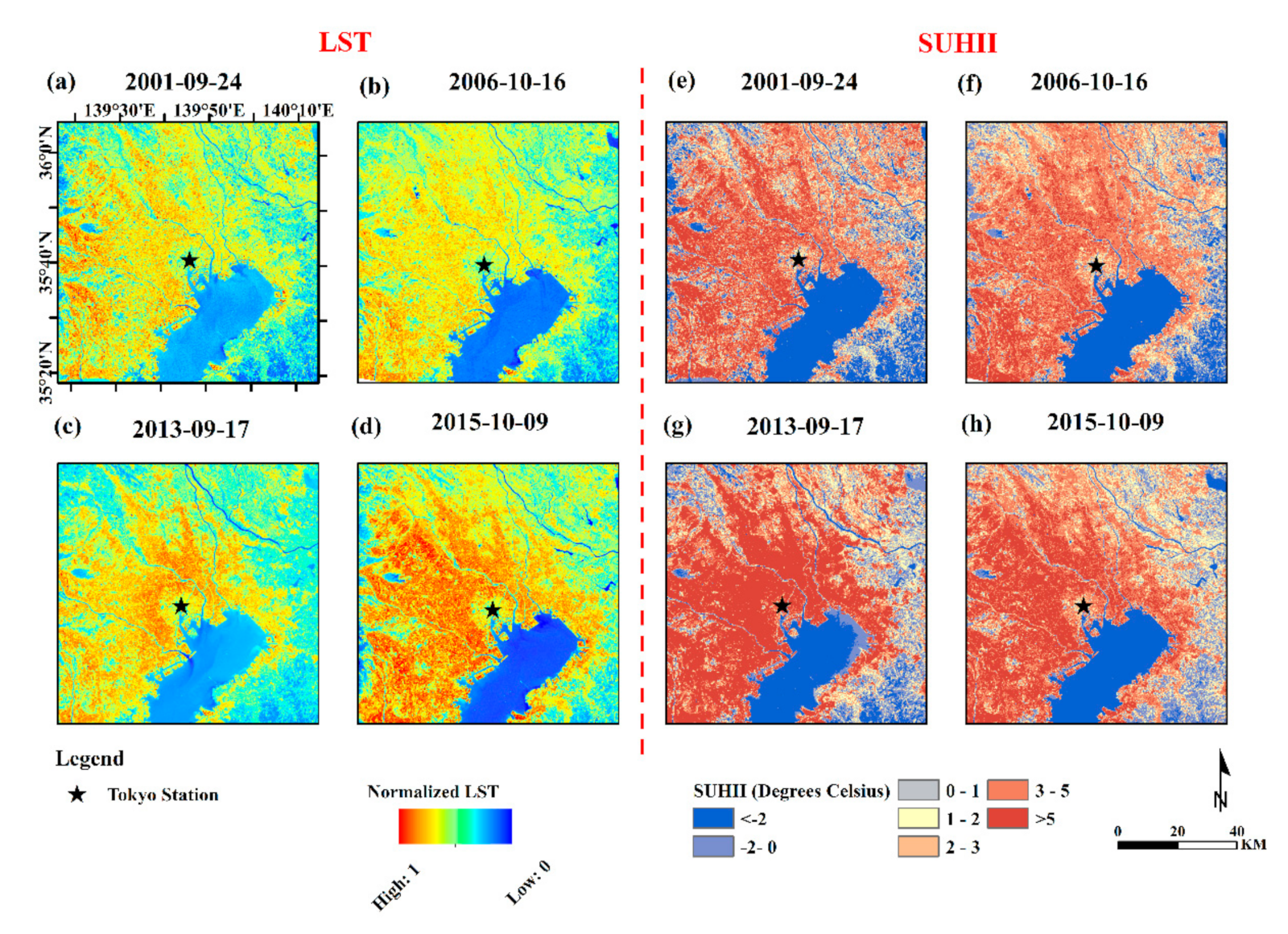
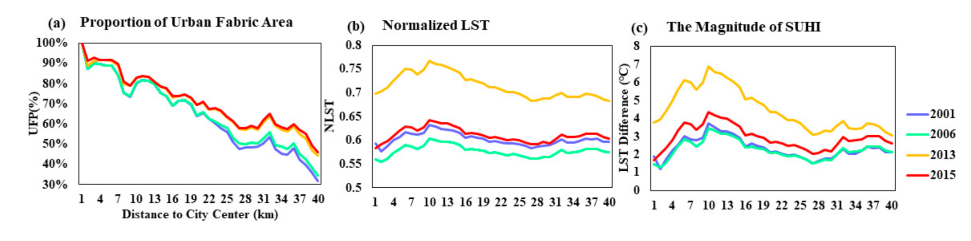
Intense human activities and land cover/use transformations alter the thermal properties of the urban land surface, which further causes the thermal imbalance of the urban system [11,50]. Figure 4 illustrates the spatiotemporal layout of the urban thermal environment across the TMA between 2001 and 2015. Figure 5 plots the curves for UFP, normalized LST (NLST), and SUHI variations based on urban–rural profiling. The spatial arrangement of UF in TMA between 2001 and 2015 exhibited typical urban–rural gradient distribution. The proportion of urbanized area gradually decreased from downtown to suburban areas. Spatially, radiating patterns of the thermal environment appeared in which the heat diffused from the highly urbanized inner-city area with high LST clustering outward to urban fringe areas and outskirts with low LST clustering. However, the peak value of LST was not located in the urban center despite the overall LST tendency of following the urban–rural temperature gradient pattern. We found that the values of NLST in 2001, 2006, 2013, and 2015 were similar. The curve of NLST arose from the origin (urban center) to the 10 km zone. In locations 10 km away from downtown, it climbed to the temperature peak and then gradually declined. The occurrence of NLST valleys and peaks was closely bound up with the accumulation of continuous urban areas. Accordingly, land cover/use exerted a considerable influence on the SUHI effect.
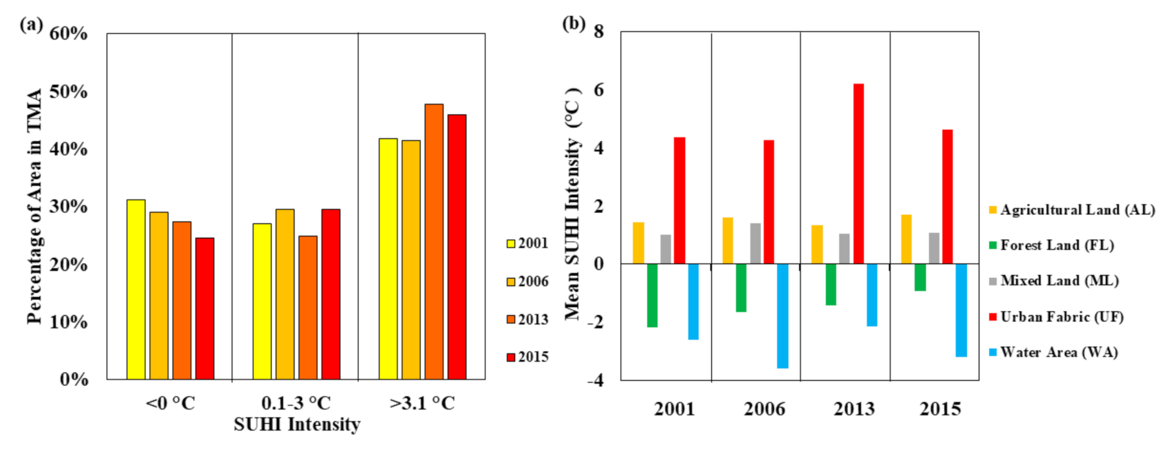
Figure 6a displays the percentage of area in TMA that experienced different SUHI effect levels from 2001 to 2015. The SUHI effect was more intense in 2013 than in 2001, 2006, and 2015. As shown in Figure 4 and Figure 6, the areas in TMA that experienced negative LST differences (<0 °C) continuously decreased from 31.18% in 2001 to 24.52% in 2015. The proportions of the area with 0.1–3 °C of LST difference were estimated at 27.03%, 29.58%, 24.83%, and 29.5% in 2001, 2006, 2013, and 2015, respectively. In 2001, the area with higher SUHII (>3.1 °C) occupied 41.78% of the whole region. This ratio was slightly reduced to 41.42% in 2006, increased to 47.81% in 2013, and then was 46% in 2015. The region with positive LST difference mainly pertained to UF. Moreover, the type of UF category always presented the maximum value of mean SUHII in TMA. The mean SUHII values for different kinds of land cover/use are shown in Figure 6b. As expected, positive thermal anomalies were observed in AL, ML, and UF, and negative thermal anomalies in FL and WL. The negative values indicate that urban greenery and water bodies have an unequivocal impact on the cooling effect. The influence of urban cooling gradually slowed down between 2001 and 2015, evidenced by the lower mean SUHII values. The highest and lowest cooling effect was detected in FL in 2001 (−2.18 °C) and 2015 (−0.92 °C).
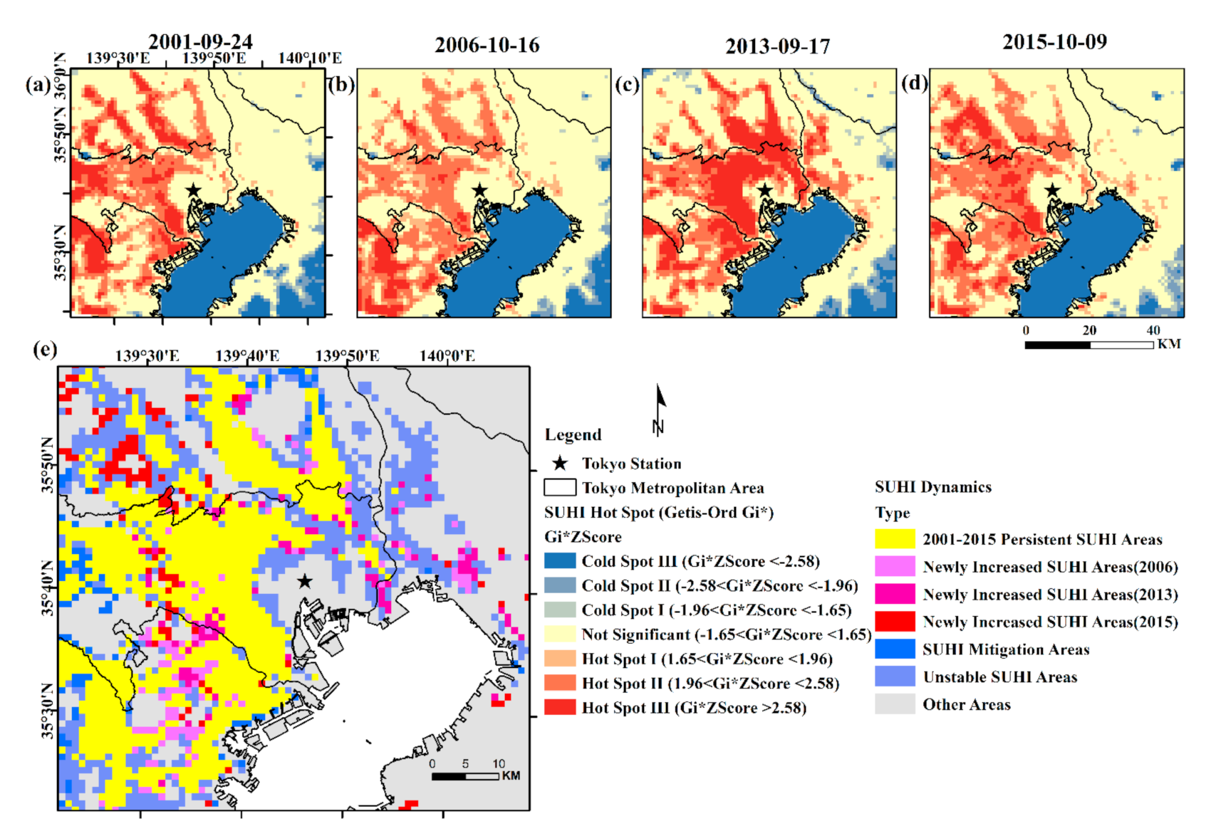
3.2. Interconnections of SUHII with Urban Development
This study examined SUHII hot/cold spots with statistical significance based on Getis-Ord local statistics, interpolated using the ordinary kriging method for visualization. Figure 7 shows the spatial locations of SUHII hot/cold spots and their variations. The hot spots were spatially distributed with a polycentric structure since 2001 (Figure 7a–d). The overall pattern of SUHI hot/cold spots maintained a relatively stable situation during the 15-year span. The MI values fluctuated and were estimated to be 0.88 in 2001, 0.90 in 2006, 0.89 in 2013, and 0.91 in 2015. SUHII in TMA displayed high spatial dependency. This implies that the thermal environment is homogeneous, and the spatiotemporal pattern of the SUHI effect exhibits the characteristics and tendency of convergence and aggregation.
From 2001 to 2015, SUHII hot spots I–III mainly emerged in the western part of TMA, between 10 km and 30 km from the urban core, and densely aggregated near low-rise residential buildings (Figure 7). The amount and extent of hot spot III in 2013 significantly increased compared to other years and those of hot spot II correspondingly decreased. The cold spot areas in TMA between 2001 and 2015 primarily occurred in areas with dense vegetation and water bodies, for example, Tokyo Bay, at the southeast edge of the study area. This finding suggests that abundant green space (forest, etc.) and large proportional water bodies would contribute to alleviating SUHI.
We combined the SUHII spatiotemporal aggregation patterns to yield the dynamics and variations of the thermal environment from 2001 to 2015, as shown in Figure 7e. The areas in TMA where strong SUHI effects occurred persistently between 2001 and 2015 occupied 19.69% of the whole research region. The newly increased SUHI areas in 2006, 2013, and 2015 were 115 km2, 98 km2, and 131 km2, respectively. The area that offset the thermal effect from 2001 to 2015 was estimated at 152 km2. In total, approximately 12.92% of the study region emerged as unstable as the result of SUHI between 2001 and 2015.
The centroids of SUHI hot spots at different periods were calculated to depict the different evolutionary tracks of TMA’s thermal environment over time. The centroids of UF on the whole regional scale from 2001 to 2015 were also measured. The centroids of UF were located at the area of 139.67–139.69°E, 35.69–35.71°N over the 15-year period. From 2001 to 2006, the UF centroid moved 537 m in the northern direction from the west. From 2006 to 2013, the movement tended toward the northeast over a distance of 1800 m. The centroid moved 466 m in the northeast direction from 2013 to 2015. This indicates that the leading orientation of urban expansion during 2001–2006 and 2006–2015 was northwest and northeast, respectively. The movement of SUHI centroids in TMA was distinguished from that of UF centroids due to the compound effect of multiple driving factors. However, the centroids of SUHI hot spots between 2001 and 2015 were all situated southwest of the UF centroids (continuous low/middle-rise residential quarters, west Tokyo). The centroid of SUHI hot spots moved southeast over a distance of 4636 m from 2001 to 2006. During 2006–2013, it shifted toward the northeast, moving about 8711 m. It then returned to the southwest, moving 6523 m between 2013 and 2015.
The different levels of SUHII-weighted SDEs in 2001, 2006, 2013, and 2015 were applied to reflect the spatiotemporal orientation, evolution, and trend of the urban thermal environment in TMA at the different phases, as shown in Figure 8. The specific parameters of SDEs are provided in Table A1 of Appendix A. The SDE analysis suggests that the spatial distribution of SUHI hot spots had apparent orientational effects over the whole research period.
3.3. Spatial Relationships of SUHII and Land Cover/Use
The VIF values of auxiliary variables are estimated at a threshold of less than 7.5 (Table 4), proving no multicollinearity among auxiliary variables. Ultimately, the SUHI formation in TMA was evaluated and modeled based on the GWR model by the explanatory variables of the CONTAG, elevation, population, UFP, and FP models. The result and diagnostic parameters are outlined in Table 5. The validity of global OLS and local GWR models was judged by adjusted R2, AICc, and MI of the standardized residual value (StdResid). For each research period, the global OLS model assessed the statistically significant relationship between SUHII and all determinants (joint F and Wald statistic ρ < 2.2 × 10⁻¹⁶). In TMA, the overall adjusted goodness-of-fit of the global OLS model was 0.65 (2001), 0.62 (2006), 0.84 (2013), and 0.72 (2015). The time sequence OLS model showed the same tendency in the four research stages. Among all determinants, the coefficients of CONTAG, population, and UFP were positively correlated and elevation and FP were negatively related to SUHII. The estimated coefficients in the OLS model indicate that the increments of CONTAG, population, and proportion of urban artificial coverage in TMA can facilitate the intensification of SUHI. In contrast, terrain and greenbelts can restrict and alleviate SUHI.
The modified coefficient of determination (R2) values for GWR models were all more than 0.9 (0.9082 in 2001, 0.9083 in 2006, 0.9322 in 2013, and 0.9132 in 2015). Compared to the OLS model, the MI of StdResid in the GWR model more closely approaches zero, indicating that the GWR model can provide better specifications of the spatial relationship between SUHII and its influencing variables than the conventional OLS model. The estimated F-values of GWR improvement by ANOVA also mirror a significant boost in simulating SUHII with the local GWR model. On account of spatially sensitive geographical variables, the GWR model enables the model parameters to spatially vary at a local scale, showing that corresponding spatial determinants have a non-stationary spatial effect on the SUHI phenomenon.
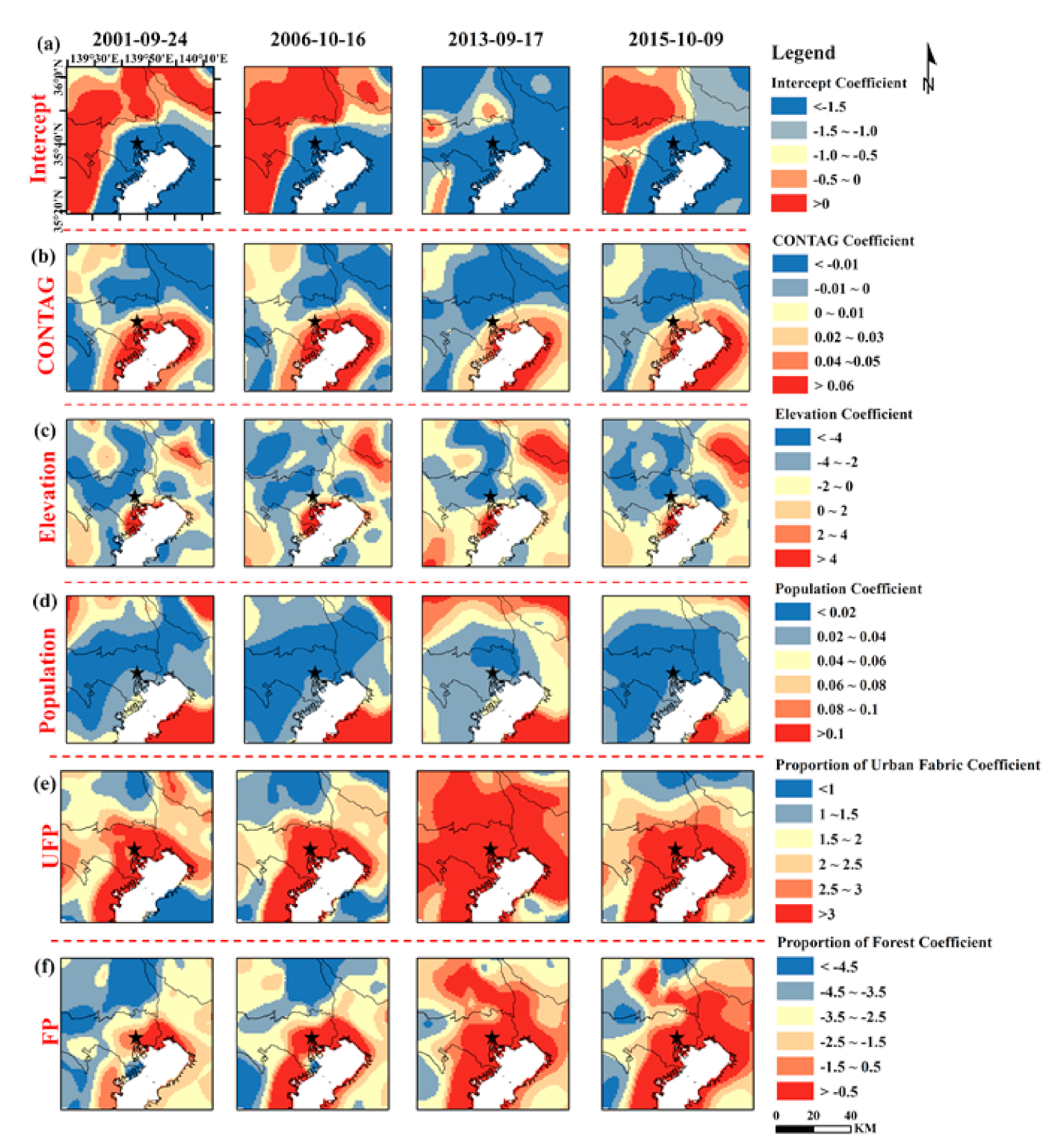
The localized spatial interconnection and differentiation between SUHII and underlying biophysical determinants in TMA from 2001 to 2015 are shown in Figure 9. The spatial variance of local estimates in 2013 was more distinct compared to other years. There were certain similarities in the spatial patterns of local coefficients in 2001, 2006, and 2015. A mix of positive and negative relationships between SUHI and CONTAG, varying over space, was identified. The spatial variance of CONTAG local coefficients from 2001 to 2015 primarily occurred in suburban settlements. In 2006 and 2013, elevation had an insignificant influence (ρ > 0.05) on the SUHI effect in TMA. Both positive and negative associations between SUHI and elevation were observed at a local scale from 2001 to 2015. Negative associations appeared in most areas, whereas positive relations were recognized in only some locations, such as Tokyo Bay shoreline and Ibaraki’s bare land areas. Human activities are centered in the urban–suburban area, and the variations of local relationships between SUHI and population between 2001 and 2015 were mainly seen in the urban/IS area. The mean coefficients of the population from 2001 to 2015 are 0.034 (2001), 0.026 (2006), 0.046 (2013), and 0.025 (2015).
The UFP has a significant positive effect on SUHII regardless of scale. We observed that the influence of UFP was more prevalent than that of other explanatory variables. The positive relationship constantly dominated the research region in terms of the UFP explanatory variable. However, the spatial relationship between SUHI and UFP was more intense in 2013 than in other years in which the area with higher coefficients (>2.5) significantly expanded. In the UF area from 2001 to 2015, the value of the mean UFP coefficient drastically increased from 2.33 to 4.11. However, the value peaked in 2013 and then dropped to 3.15 in 2015. Overall, the proportion of forest negatively correlated with SUHII between 2001 and 2015. The localized spatial relationship between SUHI and FP was noticeably diminished since 2001. The areas with high negative association had shrunk. In forest land, the values of mean FP coefficients varied in the range of −3.09 to −2.23. The peak of FP influence was in 2001, and the valley was in 2013.
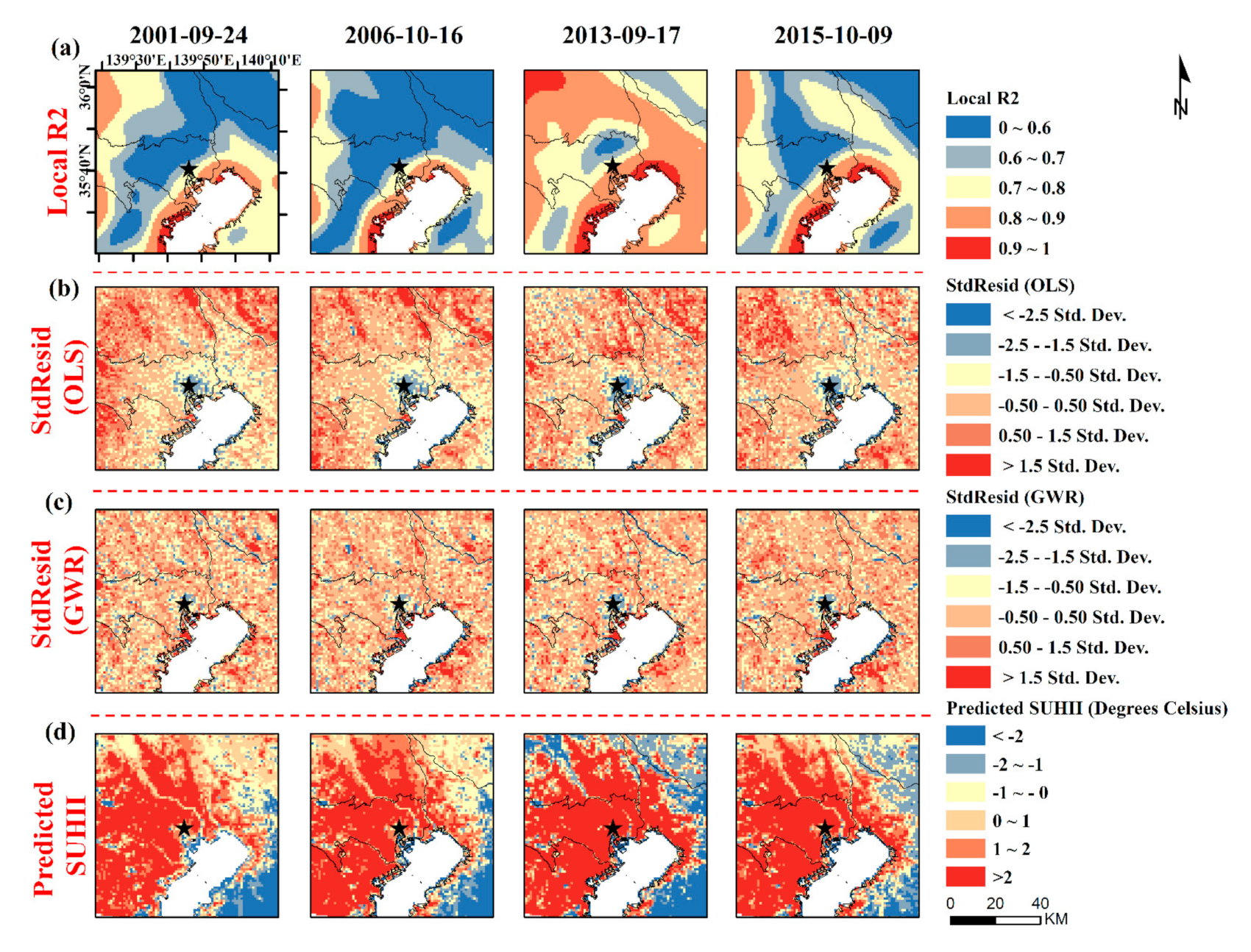
Interpreting the spatial relationship between SUHI magnitude in TMA and relevant exploratory variables using the GWR model, we can determine that there were many differences and linkages over time. The spatiotemporal variations of local R2 (Figure 10) mirror the spatial heterogeneity between SUHI and its exploratory variables over time. High values of local goodness-of-fit are measured in the region along the Tokyo Bay shoreline, while low values are concentrated in densely built-up areas or areas with IS coverage, such as downtown urban settlements. In addition, forces driving the formation of thermal differentiation in TMA were not static but varied from time to time as the urban environment and developments evolved. The spatially clustered distribution of StdResid derived from OLS and GWR models was identified (Figure 10) and verified by the MI index. The spatial aggregation patterns of StdResid in the conventional OLS model are more pronounced and discernable than in the local GWR model. The performance of fit between predicted and observed SUHII exceeds 86%. This indicates that SUHI formation in TMA during 2001–2015 can be simulated and investigated by these five auxiliary variables.
4. Discussion
4.1. Land Use Policies and SUHI Magnitude
We clarified the spatial and temporal disparities and variations in the SUHI pattern of TMA between 2001 and 2015. The analysis showed that certain biophysical (proportion of urban fabric, forest ratio, etc.) and social (population) characteristics of TMA’s urban environment favored the SUHI phenomenon. Spatial differentiation of SUHI formation and configuration by local non-stationarity GWR modeling has profound implications for urban comfort and sustainability in TMA.
Manley [84,85] proposed the term UHI and elaborated on the impacts of urban development processes on London’s climate system under the hypothesis of well-defined utilization of urban land. Numerous studies exemplified the relationship between urban land utilization, urban forms, and thermal anomalies [10,31]. As embodied in the previous studies, urban land utilization should be a dominant driving force [8,31,86]. Thus, relevant policies and plans are significantly bound up with SUHI formation and configuration. In the previous analysis, urban thermal gradients between UF and non-UF categories in TMA were examined by a joint analysis of ESA-CCI land cover/use products and Landsat-retrieved LST maps. Different from the results of classically defined SUHI investigations, the effects of SUHI in Tokyo were intensively clustered in residential and redevelopment areas, rather than in the central business district (CBD) (Figure 5). Hirano et al. [87] and Tsunematsu et al. [46,47] assessed the impact of UHI on Tokyo from the perspective of urban energy. They demonstrated that the high-density residential areas presented a severe heat energy agglomeration phenomenon, in agreement with our results. As in TMA, in several Asian megacities (e.g., Hong Kong, Guangzhou, Shanghai, Singapore) [43,86,88,89,90,91], the maximum SUHI magnitude was not detected in downtown or central commercial areas in recent years. The peak of diurnal thermal anomalies between urban and rural areas frequently emerged in high-density residential or industrial regions of these megacities. To cope with the urban thermal crisis, it is urgent to manage the thermal cores in the urban area of TMA.
The specific policy areas of development planning in TMA were designated for the upgrading and coordinating of regional development based on the National Capital Region Development Plan (https://www.toshiseibi.metro.tokyo.lg.jp/eng/) [92], as shown in Figure 11a. The official planning policies for the development of TMA resulted in a gradient urban–suburban–rural pattern in terms of urban infrastructure and settlement distribution. There are various types of urban land utilization in the built-up areas (BAs), specifically the TMA city proper, oriented for maintaining and improving the urban functions of TMA for socioeconomic activities, industrial manufacturing practices, and modern residential quarters. The mean SUHII for the BA of TMA increased from 3.97 °C in 2001 to 4.78 °C in 2015, and the peak value was 6.91 °C in 2013. In the BA of Tokyo, regions with large-scale residential quarters experienced severe SUHI impact between 2001 and 2015, involving Shinagawa, Ota, Setagaya, Suginami, Nakano, etc. Conversely, the degree of SUHI was not intense or strong in Tokyo’s downtown, including Chuo, Shibuya, Shinjuku, Koto, Chiyoda, etc.
It is worth noting that the heat island magnitude of compact high-rise/middle-rise residential areas was less than that of low-rise areas in TMA (Figure 11b). Solar radiance was partially obstructed by tall buildings, even skyscrapers, which was related to the loss of surface temperature. This phenomenon implies that urban morphology and geometry affect the urban thermal field. In addition, the investment in sustainable infrastructure and green-landscaped buildings has also contributed to relieving the high temperature of downtown TMA [27,93]. Analogously, Tsunematsu et al. [47] described the responses of different urban surfaces to thermal infrared (TIR) energy in downtown Tokyo at 2 m spatial resolution, confirming that the magnitude of heat islands in areas with commercial/office utilization was lower than in areas with compact residential buildings. Moreover, the intense SUHI effect did not occur frequently in the coastal regions of TMA. This phenomenon was difficult to explain using the spatial pattern of land cover/use and/or population shifts. In reality, the regional pattern and magnitude of SUHI in TMA probably varied due to the effects of land–sea breezes. That was confirmed by a couple of studies [48,94,95,96]. TMA is situated at the border between land and ocean, in which the thermal balance mechanism is highly climate-sensitive and unavoidably influenced by the land–sea breeze system.
Based on Figure 7 and Figure 8, we found that the effect of SUHI in 2006 was relieved compared to 2001, and the magnitude in 2015 was less than in 2013. The centroid trajectories of thermal island cores in TMA were different from those of urban development. The inconsistency of change patterns of SUHI and the centroid trajectories of the UF areas in TMA between 2001 and 2015 might have resulted from the influence of atmospheric conditions, especially wind direction. Meteorological conditions probably substantially affect the accuracy of profiling the thermal environment [48]. According to the diurnal (09:00–18:00, JST) observation data provided by JMA, the local prevailing wind direction in 2001 (9/24), 2006 (10/16), and 2013 (9/17) was from the north-northwest, whereas in 2015 (10/9), it was from the south. Consequently, this impacted and biased the movements of SUHI barycenters in TMA.
Green spaces and water bodies have a definitive role in delivering cooling effects. Lemus-Canovas et al. [95] reported that the temperature of continuous urban fabric areas in the Barcelona Metropolitan Area was detected up to 2.5 °C higher than the green urban areas. In the context of Bangkok, Jakarta, and Manila, urban green spaces registered temperatures approximately 3 °C lower than impervious surface areas [33]. The negative daytime thermal intensity in suburban green zone preservation areas (SGZPAs) occurred between 2001 and 2015 due to the presence of urban greenery and open green landscapes. Large bodies of water (e.g., Tokyo Bay) have a notable influence on TMA’s thermal environment as well, evidenced by their massive contribution to cold spots. Within the complicated urban system in TMA, such areas play a crucial role in balancing the urban surface energy system, fostering urban comfort with well-laid-out green spaces and water areas, in agreement with our results. Similar green areas and water spaces have also been developed in other megacities (e.g., Barcelona, Bangkok, Seoul, Hong Kong, etc.) [86,95,96,97,98].
Based on the results of spatial regression modeling, we confirmed that compound effects from multiple driving factors influenced SUHI magnitude in TMA. Observing the spatiotemporal variations of model residuals, we noticed that overprediction of SUHI magnitude was mostly generated in the agricultural and mixed lands of Saitama, Ibaraki, and Chiba. In contrast, underprediction of thermal anomalies consistently occurred in TMA’s downtown. This indicates that investigations of the SUHI effect in the downtown area should consider more potential driving factors due to its complexity. The ongoing vertical and horizontal urbanization of TMA [97,98] cannot be neglected in coordinating the urban environment. Thus, we plan to collect more parameters of TMA’s urban environment (e.g., urban volume, sky view factor) to study and model the geographic processes of the complicated SUHI phenomenon with more advanced models and algorithms.
In the future, we expect to explore the interannual, seasonal, and diurnal thermal trends of TMA, fusing multisensor and multitemporal data. For example, satellite TIR images should be combined with synchronous data from microwave radiometer measurements and in situ observations to yield more reliable resultants. More detailed features of TMA’s urban biophysical environment using local climate zones or unmanned aerial vehicles (UAVs) should be considered in further investigations.
4.2. Toward a Livable Urban Environment
In this study, we explored the geographic mechanism and process between land use/cover and the magnitude of the urban thermal effect in the urban aggregation of TMA based on spatial statistical analysis. The mechanism of SUHI formation in TMA is extremely complicated, influenced by more than the land cover/use composition and configuration. Nevertheless, we can partially study and interpret the confounding effects of SUHI using combinations of different variables. The detailed differentiation of whether the spatial mechanisms of heat islands in TMA were influenced by underlying physical factors was based on both global and local modeling. This can provide sufficient evidence for ameliorating the intensive thermal effect. Spatially, the geographic process of the SUHI effect in TMA manifested high heterogeneity according to the non-stationarity GWR modeling framework. Since the values of SUHII significantly vary over space, the thermal impact on TMA is context-sensitive and can be locally assessed based on spatial determinants from neighborhoods. That is mirrored in need for localized landscape planning and site-specific policy design to minimize the SUHI phenomenon. There are favorable evidence and references regarding the use of localized policy design to control the formation of SUHI across diverse cities around the world, such as Brisbane [41], Hangzhou [42], Las Vegas [77], Texas [76], and Ljutomer [74].
Furthermore, this study confirmed that SUHI barycenters and hotspot areas were detected in compact low-rise residential quarters through spatial aggregation analysis and spatial centroid movement. Tokyo is dominated by a large ratio of impervious surfaces and compact buildings. Due to scarce land assets and fierce competition for land resource development, it is hard to put into effect urban greening policies in severe thermal spots. In addition, it has been acknowledged that in Tokyo Metropolis there was a deteriorating trend in urban greenery; the area of emerging green coverage varied from 31,535 m2 in 2001 to 58,227 m2 in 2006, then went down to 33,234 m2 in 2013 and 26,444 m2 in 2015 (data from Program of Creating Urban Green Spaces, Bureau of Environment, TMG) [17,20]. Impervious artificial landscapes and green spaces are dominant components in the urban setting. Thus, sustainable infrastructure and green retrofit, as the most appropriate and practical measures, should be increased to mitigate clustered SUHI.
We expect that local authorities in TMA could reinforce urban climate responses and management by adopting a group of mitigating measures, including expanding urban forests along the highways and in urban parks; cultivating and maintaining green corridors surrounding rivers, lakes, or ponds; and promoting small patches of green landscapes neighboring compact residences.
Japanese coastal megacities, such as Sendai and Fukuoka, have also built livable urban environments by adopting urban afforestation strategies [25,99]. In addition, the construction and enhancement of urban ventilation corridors have become important in UHI alleviation as well. The city temperature in dense IS areas can be decreased by enhancing the ventilation cooling effects and controlling the number of green spaces and buildings in SUHI hot spots. Asian coastal megacities such as Hong Kong, Shanghai, and Singapore have also implemented similar countermeasures for SUHI abatement [86,100].
5. Conclusions
In this study, we targeted the TMA as a crucial case study to evaluate the spatiotemporal response of land cover/use on surface temperature. This study’s distinctiveness lies chiefly in its consideration of neighboring plans and localized landscape design on surface temperature in the metropolitan area of Tokyo over time and space based on a multitude of driving forces. In addition, the occurrence of SUHI depends on the compound effects of multiple drivers. Forces with different thermal impact magnitudes are not static but spatiotemporally varied, relying on the local geographical setting and urban development process. Hence, this study highlights the following:
(1) The uniqueness and complexity of the SUHI effect in TMA: TMA’s thermal environment profile showed an overall upward trend of LST and SUHII between 2001 and 2015. Based on the SUHI aggregation pattern, TMA was recognized as an area with multiple thermal cores. Dense thermal islands occurred in the compact residential quarters and redevelopment/renovation areas, rather than in downtown (CBD). The distribution of tall buildings shielding solar radiation and the contributions of water bodies and sea breezes might be two reasons for this phenomenon;
(2) The identification of spatiotemporal interconnections between land cover/use and thermal environment based on global and local regression modeling: Land cover/use composition, landscape configuration, terrain, population density, and afforestation ratios have altered the balance of the urban thermal-energy system in TMA. Synergistic use of OLS (global) and GWR (local) models could effectively detect potential influencing factors and accordingly propose entire/partial SUHI mitigation strategies.
Overall, in order to create a sustainable and livable urban environment, local authorities in TMA should pay attention to offsetting the magnitude of SUHI cluster spots and carefully controlling the formation of SUHIs in non-significant areas. We suggest that urban afforestation be fine-tuned based on partitioned or location-specific landscape design by incorporating the green measures adopted by local communities and the private sector.
Author Contributions
Conceptualization, F.L., H.H., and Y.M.; methodology, F.L.; software, F.L.; formal analysis, F.L.; investigation, F.L.; resources, F.L.; data curation, F.L.; writing—original draft preparation, F.L.; writing—review and editing, H.H. and Y.M.; visualization, F.L.; supervision, Y.M.; project administration, Y.M.; funding acquisition, H.H. and Y.M. All authors have read and agreed to the published version of the manuscript.
Funding
This study was partly supported by JSPS grant 18H00763 (2018-20, representative: Yuji Murayama), Japan, and the Natural Science Foundation of Zhejiang Province (grant number LQ20D010008, representative: Hao Hou), China.
Data Availability Statement
The data that support the findings of this study are available on reasonable request from the corresponding author.
Acknowledgments
The authors highly appreciate the editors and anonymous reviewers for their valuable and constructive comments and suggestions to improve the manuscript.
Conflicts of Interest
The authors declare no conflict of interest.
Appendix A

Table A1.
SDE parameters of SUHI hot spots from 2001 to 2015.
| Serial no. (year) | Centroid_X (Longitude °) | Centroid_Y (Latitude °) | Long Axis (m) | Short Axis (m) | Long Axis/Short Axis | Rotation (°) |
|---|---|---|---|---|---|---|
| 2001 | 139.54 | 35.68 | 29,227.03 | 18,516.53 | 1.58 | 23.73 |
| 2006 | 139.55 | 35.64 | 30,823.80 | 16,857.33 | 1.83 | 24.67 |
| 2013 | 139.64 | 35.68 | 28,311.34 | 19,289.65 | 1.47 | 43.86 |
| 2015 | 139.57 | 35.67 | 27,584.21 | 20,305.18 | 1.36 | 16.44 |
References
- World Climate Research Programme (WCRP). Global Research and Action Agenda on Cities and Climate Change Science-Full Version; Prieur-Richard, A.H., Walsh, M.B., Craig, M.L., Melamed, M., Colbert, M., Pathak, S., Connors, X., Bai, A., Barau, H., Bulkeley, H., et al., Eds.; WCRP Publication No.13, 2019; Available online: https://www.wcrp-climate.org/WCRP-publications/2019/GRAA-Cities-and-Climate-Change-Science-Full.pdf (accessed on 15 December 2020).
- United Nations (UN). United Nations Framework Convention on Climate Change. Available online: https://unfccc.int/resource/docs/convkp/conveng.pdf (accessed on 15 December 2020).
- Intergovernmental Panel on Climate Change (IPCC). Climate Change 2014: Mitigation of Climate Change; Edenhofer, O., Pichs-Madruga, Y.R., Sokona, E., Farahani, S., Kadner, K., Seyboth, A., Adler, I., Baum, S., Brunner, P., Eickemeier, B., et al., Eds.; Cambridge University Press: Cambridge, UK, 2014. [Google Scholar]
- Castán Broto, V.; Bulkeley, H. A survey of urban climate change experiments in 100 cities. Glob. Environ. Chang. 2013, 23, 92–102. [Google Scholar] [CrossRef] [PubMed] [Green Version]
- Gago, E.J.; Roldan, J.; Pacheco-Torres, R.; Ordóñez, J. The city and urban heat islands: A review of strategies to mitigate adverse effects. Renew. Sustain. Energy Rev. 2013, 25, 749–758. [Google Scholar] [CrossRef]
- Rosenzweig, C.; Solecki, W.D.; Romero-Lankao, P.; Mehrotra, S.; Dhakal, S.; Ibrahim, S.A. Climate Change and Cities: First Assessment Report of the Urban Climate Change Research Network; Cambridge University Press: Cambridge, UK, 2011. [Google Scholar]
- Voogt, J.A.; Oke, T.R. Thermal remote sensing of urban climates. Remote Sens. Environ. 2003, 86, 370–384. [Google Scholar] [CrossRef]
- Weng, Q. Thermal infrared remote sensing for urban climate and environmental studies: Methods, applications, and trends. ISPRS J. Photogramm. Remote Sens. 2009, 64, 335–344. [Google Scholar] [CrossRef]
- Oke, T.R. The energetic basis of the urban heat island. Q. J. R. Meteorol. Soc. 1982, 108, 1–24. [Google Scholar] [CrossRef]
- Deilami, K.; Kamruzzaman, M.; Liu, Y. Urban heat island effect: A systematic review of spatio-temporal factors, data, methods, and mitigation measures. Int. J. Appl. Earth Obs. Geoinf. 2018, 67, 30–42. [Google Scholar] [CrossRef]
- Ahmed Memon, R.; Leung, D.Y.; Chunho, L. A review on the generation, determination and mitigation of urban heat island. J. Environ. Sci. 2008, 20, 120–128. [Google Scholar]
- Nuruzzaman, M. Urban heat island: Causes, effects and mitigation measures—A review. Int. J. Environ. Monit. Anal. 2015, 3, 67. [Google Scholar] [CrossRef] [Green Version]
- United Nations, Department of Economic and Social Affairs, Population Division, (UN DESA). World Population Prospects: The 2015 Revision; UN DESA: New York, NY, USA, 2015. [Google Scholar]
- United Nations, Department of Economic and Social Affairs, Population Division, (UN DESA). World Urbanization Prospects: The 2018 Revision; UN DESA: New York, NY, USA, 2018. [Google Scholar]
- Gerden, T. The adoption of the Kyoto protocol of the United Nations framework convention on climate change. Contrib. Contemp. Hist. 2018, 58. [Google Scholar] [CrossRef]
- Statistic Bureau of Japan. Statistical Handbook of Japan. Available online: https://www.stat.go.jp/english/data/handbook/index.html (accessed on 15 December 2020).
- The Bureau of Environment, Tokyo Metropolitan Government (TMG). Creating a Sustainable City-Tokyo’s Environmental Policy. Available online: https://www.metro.tokyo.lg.jp/english/about/environmental_policy/index.html (accessed on 15 December 2020).
- Centre for Regional Research, Hosei University. Report on Local Climate Change Adaptation in Japan. Available online: https://si-cat.ws.hosei.ac.jp/en/paper2016en_web.pdf (accessed on 15 December 2020).
- Association of International Research Initiatives for Environmental Studies (AIRIES). Perspectives on climate change research in Japan after the Paris Agreement: International negotiations, technologies and countermeasures, plus adaptation. Glob. Environ. Res. 2017, 21, 1–64. [Google Scholar]
- Statistics Division at Bureau of General Affairs, TMG. Tokyo Statistical Yearbook. Available online: https://www.toukei.metro.tokyo.lg.jp/tnenkan/tn-eindex.html (accessed on 15 December 2020).
- Statistic Bureau of Japan. Japan Statistical Yearbook. Available online: https://www.stat.go.jp/english/data/nenkan/ (accessed on 15 December 2020).
- The Bureau of Environment, TMG. Environmental Outlook Tokyo. Available online: https://www.kankyo.metro.tokyo.lg.jp/en/about_us/videos_documents/documents_1.files/kankyo4774.pdf (accessed on 15 December 2020).
- The Bureau of Environment, TMG. Urban Heat Island. Available online: https://www.kankyo.metro.tokyo.lg.jp/en/climate/heat_island.html (accessed on 15 December 2020).
- Case, M.; Tidwell, A. Nippon Changes: Climate Impacts Threatening Japan Today and Tomorrow; World Wildlife Fund (WWF) International: Gland, Switzerland, 2008. [Google Scholar]
- Japan Meteorological Agency (JMA). Climate Change Monitoring Report. Available online: https://www.jma.go.jp/jma/en/NMHS/indexe_ccmr.html (accessed on 15 December 2020).
- Ministry of the Environment (MOE); Ministry of Education, Culture, Sports, Science and Technology (MEXT); Ministry of Agriculture, Forestry and Fisheries (MAFF); Ministry of Land, Infrastructure, Transport and Tourism (MLIT); Japan Meteorological Agency (JMA). Climate Change and Its Impacts in Japan. Synthesis Report on Observations, Projections, and Impact Assessments of Climate Change Climate. 2018. Available online: https://www.env.go.jp/earth/tekiou/pamph2018_full_Eng.pdf (accessed on 15 December 2020).
- The Bureau of Environment, TMG. Guidelines for Heat Island Control Measures. Available online: https://www.kankyo.metro.tokyo.lg.jp/en/about_us/videos_documents/documents_1.files/heat_island.pdf (accessed on 15 December 2020).
- Ministry of the Environment (MOE), Japan. Annual Report on Environmental Statistics. Available online: https://www.env.go.jp/en/statistics/ (accessed on 15 December 2020).
- Inter-Ministry Coordination Committee to Mitigate Urban Heat Island. Outline of the Policy Framework to Reduce Urban Heat Island Effects. Available online: https://www.env.go.jp/en/air/heat/heatisland.pdf (accessed on 15 December 2020).
- Kusaka, H. Recent progress on urban climate study in Japan. Geogr. Rev. Jpn. 2019, 53, 1689–1699. [Google Scholar] [CrossRef] [Green Version]
- Zhou, D.; Xiao, J.; Bonafoni, S.; Berger, C.; Deilami, K.; Zhou, Y.; Frolking, S.; Yao, R.; Qiao, Z.; Sobrino, J.A. Satellite remote sensing of surface urban heat islands: Progress, challenges, and perspectives. Remote Sens. 2019, 11, 48. [Google Scholar] [CrossRef] [Green Version]
- Estoque, R.C.; Murayama, Y.; Myint, S.W. Effects of landscape composition and pattern on land surface temperature: An urban heat island study in the megacities of Southeast Asia. Sci. Total Environ. 2017, 577, 349–359. [Google Scholar] [CrossRef] [PubMed]
- Fan, C.; Myint, S.W.; Kaplan, S.; Middel, A.; Zheng, B.; Rahman, A.; Huang, H.P.; Brazel, A.; Blumberg, D.G. Understanding the impact of urbanization on surface urban heat Islands-A longitudinal analysis of the oasis effect in subtropical desert cities. Remote Sens. 2017, 9, 672. [Google Scholar] [CrossRef] [Green Version]
- Tayyebi, A.; Shafizadeh-Moghadam, H.; Tayyebi, A.H. Analyzing long-term spatio-temporal patterns of land surface temperature in response to rapid urbanization in the megacity of Tehran. Land Policy 2018, 71, 459–469. [Google Scholar] [CrossRef]
- Chen, W.; Zhang, Y.; Pengwang, C.; Gao, W. Evaluation of urbanization dynamics and its impacts on surface heat islands: A case study of Beijing, China. Remote Sens. 2017, 9, 453. [Google Scholar] [CrossRef] [Green Version]
- Keeratikasikorn, C.; Bonafoni, S. Urban heat island analysis over the land use zoning plan of Bangkok by means of Landsat 8 imagery. Remote Sens. 2018, 10, 440. [Google Scholar] [CrossRef]
- Simwanda, M.; Ranagalage, M.; Estoque, R.C.; Murayama, Y. Spatial analysis of surface urban heat islands in four rapidly growing African cities. Remote Sens. 2019, 11, 1645. [Google Scholar] [CrossRef] [Green Version]
- Dissanayake, D.; Morimoto, T.; Murayama, Y.; Ranagalage, M.; Handayani, H.H. Impact of urban surface characteristics and socio-economic variables on the spatial variation of land surface temperature in Lagos City, Nigeria. Sustainability 2018, 11, 25. [Google Scholar] [CrossRef] [Green Version]
- Dissanayake, D.M.S.L.B.; Morimoto, T.; Murayama, Y.; Ranagalage, M. Impact of landscape structure on the variation of land surface temperature in Sub-Saharan Region: A case study of Addis Ababa using Landsat data (1986–2016). Sustainability 2019, 11, 2257. [Google Scholar] [CrossRef] [Green Version]
- Hou, H.; Estoque, R.C. Detecting cooling effect of landscape from composition and configuration: An urban heat island study on Hangzhou. Urban For. Urban Green. 2020, 53. [Google Scholar] [CrossRef]
- Deilami, K.; Kamruzzaman, M.; Hayes, J.F. Correlation or causality between land cover patterns and the urban heat island effect? Evidence from Brisbane, Australia. Remote Sens. 2016, 8, 716. [Google Scholar] [CrossRef] [Green Version]
- Li, F.; Sun, W.; Yang, G.; Weng, Q. Investigating spatiotemporal patterns of surface urban heat islands in the Hangzhou Metropolitan Area, China, 2000. Remote Sens. 2019, 11, 1553. [Google Scholar] [CrossRef] [Green Version]
- Liu, F.; Zhang, X.; Murayama, Y.; Morimoto, T. Impacts of land cover/use on the urban thermal environment: A comparative study of 10 megacities in China. Remote Sens. 2020, 12, 307. [Google Scholar] [CrossRef] [Green Version]
- Wang, R.; Murayama, Y. Geo-simulation of land use/cover scenarios and impacts on land surface temperature in Sapporo, Japan. Sustain. Cities Soc. 2020, 63, 102432. [Google Scholar] [CrossRef]
- Wang, L.; Hou, H.; Weng, J. Ordinary least squares modelling of urban heat island intensity based on landscape composition and configuration: A comparative study among three megacities along the Yangtze River. Sustain. Cities Soc. 2020, 62, 102381. [Google Scholar] [CrossRef]
- Tsunematsu, N.; Yokoyama, H.; Honjo, T.; Ichihashi, A.; Ando, H.; Matsumoto, F.; Seto, Y.; Shigyo, N.; Games, P. Impacts of Urban Heat Island Mitigation Strategies on Surface Temperatures in Downtown Tokyo. In Proceedings of the 9th International Conference on Urban Climate Jointly with 12th Symposium on the Urban Environment, Toulouse, France, 20–24 July 2015; Available online: http://www.meteo.fr/icuc9/LongAbstracts/ccma7-2-1471106_a.pdf (accessed on 15 December 2020).
- Tsunematsu, N.; Yokoyama, H.; Honjo, T.; Ichihashi, A.; Ando, H.; Shigyo, N. Relationship between land use variations and spatiotemporal changes in amounts of thermal infrared energy emitted from urban surfaces in downtown Tokyo on hot summer days. Urban. Clim. 2016, 17, 67–79. [Google Scholar] [CrossRef]
- Zhou, X.; Okaze, T.; Ren, C.; Cai, M.; Ishida, Y.; Watanabe, H.; Mochida, A. Evaluation of urban heat islands using local climate zones and the influence of sea-land breeze. Sustain. Cities Soc. 2020, 55, 102060. [Google Scholar] [CrossRef]
- Mirzaei, P.A. Recent challenges in modeling of urban heat island. Sustain. Cities Soc. 2015, 19, 200–206. [Google Scholar] [CrossRef] [Green Version]
- Mohajerani, A.; Bakaric, J.; Jeffrey-Bailey, T. The urban heat island effect, its causes, and mitigation, with reference to the thermal properties of asphalt concrete. J. Environ. Manag. 2017, 197, 522–538. [Google Scholar] [CrossRef] [PubMed]
- European Space Agency (ESA). Land Cover CCI Product User Guide Version 2 Tech. Rep. 2017. Available online: maps.elie.ucl.ac.be/CCI/viewer/download/ESACCI-LC-Ph2-PUGv2_2.0.pdf (accessed on 15 December 2020).
- Lamarche, C.; Bontemps, S.; Verhegghen, A.; Radoux, J.; Vanbogaert, E.; Kalogirou, V.; Seifert, F.M.; Arino, O.; Defourny, P. Characterizing the Surface Dynamics for Land Cover Mapping: Current Achievements of the ESA CCI Land Cover. ESA Special Publication, 2013. Available online: https://ftp.space.dtu.dk/pub/Ioana/papers/s333_4lama.pdf (accessed on 15 December 2020).
- McGarigal, K.; Cushman, S.A.; Neel, M.C.; Ene, E. FRAGSTATS: Spatial Pattern Analysis Program for Categorical Maps. Available online: http://www.umass.edu/landeco/research/fragstats/fragstats.html (accessed on 15 December 2020).
- Liu, F.; Murayama, Y. Landsat evaluation of land cover composition and its impacts on urban thermal environment: A case study on the fast-growing Shanghai Metropolitan Area. Geoinfor Geostat Overv. 2018, 2. [Google Scholar] [CrossRef]
- Yu, X.; Guo, X.; Wu, Z. Land surface temperature retrieval from Landsat 8 TIRS-comparison between radiative transfer equation-based method, split window algorithm and single channel method. Remote Sens. 2014, 6, 9829–9852. [Google Scholar] [CrossRef] [Green Version]
- Sobrino, J.A.; Jiménez-Muñoz, J.C.; Paolini, L. Land surface temperature retrieval from Landsat TM 5. Remote Sens. Environ. 2004, 90, 434–440. [Google Scholar] [CrossRef]
- McCarville, D.; Buenemann, M.; Bleiweiss, M.; Barsi, J. Atmospheric correction of Landsat thermal infrared data: A calculator based on North American Regional Reanalysis (NARR) data. In Proceedings of the American Society for Photogrammetry and Remote Sensing Conference, Milwaukee, WI, USA, 1–5 May 2011; Volume 15. [Google Scholar]
- Barsi, A.J.; Barker, L.J.; Schott, R.J. An atmospheric Correction Parameter Calculator for a Single Thermal Band Earth-Sensing Instrument. In Proceedings of the 2003 IEEE International Geoscience and Remote Sensing Symposium, Toulouse, France, 21–25 July 2003; Volume 5, pp. 3014–3016. [Google Scholar]
- Barsi, J.A.; Schott, J.R.; Palluconi, F.D.; Hook, S.J. Validation of a web-based atmospheric correction tool for single thermal band instruments. Earth Obs. Syst. 2005, 5882, 58820E. [Google Scholar] [CrossRef]
- Weng, Q.; Lu, D. A sub-pixel analysis of urbanization effect on land surface temperature and its interplay with impervious surface and vegetation coverage in Indianapolis, United States. Int. J. Appl. Earth Obs. Geoinf. 2008, 10, 68–83. [Google Scholar] [CrossRef]
- Deilami, K.; Kamruzzaman, M. Modelling the urban heat island effect of smart growth policy scenarios in Brisbane. Land Policy 2017, 64, 38–55. [Google Scholar] [CrossRef]
- Tran, D.X.; Pla, F.; Latorre-Carmona, P.; Myint, S.W.; Caetano, M.; Kieu, H.V. Characterizing the relationship between land use land cover change and land surface temperature. ISPRS J. Photogramm. Remote Sens. 2017, 124, 119–132. [Google Scholar] [CrossRef] [Green Version]
- Getis, A.; Ord, J.K. The analysis of spatial association by use of distance statistics. Geogr. Anal. 1992, 24, 189–206. [Google Scholar] [CrossRef]
- Ord, J.K.; Getis, A. Local spatial autocorrelation statistics: Distributional issues and an application. Geogr. Anal. 1995, 27, 286–306. [Google Scholar] [CrossRef]
- Griffith, D.A. Towards a theory of spatial statistics. Geogr. Anal. 1980, 12, 325–339. [Google Scholar] [CrossRef]
- Griffith, D.A. Theory of Spatial Statistics. In Spatial Statistics and Models; Springer: Dordrecht, The Netherlands, 1984; pp. 3–15. [Google Scholar]
- Lefever, D.W. Measuring geographic concentration by means of the standard deviational ellipse. Am. J. Sociol. 1926, 32, 88–94. [Google Scholar] [CrossRef]
- Wang, B.; Shi, W.; Miao, Z. Confidence analysis of standard deviational ellipse and its extension into higher dimensional Euclidean space. PLoS ONE 2015, 10, e0118537. [Google Scholar] [CrossRef]
- Xu, J.; Zhao, Y.; Zhong, K.; Zhang, F.; Liu, X.; Sun, C. Measuring spatio-temporal dynamics of impervious surface in Guangzhou, China, from 1988 to 2015, using time-series Landsat imagery. Sci. Total Environ. 2018, 627, 264–281. [Google Scholar] [CrossRef]
- Johnson, D.P.; Wilson, J.S. The socio-spatial dynamics of extreme urban heat events: The case of heat-related deaths in Philadelphia. Appl. Geogr. 2009, 29, 419–434. [Google Scholar] [CrossRef]
- Szymanowski, M.; Kryza, M. Local regression models for spatial interpolation of urban heat island-an example from Wrocław, SW Poland. Appl. Clim. 2012, 108, 53–71. [Google Scholar] [CrossRef] [Green Version]
- Li, L.; Zha, Y.; Zhang, J. Spatially non-stationary effect of underlying driving factors on surface urban heat islands in global major cities. Int. J. Appl. Earth Obs. Geoinf. 2020, 90, 102131. [Google Scholar] [CrossRef]
- Noi, P.T.; Degener, J.; Kappas, M. Comparison of multiple linear regression, cubist regression, and random forest algorithms to estimate daily air surface temperature from dynamic combinations of MODIS LST data. Remote Sens. 2017, 9, 398. [Google Scholar] [CrossRef] [Green Version]
- Ivajnšič, D.; Kaligarič, M.; Žiberna, I. Geographically weighted regression of the urban heat island of a small city. Appl. Geogr. 2014, 53, 341–353. [Google Scholar] [CrossRef]
- Dutilleul, P.; Legendre, P. Spatial heterogeneity against heteroscedasticity: An ecological paradigm versus a statistical concept. Oikos 1993, 66, 152–171. [Google Scholar] [CrossRef]
- Zhao, C.; Jensen, J.; Weng, Q.; Weaver, R. A geographically weighted regression analysis of the underlying factors related to the surface urban heat island phenomenon. Remote Sens. 2018, 10, 1428. [Google Scholar] [CrossRef] [Green Version]
- Wang, Z.; Fan, C.; Zhao, Q.; Myint, S.W. A geographically weighted regression approach to understanding urbanization impacts on urban warming and cooling: A case study of Las Vegas. Remote Sens. 2020, 12, 222. [Google Scholar] [CrossRef] [Green Version]
- Yin, C.; Yuan, M.; Lu, Y.; Huang, Y.; Liu, Y. Effects of urban form on the urban heat island effect based on spatial regression model. Sci. Total Environ. 2018, 634, 696–704. [Google Scholar] [CrossRef]
- Tatem, A.J. WorldPop, open data for spatial demography. Sci. Data 2017, 4, 1–4. [Google Scholar] [CrossRef]
- Lloyd, C.T.; Sorichetta, A.; Tatem, A.J. High resolution global gridded data for use in population studies. Sci. Data 2017, 4, 1–17. [Google Scholar] [CrossRef] [Green Version]
- Stevens, F.R.; Gaughan, A.E.; Linard, C.; Tatem, A.J. Disaggregating census data for population mapping using random forests with remotely-sensed and ancillary data. PLoS ONE 2015, 10, e0107042. [Google Scholar] [CrossRef] [Green Version]
- Farr, T.G.; Rosen, P.A.; Caro, E.; Crippen, R.; Duren, R.; Hensley, S.; Kobrick, M.; Paller, M.; Rodriguez, E.; Roth, L.; et al. The shuttle radar topography mission. Rev. Geophys. 2007, 45, 1–33. [Google Scholar] [CrossRef] [Green Version]
- Luo, X.; Peng, Y. Scale effects of the relationships between urban heat islands and impact factors based on a geographically-weighted regression model. Remote Sens. 2016, 8, 760. [Google Scholar] [CrossRef] [Green Version]
- Manley, G. On the frequency of snowfall in Metropolitan England. Q. J. R. Meteorol. Soc. 1958, 84, 70–72. [Google Scholar] [CrossRef]
- De Peres, L.F.; de Lucena, A.J.; Rotunno Filho, O.C.; de França, J.R.A. The urban heat island in Rio de Janeiro, Brazil, in the last 30 years using remote sensing data. Int. J. Appl. Earth Obs. Geoinf. 2018, 64, 104–116. [Google Scholar] [CrossRef]
- Zhang, H.; Qi, Z.; Ye, X.; Cai, Y.; Ma, W.; Chen, M. Analysis of land use/land cover change, population shift, and their effects on spatiotemporal patterns of urban heat islands in metropolitan Shanghai, China. Appl. Geogr. 2013, 44, 121–133. [Google Scholar] [CrossRef]
- Hirano, Y.; Fujita, T. Evaluation of the impact of the urban heat island on residential and commercial energy consumption in Tokyo. Energy 2012, 37, 371–383. [Google Scholar] [CrossRef]
- Xiong, Y.; Huang, S.; Chen, F.; Ye, H.; Wang, C.; Zhu, C. The impacts of rapid urbanization on the thermal environment: A remote sensing study of Guangzhou, South China. Remote Sens. 2012, 4, 2033–2056. [Google Scholar] [CrossRef] [Green Version]
- Kardinal Jusuf, S.; Wong, N.H.; Hagen, E.; Anggoro, R.; Hong, Y. The influence of land use on the urban heat island in Singapore. Habitat Int. 2007, 31, 232–242. [Google Scholar] [CrossRef]
- Giridharan, R.; Ganesan, S.; Lau, S.S.Y. Daytime urban heat island effect in high-rise and high-density residential developments in Hong Kong. Energy Build. 2004, 36, 525–534. [Google Scholar] [CrossRef]
- Liu, L.; Zhang, Y. Urban heat island analysis using the landsat TM data and ASTER Data: A case study in Hong Kong. Remote Sens. 2011, 3, 1535–1552. [Google Scholar] [CrossRef] [Green Version]
- The Bureau of Urban Development, TMG. Outline of the City Planning. Available online: https://www.toshiseibi.metro.tokyo.lg.jp/eng/index.html (accessed on 15 December 2020).
- Yamamoto, Y. Measures to mitigate urban heat islands. Q. Rev. 2006, 18, 65–83. [Google Scholar]
- Kusaka, H.; Kimura, F.; Hirakuchi, H.; Mizutori, M. The effects of land-use alteration on the sea breeze and daytime heat island in the Tokyo metropolitan area. J. Meteorol. Soc. Jpn. Ser. II 2000, 78, 405–420. [Google Scholar] [CrossRef] [Green Version]
- Akashi, T. Creating the “Wind Paths” in the City to Mitigate Urban Heat Island Effects—A Case Study in Central District of Tokyo. In Proceedings of the CIB-W101 (Spatial Planning and Infrastructure Development) Annual Meeting, Dublin, Ireland, 5 September 2008; Available online: https://www.kenken.go.jp/japanese/contents/cib/w101_old/pdf/04.pdf (accessed on 15 December 2020).
- Honjo, T. Analysis of urban heat island movement and intensity in Tokyo Metropolitan Area by AMeDAS data. J. Agric. Meteorol. 2019, 75, 84–91. [Google Scholar] [CrossRef]
- Zhang, W.; Li, W.; Zhang, C.; Hanink, D.M.; Liu, Y.; Zhai, R. Analyzing horizontal and vertical urban expansions in three East Asian megacities with the SS-coMCRF model. Landsc. Urban. Plan. 2018, 177, 114–127. [Google Scholar] [CrossRef]
- Wang, R.; Derdouri, A.; Murayama, Y. Spatiotemporal simulation of future land use/cover change scenarios in the Tokyo metropolitan area. Sustainability 2018, 10, 2056. [Google Scholar] [CrossRef] [Green Version]
- Mabon, L.; Kondo, K.; Kanekiyo, H.; Hayabuchi, Y.; Yamaguchi, A. Fukuoka: Adapting to climate change through urban green space and the built environment? Cities 2019, 93, 273–285. [Google Scholar] [CrossRef]
- Aflaki, A.; Mirnezhad, M.; Ghaffarianhoseini, A.; Ghaffarianhoseini, A.; Omrany, H.; Wang, Z.H.; Akbari, H. Urban heat island mitigation strategies: A state-of-the-art review on Kuala Lumpur, Singapore and Hong Kong. Cities 2017, 62, 131–145. [Google Scholar] [CrossRef] [Green Version]
Figure 1.
Geographic location of the study area: (a) location of Japan, (b) prefectural-level administrative divisions of Greater Tokyo Metropolitan Area (TMA), and (c) study area in 2015 Landsat 8 satellite image generated as bands 4-3-2 RGB (red, green, blue) natural-color composites.
Figure 1.
Geographic location of the study area: (a) location of Japan, (b) prefectural-level administrative divisions of Greater Tokyo Metropolitan Area (TMA), and (c) study area in 2015 Landsat 8 satellite image generated as bands 4-3-2 RGB (red, green, blue) natural-color composites.

Figure 2.
Overall technical flowchart in this study. ESA, European Space Agency; CCI, Climate Change Initiative; LC, land cover; LCU, land cover/use; LST, land surface temperature; SUHI, surface urban heat island; SUHII, SUHI intensity.
Figure 2.
Overall technical flowchart in this study. ESA, European Space Agency; CCI, Climate Change Initiative; LC, land cover; LCU, land cover/use; LST, land surface temperature; SUHI, surface urban heat island; SUHII, SUHI intensity.

Figure 3.
Spatiotemporal evolution of urban development in TMA from 2001–2015: (a–d) spatiotemporal patterns of land cover/use, and (e–h) spatiotemporal population patterns.
Figure 3.
Spatiotemporal evolution of urban development in TMA from 2001–2015: (a–d) spatiotemporal patterns of land cover/use, and (e–h) spatiotemporal population patterns.

Figure 4.
Spatiotemporal evolution of the urban thermal environment in TMA from 2001–2015: (a–d) spatiotemporal patterns of LST, and (e–h) spatiotemporal patterns of SUHI effect.
Figure 4.
Spatiotemporal evolution of the urban thermal environment in TMA from 2001–2015: (a–d) spatiotemporal patterns of LST, and (e–h) spatiotemporal patterns of SUHI effect.

Figure 5.
Urban–rural gradient: (a) proportion of urban fabric area, (b) normalized LST, and (c) magnitude of SUHI.
Figure 5.
Urban–rural gradient: (a) proportion of urban fabric area, (b) normalized LST, and (c) magnitude of SUHI.

Figure 6.
Trends of SUHI effect experienced in TMA, 2001–2015: (a) variations in percentage area of different levels of SUHI intensity and (b) variations in mean SUHI intensity of different land cover/use types.
Figure 6.
Trends of SUHI effect experienced in TMA, 2001–2015: (a) variations in percentage area of different levels of SUHI intensity and (b) variations in mean SUHI intensity of different land cover/use types.

Figure 7.
Spatial identification of SUHII aggregation pattern in TMA, 2001–2015: (a) in 2001, (b) in 2006, (c) in 2013, (d) in 2015, and (e) spatiotemporal dynamics from 2001 to 2015.
Figure 7.
Spatial identification of SUHII aggregation pattern in TMA, 2001–2015: (a) in 2001, (b) in 2006, (c) in 2013, (d) in 2015, and (e) spatiotemporal dynamics from 2001 to 2015.

Figure 8.
Centroid trajectories and moving directions of SUHI hot spots and urban areas in TMA.

Figure 9.
Spatiotemporal variations of estimated local coefficients derived from GWR models: (a) intercept, (b) CONTAG, (c) elevation, (d) population coefficient, (e) proportion of urban fabric, and (f) proportion of forest.
Figure 9.
Spatiotemporal variations of estimated local coefficients derived from GWR models: (a) intercept, (b) CONTAG, (c) elevation, (d) population coefficient, (e) proportion of urban fabric, and (f) proportion of forest.

Figure 10.
Spatiotemporal variations of local parameters derived from GWR models: (a) Local R2, (b) standardized residual (OLS), (c) standardized residual (GWR), and (d) predicted SUHII.
Figure 10.
Spatiotemporal variations of local parameters derived from GWR models: (a) Local R2, (b) standardized residual (OLS), (c) standardized residual (GWR), and (d) predicted SUHII.

Figure 11.
Land utilization and function of TMA in 2011: (a) policy areas and (b) urban land utilization. Data obtained from National Land Numerical Information Download Service, Ministry of Land, Infrastructure, Transport, and Tourism, Japan (https://nlftp.mlit.go.jp/ksj/index.html).
Figure 11.
Land utilization and function of TMA in 2011: (a) policy areas and (b) urban land utilization. Data obtained from National Land Numerical Information Download Service, Ministry of Land, Infrastructure, Transport, and Tourism, Japan (https://nlftp.mlit.go.jp/ksj/index.html).

Table 1.
LC thematic legend in this study.
| LC Class | Description |
|---|---|
| Agricultural land (AL) | Rainfed cropland, irrigated cropland, mosaic cropland (>50%); natural vegetation (trees, shrubs, herbaceous cover) (<50%), mosaic natural vegetation (>50%); cropland (<50%) |
| Forest land (FL) | Tree cover: broadleaved, evergreen, deciduous, needle-leaved, closed to open (>15%); mixed leaf, mosaic tree, and shrub (>50%); herbaceous cover (<50%) |
| Mixed land (ML) | Bare area, wetland, shrubland, lichens, and mosses, sparse vegetation |
| Urban fabric (UF) | Urban settlements, buildings, roads, and artificially surfaced areas |
| Water area (WA) | Water |
Table 2.
Specifications of Landsat data used in this study.
| Spacecraft | Landsat Sensor | Acquisition Time | GMT Time | Band Average Atmospheric Transmission | Effective Bandpass Upwelling Radiance | Effective Bandpass Downwelling Radiance |
|---|---|---|---|---|---|---|
| LANDSAT_7 | ETM | 24/9/2001 | 1:04:17 | 0.87 | 0.97 | 1.61 |
| LANDSAT_5 | TM | 16/10/2006 | 1:09:59 | 0.79 | 1.57 | 2.54 |
| LANDSAT_8 | OLI_TIRS | 17/9/2013 | 1:17:48 | 0.82 | 1.47 | 2.42 |
| LANDSAT_8 | OLI_TIRS | 9/10/2015 | 1:15:51 | 0.88 | 0.9 | 1.54 |
Table 3.
Classification criteria of local spatial aggregations of SUHII.
| Significance Level | 99.9% Significant | 99% Significant | 95% Significant | 90% Significant | Not Significant |
|---|---|---|---|---|---|
| Classification criteria (z) | z > 3.29 or z < −3.29 | z > 2.58 or z < −2.58 | z > 1.96 or z < −1.96 | z > 1.65 or z < −1.65 | −1.65 < z < 1.65 |
Table 4.
Summary of ordinary least squares (OLS) and geographically weighted regression (GWR) coefficients. SE, standard error; VIF, variance inflation factor; CONTAG, contagion index; UFP, urban fabric area; FP, forest proportion.
Table 4.
Summary of ordinary least squares (OLS) and geographically weighted regression (GWR) coefficients. SE, standard error; VIF, variance inflation factor; CONTAG, contagion index; UFP, urban fabric area; FP, forest proportion.
| Variable | Signif. | OLS | GWR | ||||
|---|---|---|---|---|---|---|---|
| Coefficient | SE | t | VIF | Mean Coefficient | Std. dev Coefficient | ||
| 2001 | |||||||
| Intercept | *** | −2.200 | 0.039 | −56.795 | −1.418 | 1.983 | |
| CONTAG | *** | 0.042 | 0.002 | 23.191 | 1.202 | 0.009 | 0.034 |
| Elevation | . | −2.154 | 0.716 | −3.010 | 1.009 | −1.095 | 4.237 |
| Population | *** | 0.019 | 0.001 | 17.605 | 3.320 | 0.068 | 0.097 |
| UFP | *** | 3.597 | 0.081 | 44.420 | 3.311 | 2.055 | 1.236 |
| FP | *** | −3.028 | 0.095 | −31.972 | 1.178 | −3.030 | −3.573 |
| 2006 | |||||||
| Intercept | *** | −2.689 | 0.042 | −63.446 | −1.510 | 2.428 | |
| CONTAG | *** | 0.055 | 0.002 | 28.557 | 1.216 | 0.016 | 0.039 |
| Elevation | −2.245 | 0.770 | −2.914 | 1.009 | −0.396 | 5.130 | |
| Population | ** | 0.015 | 0.001 | 14.442 | 3.041 | 0.051 | 0.072 |
| UFP | *** | 4.043 | 0.083 | 48.612 | 3.022 | 2.414 | 1.601 |
| FP | *** | −2.158 | 0.105 | −20.628 | 1.184 | −2.457 | 3.354 |
| 2013 | |||||||
| Intercept | *** | −3.796 | 0.035 | −107.340 | −2.801 | 1.605 | |
| CONTAG | *** | 0.034 | 0.001 | 22.936 | 1.253 | 0.008 | 0.029 |
| Elevation | −1.235 | 0.590 | −2.092 | 1.011 | −0.148 | 3.805 | |
| Population | *** | 0.030 | 0.001 | 42.321 | 2.635 | 0.068 | 0.066 |
| UFP | *** | 5.571 | 0.058 | 96.675 | 2.523 | 3.793 | 1.521 |
| FP | *** | −1.267 | 0.083 | −15.351 | 1.201 | −0.819 | 2.412 |
| 2015 | |||||||
| Intercept | *** | −3.687 | 0.040 | −91.403 | −2.023 | 2.061 | |
| CONTAG | *** | 0.060 | 0.002 | 36.415 | 1.253 | 0.017 | 0.036 |
| Elevation | ** | −2.512 | 0.655 | −3.835 | 1.010 | −0.781 | 3.332 |
| Population | *** | 0.017 | 0.001 | 22.201 | 2.560 | 0.039 | 0.046 |
| UFP | *** | 4.962 | 0.064 | 77.940 | 2.452 | 3.080 | 1.853 |
| FP | *** | −0.393 | 0.092 | −4.268 | 1.202 | −0.832 | 3.089 |
Note: Significance level: ‘***’ 99.9% significant; ‘**’ 99% significant; ‘*’ 95% significant; ‘.’ 90% significant; ‘(space)’ not significant.
Table 5.
Results and diagnostics of OLS and GWR analysis. AICc, corrected Akaike information criterion.
Table 5.
Results and diagnostics of OLS and GWR analysis. AICc, corrected Akaike information criterion.
| Diagnostics | ||||||||
|---|---|---|---|---|---|---|---|---|
| 2001 | 2006 | 2013 | 2015 | |||||
| OLS | ||||||||
| AICc | 30,707.0348 | 31,876.9032 | 27,633.9224 | 29,298.5158 | ||||
| R-squared | 0.6527 | 0.6215 | 0.8479 | 0.7284 | ||||
| Adjusted R-squared | 0.6524 | 0.6213 | 0.8478 | 0.7282 | ||||
| Sigma2 | 2.8064 | 3.2524 | 1.9051 | 2.3499 | ||||
| Moran’s I (MI) | 0.7563 | *** | 0.7531 | *** | 0.5881 | *** | 0.6539 | *** |
| GWR | ||||||||
| Bandwidth | 7865.0869 | 7927.2010 | 9178.8466 | 9324.3980 | ||||
| Residual squares | 5654.6935 | 6006.6736 | 6529.5922 | 5784.9793 | ||||
| Effective Number | 304.8643 | 301.9406 | 235.4162 | 229.2992 | ||||
| AICc | 20,265.3305 | 20,739.8789 | 21,305.8567 | 20,336.6583 | ||||
| R-squared | 0.9117 | 0.9118 | 0.9342 | 0.9157 | ||||
| Adjusted R-squared | 0.9082 | 0.9083 | 0.9322 | 0.9132 | ||||
| Sigma2 | 0.8610 | 0.8872 | 0.9210 | 0.8666 | ||||
| Moran’s I (MI) | 0.3316 | *** | 0.3532 | *** | 0.3417 | *** | 0.3930 | *** |
| F of GWR Improvement | 8.0804 | *** | 7.0857 | *** | 5.1831 | *** | 7.3013 | *** |
Note: Significance level: ‘***’ 99.9% significant.
Publisher’s Note: MDPI stays neutral with regard to jurisdictional claims in published maps and institutional affiliations. |
© 2021 by the authors. Licensee MDPI, Basel, Switzerland. This article is an open access article distributed under the terms and conditions of the Creative Commons Attribution (CC BY) license (http://creativecommons.org/licenses/by/4.0/).
Share and Cite
MDPI and ACS Style
Liu, F.; Hou, H.; Murayama, Y. Spatial Interconnections of Land Surface Temperatures with Land Cover/Use: A Case Study of Tokyo. Remote Sens. 2021, 13, 610. https://0-doi-org.brum.beds.ac.uk/10.3390/rs13040610
AMA Style
Liu F, Hou H, Murayama Y. Spatial Interconnections of Land Surface Temperatures with Land Cover/Use: A Case Study of Tokyo. Remote Sensing. 2021; 13(4):610. https://0-doi-org.brum.beds.ac.uk/10.3390/rs13040610
Chicago/Turabian StyleLiu, Fei, Hao Hou, and Yuji Murayama. 2021. "Spatial Interconnections of Land Surface Temperatures with Land Cover/Use: A Case Study of Tokyo" Remote Sensing 13, no. 4: 610. https://0-doi-org.brum.beds.ac.uk/10.3390/rs13040610
Note that from the first issue of 2016, this journal uses article numbers instead of page numbers. See further details here.