Article

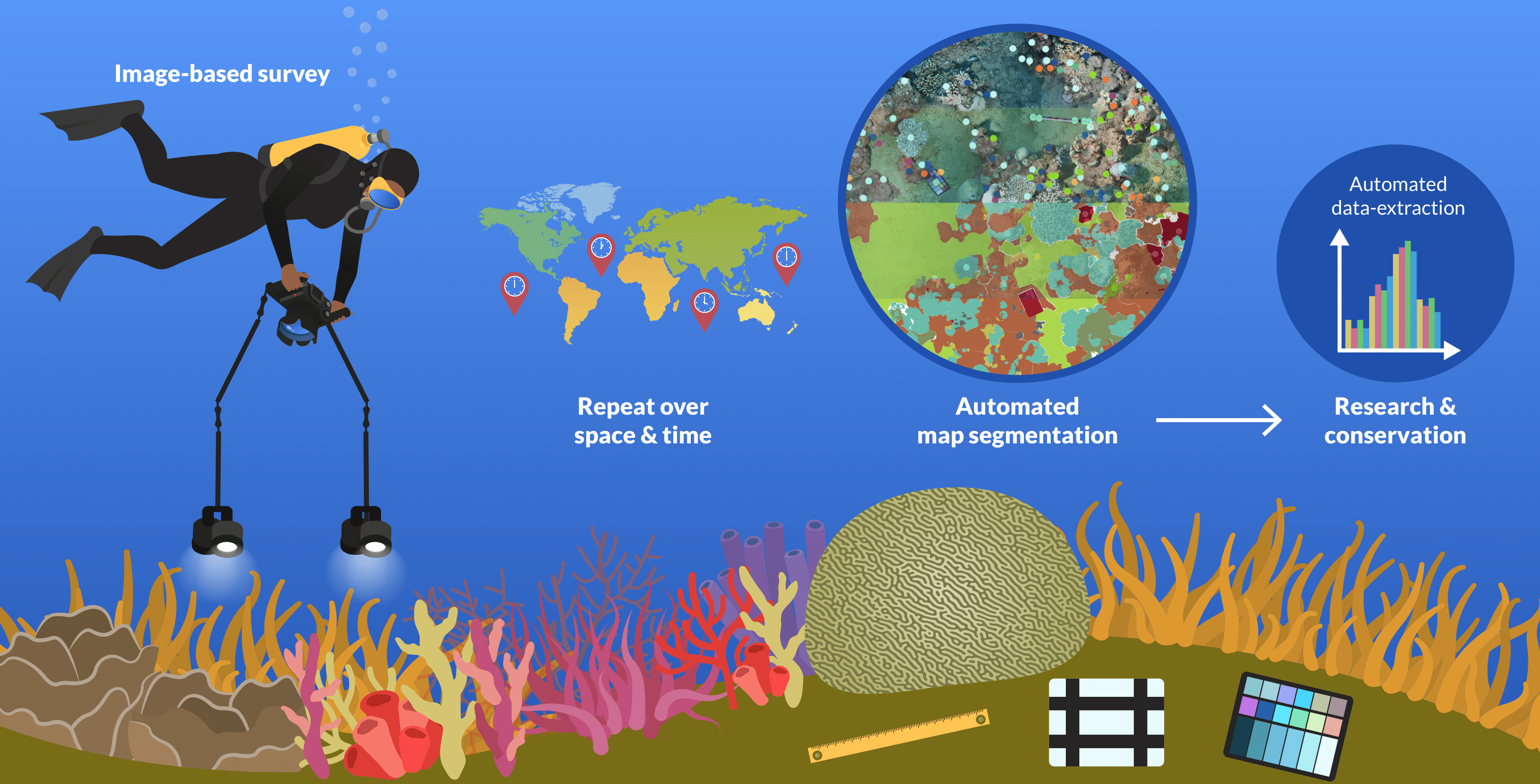
Repeatable Semantic Reef-Mapping through Photogrammetry and Label-Augmentation

1
Hatter Department of Marine Technologies, Charney School of Marine Sciences, University of Haifa, Haifa 3498838 , Israel
2
Department of Marine Biology, Charney School of Marine Sciences, University of Haifa, 3498838 Haifa, Israel
3
Aragón Institute for Engineering Research (I3A), University of Zaragoza, 50009 Zaragoza, Spain
4
ARC Centre of Excellence for Coral Reef Studies, School of Biological Sciences, The University of Queensland, Douglas, QLD 4814, Australia
5
The Mina & Everard Goodman Faculty of Life Sciences, Bar-Ilan University, Ramat Gan 5290002, Israel
6
School of Zoology, Tel-Aviv University, Tel Aviv 6997801, Israel
*
Author to whom correspondence should be addressed.
Current address: Hatter Department of Marine Technologies & Morris Kahn Marine Research Station, Charney School of Marine Sciences, University of Haifa, Haifa 3498838, Israel.
Submission received: 19 January 2021 / Revised: 5 February 2021 / Accepted: 9 February 2021 / Published: 11 February 2021
(This article belongs to the Section Coral Reefs Remote Sensing)

Abstract

:
In an endeavor to study natural systems at multiple spatial and taxonomic resolutions, there is an urgent need for automated, high-throughput frameworks that can handle plethora of information. The coalescence of remote-sensing, computer-vision, and deep-learning elicits a new era in ecological research. However, in complex systems, such as marine-benthic habitats, key ecological processes still remain enigmatic due to the lack of cross-scale automated approaches (mms to kms) for community structure analysis. We address this gap by working towards scalable and comprehensive photogrammetric surveys, tackling the profound challenges of full semantic segmentation and 3D grid definition. Full semantic segmentation (where every pixel is classified) is extremely labour-intensive and difficult to achieve using manual labeling. We propose using label-augmentation, i.e., propagation of sparse manual labels, to accelerate the task of full segmentation of photomosaics. Photomosaics are synthetic images generated from a projected point-of-view of a 3D model. In the lack of navigation sensors (e.g., a diver-held camera), it is difficult to repeatably determine the slope-angle of a 3D map. We show this is especially important in complex topographical settings, prevalent in coral-reefs. Specifically, we evaluate our approach on benthic habitats, in three different environments in the challenging underwater domain. Our approach for label-augmentation shows human-level accuracy in full segmentation of photomosaics using labeling as sparse as 0.1 % , evaluated on several ecological measures. Moreover, we found that grid definition using a leveler improves the consistency in community-metrics obtained due to occlusions and topology (angle and distance between objects), and that we were able to standardise the 3D transformation with two percent error in size measurements. By significantly easing the annotation process for full segmentation and standardizing the 3D grid definition we present a semantic mapping methodology enabling change-detection, which is practical, swift, and cost-effective. Our workflow enables repeatable surveys without permanent markers and specialized mapping gear, useful for research and monitoring, and our code is available online. Additionally, we release the Benthos data-set, fully manually labeled photomosaics from three oceanic environments with over 4500 segmented objects useful for research in computer-vision and marine ecology.

Graphical Abstract

1. Introduction

Accelerations in technologies [1] have empowered ecological studies by facilitating digital representations of natural systems [2], thus reducing uncertainties in predicting their future-state [3]. Advances in computer-vision and remote-sensing enable cross-scale research. In the near future, deep neural networks will help to decipher process-from-pattern as part of automated workflows; preceded by data acquisition from robotic platforms and semantic segmentation of image-based maps [4,5]. Image-based mapping and semantic segmentation are used in an array of ecological studies and applications, ranging from studying vegetation patterns [6,7,8] and city-scapes [9] to farm-management [10]. Specifically, photogrammetry has become a popular approach for benthic research and reef monitoring [11,12,13,14,15,16,17,18,19,20,21]. Structure-From-Motion (SFM) photogrammetry estimates the 3D scene structure and relative motion using subsequent images. It is now possible to view an ecosystem within a digital framework as a continuum across spatial scales, and examine the individuals, populations, and communities that comprise it. Nevertheless, photogrammetry is not yet fully mature as a repeatable method for wide scale ecological surveys. First, the output 3D models and photomosaics need to be labeled rigorously for analysis. This is laborious and requires expert knowledge. Thus, there is an urgent need for automation in the full segmentation task (i.e., labeling each pixel) of photomosaics. Second, a 3D grid needs to be consistently defined for repeated surveys. Without proper data extraction that includes full, pixel-wise classification and labeling, the relevant information remains concealed in the image. Here, we address both issues, providing a more coherent solution for habitat-mapping and underwater photogrammetry. While our methods are applicable to all domains in which photogrammetry is used, here we focus on the benthic environment.
There are increasing efforts for automatic labeling using machine learning [4,6,9,20,22]. However, the commonly used tools [23,24] still provide point classification and not full segmentation. Such sparse sampling is overlooking object/patch level information, such as the morpho-metrics (shape and size) of individual organisms that can be provided by full semantic segmentation. Several methods for segmentation of benthic images and photomosaics have been demonstrated [25,26,27,28,29], including using multi-view images [30] and 3D models [31]. These works that are based on deep learning provide impressive results; however, deep neural networks rely on a high number of learning parameters and because of that, they need to be trained with a large amount of data to avoid overfitting. Then, the main problem for successful automatic identification of marine species is the lack of training data and extensive variability within taxa [32,33] that prevents using labeled data from other locations and predicting labels that were not used in the training data. To overcome this, we propose propagating sparse labels using our Multi-Level Superpixel (MLS) approach [25]. In [25] this method was suggested as a way to quickly generate training data for deep learning semantic segmentation in several terrestrial and underwater domains. Here we show that even by itself it enables obtaining fast full segmentation with minimal human intervention. We test it extensively on photomosaics with respect to ecological measurements and show that it provides very high accuracy. Thus, it can be used as a complimentary method for generating dense training data in cases where there are no available trained deep networks as it is general and not domain specific. Challenges for deep-learning algorithms in underwater imaging include illumination and range, as well as image degradation caused by refraction and wavelength-specific attenuation [34,35]. An orthophoto is generated from a single angle-of-view on the 3D model through the process of orthorectification where a planimetrically correct image is created by removing the effects of perspective (tilt) and relief (terrain). In an orthophoto, the objects are scaled and located in their true positions (topology), enabling direct measurements of areas and distances [36]. However, in transition from 3D to 2D (orthorectification) there are six degrees-of-freedom that need to be set. In topographically complex structures, such as coral reefs, exporting different perspectives of the same 3D model affects the occlusions (Figure 1) and map-topology, as well as artifacting and distortion on non-planar objects with limited input views. Thus, the distance and angle between organisms may differ without consistency in orthorectification. This can be detrimental, for example, in studies regarding neighbor-relations and size-distributions.
Most solutions for defining the plane of projection try to define the Z-axis according to depth in the water-column. Usually, permanent markers such as plastic tubes or steel bolts are used for this purpose [15], and their depth and the distance between them need to be measured directly or indirectly [37]. Other means to solve this problem include towed buoys mounted with GPS sensors [38] in shallow water surveys, and positioning with acoustic data [39]. Yet, these solutions are impractical for deep and remote reef habitats such as Mesophotic Coral Ecosystems (MCEs, 30–150 m depth) [40].
To tackle this problem, we define the Z-axis as the depth axis by placing a spirit leveler within the survey plot and using it to transform the 3D model.
Benthic habitat mapping using acoustic and optic sensors encompassess a range of foci and scales, from species distribution models to community mapping and abiotic habitat mapping [41]. Optical imaging can provide much greater detail than acoustic sensors, which have wider scalability. However, benthic habitats are difficult to map due to the complex interactions between physical, chemical, biological, and behavioral elements that comprise them [42]. Here we present a multi-class community mapping scheme for benthic surveys.
The sessile communities that form and inhabit the reef are linked through cross-scale processes. For instance, in scleractinian corals, growth-rates and neighbor interactions occur at very small spatial scales, yet they operate within a much more expansive system, where dispersion is enhanced by predation and extreme weather events [43], and vicariance is reticulate through ocean currents [44]. Accordingly, both the minute and the enormous scales are significant in characterizing the physical and biological features of reef structures. The composition of taxa in space and time has been the focus of many studies in benthic ecology. However, reefs are so intricate (Figure 2) that in the lack of adequate technology for community-level investigation, the dynamics of sessile organisms remain puzzling. Thus, fundamental questions regarding key ecological processes in the reef have remained largely the same for over five decades [45,46,47,48,49], as a simplified compartmentalization of the benthos is often made for handling complex phenomena.
In ecological studies, the scale of investigation depends on the rate of events [50,51]. Benthic organisms have growth rates on the scale of mms to cms per year [52]. Therefore, our investigation necessitates cm scale change-detection abilities. To assess and validate the change-detection ability of our workflow, we conduct a repeated survey and show that such orthorectification enables consistently examining the growth and decay, spatial topology, and presence/absence counts of sessile reef organisms.
Our methodology for automated and repeatable semantic mapping can detect and relocate sessile organisms on the cm-scale across hundreds of metres. Such a tool can assist in constructing a multi-level, cross-scale view of underwater and terrestrial ecosystems, useful for research and monitoring efforts. In this paper, we describe its application on a new data-set that includes manually segmented photomosaics from three different regions: a rocky reef in the Eastern Mediterranean, a coral reef in the Northern Red-Sea, and a coral community in the Eastern Caribbean. We validate our approach through computer-vision metrics as well as relevant ecological metrics.
Our specific contributions are:
  • Extensive ecological validation of semantic segmentation through label-augmentation of sparse annotations.
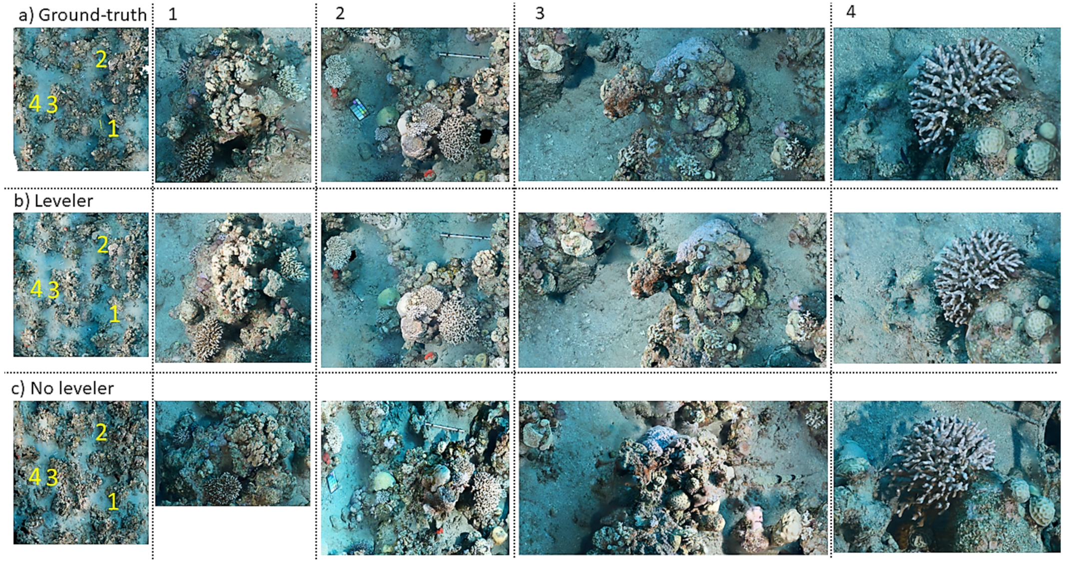
  • Validation of 3D grid standardisation with a consumer-grade spirit-leveler.
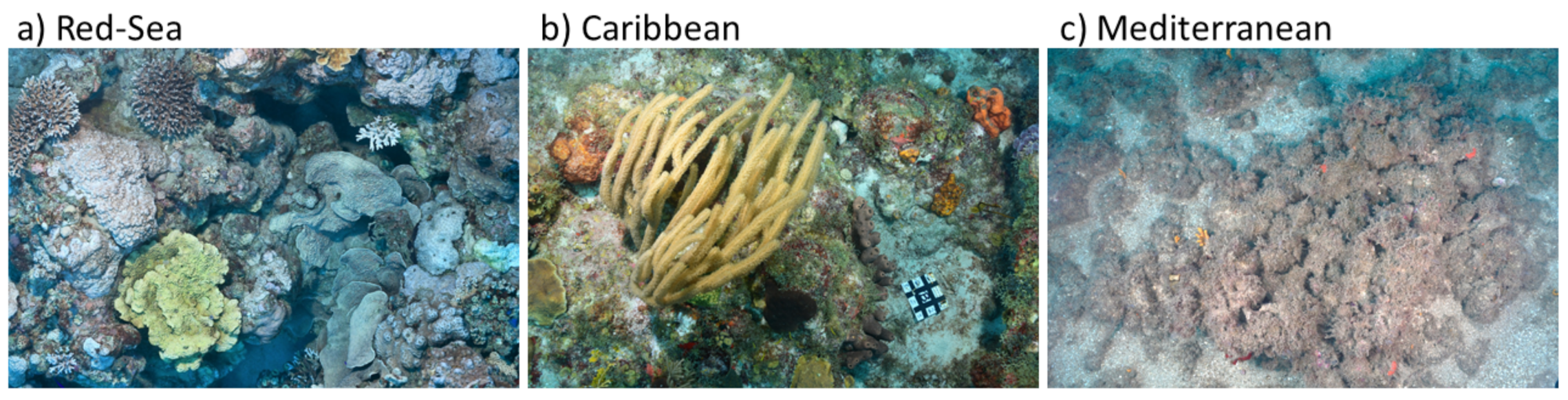
  • The Benthos data-set that includes three segmented photomosaics from different oceanic environments.

2. Materials and Methods

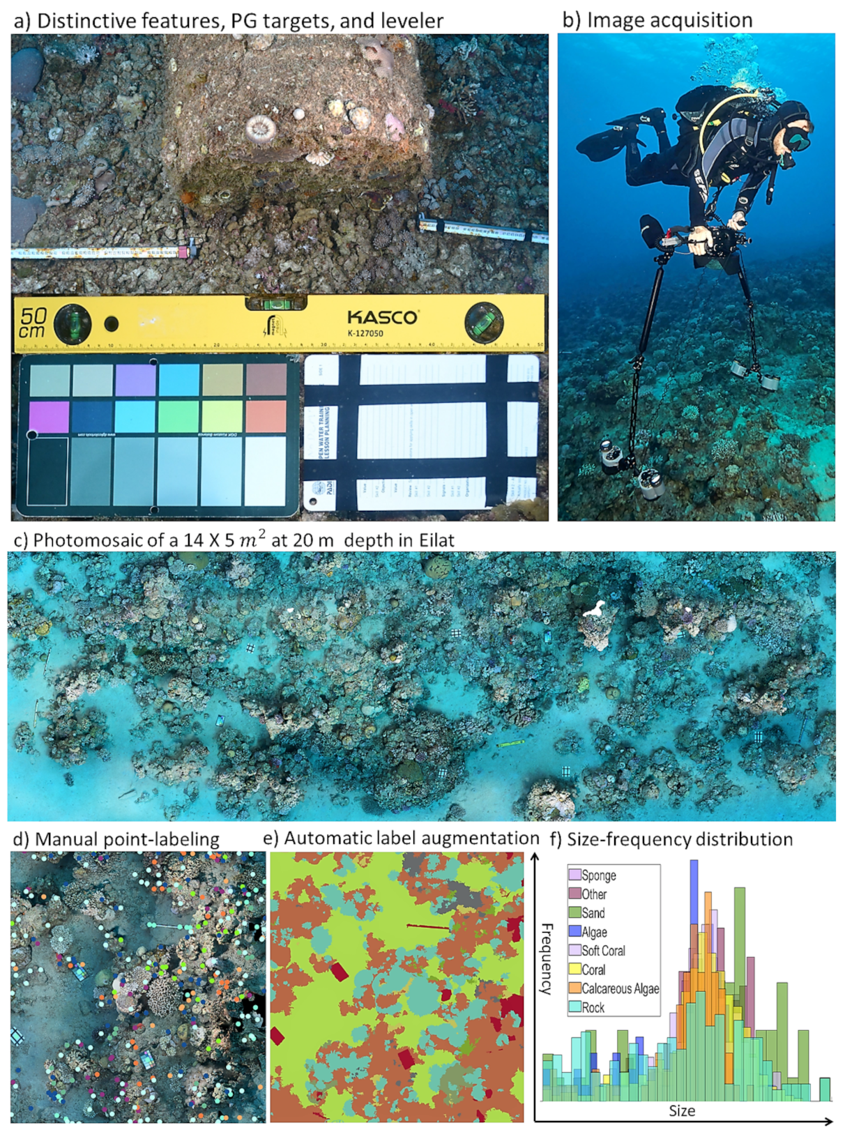
2.1. Imaging System and Photogrammetric Equipment

A NIKON D850 camera with a 35 mm NIKKOR lens in a Nauticam housing with four INON Z-240 strobes was used (Figure 3b). Photogrammetric targets are objects with distinguishable features and orientation. Our targets included measuring tapes, 0.5 m scale-bars, underwater colour charts (DGK), a spirit leveler, and dive slates with electrical tape markings (Figure 3a).

2.2. Plot Setup and Acquisition Protocol

When reaching the target depth, a distinguishable natural or artificial object which is relatively simple to navigate to was detected as a starting point for the survey. From that point, we measured the required transect length (5–30 m) using a measuring tape and marked its surroundings using photogrammetric targets and scale bars. In the orthorectification experiments, we aligned a spirit leveler in the survey plot. The spirit leveler has three bubble indicators (Figure 3a). When it is placed in such a way that the bubbles are centred, the leveler can be used to define a plane-of-projection. Optimally, the leveler was placed in the centre of the plot, and parallel to the transect. The leveler is used to transform the 3D model, thus it is paramount to obtain a good reconstruction of it by acquiring many (>15) images from different angles and distances.
Before each survey, several test images were taken to adjust camera settings: ISO, aperture, shutter speed, and focus. When reaching the optimal camera settings the survey was initiated, and settings were not changed throughout it. Images were acquired at 1 Hz using the camera’s interval timer shooting function. The camera was held mainly downward-looking while the diver swam in a lawn-mower (boustrophodonic) pattern, performing close reciprocal passes over the survey plot to ensure overlap between parallel legs.

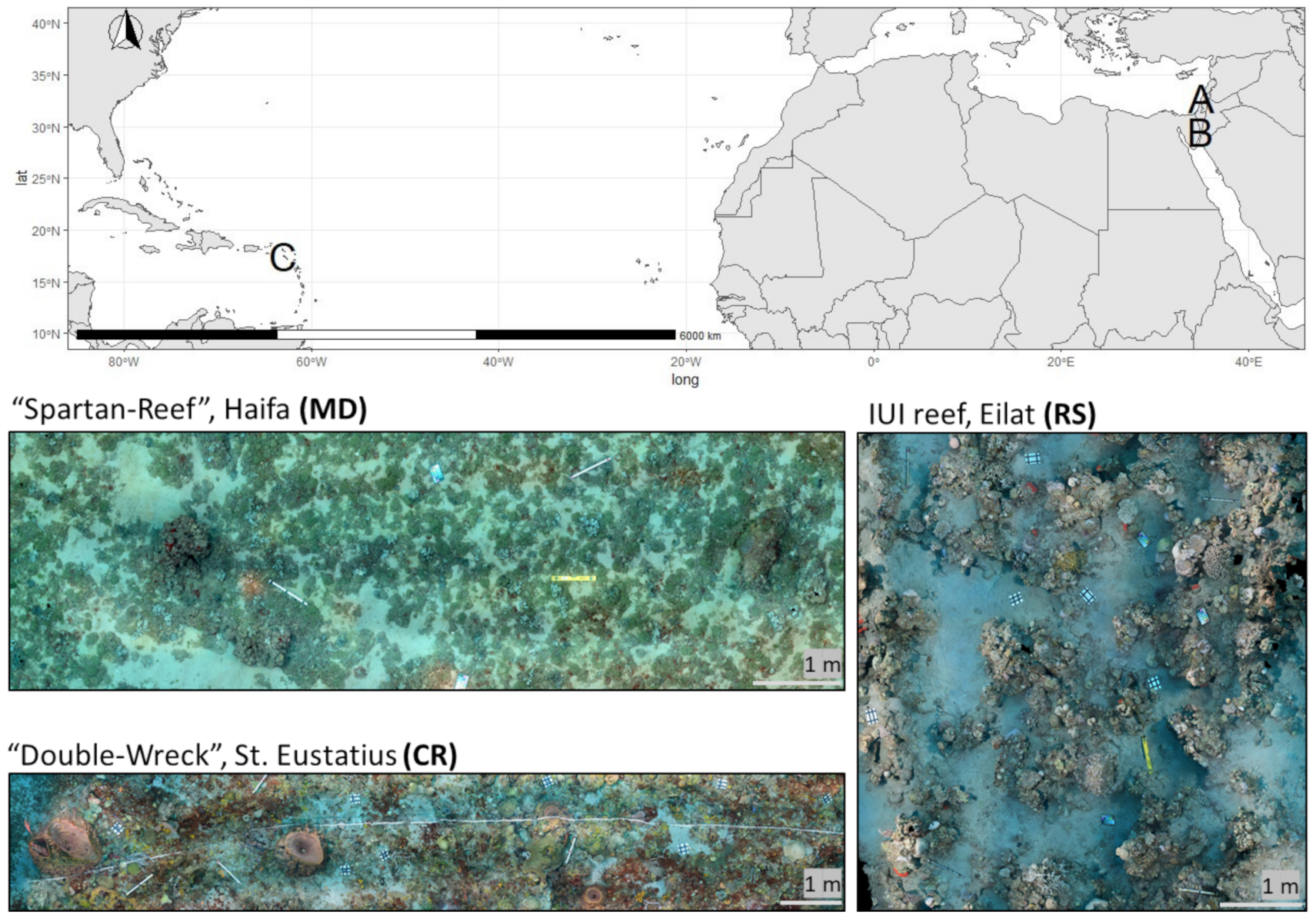
2.3. Study Sites and Data-Sets

We used image-sets from three distinct oceanic environments (Figure 2 and Figure 4). This comes to show the implementation of our workflow in different ecological zones, and demonstrate the generality of this method (Table 1).

Labeling and Classification

We used two manual labeling schemes: coarse labeling (a polygon inside the object covering its centre but not all of its pixels) and full segmentation, and two classification schemes: genus-specific (57 classes), and habitat mapping (eight classes) (Table 1). We used labelbox, a dedicated tool for computer-vision applications, because of its flexibility, academic pricing benefits, and simple interface. Images were uploaded and labeled with a polygon project setup. In data-set Red Sea 20 (RS20) we used genus-specific classes for scleractinian corals, and other sessile groups at lower taxonomic resolutions. In data-sets Red-Sea (RS), Caribbean (CR), and Mediterranean (MD) we used eight classes in full manual labeling, by the terrain type. This requires less expertise and can be distributed among non-expert labelers such as under-graduate or high-school students, and even external workforces.

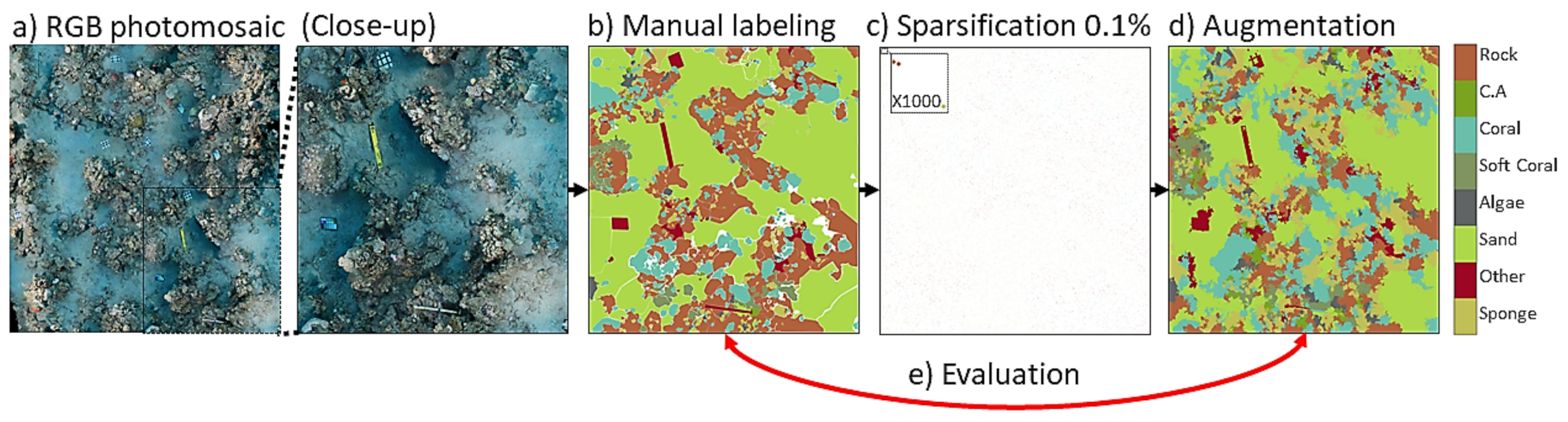
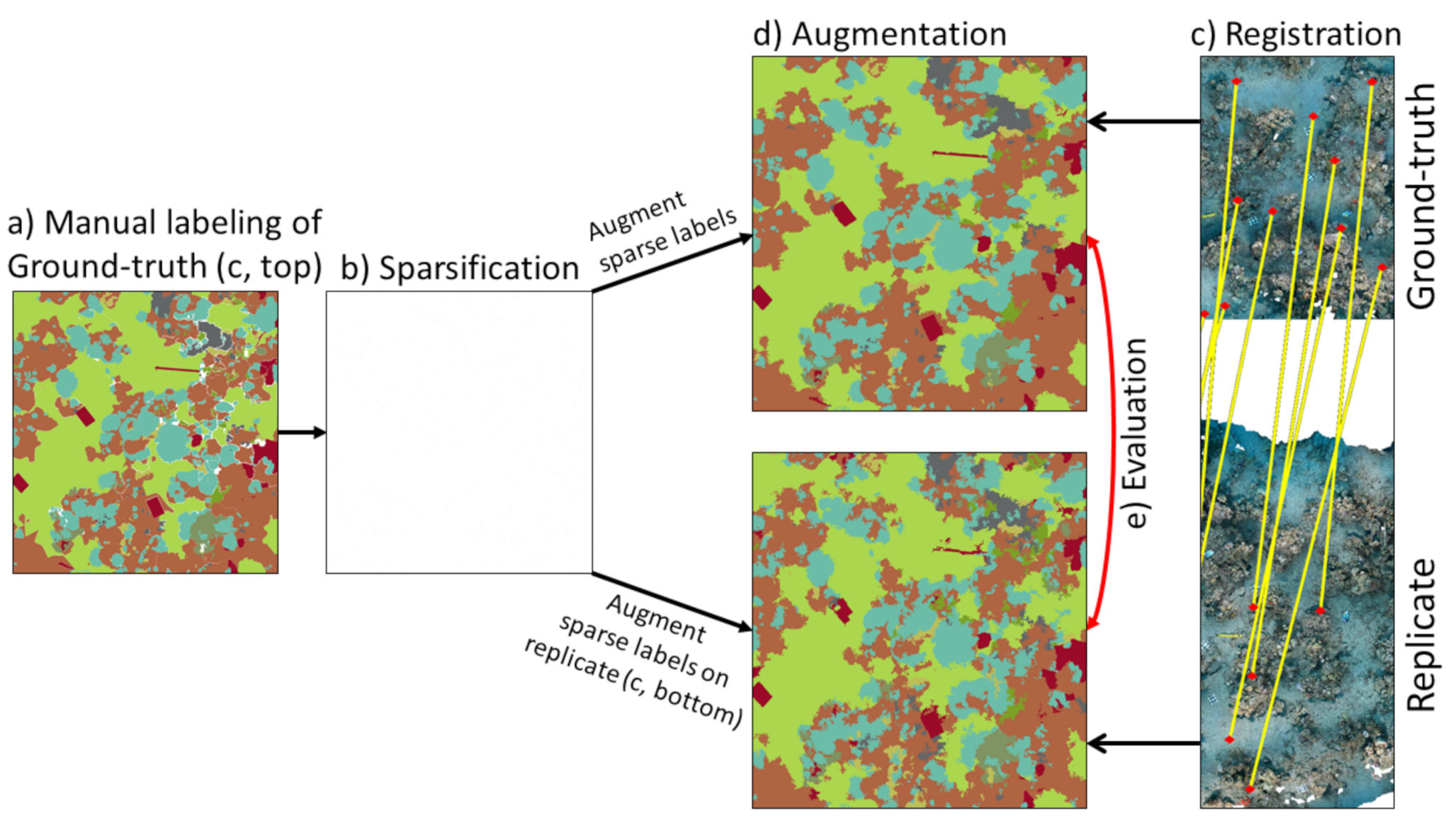
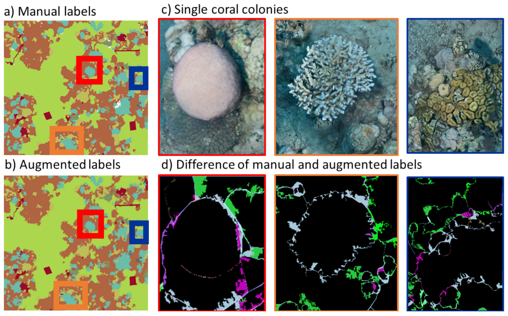
2.4. Label-Augmentation

This experiment reflects the amount of labeling effort required in order to obtain the highest quality of label-augmentation.

Augmentation from Sparse Annotations

Label-augmentation consists of expanding sparse labels to full segmentation by augmenting the number of labeled samples. We use the method previously developed by us [53] that was since validated extensively on different types of data including city-scape images for autonomous driving, terrestrial orthophotos, and fluorescent and RGB coral images [25,54] (code available online https://github.com/Shathe/ML-Superpixels (accessed on 19 January 2021)). Here, we examine this method with respect to meaningful ecological measures. We apply label-augmentation on photomosaics (Figure 5), where the input is sparse annotations, and the output is a fully segmented map. A superpixel is a low-level grouping of neighboring pixels. The MLS approach uses superpixels to propagate the sparse labels. It computes several superpixel levels of different sizes and uses the sparse annotations as votes. It consists of applying the superpixel image segmentation iteratively, progressively decreasing the number of superpixels generated in each iteration. In the first iteration, the number of superpixels is very high, leading to very small-sized superpixels for capturing small details of the images. The following iterations decrease the number of superpixels, leading to larger superpixels covering unlabeled pixels. Successive iterations do not overwrite information; they only add new labeling information until all pixels are covered.
To evaluate the method, we conducted an experiment to estimate how many initial seeds are required to achieve an accurate full segmentation and how different sparsities affect the augmentation performance. As our photomosaics were manually labeled densely, i.e., all the pixels were labeled, we simulate the sparse labeling by randomly sampling initial seeds in several sparsity levels (10%, 1%, 0.1%, 0.01%, 0.001%) of the original dense labels, and augmenting it using the same method. These sparse labels simulate the way benthic data-sets are usually labeled for reducing the labeling cost.

2.5. Orthorectification

The purpose of this experiment was to simulate repeated surveys without permanent markers or navigation sensors. In this manner, repeated surveys can take place with the aid of natural and artificial references such as distinctive reef features or mooring sinkers. These objects serve as a starting point for the survey, and orthophotos can be registered in post-processing as long as they are consistently orthorectified.

2.5.1. 3D Grid Definition and Orthorectification

We used Agisoft Metashape 1.5 for constructing the 3D map models and orthophotos (Agisoft Metashape Professional Version 1.5, Agisoft LLC, St. Petersburg, Russia, 2016). In data-sets RS20, RS, and MD, a 0.5 × 0.05 m 2 spirit leveler was used to define the 3D grid. The models were scaled using the known size of the scale bars. We marked the points of known distance on 5–10 images until the scale error was lower than 0.0005 m. Exporting the orthophoto has several degrees-of-freedom that have to be set for repeatability. The locations of three corners of the spirit leveler were marked as ( X , Y , Z ) = ( 0 , 0 , Z ) , ( 0 , 0.05 m , Z ) , ( 0.5 m , 0 , Z ) where Z is the known depth measured in situ. This was done within the reference pane of Agisoft, marking 15–20 images from different angles and distances. The model was then rotated and translated accordingly, and a photomosaic was exported. Orthorectified photomosaics were exported as .png image files at a resolution of 0.5 mm per pixel. These were then cropped to the area of interest and adjusted for contrast in Matlab using the imadjust function [MATLAB R2019].

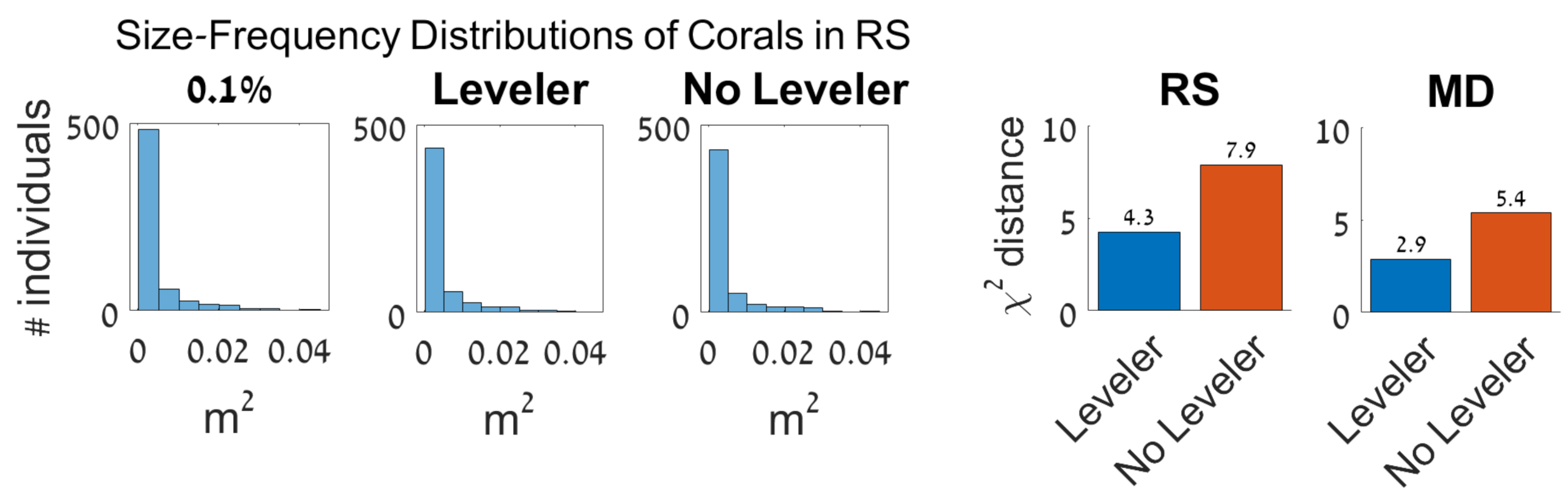
2.5.2. Repeated-Survey Simulation

To estimate the ability of our pipeline for orthorectifying using a leveler and its change-detection sensitivity we repeated image acquisition two to three times during the same dive, resulting in image sets that constitute technical replicates. Between repeats, the spirit leveler was moved around the scene. The ground-truth photomosaic represents a first temporal repeat or baseline survey, and it was fully manually labeled. The labels were then sparsified (subsampled), and augmented on all replicates resulting in fully segmented photomosaic replicates. These were compared to the ground-truth mosaic for evaluation (Figure 6e).
In this experiment our replicates are expected to be identical and the negative-control (naïve) is expected to show the highest variance from the ground-truth. To generate the naïve (no leveler) photomosaic, one of the image-sets was exported twice, before and after transformation. We registered the replicate orthophotos using Matlab’s manual image registration tool cpselect and 15–20 registration points (Figure 6c).

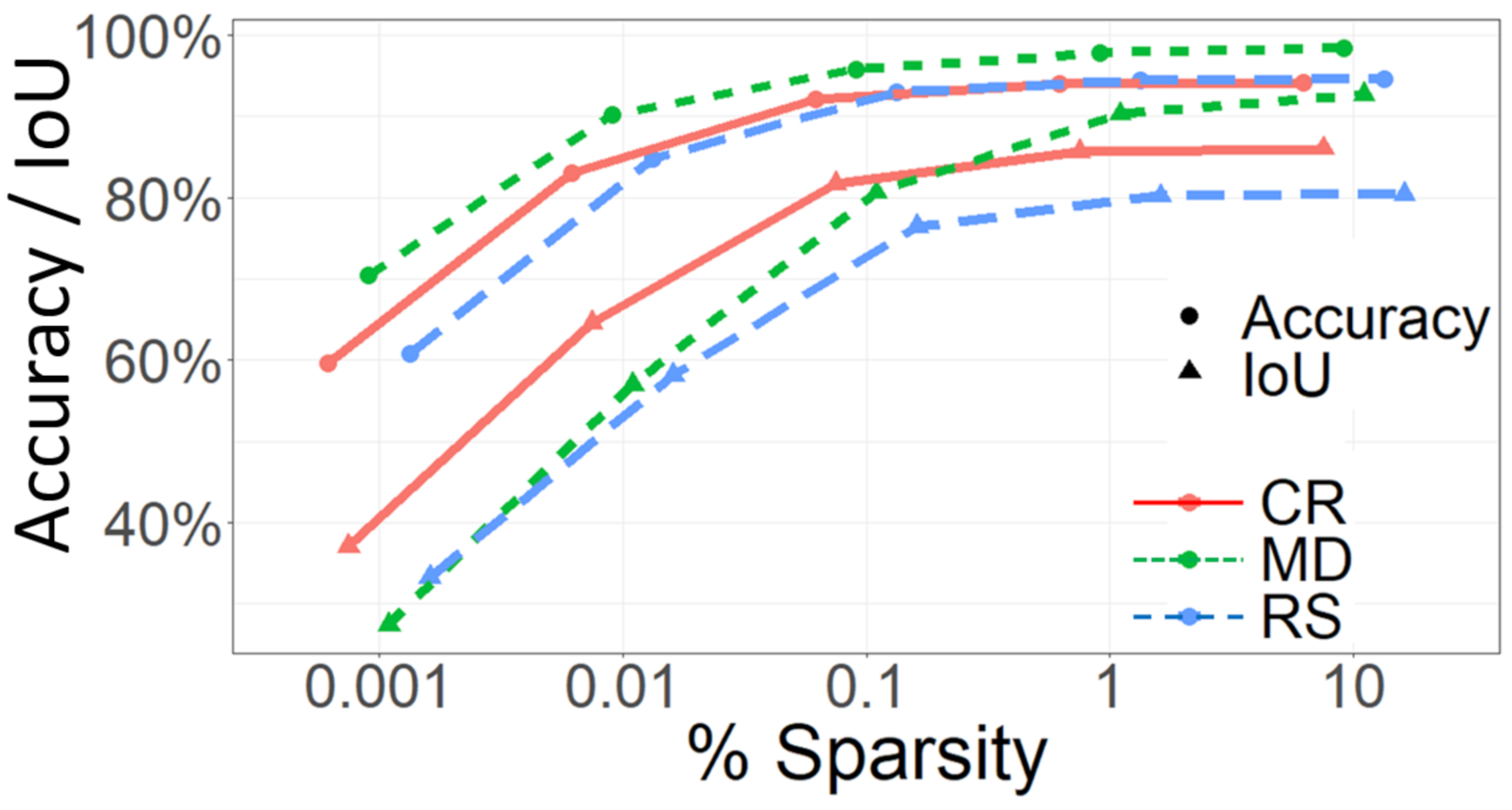
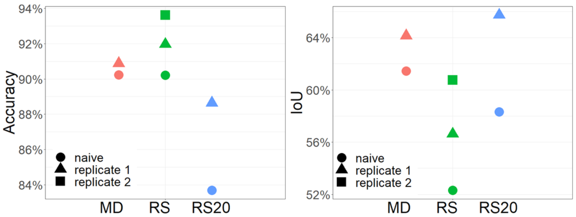
2.6. Evaluation Metrics

In all augmentation experiments, the augmented labels were evaluated against the original manual dense annotations. Several metrics were used to assess the performance of the augmentation including recall, accuracy (per pixel) and the Intersection over Union (IoU, per class):
Recall = True Positives True Positives + False Negatives
Accuracy = True Positives + True Negatives True Positives + True Negatives + False Positives + False Negatives
IoU = True Positives True Positives + False Positives + False Negatives
These metrics are normally used to assess the performance of CNNs in segmentation tasks.

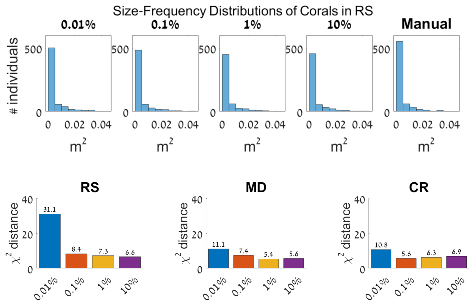
2.7. Community-Metrics Comparisons

We developed a Matlab code for community data extraction. All the objects below size 0.0002 m 2 were excluded from analysis because they come from noise in the segmentations.
  • Class-specific size-frequency distributions. We divided the classes in nine bins, starting from 0.0002 m 2 to 0.045 m 2 with a step size of 0.005 m 2 . We used χ 2 distance to assess the similarity of class size distribution between maps. Low values indicate high similarity between sets of data where zero is the maximal similarity.
    χ 2 Distance = i = 1 n ( Observed i Expected i ) 2 Observed i + Expected i
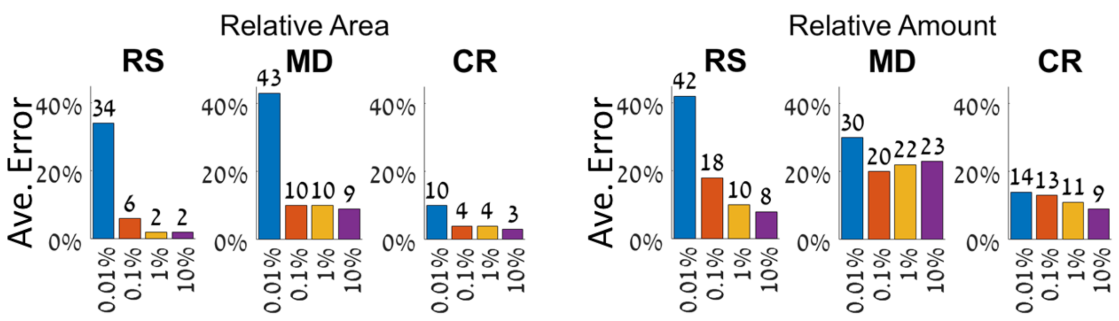
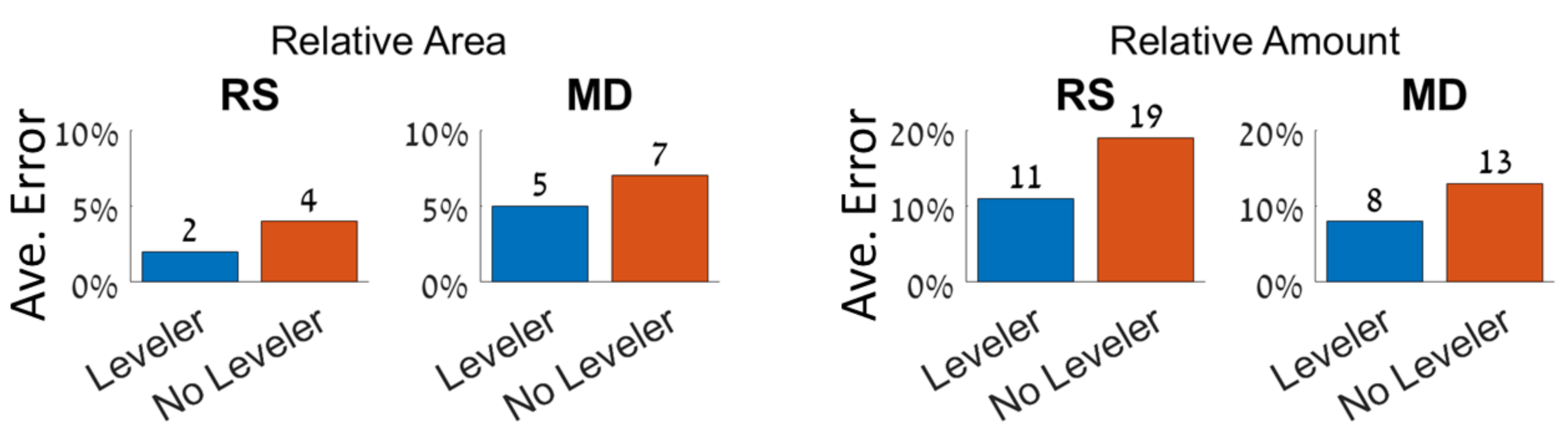
  • Relative amount of individuals per class. The number of objects from each class divided by the total number of objects in the map.
  • Relative area by class. The size in m 2 per class divided by the total size of the map. The photomosaics are exported at 0.5 mm per pixel, and to transfer to m 2 we use the following equation:
    Size in m 2 = Pixels 4 × 10 6

3. Results

3.1. Label-Augmentation

In this experiment we used fully manually labeled images to test the MLS augmentation approach from sparse seeds on wide scale data; photomosaics from different reef environments. We used data-sets RS, MD, and CR. The label-augmentation experiment shows that augmented labeling and dense manual annotations provide very similar ecological outputs. Figure 7 depicts both the per-pixel accuracy and the IoU for all sparsity levels. The per-pixel metric (accuracy) is higher because of the background classes (Sand, Rock) that have a larger area. Please note that this means that the per-pixel metrics are biased towards dominant classes. The per-class metric (IoU) is lower because of small biotic classes which are more difficult to augment. Per-class metrics take more into account the small ones, which usually have worse results because they are harder to propagate/augment. Even though, these metrics show that we can properly propagate sparse labels even for small classes. For both metrics it can be seen that the sparsity of 0.1% is optimal, as investing time in annotating beyond this sparsity level does not provide a serious gain in augmentation quality both in terms of accuracy and IoU.
The χ 2 distance was calculated between the class-specific size-frequency distributions (e.g., Figure 8 left), and averaged over eight classes in each mosaic replicate and its manual labels (ground-truth). The distance values are low and there is no significant decrease in distance above sparsity 0.1%. In data-set CR, the trend is even slightly reversed (Figure 8 right). In relative area (Figure 9 left), the error values are low and there is no serious decrease in error above sparsity 0.1%. The error for sparsities 0.1–10% ranges from two to ten percent. In relative amount (Figure 9 right), the errors decrease above sparsity 0.1% in the RS and CR data-sets, but not in the MD data-set. The error for sparsities 0.1–10% is low and ranges from eight to 20 percent.
The label-augmentation experiment shows that the segmentation improves with denser seeds, most significantly up to 0.1% sparsity, where annotations denser than 0.1% do not provide serious increase in accuracy. The effect of sparsity on the error in community metrics was slightly different between data-sets. Noticeably, the RS data-set was most affected by percent sparsity since it is the most topographically complex reef, with clearer trends of decrease in error with denser seed-labels. These results mean that to obtain a reliable segmentation, the amount of required labeling is above 0.1% of the pixels. Label-augmentation is an important contribution as an efficient sparse to dense approach for image- segmentation and alleviates the effort in generating training data for deep learning applications. Ideally, the best way to augment labels is from point annotations of each object in the image, because the augmentation propagates seed labels. Therefore, an object that is not labeled, will not show on the augmented image, and will be overridden by neighboring labels. In labeling, even humans fail to accurately label objects along the edges and our accuracy in augmentation was affected by the segment edges where most of the errors occur.Figure 10 shows the manual and augmented labels of the RS data-set, with close-up views on single coral colonies.

3.2. Orthorectification

The orthorectified photomosaics were superior to the naïve photomosaics in accuracy and IoU throughout all data-sets (Figure 11). The χ 2 distance was calculated between the class-specific size-frequency distributions (e.g., Figure 12 left), and averaged over eight classes in each mosaic replicate and its augmentation from sparsity 0.1% (ground-truth). In the orthorectification experiment (Figure 12 right) the orthorectification using a leveler reduces the distance between the naïve and orthorectified histograms.
In relative area (Figure 13 left) the orthorectification increases accuracy. Error was calculated as the ratio between each replicate and the ground-truth mosaic (multiplied by 100). The error for photomosaic that have been orthorectified ranges between two to five percent, and for the naïve photomosaics from four to seven percent, with similar effect in both data-sets. In relative amount (Figure 13, right) the orthorectification increases the accuracy. The error for photomosaics that have been orthorectified ranges between eight to 11 percent, and for the naïve photomosaics from 13 to 19 percent, with more effect in the RS data-set. The orthorectification experiment shows that for both data-sets the error in size-frequency distribution as well as relative size and amount decreased when the maps were orthorectified. This is a clear trend in which the naïve orthomosaics are inferior in repeatability to the orthorectified replicates. We found that the effect of orthorectification on the augmentation results was stronger on topographically complex reefs where more occlusions occur. Furthermore, despite small differences in accuracy (Figure 11), the presence/absence data as well as the topology of the maps differs significantly (Figure 10). Such artifacts generated by inconsistent orthorectification are inimical for studies interested in tracking single coral colonies over time.

4. Discussion

We presented a methodology for cm-scale change-detection, solving two main issues: swift data-extraction and consistent 3D grid definition. We used the MLS approach for label-augmentation on photomosaics, and a 3D transformation of the map using a spirit leveler placed in the scene. We used image-sets from three distinct oceanic environments, implementing our workflow as a general and robust method in different ecological zones (Figure 4, Table 1). The results support our method as a practical, rapid, and cost-effective solution that can be applied at the reef-scape scale with colony level resolution.
Labeling the RS and CR data-sets was difficult due to the large amount of small segments. The CR data-set also had a large amount of non-rigid corals and strong surge currents during image acquisition, resulting in reconstruction artifacts. In all data-sets, we found that it is important to label the objects close to the edges.
Label-augmentation is useful because it opens the possibility to augment previously labeled data with minimal adjustments. In that case, the detection ability in augmenting labels from sparse annotations will be at the resolution of the spacing between labels. Although 0.1% sparsity might take longer than the traditional random point annotation, it is important to note that we showed it yields significantly more data and therefore worth the added time. In addition, when labeling the orthophotos using polygons it requires only <10 clicks per object and yields more than 0.1% sparsity.
In the orthorectification experiment we tested whether 3D grid definition using a spirit leveler is superior to a non-intervention, naïve approach, and provides stable results.
Before deciding on the leveler method, we also tried to use a line and a float with weights for finding the Z-axis, but it does not reconstruct well in the model and is susceptible to currents. Alternatively, we thought on using corner-shaped aluminum bars linked to permanent markers, which are intrusive and can be inconsistent due to subtle movements of the seabed. We also tried to measure the depth at the corner and centre of the plot which proved to be time-consuming and less practical.
To conclude, slope angle and topographical complexity are the key factors that increase the necessity of this kind of approach for consistent 3D grid-definition. A two to five percent error in the orthorectification experiment translates into a cm change-detection threshold in real-world applications such as coral reef monitoring.
Full consistent semantic mapping brings forth unprecedented level-of-detail that will pave the way for a new generation of highly detailed ecological studies. Yielding extensive community metrics automatically is one of the main motivations of photogrammetric surveys. Here, we streamline and enhance the volume of information extracted automatically from photomosaics.
We successfully detected and classified organisms as small as two cm 2 . However, orthorectification generates artifacts such as blur and holes which also affect size/area measurements. We designed our workflow to be robust and adaptable rather than domain-specific which is often the case with deep-learning and limited training-data. As our analysis shows, the commonly used accuracy and IoU evaluation metrics often do not tell the whole story, as ecological metrics provide a more comprehensive evaluation. Therefore, our evaluation criteria are useful for testing other image segmentation approaches as well.
Although this workflow is customized for an underwater setting, it is widely transferable. Previously, label-augmentation through the MLS approach was established to facilitate training semantic segmentation [25,53,54] and was demonstrated on multiple domains such as multi-modal images of corals and terrestrial orthophotos with similar accuracy, showing the generality and the wide range of problems that can be handled with this approach. Thus, this work is significant for all ecologists that wish to use photogrammetry in their research. Object Based Image Analysis (OBIA) has been used extensively in remote sensing [55] and benthic habitat mapping [56,57,58,59]. As long as the object of interest is larger than the pixel size, it can be delineated as a group of pixels. Here we use an adaptive-Superpixel approach- MLS, which can also be considered to be an object-based Image analysis scheme. At the cm scale resolutions of benthic organisms, we require high resolution data to employ such object oriented image analysis schemes, which can be provided by photogrammetric surveys with sub cm resolution across tens of metres.
Shortcomings and remaining challenges for robust automatic surveys include lack of specific algorithms for underwater photogrammetry that take into consideration non-rigid organisms such as soft-corals in surge currents, and analysis of 3D photogrammetrical outputs [31,60,61]. Many studies have used 2D maps, photomosaics, instead of 3D data; point-clouds or surface-mesh which are also generated in the photogrammetric process. This reduction is made to simplify the technical aspects of data-analysis (labeling in 3D) in the lack of adequate software and workflows. Relative abundance (amount) and relative area (Figure 9 and Figure 13) metrics are important for ecological studies because they reflect diversity and evenness measures as well as the well-being of the reef. Furthermore, since object level separation is still ambiguous in photomosaic analysis (due to occlusions and angle-of-view), area measurements are more reliable than individual counts and allow estimating the percent live-cover. A main drawback in photomosaics is that even with consistent orthorectification there are occlusions and size distortions (artifacts) of non-planar objects that make measuring individual reef organisms challenging. An inherent limitation in orthophotos is that they fail to depict crevices, overhangs, and other non-planar reef formations. Therefore, some organisms are not represented proportionally in ecological estimations based on orthophotos. Nevertheless, they are still the prevalent tool for such estimates because of their advantages; scalability and resolution. Future studies should focus on deriving community metrics of benthic habitats using the full suite of visual information in photogrammetric surveys; linking the high-resolution information contained in the input images for the Structure From Motion (SFM) process across a wide scale 3D map.
One of the biggest challenges in achieving a taxonomic segmentation of the seabed is the intricacy of the benthos. Sessile invertebrates often do not have clear boundaries, and display overgrowth patterns which are difficult to classify. In such cases, even manual segmentation would not be accurate. Specific algorithms for underwater image enhancement [62] might improve edge detection algorithms, and enable better segmentation. Moreover, there still remains significant work to be done on accurate placement of underwater photomosaic on GPS coordinates [37,63]. This would benefit reef ecology because benthic-mapping would become easily repeatable between teams as well as more precisely comparable across geographic grids. This is normally done using permanent markers or navigation sensors such as GPS buoys which are only effective for shallow reefs. Diver-held navigation tools such as underwater tablets (e.g., http://allecoproducts.fi/about/, https://uwis.fi/en/ (accessed on 19 January 2021)) are emerging, and will complement photogrammetric surveys in the near future.
Classification of the benthos is one of the most important aspects of marine research and conservation, and underwater photogrammetry can supplement other modalities in benthic habitat mapping. For example, [64] combined acoustic and visual sensors to produce a wide scale bathymetry coupled with high resolution photomosaics from video. Furthermore, Multibeam echosounders are becoming popular for indicating seabed substrate type. However, they still require calibration across sites and devices [65]. Spectral features obtained in acoustic surveys have also been shown to be a predictor for terrain type in acoustic habitat mapping. However, these also require ground truthing [66], which can be done using photomosaics. Adaptive workflows that combine acoustic and visual sensors will enable complex navigation tasks with multimodal data. For example, an acoustic survey can find points of interests followed by a close-up visual survey. This will not only benefit ecological surveys and habitat depiction but also development of new algorithms for Multi-modal Simultaneous Localization and Mapping (SLAM).

5. Conclusions

We presented our work on benthic mapping and accelerated segmentation through photogrammetry and Multi-Level Superpixels, and showed the accuracy of repeated surveys using orthorectification and sparse label augmentation. We included objects as small as 2 cm 2 and shown that our method provides fast and reliable segmentation across scale. This approach is appropriate for any person who is interested in using photogrammetry for ecological surveys, especially diver-based underwater surveys (i.e., transects, reef-plots).
Photogrammetry is gaining traction among marine ecologists and map-models of the benthos have outstanding resolution and scaling abilities. Diver-based photogrammetry is possible to conduct without extensive expertise or specialized equipment and is becoming a key tool in the benthic ecology toolbox. With meaningful annotations, photomosaics of the reef can capture the size, shape, and location of hundreds of individual reef organisms. Thus, the bottleneck in ecological studies is shifting towards analysis over acquisition. With advances in acquisition and computer-processing abilities, it is of great importance to explore new ways for data extraction, and the automation of classification and labeling needs to be integrated into marine surveys. Label-augmentation enables serious time savings for complete scene understanding and measurements at the individual-to-population level, such as size-frequency distribution and relative abundance. However, to compare complementing maps over time, standardization needs to be made in terms of consistent 3D grid definition; especially on topographically complex reefs.
We conducted repeated surveys of the same reef plot at minimal intervals of a few minutes assuming no actual change in the terrain in this time-frame, following this assumption, we expected the photomosaic replicates to contain identical ecological information. However, comparing the similarity of orthophotos is not straightforward, due to differences such as color and artifacts (blur/holes) caused for example by slight differences in the distance and angle of image. We compared the maps indirectly through label-augmentation. Comparing the segmented maps generated from augmenting a single set of sparse labels (from the original image) tests all steps of the workflow intact, and includes noise from the photogrammetric (different input images) and orthorectification processes. Thus, it simulates an observer effect and a noisy real-world situation.
When applying this workflow in any setting, the most important factors to consider are the classification level (taxonomic/functional specificity), as it implies on the level of expert knowledge required as well as the accuracy in automatic identification, and the expected change-detection ability which is governed by the effective resolution and signal-to-noise ratio. Furthermore, it is important to consider the effect of the slope on the reef, in the sense that the top down view is not always perpendicular to the reef-table.
At the moment, there are several tools for image segmentation with weak human-interference [67]. Moreover, new tools will soon be released with promising outlook on the benthic photomosaic segmentation tasks [68].

Author Contributions

Conceptualization, All Authors; methodology, M.Y., T.T., I.A., and A.C.M. validation, M.Y. and I.A.; formal analysis, M.Y., I.A., T.T., and A.C.M.; investigation, M.Y., I.A.; resources, M.Y., T.T., I.A., and A.C.M.; data curation, M.Y., T.T.; writing—original draft preparation, M.Y., I.A., T.T.; writing—review and editing, All authors; visualization, M.Y., I.A.; supervision, T.T., D.T., A.C.M.; project administration; M.Y.; funding acquisition, M.Y., T.T. All authors have read and agreed to the published version of the manuscript.

Funding

T.T. was supported by the The Leona M. and Harry B. Helmsley Charitable Trust, The Maurice Hatter Foundation, the Israel Ministry of National Infrastructures, Energy and Water Resources Grant 218-17-008, the Israel Ministry of Science, Technology and Space grant 3-12487, and the Technion Ollendorff Minerva Center for Vision and Image Sciences. I.A. and A.C.M. were supported by project PGC2018-098817-A-I00 MCIU/AEI/FEDER, UE. M.Y. was supported by the PADI Foundation (application #32618), the Murray Foundation for student research, ASSEMBLE+ European Horizon 2020 (transnational access #216), and Microsoft AI for Earth; AI for Coral Reef Mapping. Y.L. was funded by the Israel Science Foundation (ISF) grant No. 1191/16. GE was supported by the European Union’s Horizon 2020 research and innovation program under the Marie Skłodowska-Curie grant agreement #796025.

Data Availability Statement

The Benthos data-set and Matlab code is available in the Dryad Digital Repository: https://0-doi-org.brum.beds.ac.uk/10.5061/dryad.8cz8w9gm3 The code for ML Superpixels can be found at: https://github.com/Shathe/ML-Superpixels.

Acknowledgments

We thank the Morris-Kahn Marine Research Station, the Interuniversity Institute for Marine Sciences of Eilat, and the Caribbean Netherland Science Institute for making their facilities available to us, and most importantly the students, staff, and diving teams of these facilities for fieldwork and technical assistance; Aviad Avni, Deborah Levi, Assaf Levi, Opher Bar-Nathan, Leonid Dehter, Yuval Goldfracht, Sharon Farber, Ilan Mardix, Inbal Ayalon, Liraz Levy, Lindsay Bonito, Pim Bongaerts, Bashar Elnashaf, Derya Akkaynak, and Avi Bar-Massada for valuable intellectual and technical contributions; The image labeling team: Shai Zilberman, Gal Eviatar, Adi Zweifler, Oshra Yossef, Matt Doherty; Guilhem Banc-Prandi for the picture in Figure 3b; Netta Kasher for drawing the graphical abstract; NVIDIA Corporation for the donation of the Titan Xp GPU used in this work. Fieldwork in Eilat was carried out under permit #42-128 from the Israeli Nature and Parks Authority.

Conflicts of Interest

The authors declare no conflict of interest.

References

  1. Kurzweil, R. The law of accelerating returns. In Alan Turing: Life and Legacy of a Great Thinker; Springer: Berlin/Heidelberg, Germany, 2004; pp. 381–416. [Google Scholar]
  2. Davies, N.; Field, D.; Gavaghan, D.; Holbrook, S.J.; Planes, S.; Troyer, M.; Bonsall, M.; Claudet, J.; Roderick, G.; Schmitt, R.J.; et al. Simulating social-ecological systems: The Island Digital Ecosystem Avatars (IDEA) consortium. GigaScience 2016, 5, s13742-016. [Google Scholar] [CrossRef] [PubMed] [Green Version]
  3. Laplace, P.S. A Philosophical Essay on Probabilities, Sixth French ed.; Truscott, F.W.; Emory, F.W., Translators; Chapman & Hall, Limited: London, UK, 1902. [Google Scholar]
  4. Brodrick, P.G.; Davies, A.B.; Asner, G.P. Uncovering ecological patterns with convolutional neural networks. Trends Ecol. Evol. 2019, 34, 734–745. [Google Scholar] [CrossRef]
  5. De Kock, M.; Gallacher, D. From drone data to decision: Turning images into ecological answers. In Proceedings of the Conference Paper: Innovation Arabia, Dubai, United Arab Emirates, 7–9 March 2016; Volume 9. [Google Scholar]
  6. Kattenborn, T.; Eichel, J.; Fassnacht, F.E. Convolutional Neural Networks enable efficient, accurate and fine-grained segmentation of plant species and communities from high-resolution UAV imagery. Sci. Rep. 2019, 9, 1–9. [Google Scholar] [CrossRef]
  7. Silver, M.; Tiwari, A.; Karnieli, A. Identifying vegetation in arid regions using object-based image analysis with RGB-only aerial imagery. Remote Sens. 2019, 11, 2308. [Google Scholar] [CrossRef] [Green Version]
  8. Zimudzi, E.; Sanders, I.; Rollings, N.; Omlin, C. Segmenting mangrove ecosystems drone images using SLIC superpixels. Geocarto Int. 2019, 34, 1648–1662. [Google Scholar] [CrossRef]
  9. Maggiori, E.; Tarabalka, Y.; Charpiat, G.; Alliez, P. High-resolution aerial image labeling with convolutional neural networks. IEEE Trans. Geosci. Remote Sens. 2017, 55, 7092–7103. [Google Scholar] [CrossRef] [Green Version]
  10. Tsuichihara, S.; Akita, S.; Ike, R.; Shigeta, M.; Takemura, H.; Natori, T.; Aikawa, N.; Shindo, K.; Ide, Y.; Tejima, S. Drone and GPS sensors-based grassland management using deep-learning image segmentation. In Proceedings of the 2019 Third IEEE International Conference on Robotic Computing (IRC), Naples, Italy, 25–27 February 2019; IEEE: Piscataway, NJ, USA, 2019; pp. 608–611. [Google Scholar]
  11. Johnson-Roberson, M.; Pizarro, O.; Williams, S.B.; Mahon, I. Generation and visualization of large-scale three-dimensional reconstructions from underwater robotic surveys. J. Field Robot. 2010, 27, 21–51. [Google Scholar] [CrossRef]
  12. Bryson, M.; Ferrari, R.; Figueira, W.; Pizarro, O.; Madin, J.; Williams, S.; Byrne, M. Characterization of measurement errors using structure-from-motion and photogrammetry to measure marine habitat structural complexity. Ecol. Evol. 2017, 7, 5669–5681. [Google Scholar] [CrossRef]
  13. Burns, J.; Delparte, D.; Gates, R.; Takabayashi, M. Integrating structure-from-motion photogrammetry with geospatial software as a novel technique for quantifying 3D ecological characteristics of coral reefs. PeerJ 2015, 3, e1077. [Google Scholar] [CrossRef]
  14. Calders, K.; Phinn, S.; Ferrari, R.; Leon, J.; Armston, J.; Asner, G.P.; Disney, M. 3D Imaging Insights into Forests and Coral Reefs. Trends Ecol. Evol. 2020, 35, 6–9. [Google Scholar] [CrossRef]
  15. Edwards, C.B.; Eynaud, Y.; Williams, G.J.; Pedersen, N.E.; Zgliczynski, B.J.; Gleason, A.C.; Smith, J.E.; Sandin, S.A. Large-area imaging reveals biologically driven non-random spatial patterns of corals at a remote reef. Coral Reefs 2017, 36, 1291–1305. [Google Scholar] [CrossRef] [Green Version]
  16. Ferrari, R.; Figueira, W.F.; Pratchett, M.S.; Boube, T.; Adam, A.; Kobelkowsky-Vidrio, T.; Doo, S.S.; Atwood, T.B.; Byrne, M. 3D photogrammetry quantifies growth and external erosion of individual coral colonies and skeletons. Sci. Rep. 2017, 7, 16737. [Google Scholar] [CrossRef]
  17. González-Rivero, M.; Beijbom, O.; Rodriguez-Ramirez, A.; Holtrop, T.; González-Marrero, Y.; Ganase, A.; Roelfsema, C.; Phinn, S.; Hoegh-Guldberg, O. Scaling up ecological measurements of coral reefs using semi-automated field image collection and analysis. Remote Sens. 2016, 8, 30. [Google Scholar] [CrossRef] [Green Version]
  18. Hernández-Landa, R.C.; Barrera-Falcon, E.; Rioja-Nieto, R. Size-frequency distribution of coral assemblages in insular shallow reefs of the Mexican Caribbean using underwater photogrammetry. PeerJ 2020, 8, e8957. [Google Scholar] [CrossRef]
  19. Lange, I.; Perry, C. A quick, easy and non-invasive method to quantify coral growth rates using photogrammetry and 3D model comparisons. Methods Ecol. Evol. 2020, 11, 714–726. [Google Scholar] [CrossRef]
  20. Mohamed, H.; Nadaoka, K.; Nakamura, T. Towards Benthic Habitat 3D Mapping Using Machine Learning Algorithms and Structures from Motion Photogrammetry. Remote Sens. 2020, 12, 127. [Google Scholar] [CrossRef] [Green Version]
  21. Naughton, P.; Edwards, C.; Petrovic, V.; Kastner, R.; Kuester, F.; Sandin, S. Scaling the annotation of subtidal marine habitats. In Proceedings of the 10th International Conference on Underwater Networks & Systems; ACM: New York, NY, USA, 2015; pp. 1–5. [Google Scholar]
  22. Williams, I.D.; Couch, C.; Beijbom, O.; Oliver, T.; Vargas-Angel, B.; Schumacher, B.; Brainard, R. Leveraging automated image analysis tools to transform our capacity to assess status and trends on coral reefs. Front. Mar. Sci. 2019, 6, 222. [Google Scholar] [CrossRef] [Green Version]
  23. Beijbom, O.; Edmunds, P.J.; Kline, D.I.; Mitchell, B.G.; Kriegman, D. Automated annotation of coral reef survey images. In Proceedings of the 2012 IEEE Conference on Computer Vision and Pattern Recognition (CVPR), Providence, RI, USA, 16–21 June 2012; IEEE: Piscataway, NJ, USA, 2012; pp. 1170–1177. [Google Scholar]
  24. Beijbom, O.; Edmunds, P.J.; Roelfsema, C.; Smith, J.; Kline, D.I.; Neal, B.P.; Dunlap, M.J.; Moriarty, V.; Fan, T.Y.; Tan, C.J.; et al. Towards automated annotation of benthic survey images: Variability of human experts and operational modes of automation. PLoS ONE 2015, 10, e0130312. [Google Scholar] [CrossRef]
  25. Alonso, I.; Yuval, M.; Eyal, G.; Treibitz, T.; Murillo, A.C. CoralSeg: Learning coral segmentation from sparse annotations. J. Field Robot. 2019, 36, 1456–1477. [Google Scholar] [CrossRef]
  26. Friedman, A.L. Automated Interpretation of Benthic Stereo Imagery. Ph.D. Thesis, University of Sydney, Sydney, Australia, 2013. [Google Scholar]
  27. Pavoni, G.; Corsini, M.; Callieri, M.; Palma, M.; Scopigno, R. Semantic segmentation of benthic communities from ortho-mosaic maps. In Proceedings of the International Archives of the Photogrammetry, Remote Sensing & Spatial Information Sciences, Limassol, Cyprus, 2–3 May 2019. [Google Scholar]
  28. Rashid, A.R.; Chennu, A. A Trillion Coral Reef Colors: Deeply Annotated Underwater Hyperspectral Images for Automated Classification and Habitat Mapping. Data 2020, 5, 19. [Google Scholar] [CrossRef] [Green Version]
  29. Teixidó, N.; Albajes-Eizagirre, A.; Bolbo, D.; Le Hir, E.; Demestre, M.; Garrabou, J.; Guigues, L.; Gili, J.M.; Piera, J.; Prelot, T.; et al. Hierarchical segmentation-based software for cover classification analyses of seabed images (Seascape). Mar. Ecol. Prog. Ser. 2011, 431, 45–53. [Google Scholar] [CrossRef] [Green Version]
  30. King, A.; M Bhandarkar, S.; Hopkinson, B.M. Deep Learning for Semantic Segmentation of Coral Reef Images Using Multi-View Information. In Proceedings of the IEEE Conference on Computer Vision and Pattern Recognition Workshops, Long Beach, CA, USA, 16–20 June 2019; pp. 1–10. [Google Scholar]
  31. Hopkinson, B.M.; King, A.C.; Owen, D.P.; Johnson-Roberson, M.; Long, M.H.; Bhandarkar, S.M. Automated classification of three-dimensional reconstructions of coral reefs using convolutional neural networks. PLoS ONE 2020, 15, e0230671. [Google Scholar] [CrossRef]
  32. Todd, P.A. Morphological plasticity in scleractinian corals. Biol. Rev. 2008, 83, 315–337. [Google Scholar] [CrossRef] [PubMed]
  33. Schlichting, C.D.; Pigliucci, M. Phenotypic Evolution: A Reaction Norm Perspective; Sinauer Associates Incorporated: Sunderland, MA, USA, 1998. [Google Scholar]
  34. Berman, D.; Treibitz, T.; Avidan, S. Diving into hazelines: Color restoration of underwater images. In Proceedings of the British Machine Vision Conference, London, UK, 4–7 September 2017; Volume 1. [Google Scholar]
  35. Akkaynak, D.; Treibitz, T. A revised underwater image formation model. In Proceedings of the IEEE Conference on Computer Vision and Pattern Recognition, Salt Lake City, UT, USA, 18–22 June 2018; pp. 6723–6732. [Google Scholar]
  36. Deng, F.; Kang, J.; Li, P.; Wan, F. Automatic true orthophoto generation based on three-dimensional building model using multiview urban aerial images. J. Appl. Remote Sens. 2015, 9, 095087. [Google Scholar] [CrossRef]
  37. Rossi, P.; Castagnetti, C.; Capra, A.; Brooks, A.; Mancini, F. Detecting change in coral reef 3D structure using underwater photogrammetry: Critical issues and performance metrics. Appl. Geomat. 2020, 12, 3–17. [Google Scholar] [CrossRef]
  38. Pizarro, O.; Friedman, A.; Bryson, M.; Williams, S.B.; Madin, J. A simple, fast, and repeatable survey method for underwater visual 3D benthic mapping and monitoring. Ecol. Evol. 2017, 7, 1770–1782. [Google Scholar] [CrossRef]
  39. Abadie, A.; Boissery, P.; Viala, C. Georeferenced underwater photogrammetry to map marine habitats and submerged artificial structures. Photogramm. Rec. 2018, 33, 448–469. [Google Scholar] [CrossRef]
  40. Pyle, R.L.; Copus, J.M. Mesophotic coral ecosystems: Introduction and overview. In Mesophotic Coral Ecosystems; Springer: Berlin/Heidelberg, Germany, 2019; pp. 3–27. [Google Scholar]
  41. Brown, C.J.; Smith, S.J.; Lawton, P.; Anderson, J.T. Benthic habitat mapping: A review of progress towards improved understanding of the spatial ecology of the seafloor using acoustic techniques. Estuar. Coast. Shelf Sci. 2011, 92, 502–520. [Google Scholar]
  42. Lecours, V.; Devillers, R.; Schneider, D.C.; Lucieer, V.L.; Brown, C.J.; Edinger, E.N. Spatial scale and geographic context in benthic habitat mapping: Review and future directions. Mar. Ecol. Prog. Ser. 2015, 535, 259–284. [Google Scholar] [CrossRef] [Green Version]
  43. McKinney, F.K.; Jackson, J.B. Bryozoan Evolution; University of Chicago Press: Chicago, IL, USA, 1991. [Google Scholar]
  44. Veron, J.E.N. Corals in Space and Time: The Biogeography and Evolution of the Scleractinia; Cornell University Press: Ithaca, NY, USA, 1995. [Google Scholar]
  45. Hughes, T.P. Community structure and diversity of coral reefs: The role of history. Ecology 1989, 70, 275–279. [Google Scholar] [CrossRef]
  46. Huston, M. Patterns of species diversity on coral reefs. Annu. Rev. Ecol. Syst. 1985, 16, 149–177. [Google Scholar] [CrossRef]
  47. Loya, Y. Community structure and species diversity of hermatypic corals at Eilat, Red Sea. Mar. Biol. 1972, 13, 100–123. [Google Scholar] [CrossRef]
  48. Plaisance, L.; Caley, M.J.; Brainard, R.E.; Knowlton, N. The diversity of coral reefs: What are we missing? PLoS ONE 2011, 6, e25026. [Google Scholar] [CrossRef] [PubMed] [Green Version]
  49. Shlesinger, T.; Loya, Y. Sexual reproduction of scleractinian corals in mesophotic coral ecosystems vs. shallow reefs. In Mesophotic Coral Ecosystems; Springer: Berlin/Heidelberg, Germany, 2019; pp. 653–666. [Google Scholar]
  50. O’Neill, R.V.; Deangelis, D.L.; Waide, J.B.; Allen, T.F.; Allen, G.E. A Hierarchical Concept of Ecosystems; Number 23; Princeton University Press: Princeton, NJ, USA, 1986. [Google Scholar]
  51. Morin, P.J. Community Ecology; John Wiley & Sons: Hoboken, NJ, USA, 2009. [Google Scholar]
  52. Ruppert, E.E.; Barnes, R.D. Invertebrate Zoology, 5th ed.; WB Saunders Company: Philadelphia, PA, USA, 1987. [Google Scholar]
  53. Alonso, I.; Cambra, A.; Munoz, A.; Treibitz, T.; Murillo, A.C. Coral-segmentation: Training dense labeling models with sparse ground truth. In Proceedings of the IEEE International Conference on Computer Vision Workshops, Venice, Italy, 22–29 October 2017; pp. 2874–2882. [Google Scholar]
  54. Alonso, I.; Murillo, A.C. Semantic segmentation from sparse labeling using multi-level superpixels. In Proceedings of the 2018 IEEE/RSJ International Conference on Intelligent Robots and Systems (IROS), Madrid, Spain, 1–5 October 2018; IEEE: Piscataway, NJ, USA, 2018; pp. 5785–5792. [Google Scholar]
  55. Blaschke, T. Object based image analysis for remote sensing. ISPRS J. Photogramm. Remote Sens. 2010, 65, 2–16. [Google Scholar] [CrossRef] [Green Version]
  56. Ben-Romdhane, H.; Marpu, P.R.; Ouarda, T.B.; Ghedira, H. Corals & benthic habitat mapping using DubaiSat-2: A spectral-spatial approach applied to Dalma Island, UAE (Arabian Gulf). Remote Sens. Lett. 2016, 7, 781–789. [Google Scholar]
  57. Lucieer, V. Object-oriented classification of sidescan sonar data for mapping benthic marine habitats. Int. J. Remote Sens. 2008, 29, 905–921. [Google Scholar] [CrossRef]
  58. Micallef, A.; Le Bas, T.P.; Huvenne, V.A.; Blondel, P.; Hühnerbach, V.; Deidun, A. A multi-method approach for benthic habitat mapping of shallow coastal areas with high-resolution multibeam data. Cont. Shelf Res. 2012, 39, 14–26. [Google Scholar] [CrossRef] [Green Version]
  59. Wahidin, N.; Siregar, V.P.; Nababan, B.; Jaya, I.; Wouthuyzen, S. Object-based image analysis for coral reef benthic habitat mapping with several classification algorithms. Procedia Environ. Sci. 2015, 24, 222–227. [Google Scholar] [CrossRef] [Green Version]
  60. Hess, M.; Petrovic, V.; Kuester, F. Interactive classification of construction materials: Feedback driven framework for annotation and analysis of 3D point clouds. Int. Arch. Photogramm. Remote Sens. Spat. Inf. Sci. 2017, 42, 343–347. [Google Scholar] [CrossRef] [Green Version]
  61. Rossi, P.; Ponti, M.; Righi, S.; Castagnetti, C.; Simonini, R.; Mancini, F.; Agrafiotis, P.; Bassani, L.; Bruno, F.; Cerrano, C.; et al. Needs and gaps in optical underwater technologies and methods for the investigation of marine animal forest 3D-structural complexity. Front. Mar. Sci. 2021, in press. [Google Scholar]
  62. Akkaynak, D.; Treibitz, T. Sea-Thru: A Method for Removing Water From Underwater Images. In Proceedings of the IEEE Conference on Computer Vision and Pattern Recognition, Long Beach, CA, USA, 15–20 June 2019; pp. 1682–1691. [Google Scholar]
  63. Neyer, F.; Nocerino, E.; Gruen, A. Monitoring coral growth–the dichotomy between underwater photogrammetry and geodetic control network. ISPRS-Int. Arch. Photogramm. Remote Sens. Spat. Inf. Sci. 2018, 42, 2. [Google Scholar] [CrossRef] [Green Version]
  64. Conti, L.A.; Lim, A.; Wheeler, A.J. High resolution mapping of a cold water coral mound. Sci. Rep. 2019, 9, 1–15. [Google Scholar] [CrossRef]
  65. Misiuk, B.; Brown, C.J.; Robert, K.; Lacharité, M. Harmonizing multi-source sonar backscatter datasets for seabed mapping using bulk shift approaches. Remote Sens. 2020, 12, 601. [Google Scholar] [CrossRef] [Green Version]
  66. Trzcinska, K.; Janowski, L.; Nowak, J.; Rucinska-Zjadacz, M.; Kruss, A.; von Deimling, J.S.; Pocwiardowski, P.; Tegowski, J. Spectral features of dual-frequency multibeam echosounder data for benthic habitat mapping. Mar. Geol. 2020, 427, 106239. [Google Scholar] [CrossRef]
  67. Acuna, D.; Ling, H.; Kar, A.; Fidler, S. Efficient interactive annotation of segmentation datasets with polygon-rnn++. In Proceedings of the IEEE conference on Computer Vision and Pattern Recognition, Salt Lake City, UT, USA, 18–22 June 2018; pp. 859–868. [Google Scholar]
  68. Maninis, K.K.; Caelles, S.; Pont-Tuset, J.; Van Gool, L. Deep extreme cut: From extreme points to object segmentation. In Proceedings of the IEEE Conference on Computer Vision and Pattern Recognition, Salt Lake City, UT, USA, 18–22 June 2018; pp. 616–625. [Google Scholar]
Figure 1. The effect of orthorectification with a leveler on coral topology, prevalence and size: Three photomosaic replicates were generated subsequently. (a) Ground-truth (baseline) photomosaic. (b) Replicate which was orthorectified using the spirit leveler as a reference. (c) No leveler (Naïve) was orthorectified without intervention (3D transformation). The numbers in yellow (left) are close-ups on the columns.
Remotesensing 13 00659 g001
Figure 2. The main challenges in benthic image segmentation are due to plasticity, irregular shapes, and elaborate 3D structures. (a) The benthic community structure in Eilat, the Red Sea, is composed mainly of Scleractinian corals. (b) The reefs in the eastern Caribbean are shifting towards a sponge and soft-coral dominated community. (c) In the eastern Mediterranean, the rocky reef is temporarily dominated by turf algae.
Remotesensing 13 00659 g002
Figure 3. Workflow for semantic mapping: (a) Scale bars are located next to a distinguishable object at the survey starting point, slate and colour-card are used as photogrammetric targets, and the spirit leveler is aligned in the scene and used for 3D grid definition in post processing. (b) Image acquisition is carried out using a diver-held imaging system. (c) An RGB photomosaic is produced and (d) labeled sparsely. (e) Labels are augmented for full terrain depiction using Multi Level Superpixels (MLS). (f) Community statistics such as class specific size-frequency distribution are extracted automatically.
Remotesensing 13 00659 g003
Figure 4. [Top] The global distribution of the three study zones, and the main photomosaics used in this study; the benthos data-set [bottom], (Table 1). (A) Spartan Reef offshore Haifa on the eastern Mediterranean coastline (MD data-set). (B) IUI of Eilat reef, Gulf of Aqaba, northern Red-Sea (RS and RS20 data-sets). (C) Double-Wreck reef, island of St. Eustatius in the eastern Caribbean (CR data-set).
Remotesensing 13 00659 g004
Figure 5. Augmentation validation workflow. (a) A 5 × 5 m 2 photomosaic from the RS data-set. (b) The mosaic was fully labeled manually according to the eight classes in the colour code (right). (c) The full labels were sparsified (the example depicts the remaining 0.1% pixels and a magnification of the top left corner). (d) The sparse labels were augmented using our method, and (e) evaluated against the full manual labels.
Remotesensing 13 00659 g005
Figure 6. Testing orthorectification through label-augmentation. Two photomosaics are generated subsequently, the ground-truth (top) represents the baseline survey, and the replicate (bottom) represents the temporal repeat. (a) The ground-truth (baseline) photomosaic is labeled. (b) Labels are sparsified (c) Manual registration of photomosaics is done using distinctive features in the scene. (d) Sparse labels from (b) are augmented on the baseline and transformed mosaic replicate. (e) augmented maps are used for evaluation.
Remotesensing 13 00659 g006
Figure 7. Augmentation experiment at different sparsities. Accuracy (circles) and Mean Intersection over Union (IoU) (triangles) are represented by shapes. CR, MD, and RS are in red, green and blue. The increase in accuracy and IoU is very low above 0.1% sparsity.
Remotesensing 13 00659 g007
Figure 8. (Top) Histograms of the Coral class in the RS data-set. The histogram is divided into nine bins. (Bottom) Average of χ 2 distance between the size-freq. distribution of eight classes. Each photomosaic was compared to its ground-truth: Fully manually labeled photomosaic. The distance values are low and there is no significant decrease in the distance from sparsity 0.1%. In data-set CR, the trend is even slightly reversed.
Remotesensing 13 00659 g008
Figure 9. Percent average error in relative area and relative amount over eight classes in the different data-sets. In relative area (left), the error values are low and there is no significant decrease in error above sparsity 0.1%. The error for sparsities 0.1–10% ranges from two to ten %. In relative amount (right), there is a decrease in error above sparsity 0.1% in the RS and CR data-sets, but not in the MD data-set. The error for sparsities 0.1–10% ranges from eight to 20%.
Remotesensing 13 00659 g009
Figure 10. Comparison of the manual (a) and augmented labels (b) from sparsity 0.1%. (c) Close up views of the coral colonies in the areas indicated in coloured squares (left). (d) Substraction of the photomosaics shows that the differences occur along the edges of the segments. Black indicates no difference and colours indicates difference in pixel value.
Remotesensing 13 00659 g010
Figure 11. Results of the orthorectification experiment. Treatments are signified in shape, and data-sets are from left to right. No-leveler (naïve, circle) is always inferior to the replicates (triangle and square). Accuracy ranges from 82 to 92 percent and IoU ranges from 52 to 64 percent.
Remotesensing 13 00659 g011
Figure 12. (Left) Histograms of the Coral class in the RS data-set. The histogram is divided into nine bins. (Right) Average of χ 2 distance between the size-frequency distribution of eight classes. Each photomosaic was compared to its ground-truth: augmented labels from sparsity of 0.1% and the orthorectification further reduces the distance. The distance for photomosaics that have been orthorectified ranges between three to four percent, and for the naïve photomosaics from five to eight percent, with similar effect in both data-sets.
Remotesensing 13 00659 g012
Figure 13. Percent average error in total amount of individuals over eight classes in the different data-sets. In relative area (left), the error for photomosaic that have been orthorectified ranges between two to five percent, and for the naïve photomosaics from four to seven percent, with similar effect in both data-sets. In relative amount (right), the error for photomosaic that have been orthorectified ranges between eight to 11 percent, and for the naïve photomosaics from 13 to 19 percent, with more effect in the RS data-set.
Remotesensing 13 00659 g013
Table 1. The different data-sets used in this study are from three oceanic regions. Some of the data-sets are labeled coarsely (not all pixels have a label) and some are manually segmented (full manual labeling; every pixel has a label). Classification is divided between a genus-specific scheme and a lower level habitat-mapping scheme (Terrain) with eight classess that represent the terrain type.
RegionNameDepth (m)Size in m 2 LabelingClassificationMap Replicates
Red SeaRS2020 10 × 1 CoarseGenus3
Red SeaRS24–28 5 × 5 FullTerrain2
MediterraneanMD20 5 × 4 FullTerrain2
CaribbeanCR20 12 × 2 FullTerrain1
Publisher’s Note: MDPI stays neutral with regard to jurisdictional claims in published maps and institutional affiliations.

