Article

Evaluating the Near and Mid Infrared Bi-Spectral Space for Assessing Fire Severity and Comparison with the Differenced Normalized Burn Ratio

by
Max J. van Gerrevink
* and
Sander Veraverbeke
Faculty of Science, Vrije Universiteit Amsterdam, de Boelelaan 1085, 1081 HV Amsterdam, The Netherlands
*
Author to whom correspondence should be addressed.
Submission received: 26 January 2021 / Revised: 10 February 2021 / Accepted: 11 February 2021 / Published: 14 February 2021
(This article belongs to the Special Issue Remote Sensing of Burnt Area)

Abstract

:
Fire severity, defined as the degree of environmental change caused by a fire, is a critical fire regime attribute of interest to fire emissions modelling and post-fire rehabilitation planning. Remotely sensed fire severity is traditionally assessed by the differenced normalized burn ratio (dNBR). This spectral index captures fire-induced reflectance changes in the near infrared (NIR) and short-wave infrared (SWIR) spectral regions. This study evaluates a spectral index based on a band combination including the NIR and mid infrared (MIR) spectral regions, the differenced normalized difference vegetation index with mid infrared (dNDVIMID), to assess fire severity. This evaluation capitalized upon the unique opportunity stemming from the pre- and post-fire airborne acquisitions over the Rim (2013) and King (2014) fires in California with the MODIS/ASTER Airborne Simulator (MASTER) instrument. The field data consist of 85 Geometrically structured Composite Burn Index (GeoCBI) plots. In addition, six different index combinations, respectively three with a NIR–SWIR combination and three with a NIR–MIR combination, were evaluated based on the optimality of fire-induced spectral displacements. The optimality statistic ranges between zero and one, with values of one representing pixel displacements that are unaffected by noise. The results show that the dNBR demonstrated a stronger relationship with GeoCBI field data when field measurements over the two fire scars were combined than the dNDVIMID approaches. The results yielded an R2 of 0.68 based on a saturated growth model for the best performing dNBR index, whereas the performance of the dNDVIMID indices was lower with an R2 = 0.61 for the best performing dNDVIMID index. The dNBR also outperformed the dNDVIMID in terms of spectral optimality across both fires. The best performing dNBR index yielded median optimality statistics of 0.56 over the Rim and 0.60 over the King fire. The best performing dNDVIMID index recorded optimality values of 0.49 over the Rim and 0.46 over the King fire. We also found that the dNBR approach led to considerable differences in the form of the relationship with the GeoCBI between the two fires, whereas the dNDVIMID approach yielded comparable relationships with the GeoCBI over the two fires. This suggests that the dNDVIMID approach, despite its slightly lower performance than the dNBR, may be a more robust method for estimating and comparing fire severity over large regions. This premise needs additional verification when more air- or spaceborne imagery with NIR and MIR bands will become available with a spatial resolution that allows ground truthing of fire severity.

Graphical Abstract

1. Introduction

Wildfires in the Western United States have intensified during the recent decades with respect to their size, severity, and frequency [1,2,3,4,5]. Analysing the effects of fires on ecosystems by assessing how fires impact vegetation recovery and succession is critical to forest management [6,7]. Fire severity is a fire regime attribute that strongly influences post-fire ecosystem trajectories [7]. Fire and burn severity are often used interchangeably [8]. They both describe the amount of physical, chemical and biological damage or the degree of alternation that fires cause to ecosystems [9,10,11,12,13]. Here we adopt the fire continuum framework of Jain [14] to distinguish between fire and burn severity. In this framework, fire severity quantifies the short-term fire effects on the immediate post-fire landscape, and as such, it mainly quantifies vegetation consumption and soil alteration [15,16]. Burn severity assesses and quantifies both the short-term and long-term effects by including longer-term ecosystem response processes such as delayed tree mortality and vegetation recovery [15,17]. For example, in grasslands, combustion completeness is almost complete, generally indicating relatively high fire severity, yet ecosystem recovery is also relatively fast, indicating relatively low burn severity. In contrast, a forest fire with relatively low fire severity may result in delayed tree mortality, which may lead to a relatively high burn severity. In this study, we use the term fire severity to describe the immediate impact of fire on the post-fire environment thereby focusing on short-term changes because of vegetation consumption and mortality, charcoal production and soil alteration [15].
Several previous remote sensing studies have discussed the use of spectral indices from satellite imagery to quantify and map fire severity of large wildfires [7,16,18,19,20]. Bi-temporal differencing between spectral indices acquired before and after the fire has become a very popular and straightforward approach for assessing fire severity [16]. These applications have largely focused on normalized difference spectral indices (NDSIs) [16]. The normalized difference vegetation index (NDVI), a proxy of vegetation greenness and abundance, combines red (0.63–0.7 µm) and near infrared (NIR, 0.7–1.2 µm) spectral bands, is the most often used NDSI [9,11]. Another NDSI, the normalized burn ratio (NBR), has been used extensively to assess post-fire damages, especially after bi-temporal differing resulting in the differenced NBR (dNBR) [21,22]. The dNBR capitalizes upon landscape changes in vegetation and soil caused by fire. The dNBR combines reflectance from the near infrared and short-wave infrared (SWIR, 1.2–2.5 µm) spectral regions. Because of the fire, reflectance in the SWIR spectral bands often shows an increase in reflectance, whereas reflectance in the NIR spectral region usually drops. dNBR-based fire severity estimations correlated reasonably well with field assessment of fire severity, especially from aboveground changes in vegetation [7,22]. Even though the NBR was initially developed for burned area mapping, the dNBR has been widely used for fire severity estimations [16,23]. Despite the relative success of the dNBR, use of the dNBR is also prone to several shortcomings. First, the dNBR remains sensitive to other spectral changes than the ones caused by fires [7,16]. Second, the relationship between the dNBR and field-measured fire severity saturates for high severity plots. This problem can also occur within field-measured indices when field measurements are taken in a narrow range. This hampers the dNBR’s capability to distinguish subtle differences between high severity plots. Thirdly, the relationship between the dNBR and field-measured fire severity is ecosystem-specific, and therefore requires substantial calibration with field observations [22,24].
Several studies have shown that use of the mid infrared (MIR) spectral reflectance is useful for burned area mapping [25,26,27]. These studies used images from the spaceborne Moderate Resolution Imaging Spectroradiometer (MODIS), of which the MIR bands (3.5–3.9 µm) have an approximate spatial resolution of one km. The MIR spectral region is largely unaffected by aerosols, which makes it an adequate tool to monitor properties ranging from vegetation to active fires [26,28]. Furthermore, the MIR spectral domain contributes to an enhanced distinction between burned and unburned surfaces [25]. MIR reflectance is influenced by water absorption, which makes the MIR spectral region highly sensitive to the presence of water within vegetation. The reflectance of burned areas will therefore be relatively high in the MIR regions, in contrast to the very low reflectance that is displayed in the NIR bands [26,29]. Moreover, the reflectance differences between burned and unburned areas significantly increases as we shift from the SWIR to the MIR spectral region.
This allows for better discrimination between burned and unburned pixels. MIR imagery is currently unavailable from space at spatial resolutions of less than 100 m. This moderate resolution is required for a direct comparison with field measurements of fire severity. Our study made use of the unique opportunity stemming from pre- and post-fire airborne acquisitions at a spatial resolution allowing comparison with field data from the MODIS/ASTER (MASTER) sensor over two fires in California. By doing so, our study is the first to assess the NIR–MIR bi-spectral space for assessing fire severity. In addition, we compare the performance of bi-temporally differenced NDSI with NIR and MIR infrared, the differenced normalized difference vegetation index with mid infrared (dNDVIMID), with the performance of the most commonly used fire severity spectral index, the dNBR.

2. Materials and Methods
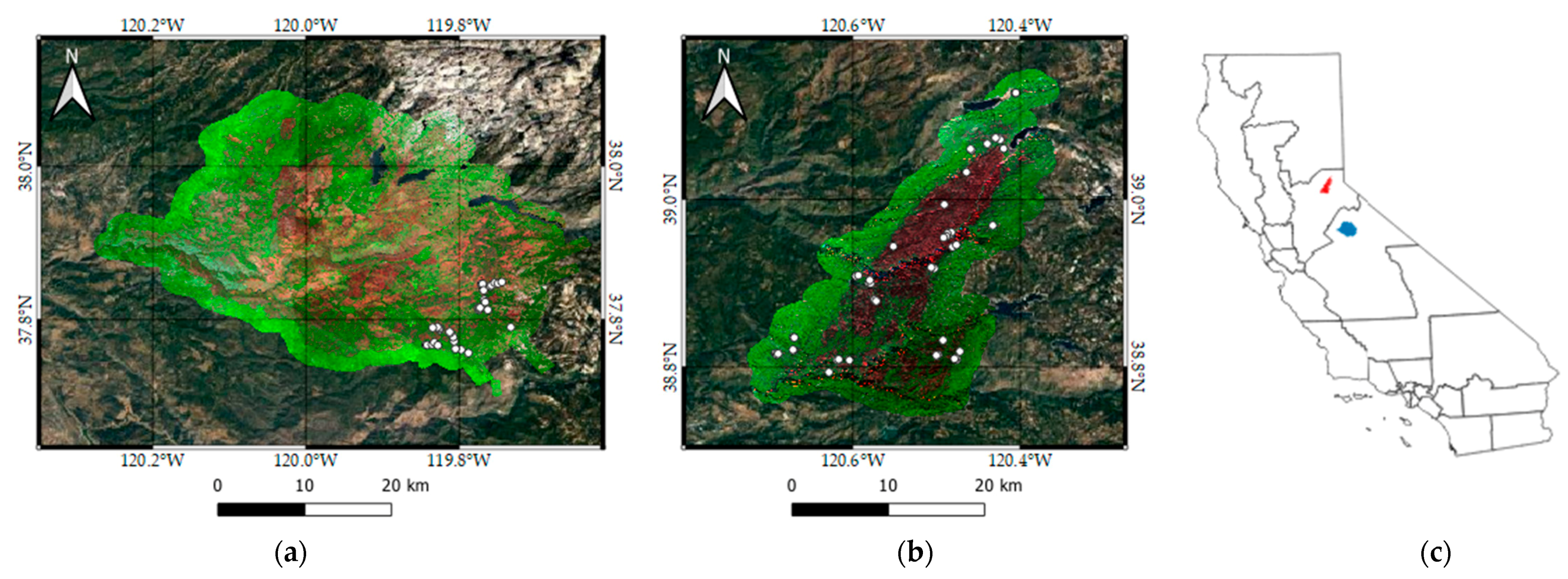
2.1. Study Areas

This study was conducted over the 2013 Rim and 2014 King fires (Figure 1). Both wildfires occurred in California’s Sierra Nevada (Figure 1b). The Rim fire burned roughly 104,000 ha across Yosemite National Park and the Stanislaus National Forest from 17 August 2013 until 24 October 2013 (Figure 1a, Step 1 Figure 2). The King fire burned approximately 40,000 ha from 13 September 2014 until 9 October 2014 in the Eldorado National Forest (Figure 1c, Step 1 Figure 2). Both burned through a mosaic of vegetation dominated by dense mature forests of ponderosa pine (Pinus ponderosa), douglas fir (Pseudotsuga menziesii) and incense cedar (Calocedrus decurrens) [30,31,32]. Both fire locations are topographically complex and are characterized by steep and rugged terrain. Moreover, significant elevation differences are present in both fire scars. The Rim fire scar varied between approximately 600 m and 2400 m, and the King fire scar between 800 m and 1700 m.

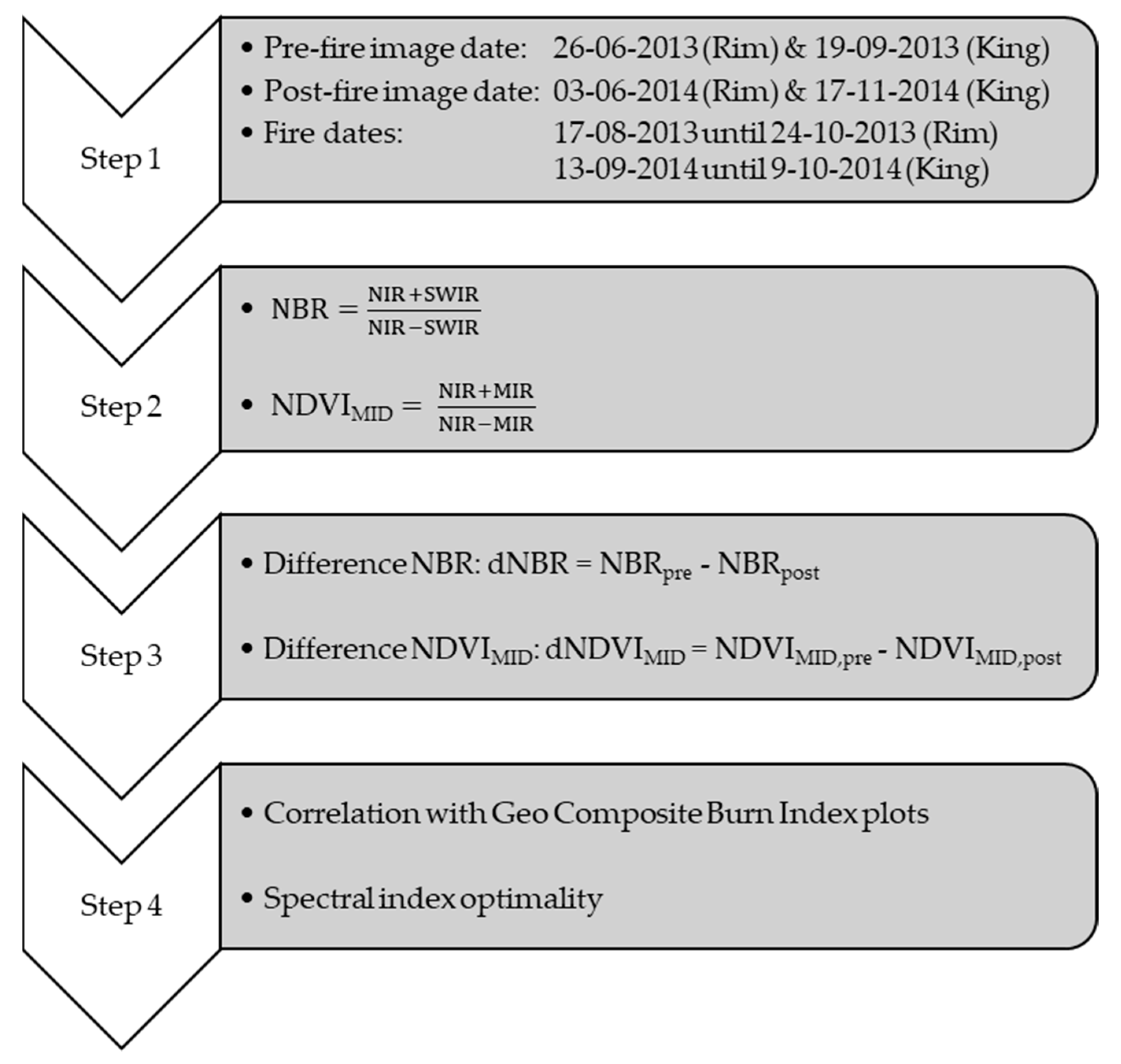
2.2. Airborne Imagery and Processing

There are currently no spaceborne sensors with a MIR band at a spatial resolution of approximately 30 m. This study capitalized upon the unique opportunity stemming from the pre- and post-fire airborne acquisitions over the Rim and King fires with the MASTER instrument. The MASTER scanner acquires data over the spectral range from 0.4 μm to 13 μm in 50 spectral bands. The spatial resolution depends on the flying height and was approximately 35 m over the Rim and King fires [33]. We used Level 2 surface reflectance data in this study. The MASTER bands in the visible to short-wave infrared spectral regions were atmospherically corrected using a radiative transfer model, while surface reflectance in the mid infrared regions was retrieved following Kaufman and Remer [34]. All surface reflectance bands were topographically corrected using the modified c-correction approach [35]. The pre-fire image acquisition covered approximately 97% of the Rim fire perimeter and 92% of the King perimeter with a two km buffer in the two months preceding the fires and the entire perimeter, including buffers, after the fire. For the King fire, however, the MASTER data covered the full fire perimeter with a two km buffer, in both the pre- and post-fire imageries.
The pre- and post-fire image acquisition dates were close to anniversary date acquisitions for both fires and phenological differences between images were thus minimal. In this study, MASTER band 9, centred at 0.87 µm, was used as the NIR band in the spectral index calculations (Step 2 Figure 2). Three suitable MASTER bands covered both the SWIR and MIR spectral ranges. This allowed calculation of three different NBR and NDVIMID indices (Step 2 Figure 2). The MASTER bands 21 (centred on 2.16 µm), 22 (centred on 2.21 µm) and 23 (centred on 2.26 µm) cover the SWIR spectral region. The MASTER bands 28 (centred on 3.61 µm), 29 (centred on 3.76 µm) and 30 (centred on 3.91 µm) cover the MIR spectral region. We thus calculated three different NBR indices. NBR1 was calculated with MASTER band 21 as SWIR band, NBR2 with band 22 and NBR3 with band 23 (Table 1).
Similarly, we calculated three different NDVIMID indices. NDVIMID,1 was calculated with MASTER band 28, NDVIMID,2 with band 29 and NDVIMID,3 with band 30. After this, all indices were bi-temporally differenced by subtracting the post-fire index values from the pre-fire index values (Step 3 Figure 2).

2.3. Relationship with Fire Severity Field Data

Fire severity was assessed in the field using the Geometrically structured Composite Burn Index (GeoCBI) [36] in 33 plots in the Rim fire and 52 plots in the King fire. The GeoCBI is a modified version of the Composite Burn Index (CBI) [36,37]. The main modification of the GeoCBI in comparison with the CBI is that it accounts for the fractional cover of vegetation strata and as such plot-level fire severity is estimated as the weighted average of the fire severity estimates of the different vegetation strata. Both the CBI and GeoCBI have been widely used to validate remotely sensed fire severity assessments [17,20,36,38]. The GeoCBI divides ecosystems into strata and thereby differentiates between one substrate and four vegetation strata. The strata are: (i) substrates; (ii) herbs, low shrubs and small trees shorter than 1 m; (iii) tall shrubs and trees of 1 to 5 m; (iv) intermediate trees of 5 to 20 m; and (v) big trees taller than 20 m (Table 2). For each stratum, several aspects related to fire severity can be rated, when present. Some examples are soil and rock cover and its colour changes, the percentage change in leaf area index, char height and percentage of green vegetation [16,36]. Ratings are based on ocular assessment and scale between zero and three, in which zero represents unburned and three represents high severity. Based on the stratum averages, GeoCBI is calculated in proportion to the corresponding fraction of cover of each stratum, resulting in a weighted average between zero and three that expresses plot-level fire severity (Table 3) [16]. The field plots consisted of 30 m × 30 m squares and were taken in larger areas that were homogeneous with regards to pre-fire vegetation and fire severity. Field plots were sampled in order to represent the observed range of fire severity in mixed conifer forests. The selection of the field plots was constrained by road and trail accessibility, and the centre of the field plot was always at least 100 m away from the nearest road or trail. Field locations were recorded using a Global Navigation Satellite System device.

2.4. Spectral Index Optimality

Spectral index optimality gauges an index’s sensitivity to the change of interest, in this case, fire-induced ecosystem changes and thus fire severity [7,16]. In the case of NDSIs, index optimality is defined by the direction and magnitude of pixel displacements in the bi-spectral space [39]. This can be illustrated by the displacement from unburned U to burned B in the bi-spectral space (Figure 3). Within the bi-spectral space, the y-axis represents the NIR reflectance for all indices, while the x-axis represents the SWIR reflectance for the dNBR indices, and the MIR reflectance for the dNDVIMID indices. The vector |UB| consists of the sum of the vectors |UO| and |OB|. A spectral index is then sensitive to displacements that are perpendicular to the index isolines. In this case, the spectral index is sensitive to the displacement from U to the optimally sensed O. In contrast, the spectral index is insensitive to displacements along isolines, in this case, the vector |OB|. By measuring the distances of the vectors |UO| and |OB|, the index optimality is defined as:
Optimality = 1 − |OB|/|UB|
As |OB| can never exceed |UB|, the optimality varies between zero and one. When the optimality equals zero, then the index is completely insensitive to the change of interest. Whereas an optimality score of one suggests that an index performs ideally in monitoring the change of interest, in this case fire severity. All pixels within the fire perimeter were used in this analysis.

2.5. Analysis

In this present study, a non-linear model based on a saturated growth model was used to describe the relationship between GeoCBI and the NDSIs [40]. The saturated growth model has outperformed linear regression models to describe the relationships between the dNBR and GeoCBI. It accounts for the saturation that occurs with the dNBR for high fire severity plots [40]. The regression results of the saturated growth model were compared using two goodness-of-fit parameters: (i) the coefficient of determination R2 and (ii) the root mean square error (RMSE). The coefficient of determination is an estimate of the proportion of the total variation in the data that is explained by the model. The RMSE is a measure of how much a response variable varies from the model predictions, it is expressed in the same units as the dependent dataset. In addition, optimality statistics of all burned pixels were compared for the different indices, and thus excluding the two km buffer zone around the fire perimeter. The median statistic was used for this purpose due to its robustness in identifying outliers and the non-normal optimality distributions.

3. Results

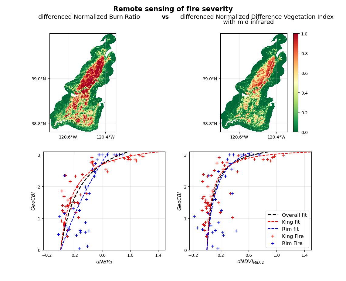
3.1. Relationships between Field and Airborne Data
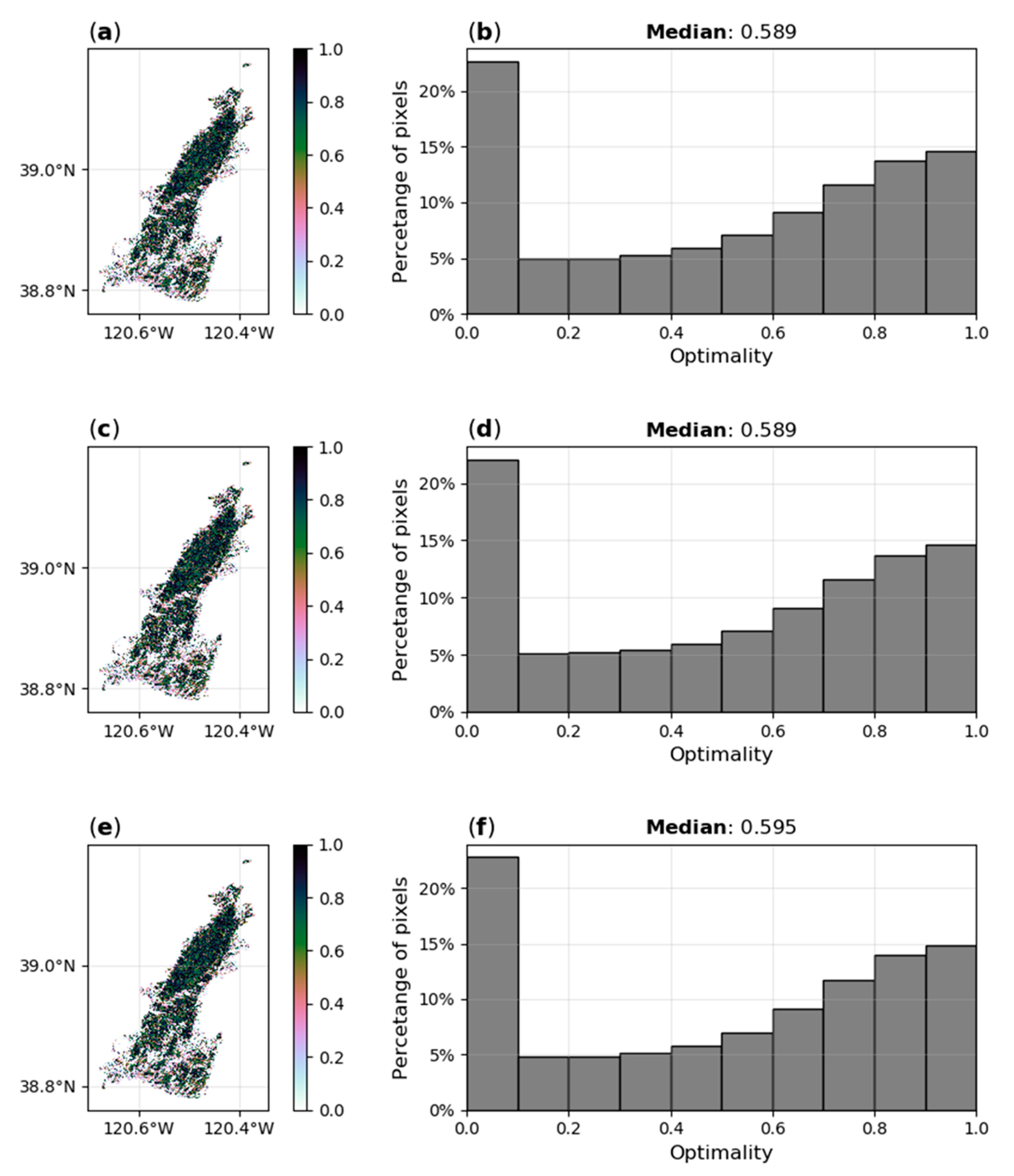
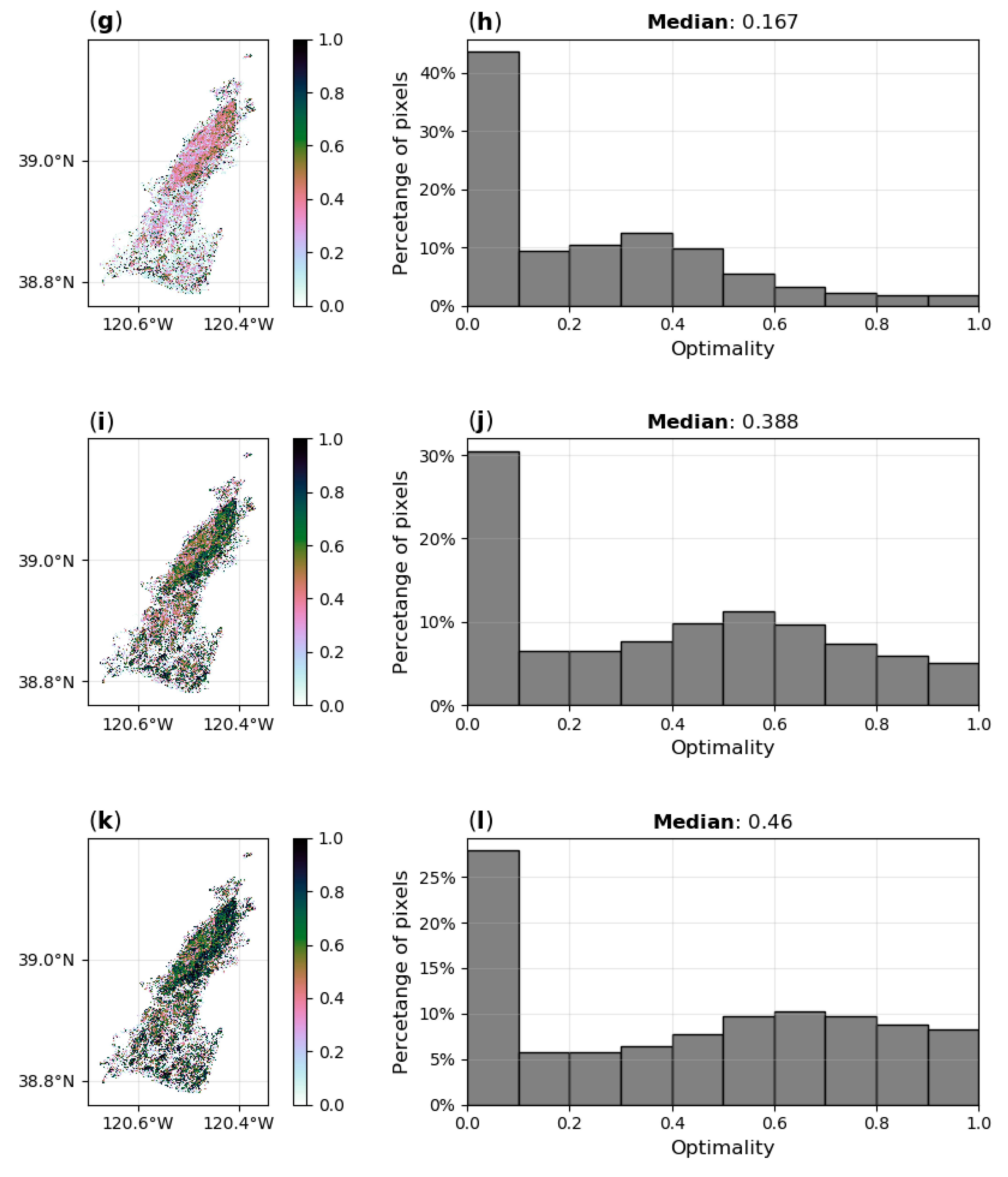
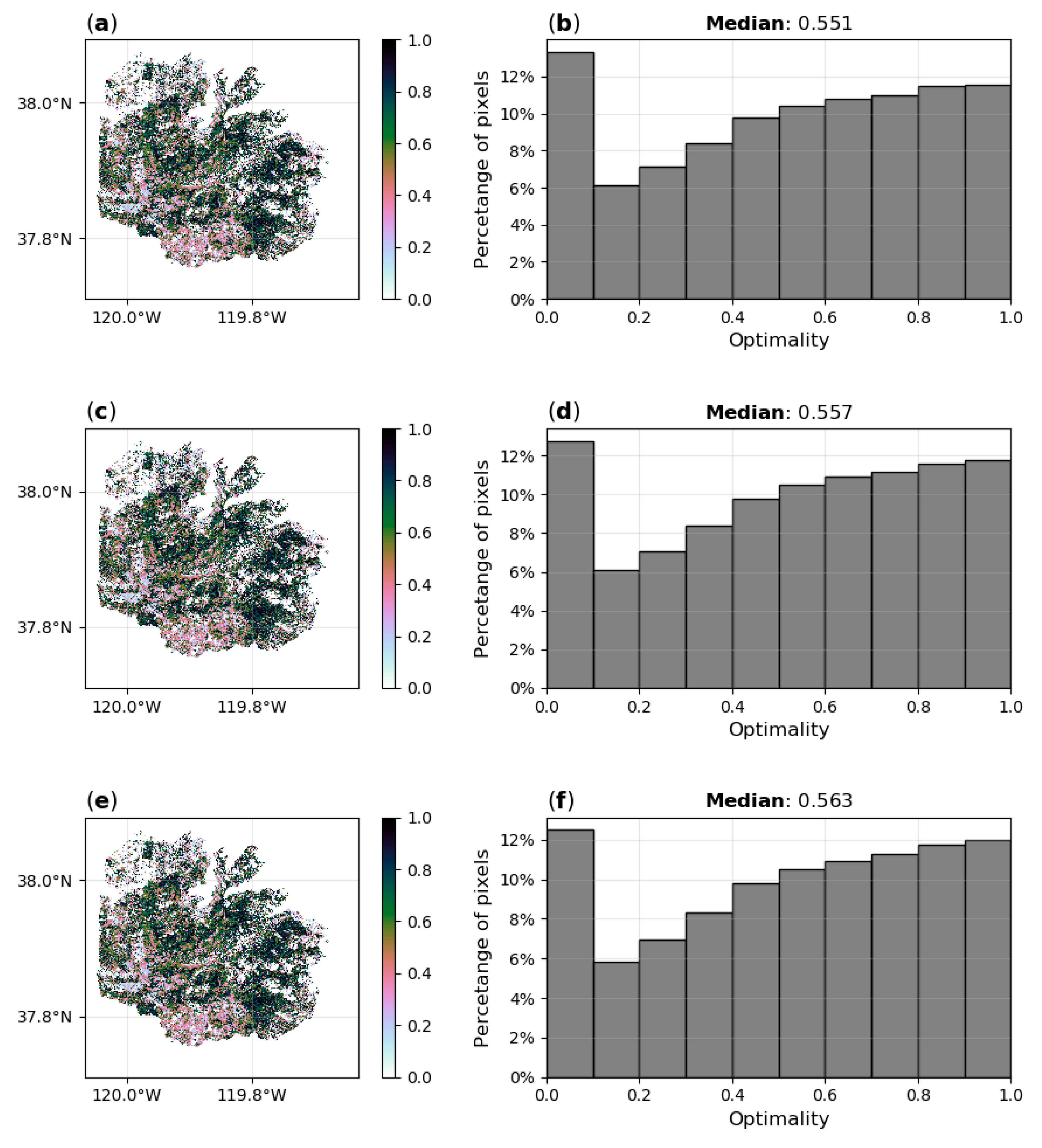
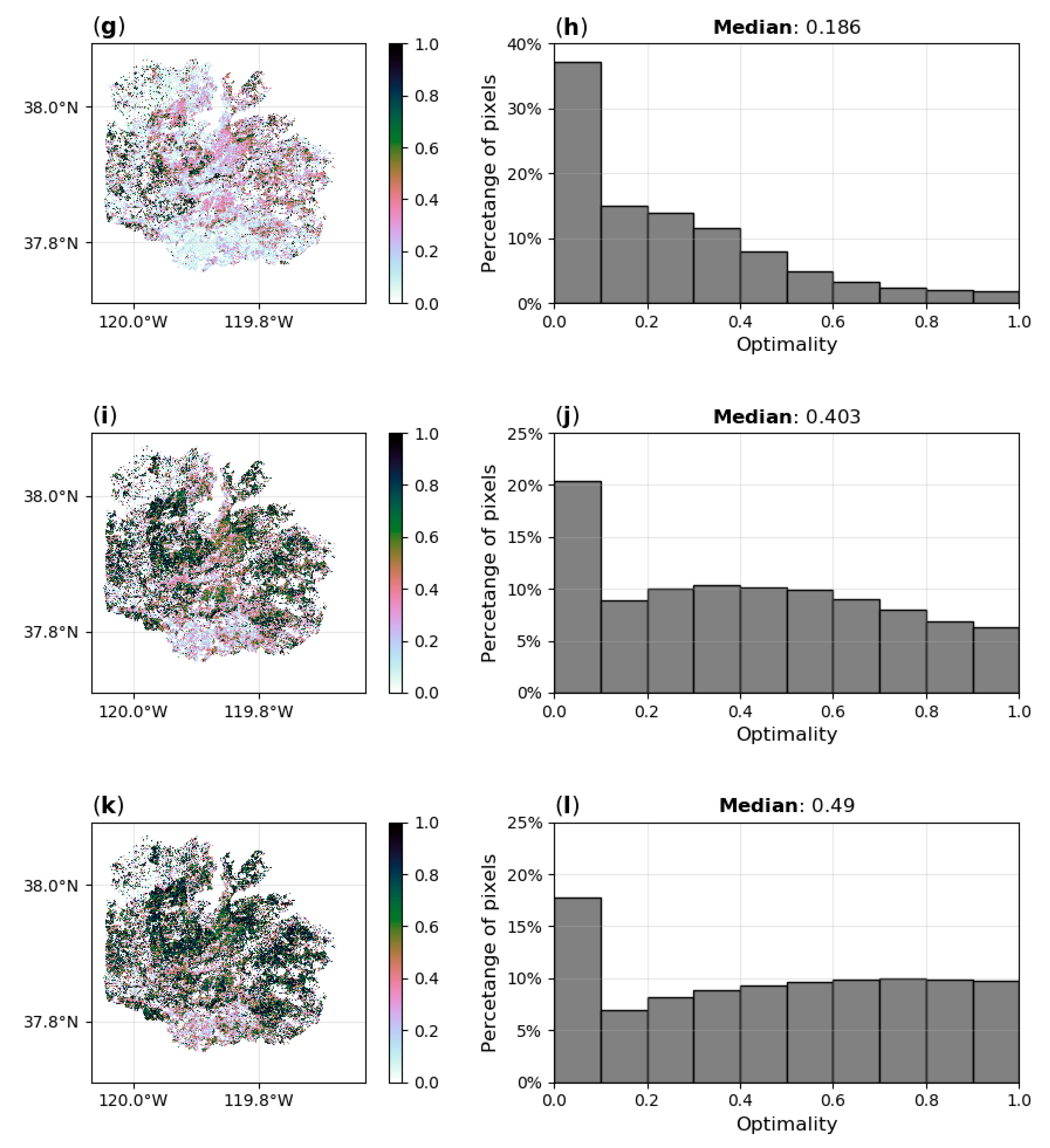
The indices were bi-temporally differenced by subtracting the post-fire index values from the pre-fire index values (Step 3 Figure 2). These differenced maps are shown in Figure 4. All spectral indices demonstrated reasonably strong relationships with the GeoCBI (Figure 5a–f). For the pooled dataset over the two fires, all dNBR indices performed better than the dNDVIMID indices. The dNBR3 index demonstrated the best performance yielding an R2 of 0.68. For the dNBR indices, the relationship with field data was stronger and different across the Rim and King fire (Table 4). This difference in the form of the regression line is less pronounced in the relationships between the two fires for the dNDVIMID indices (Figure 5d–f). For those indices, regression lines of the individual fire events are very close to each other.
For the individual NDSIs, different RMSE trends can be observed between these fires. The decreasing trend in R2 statistic of the Rim fire is associated with an increasing RMSE. For the King fire, this decreasing trend results in a decrease in RMSE. The spectral index values of the dNDVIMID,3 displayed the largest value range. The ranges of values were more variable among the dNDVIMID indices compared to the dNBR indices, with the largest range corresponding the dNDVIMID index that was constructed with MIR band centred at 3.91 µm (Figure 5f).

3.2. Optimality

The optimality of the dNBR indices was always higher than from the dNDVIMID indices, with only small differences between the different dNBR indices (Figure 6 and Figure 7). All three dNBR indices have similar optimality statistics; however, the highest median optimality for both fires was observed for the dNBR3. The median optimality of the dNBR3 was 0.60 over the King fire and 0.56 over the Rim fires. The optimality of the dNDVIMID varied widely between the indices. The highest optimality of the dNDVIMID indices was obtained by the dNDVIMID,3 index, with a median optimality of 0.46 in the King fire, and 0.49 in the Rim fire. In all indices, a large percentile of pixels recorded an optimality value lower than 0.1. This may be because unburned pixels patches may be included in the mapped fire perimeter. Across both fires, the optimality of the dNBR indices with optimality values higher than 0.1 showed a trend towards more pixels with higher optimality values. This trend was absent in the optimality distributions of the dNDVIMID indices. While median optimality values demonstrated small differences between both fires, the relative optimality performance of the indices was the same for both fires.

4. Discussion

The overall results of the pooled dataset showed a moderately high correlation between GeoCBI field data and the proposed NDSIs for a temperate environment, such as California (USA). The dNBR indices performed better than the dNDVIMID indices. These model outcomes fall within the ranges observed within previous GeoCBI-dNBR relationships studies [16,23,41]. Large residual variability among each fitted model indicated relatively high uncertainties in the predictability of fire severity (Figure 5). Similar asymptotic behaviour is exhibited across all NDSIs in relation to the moderate to high GeoCBI values. The inability and underestimation of the dNBR indices to distinguish among high severity sites highlighted in previous GeoCBI-dNBR models have been the driver of attempting non-linear asymptotic modelling as suggested by Hall [20,40]. In our study, similar saturation of spectral indices for high severity plots occurred justifying the use of a saturated growth model [16]. Previous studies based on the spectral index theory, reported that the dNBR outperformed other dNDSI with regards to optimality distributions [6,16]. In these studies, the dNBR outperformed the differenced NDVI (dNDVI) and differenced normalized difference moisture index (dNDMI). Our dNBR results approximated earlier reported values for the dNBR and fall within ranges recorded in six Alaskan fires by Murphy et al. [41].
In addition, our results reaffirm the strength of the dNBR as being the most sensitive to fire-induced changes in spectral reflectance, and less so to noise. Over both fire scars, the dNBR’s optimality was consistently higher than what was observed for the dNDVIMID. The optimality statistics for the dNDVIMID resulted in a large variety of mean values ranging from 0.167 to 0.46. Roy et al. [7] conducted an optimality analysis on the dNBR of MODIS-sensed fires in the boreal forest in Russia, African savannas and the South American tropical forest. Roy et al. [7] included both unburned and burned pixels in their analysis, and roughly a third of their analysed pixels had optimality scores lower than 0.1. Including unburned pixels resulted in lower mean optimality scores (between 0.24 and 0.33) than in studies which excluded the unburned pixels [6,7,16]. Our analysis reports a similar percentage of pixels with an optimality score lower than 0.1. These pixels may be unburned patches that were included in the fire perimeter.
Studies assessing the correlation between several spectral indices and GeoCBI or CBI field data identified the NBR as the best index in the bi-temporal differencing approach [16,22]. Moreover, this study confirms that the dNBR outperforms the dNDVIMID. Despite this relative success, our analyses confirm the same large variability in the form of relationships across fires as mentioned by previous studies [22,40,41]. This variability may partly be caused by the spectral sensitivity of the SWIR spectral region to soil variations [5,7]. The dNBR approach is therefore most likely affected by variability in background conditions. This hampers comparison of dNBR across fires with different soil conditions. Miller and Thode [42] have proposed the relative dNBR (RdNBR) in which the dNBR is divided by the square root of the pre-fire NBR. The RdNBR as such accounts for differences in pre-fire vegetation cover and enhances the intercomparison over heterogeneous landscapes. The dNDVIMID indices displayed a reduced variability in regression forms across the Rim and King fires. This improved intercomparison across different fires from the dNDVIMID is in line with previously reported improvements in discriminating between unburned and burned pixels [26,43]. This suggests that the dNDVIMID bi-temporal differencing approach may result in a more comparable fire severity proxy over large regions.
Based on the dNDVIMID pooled data-GeoCBI correlations, the indices that were constructed with MIR band centred at 3.76 µm (dNDVIMID,2) and 3.91 µm (dNDVIMID,3) provided similar results regarding their coefficients of determinations (R2 = 0.61) and outperformed the index centred at 3.61 µm (dNDVIMID,1). The GeoCBI–dNDVIMID,2 model yielded the lowest RMSE of 0.48, which is approximately one-sixth of the total GeoCBI variation (Table 3). The NDVIMID,2 also demonstrated the smallest variation in regression from across the two fires (Figure 5d). Furthermore, the dNDVIMID,2 also displayed a wider spectral range for the 85 samples than the dNBR indices. This holds also true for the dNDVIMID,3. This first spectral optimality analysis of the dNDVIMID displayed large variation in performance dependent on the wavelengths used for the MIR bands. The dNDVIMID index that integrated the MIR band with the longest wavelength yielded the highest optimality scores, in which the dNDVIMID,3 index approached an optimality of 0.5.
Potential sources of inaccuracy in our analysis arise from both the field and satellite observations. To fulfil the need for a stratified sampling approach of the GeoCBI, it is required that the number of plots for each fuel type are in proportion to the total area burned of each fuel type. Because of accessibility limitations, we were unable to fulfil these conditions. Part of the observed divergence between field and remotely sensed fire severity estimates can also be explained by the fact that both field and satellite data are imperfect proxies of fire severity. The GeoCBI is based on a semi-quantitative judgement approach, which is inherently prone to some degree of subjectivity, especially when different people perform the field assessments. This was the case in our study in which different field teams surveyed the Rim and King fires. Several noise factors can impede remote sensing image analyses. The amount of noise in all spectral indices was substantial, as the median optimality scores are considerably lower than the optimal score of one. Noise within remote sensing analysis can result from imperfections in image pre-processing and slight deviations in phenology between near-anniversary date image acquisitions. Garcia et al. [44] recently developed a new metric, the waveform area relative change (WARC), from light detection and ranging (LiDAR) imagery. The WARC proxy captures changes in vegetation structure as well as changes in soil and leaf colour and was successfully validated over the King fire. Synergistic use of such LiDAR derived metrics with optical indices like the dNBR and dNDVIMID could provide insights on how differences in vegetation structure influence the performance of spectral indices. Our findings can contribute to improvements in the remote sensing of fire severity, as it proposes an index with similar performance as the current dNBR approach. Our preliminary findings of the dNDVIMID approach suggest that use of the dNDVIMID index for fire severity assessment may lead to more comparable remote sensing assessments among fire scars than with the dNBR. We evaluated the dNDVIMID thanks to the unique availability of pre- and- post-fire MASTER imagery over the Rim and King fires. The potential of the dNDVIMID for assessing fire severity needs further evaluation when consistent MIR imagery acquisition will become available at a spatial resolution of less than 100 m, allowing comparison with field measurements of fire severity.

5. Conclusions

The results of our comparison between field and remotely sensed proxies of fire severity and the spectral optimality analysis confirmed the dNBR as a strong fire severity predictor. Overall, the dNBR yielded better results than the dNDVIMID in estimating fire severity over two Californian fires. The field data analysis, however, also identified that the dNBR approach suffered from significant variations in the form of regression lines across the two fires. The saturated growth fit between field and dNDVIMID data resulted in more comparable regression lines across the two fires, despite a slightly lower overall performance than the dNBR. This suggests the dNDVIMID bi-temporal differencing approach may be a more robust method in estimating and comparing fire severity over large regions. Our study leveraged unique pre- and post-fire airborne acquisitions over the Rim and King fires in California from the MASTER sensor. As such, our study is the first to assess the NIR–MIR bi-spectral space for assessing fire severity and calls for a continued evaluation of dNDVIMID for assessing fire severity. This will require pre- and post-fire imagery to be available for the MIR spectral region at a spatial resolution that allows comparison with field measurements.

Author Contributions

This article is part of a master’s research project written by M.J.v.G. at VU Amsterdam. S.V. designed and supervised the project. S.V. acquired field measurements. M.J.v.G. performed the analyses with input from S.V. M.J.v.G. and S.V. wrote the manuscript. All authors have read and agreed to the published version of the manuscript.

Funding

This research did not receive funding.

Institutional Review Board Statement

Not applicable.

Informed Consent Statement

Not applicable.

Data Availability Statement

In our study we used pre-processed data by the Jet Propulsion Laboratory. This is public available data and can be found at: https://wildfire.jpl.nasa.gov/data/ (accessed on 20 January 2021).

Acknowledgments

We would like to thank and acknowledge the Jet Propulsion Laboratory for the pre-processing of the spectral bands used in this article. We thank Simon Hook and Linley Kroll for supporting the field data collection in the Rim fire, and Natasha Stavros for sharing field data collected in the King fire. We are also thankful to the personnel of Yosemite National Park, the Stanislaus National Forest and Eldorado National Forest for permissions to conduct field work.

Conflicts of Interest

The authors declare no conflict of interest.

References

  1. Barbero, R.; Abatzoglou, J.T.; Larkin, N.K.; Kolden, C.A.; Stocks, B. Climate change presents increased potential for very large fires in the contiguous United States. Int. J. Wildl. Fire 2015, 24, 892–899. [Google Scholar] [CrossRef]
  2. Dennison, P.E.; Brewer, S.C.; Arnold, J.D.; Moritz, M.A. Large wildfire trends in the western United States, 1984–2011. Geophys. Res. Lett. 2014, 41, 2928–2933. [Google Scholar] [CrossRef]
  3. Westerling, A.L.R. Increasing western US forest wildfire activity: Sensitivity to changes in the timing of spring. Philos. Trans. R. Soc. B Biol. Sci. 2016, 371. [Google Scholar] [CrossRef]
  4. Stavros, E.N.; Abatzoglou, J.T.; McKenzie, D.; Larkin, N.K. Regional projections of the likelihood of very large wildland fires under a changing climate in the contiguous Western United States. Clim. Chang. 2014, 126, 455–468. [Google Scholar] [CrossRef]
  5. Smith, A.M.S.; Eitel, J.U.H.; Hudak, A.T. Spectral analysis of charcoal on soils implications. Int. J. Wildl. Fire 2010, 19, 976–983. [Google Scholar] [CrossRef]
  6. Escuin, S.; Navarro, R.; Fernández, P. Fire severity assessment by using NBR (Normalized Burn Ratio) and NDVI (Normalized Difference Vegetation Index) derived from LANDSAT TM/ETM images. Int. J. Remote Sens. 2008, 29, 1053–1073. [Google Scholar] [CrossRef]
  7. Roy, D.P.; Boschetti, L.; Trigg, S.N. Remote sensing of fire severity: Assessing the performance of the normalized burn ratio. IEEE Geosci. Remote Sens. Lett. 2006, 3, 112–116. [Google Scholar] [CrossRef] [Green Version]
  8. Keeley, J.E. Fire intensity, fire severity and burn severity: A brief review and suggested usage. Int. J. Wildl. Fire 2009, 18, 116–126. [Google Scholar] [CrossRef]
  9. Hammill, K.A.; Bradstock, R.A. Remote sensing of fire severity in the Blue Mountains: Influence of vegetation type and inferring fire intensity. Int. J. Wildl. Fire 2006, 15, 213–226. [Google Scholar] [CrossRef]
  10. Chafer, C.J. A comparison of fire severity measures: An Australian example and implications for predicting major areas of soil erosion. Catena 2008, 74, 235–245. [Google Scholar] [CrossRef]
  11. Chafer, C.J.; Noonan, M.; Macnaught, E. The post-fire measurement of fire severity and intensity in the Christmas 2001 Sydney wildfires. Int. J. Wildl. Fire 2004, 13, 227–240. [Google Scholar] [CrossRef]
  12. González-Alonso, F.; Merino-De-Miguel, S.; Roldán-Zamarrón, A.; García-Gigorro, S.; Cuevas, J.M. MERIS full resolution data for mapping level-of-damage caused by forest fires: The Valencia de Alcántara event in August 2003. Int. J. Remote Sens. 2007, 28, 797–809. [Google Scholar] [CrossRef]
  13. Brewer, C.K.; Winne, J.C.; Redmond, R.L.; Opitz, D.W.; Mangrich, M. Classifying and Mapping Wildfire Severity: A Comparison of Methods. Photogramm. Eng. Remote Sens. 2005, 71, 1311–1320. [Google Scholar] [CrossRef] [Green Version]
  14. Jain, T.B. Tongue-Tied: Confused meanings for common fire terminology can lead to fuels mismanagement. Wildfire 2004, 22–26. [Google Scholar]
  15. Lentile, L.B.; Holden, Z.A.; Smith, A.M.S.; Falkowski, M.J.; Hudak, A.T.; Morgan, P.; Lewis, S.A.; Gessler, P.E.; Benson, N.C. Remote sensing techniques to assess active fire characteristics and post-fire effects. Int. J. Wildl. Fire 2006, 15, 319–345. [Google Scholar] [CrossRef]
  16. Veraverbeke, S.; Verstraeten, W.W.; Lhermitte, S.; Goossens, R. Evaluating Landsat Thematic Mapper spectral indices for estimating burn severity of the 2007 Peloponnese wildfires in Greece. Int. J. Wildl. Fire 2010, 19, 558–569. [Google Scholar] [CrossRef] [Green Version]
  17. Key, C.H. Remote sensing sensitivity to fire severity and fire recovery. In Proceedings of the 5th International Workshop on Remote Sensing and GIS Applications to Forest Fire Management: Fire Effects Assessment, Zaragoza, Spain, 16–18 June 2005; pp. 29–39. [Google Scholar]
  18. Jakubauskas, M.E.; Lulla, K.P.; Mausel, P.W. Assessment of vegetation change in a fire-altered forest landscape. PE&RS Photogramm. Eng. Remote Sens. 1990, 56, 371–377. [Google Scholar]
  19. Cocke, A.E.; Fulé, P.Z.; Crouse, J.E. Comparison of burn severity assessments using Differenced Normalized Burn Ratio and ground data. Int. J. Wildl. Fire 2005, 14, 189–198. [Google Scholar] [CrossRef] [Green Version]
  20. Van Wagtendonk, J.W.; Root, R.R.; Key, C.H. Comparison of AVIRIS and Landsat ETM+ detection capabilities for burn severity. Remote Sens. Environ. 2004, 92, 397–408. [Google Scholar] [CrossRef]
  21. García, M.J.L.; Caselles, V. Mapping burns and natural reforestation using thematic mapper data. Geocarto Int. 1991, 6, 31–37. [Google Scholar] [CrossRef]
  22. Epting, J.; Verbyla, D.; Sorbel, B. Evaluation of remotely sensed indices for assessing burn severity in interior Alaska using Landsat TM and ETM+. Remote Sens. Environ. 2005, 96, 328–339. [Google Scholar] [CrossRef]
  23. French, N.H.F.; Kasischke, E.S.; Hall, R.J.; Murphy, K.A.; Verbyla, D.L.; Hoy, E.E.; Allen, J.L. Using Landsat data to assess fire and burn severity in the North American boreal forest region: An overview and summary of results. Int. J. Wildl. Fire 2008, 17, 443–462. [Google Scholar] [CrossRef]
  24. De Santis, A.; Chuvieco, E. Burn severity estimation from remotely sensed data: Performance of simulation versus empirical models. Remote Sens. Environ. 2007, 108, 422–435. [Google Scholar] [CrossRef]
  25. Libonati, R.; DaCamara, C.C.; Pereira, J.M.C.; Peres, L.F. Retrieving middle-infrared reflectance for burned area mapping in tropical environments using MODIS. Remote Sens. Environ. 2010, 114, 831–843. [Google Scholar] [CrossRef]
  26. Libonati, R.; DaCamara, C.C.; Pereira, J.M.C.; Peres, L.F. Retrieving middle-infrared reflectance using physical and empirical approaches: Implications for burned area monitoring. IEEE Trans. Geosci. Remote Sens. 2012, 50, 281–294. [Google Scholar] [CrossRef]
  27. Libonati, R.; DaCamara, C.C.; Pereira, J.M.C.; Peres, L.F. On a new coordinate system for improved discrimination of vegetation and burned areas using MIR/NIR information. Remote Sens. Environ. 2011, 115, 1464–1477. [Google Scholar] [CrossRef]
  28. Eck, T.F.; Holben, B.N.; Slutsker, I.; Setzer, A. Measurements of irradiance attenuation and estimation of aerosol single scattering albedo for biomass burning aerosols in Amazonia. J. Geophys. Res. Atmos. 1998, 103, 31865–31878. [Google Scholar] [CrossRef]
  29. Pereira, J.M.C. A comparative evaluation of NOAA/AVHRR vegetation indexes for burned surface detection and mapping. IEEE Trans. Geosci. Remote Sens. 1999, 37, 217–226. [Google Scholar] [CrossRef]
  30. Casas, Á.; García, M.; Siegel, R.B.; Koltunov, A.; Ramírez, C.; Ustin, S. Burned forest characterization at single-tree level with airborne laser scanning for assessing wildlife habitat. Remote Sens. Environ. 2016, 175, 231–241. [Google Scholar] [CrossRef] [Green Version]
  31. Stavros, E.N.; Coen, J.; Peterson, B.; Singh, H.; Kennedy, K.; Ramirez, C.; Schimel, D. Use of imaging spectroscopy and LIDAR to characterize fuels for fire behavior prediction. Remote Sens. Appl. Soc. Environ. 2018, 11, 41–50. [Google Scholar] [CrossRef]
  32. Tane, Z.; Roberts, D.; Veraverbeke, S.; Casas, Á.; Ramirez, C.; Ustin, S. Evaluating endmember and band selection techniques for multiple endmember spectral mixture analysis using post-fire imaging spectroscopy. Remote Sens. 2018, 10, 389. [Google Scholar] [CrossRef] [Green Version]
  33. Stavros, E.N.; Tane, Z.; Kane, V.R.; Veraverbeke, S.; McGaughey, R.J.; Lutz, J.A.; Ramirez, C.; Schimel, D. Unprecedented remote sensing data over King and Rim megafires in the Sierra Nevada Mountains of California. Ecology 2016, 97, 3244. [Google Scholar] [CrossRef]
  34. Kaufman, Y.J.; Remer, L.A. Detection of forests using mid-IR reflectance: An application for aerosol studies. IEEE Trans. Geosci. Remote Sens. 1994, 32, 672–683. [Google Scholar] [CrossRef]
  35. Veraverbeke, S.; Verstraeten, W.W.; Lhermitte, S.; Goossens, R. Illumination effects on the differenced Normalized Burn Ratio’s optimality for assessing fire severity. Int. J. Appl. Earth Obs. Geoinf. 2010, 12, 60–70. [Google Scholar] [CrossRef] [Green Version]
  36. De Santis, A.; Chuvieco, E. GeoCBI: A modified version of the Composite Burn Index for the initial assessment of the short-term burn severity from remotely sensed data. Remote Sens. Environ. 2009, 113, 554–562. [Google Scholar] [CrossRef]
  37. Key, C.H.; Benson, N.C. Landscape Assessment (LA) Sampling and Analysis Methods. Available online: https://www.fs.usda.gov/treesearch/pubs/24066 (accessed on 20 January 2021).
  38. Veraverbeke, S.; Stavros, E.N.; Hook, S.J. Assessing fire severity using imaging spectroscopy data from the Airborne Visible/Infrared Imaging Spectrometer (AVIRIS) and comparison with multispectral capabilities. Remote Sens. Environ. 2014, 154, 153–163. [Google Scholar] [CrossRef]
  39. Verstraete, M.M.; Pinty, B. Designing optimal spectral indexes for remote sensing applications. IEEE Trans. Geosci. Remote Sens. 1996, 34, 1254–1265. [Google Scholar] [CrossRef]
  40. Hall, R.J.; Freeburn, J.T.; De Groot, W.J.; Pritchard, J.M.; Lynham, T.J.; Landry, R. Remote sensing of burn severity: Experience from western Canada boreal fires. Int. J. Wildl. Fire 2008, 17, 476–489. [Google Scholar] [CrossRef]
  41. Murphy, K.A.; Reynolds, J.H.; Koltun, J.M. Evaluating the ability of the differenced Normalized Burn Ratio (dNBR) to predict ecologically significant burn severity in Alaskan boreal forests. Int. J. Wildl. Fire 2008, 17, 490–499. [Google Scholar] [CrossRef]
  42. Miller, J.D.; Thode, A.E. Quantifying burn severity in a heterogeneous landscape with a relative version of the delta Normalized Burn Ratio (dNBR). Remote Sens. Environ. 2007, 109, 66–80. [Google Scholar] [CrossRef]
  43. Veraverbeke, S.; Hook, S.J.; Harris, S. Synergy of VSWIR (0.4–2.5 μm) and MTIR (3.5–12.5 μm) data for post-fire assessments. Remote Sens. Environ. 2012, 124, 771–779. [Google Scholar] [CrossRef]
  44. García, M.; North, P.; Viana-Soto, A.; Stavros, N.E.; Rosette, J.; Martín, M.P.; Franquesa, M.; González-Cascón, R.; Riaño, D.; Becerra, J.; et al. Evaluating the potential of LiDAR data for fire damage assessment: A radiative transfer model approach. Remote Sens. Environ. 2020, 247. [Google Scholar] [CrossRef]
Figure 1. Infrared colour composites of the study areas, in which Red: MASTER band 21 (centred at 2.16 µm), Green: MASTER band 9 (centred at 0.87 µm), and Blue: MASTER band 5 (centred at 0.66 µm). (a) Shows the extent of the Rimfire; (b) Shows the extent of the King fire; (c) Shows an overview map of California USA, visualizing the Rim fire (blue) and the King fire (red). In both (a,b), the white circles represent the field sampling locations. Background images display Google Earth imagery.
Remotesensing 13 00695 g001
Figure 2. Methodological workflow.
Remotesensing 13 00695 g002
Figure 3. Example of pre- and post-fire trajectory of a pixel in the NIR–SWIR and NIR–MIR bi-spectral space. A pixel displaces from unburned (U) to burned (B). O resembles the position of an optimally sensed burned pixel. (NIR: near infrared, SWIR: short-wave infrared, MIR: mid infrared).
Remotesensing 13 00695 g003
Figure 4. Pre- and post-fire differenced maps of both the King (af) and Rim (gl). The colour display visualizes the differenced value of each pixel, the darker the red colours denote pixels with high fire severity values, green colours represent unaffected unburned pixels. (a) dNBR1 King fire; (b) dNBR2 King fire; (c) dNBR3 King fire; (d) dNDVIMID,1 King fire; (e) dNDVIMID,2 King fire; (f) dNDVIMID,3 King fire; (g) dNBR1 Rim fire; (h) dNBR2 Rim fire; (i) dNBR3 Rim fire; (j) dNDVIMID,1 Rim fire; (k) dNDVIMID,2 Rim fire; (l) dNDVIMID,3 Rim fire.
Remotesensing 13 00695 g004aRemotesensing 13 00695 g004b
Figure 5. Scatter plots of GeoCBI field data from the Rim fire (blue) and King fire (red) with multiple regression lines corresponding to the overall data set (black), Rim fire (blue) and King fire (red). (a) GeoCBI-dNBR1; (b) GeoCBI-dNBR2; (c) GeoCBI-dNBR3; (d) GeoCBI-dNDVIMID,1; (e) GeoCBI-dNDVIMID,2; (f) GeoCBI-dNDVIMID,3.
Remotesensing 13 00695 g005
Figure 6. Optimality maps and histograms of the differenced normalized burn ratio (dNBR) indices for the King fire. (a) Optimality map dNBR1; (b) Optimality map dNBR2; (c) Optimality map dNBR3; (d) Histogram of the dNBR1; (e) Histo-gram of the dNBR2; (f) Histogram of the dNBR3. Optimality maps and histograms of the differenced normalized difference vegetation index with mid infrared (dNDVIMID) indices for the King fire. (g) Optimality map dNDVIMID,1; (h) Optimality map dNDVIMID,2; (i) Optimality map dNDVIMID,3; (j) Histogram of the dNDVIMID,1; (k) Histogram of the dNDVIMID,2; (l) Histogram of the dNDVIMID,3.
Remotesensing 13 00695 g006aRemotesensing 13 00695 g006b
Figure 7. Optimality maps and histograms of the differenced normalized burn ratio (dNBR) indices for the Rim fire. (a) Optimality map dNBR1; (b) Optimality map dNBR2; (c) Optimality map dNBR3; (d) Histogram of the dNBR1; (e) Histo-gram of the dNBR2; (f) Histogram of the dNBR3. Optimality maps and histograms of the differenced normalized difference vegetation index with mid infrared (dNDVIMID) indices for the Rim fire. (g) Optimality map dNDVIMID,1; (h) Optimality map dNDVIMID,2; (i) Optimality map dNDVIMID,3; (j) Histogram of the dNDVIMID,1; (k) Histogram of the dNDVIMID,2; (l) Histogram of the dNDVIMID,3.
Remotesensing 13 00695 g007aRemotesensing 13 00695 g007b
Table 1. Spectral indices used in this study. The MASTER band 9, centred on 0.87 µm, was used as the NIR band in the spectral index calculations The MASTER bands 21 (centred on 2.16 µm), 22 (centred on 2.21 µm) and 23 (centred on 2.26 µm) cover the SWIR spectral region. The MASTER bands 28 (centred on 3.61 µm), 29 (centred on 3.76 µm) and 30 (centred on 3.91 µm) cover the MIR spectral region.
NDSIsPre- and Post-Fire Differences
NBR1 = (Band 9 + Band 21)/(Band 9 − Band 21),(1a)dNBR1 = NBR1,pre − NBR1,post,(1b)
NBR2 = (Band 9 + Band 22)/(Band 9 − Band 22),(2a)dNBR2 = NBR2,pre − NBR2,post,(2b)
NBR3 = (Band 9 + Band 23)/(Band 9 − Band 23),(3a)dNBR3 = NBR3,pre − NBR3,post,(3b)
NDVIMID,1 = (Band 9 + Band 28)/(Band 9 − Band 28),(4a)dNDVIMID,1 = NDVIMID,1,pre − NDVIMID,1,post,(4b)
NDVIMID,2 = (Band 9 + Band 29)/(Band 9 − Band 29),(5a)dNDVIMID,2 = NDVIMID,2,pre − NDVIMID,2,post,(5b)
NDVIMID,3 = (Band 9 + Band 30)/(Band 9 − Band 30),(6a)dNDVIMID,3 = NDVIMID,3,pre − NDVIMID,3,post(6b)
NDSI = normalized difference spectral index; NBR = normalized burn ratio; NDVIMID = normalized differenced vegetation index with mid infrared.
Table 2. The Geometrically structured Composite Burn Index (GeoCBI) criteria used to estimate the field fire severity [36].
SchemeFire Severity Scale
No EffectLow EffectModerate EffectHigh Effect
00.51.01.52.02.53.0
Substrates FCOV FCOV
 Litter (l) or light fuel (lf) consumed0%-50% (l)-100% (l)>80% (lf)98% (lf)
 Duff0%-Light char-50%-Consumed
 Medium or heavy fuel0%-20%-40%->60%
 Soil and rock cover–colour0%-10%-40%->80%
Herbs, low shrubs and trees less than 1 m FCOV FCOV
 Percentage foliage altered0%-30%-80%95%100%
 Frequency percentage living100%-90%-50%<20%0%
 New sproutsAbundant-Moderate-high-Moderate-Low-none
Tall shrubs and trees 1 to 5 m FCOV FCOV
 Percentage foliage altered0%-20%-60–90%>95%Branch loss
 Frequency percentage living100%-90%-30%<15%<1%
 LAI change percentage0%-15%-70%90%100%
Intermediate trees 5 to 20 m FCOV FCOV
 Percentage green (unaltered)100%-80%-40%<10%None
 Percentage black or brown0%-20%-60–90%>95%Branch loss
 Frequency percentage living100%-90%-30%<15%<1%
 LAI change percentage0%-15%-70%90%100%
 Char heightNone-1.5 m-2.8 m->5 m
Big trees 4 to 20 m FCOV FCOV
 Percentage green (unaltered)100%-80%-50%<10%None
 Percentage black or brown0%-20%-60–90%>95%Branch loss
 Frequency percentage living100%-90%-30%<15%<1%
 LAI change percentage0%-15%-70%90%100%
 Char heightNone-1.8 m-4 m->7 m
FCOV = fraction of cover; LAI = leaf area index.
Table 3. Photo examples of high, moderate and low fire severity plots in the Rim fire.
Sample PlotDescription
Remotesensing 13 00695 i001High fire severity
GeoCBI rating: 3.00

Large portions of downed fuels are consumed. Substantial soil exposure and soil colour change. Shrubs are absent and only few resprouts are present. The overstorey is mostly consumed, some brown needles have remained.
Remotesensing 13 00695 i002Moderate fire severity
GeoCBI rating: 1.25

Moderate char and minor fuel consumption. Most of the herbs and shrubs are still present. Some tree crowns are blackened, and a substantial amount of green canopy remains.
Remotesensing 13 00695 i003Low fire severity
GeoCBI rating: 0.56

Light char and minor consumption of downed fuels. Most of the understory plants have remained unaltered, some shrubs show mortality. Canopy tops are almost unaltered.
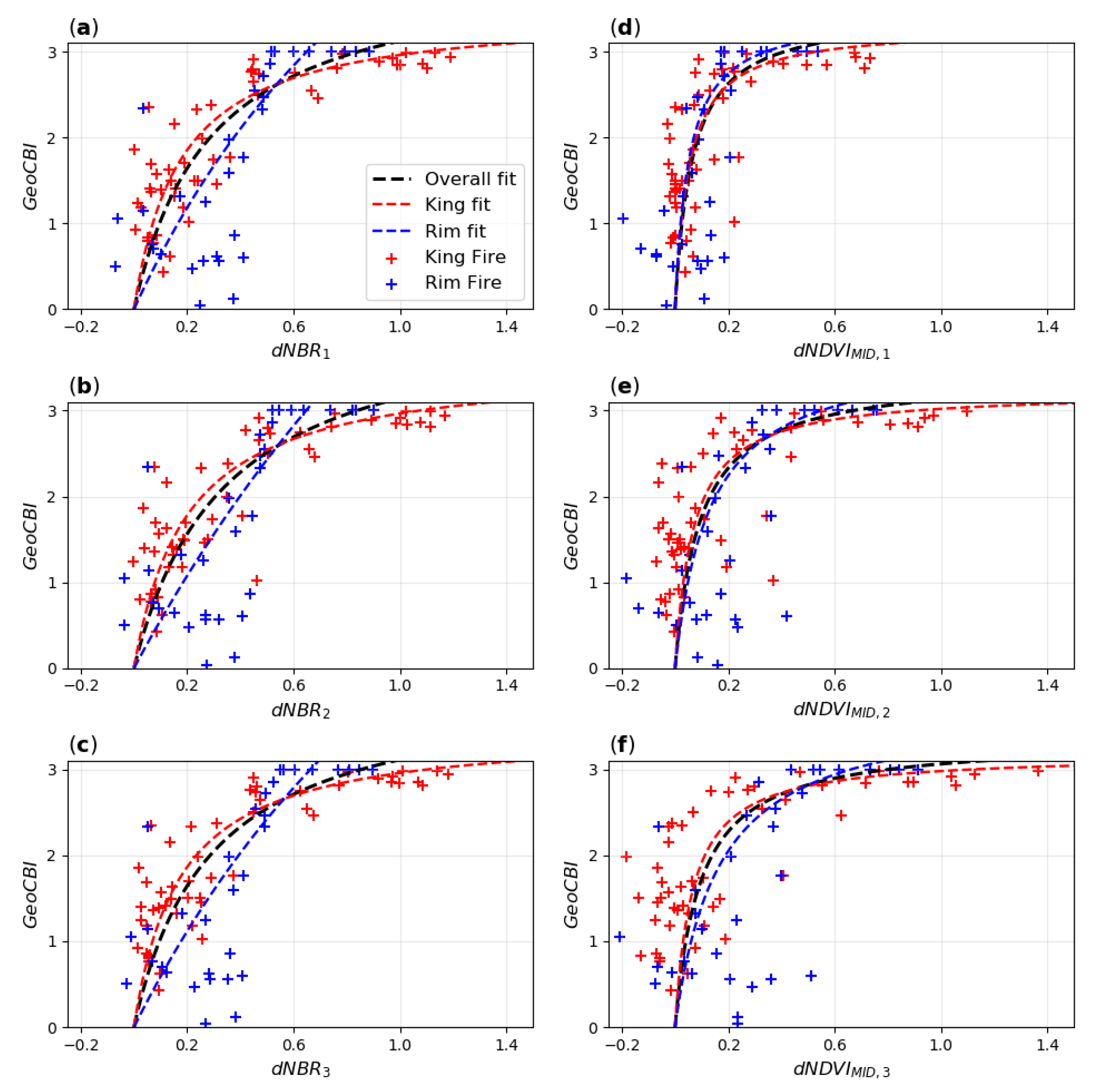
Table 4. Fitting parameters, coefficient of determination (R2) and root mean square error (RMSE) of the saturated growth regression models between spectral indices as independent variables and the Geometrically structured Composite Burn Index (GeoCBI) as dependent variable.
Rim FireKing FireOverall
abR2RMSEabR2RMSEabR2RMSE
dNBR1(a)−0.716.750.520.33−5.7019.830.810.65−3.4213.820.670.45
dNBR2(b)−0.395.800.500.32−5.0017.810.800.60−2.9512.430.660.44
dNBR3(c)−0.566.210.520.33−5.8020.160.820.66−3.4713.940.680.45
dNDVIMID,1(d)−19.5867.530.600.25−19.1663.110.576.60−15.7054.400.550.29
dNDVIMID,2(e)−7.6228.330.600.33−14.5847.070.676.65−10.7136.600.610.48
dNDVIMID,3(f)−6.0222.600.550.39−15.1548.170.687.54−10.5735.480.610.71
Note: Rows a–f contain parameter information which corresponds to the figure labels in Figure 5a–f.
Publisher’s Note: MDPI stays neutral with regard to jurisdictional claims in published maps and institutional affiliations.

