
3D Thermal Monitoring of Jointed Rock Masses through Infrared Thermography and Photogrammetry


1
Earth Sciences Department of “Sapienza” University of Rome and CERI—Research Centre for Geological Risks, P.le Aldo Moro 5, 00185 Rome, Italy
2
Acuto Field Laboratory, 03010 Acuto, Italy
*
Author to whom correspondence should be addressed.
Remote Sens. 2021, 13(5), 957; https://0-doi-org.brum.beds.ac.uk/10.3390/rs13050957
Submission received: 4 February 2021
/
Revised: 25 February 2021
/
Accepted: 27 February 2021
/
Published: 4 March 2021
(This article belongs to the Special Issue Remote Sensing for Rock Slope and Rockfall Analysis)
Abstract
:The study of strain effects in thermally-forced rock masses has gathered growing interest from engineering geology researchers in the last decade. In this framework, digital photogrammetry and infrared thermography have become two of the most exploited remote surveying techniques in engineering geology applications because they can provide useful information concerning geomechanical and thermal conditions of these complex natural systems where the mechanical role of joints cannot be neglected. In this paper, a methodology is proposed for generating point clouds of rock masses prone to failure, combining the high geometric accuracy of RGB optical images and the thermal information derived by infrared thermography surveys. Multiple 3D thermal point clouds and a high-resolution RGB point cloud were separately generated and co-registered by acquiring thermograms at different times of the day and in different seasons using commercial software for Structure from Motion and point cloud analysis. Temperature attributes of thermal point clouds were merged with the reference high-resolution optical point cloud to obtain a composite 3D model storing accurate geometric information and multitemporal surface temperature distributions. The quality of merged point clouds was evaluated by comparing temperature distributions derived by 2D thermograms and 3D thermal models, with a view to estimating their accuracy in describing surface thermal fields. Moreover, a preliminary attempt was made to test the feasibility of this approach in investigating the thermal behavior of complex natural systems such as jointed rock masses by analyzing the spatial distribution and temporal evolution of surface temperature ranges under different climatic conditions. The obtained results show that despite the low resolution of the IR sensor, the geometric accuracy and the correspondence between 2D and 3D temperature measurements are high enough to consider 3D thermal point clouds suitable to describe surface temperature distributions and adequate for monitoring purposes of jointed rock mass.
1. Introduction
The analysis of the mechanical effects in terms of induced strains by cyclical thermal stresses on rock masses is considered as a nontrivial issue in the field of geological risk mitigation relative to slope instabilities that can lead to high hazard scenarios due to their impulsiveness and high frequency of occurrence. Thus, the study of thermomechanical effects has seen an increasing interest in the last few decades. Near-surface temperature fluctuations are considered one of the least intuitive but most effective factors responsible for the progressive mechanical and physical weathering of exposed rock masses [1]. The effectiveness of near-surface thermal forcing is related to its cyclic and continuous action that can exert slight perturbations on stress fields, resulting in a day-to-day cumulative effect which eventually contributes to leading rock masses toward conditions of instability over wide time scales [2]. The superposition of heating–cooling cycles is negligible if considered in the short- to middle-term, whereas in the long-term it can influence the mechanical behavior of rock masses and act as a thermal fatigue process [2,3]. Thermal expansion–contraction cycles cause the stress fields to undergo perturbations that can induce both the growth of pre-existing cracks and the genesis of new ones in a subcritical regime (i.e., subcritical crack-growth), which is commonly associated with constant or cyclic loading [1]. These preparatory processes can induce cumulative inelastic deformations causing rock mass damage, driving it toward shallow slope failure (e.g., rockfalls and rock-topples) when transient stressors (triggers) occur [4,5]. Due to the severity and continuity of such external stressors, the analysis of thermomechanical effects on jointed rock masses requires the complete and exhaustive characterization of near-surface thermal fields. With this approach, the intensity and the evolution in time and space of temperatures can be constrained with respect to local climatic conditions, morphological features (i.e., surface irregularities and differently exposed surfaces) and jointing conditions of the target under investigation. Within this framework, infrared thermography (IRT) is considered one of the most useful tools for the characterization and monitoring of near-surface temperatures.
The fast technological development and the economic sustainability of high-resolution portable thermal cameras witnessed over the last decade have led to the increasingly widespread application of this remote surveying technique. Due to its great potential, IRT proved to be a useful non-invasive remote sensing technique in various scientific fields, from structural damage detection and energy efficiency analysis in civil engineering [6,7] to cultural heritage management and conservation [8,9]. Most IRT applications in earth sciences are related to volcanic systems monitoring, from the study of magma effusion rates [10] to the analysis of thermal anomalies related to hydrothermal systems [11]. In the last few years, novel applications of this remote surveying technique were reported in the field of engineering geology. Innovative monitoring methods were proposed to investigate temperature-related effects on jointed rock masses. Among all methods, IRT has undoubtedly demonstrated the greatest potential in studying rock mass characteristics and related hazards [12,13] as well as in defining the effect of continuous fluctuations of surface temperatures on jointed rock masses [14,15,16]. Several authors employed IRT in multitemporal monitoring surveys, highlighting the crucial role of discontinuity sets when connecting the spatial distribution and evolution of temperatures within rock masses. When open joints fall within the thermal active layer of rock masses [2], air-filled discontinuity networks can strongly influence the in-depth heat propagation, leading to fragmentation of the heat front and to the related configuration of sharp temperature contrasts across these geostructural elements [17]. Such an effect, which is induced by the contrast of thermophysical parameters between the rock matrix and the air infilling within open joints, is responsible for significant differential heating–cooling cycles of isolated sub-volumes or rock blocks. As a consequence, it is also responsible for differential thermally-induced perturbations of the local stress field. Thermal anomalies in jointed rock masses are not only induced by the existence of air-filled discontinuity networks, but they are also related to differently oriented surfaces [14,15,16]. Due to the high variability of local morphological and geostructural conditions of rock mass outcrops, the presence of exposed surfaces characterized by different orientations (dip angles and directions) can induce the appearance of nonhomogeneous distributions of surface temperatures. As a direct consequence of the differential incidence of solar radiation on the exposed surfaces, the heterogeneity of near-surface temperatures can ultimately cause the occurrence of shallow instabilities by influencing both the magnitude of rock mass thermal ranges and the evolution in space and time of surface thermal fields. The quantification of space–time variation of rock surface temperatures is also crucial for constraining the magnitude of thermal perturbations for high-resolution stress–strain thermomechanical numerical modeling [17]. The analysis of the thermomechanical behavior of jointed rock masses thus requires the characterization of the local geostructural setting (i.e., joint density and attitude) and the definition of both the amplitude and the space–time evolution of near-surface temperatures considering complex 3D geometries. Following this approach, it could be possible to retrieve nontrivial information concerning the relationship between the thermal behavior and the complex 3D geometry of the investigated area of interest.
In this study, the preliminary outcomes resulting from the integration of multitemporal IRT surveys with close-range Digital Photogrammetry (DP) are presented to characterize the thermal behavior of a jointed rock block. This research proposes a new method to describe the evolution and distribution of surface temperatures, representing them within a 3D geometrically accurate environment. The reconstruction of 3D models could significantly enhance the spectrum of analyses and interpretations concerning the relationship between jointed rock masses characteristics and their surface thermal fields. Recent developments in commercial Structure from Motion (SfM) software paved the way for the possibility to create dense point clouds starting directly from unordered and uncalibrated thermal infrared (TIR) and RGB optical images [18]. While RGB image-based terrestrial and aerial DP represents a well-established methodology for the engineering geological characterization of jointed rock masses [19,20,21], the creation of 3D TIR models represents an almost unexplored frontier. Several studies that mainly focused on the analysis of energy performances of historical buildings and industrial plants [8,22,23] proposed different approaches to fuse thermal attributes derived from IR cameras with geometrical and geospatial data obtained through the generation of 3D point clouds from Total Laser Scanner (TLS) and terrestrial or aerial photogrammetric surveys. Methodologically, these approaches deal with the draping of low-resolution TIR textures on 3D models and the co-registration of point clouds and highlight the high potential and feasibility of IRT and SfM techniques for the generation of geometrically accurate 3D thermal models. Although 3D TIR applications in engineering are continuously increasing, methodological approaches overcoming TIR images draping onto 3D models of complex rock surfaces are still limited for engineering geology purposes.
The possibility of analyzing the thermal behavior of jointed rock masses through high-quality 3D point clouds directly generated from TIR images represents a state-of-art, pioneering step toward creating new methodological approaches to characterize the thermomechanical behavior of these natural systems. In fact, while thermogram analysis can be very complicated because it is usually performed manually by the operator and without having an overall and comprehensive view of the investigated target, 3D thermal models have the potential to resolve possible issues by merging surveyed thermal and geostructural features of complex rock masses.
To address the need for 3D thermal models that are capable of describing the distribution of surface temperatures along with the morphological and geostructural setting of jointed rock masses, preliminary results from multitemporal IRT surveys of an unstable rock block are herein presented.
2. Materials and Methods
2.1. The Acuto Field Laboratory
The Acuto experimental field laboratory is located inside an abandoned quarry in the western sector of the Mt. Simbruini–Ernici ridge (Figure 1a,b), where a sedimentary succession of intensely fractured Mesozoic limestone outcrops as the result of both the compressive and extensive tectonic stages involved in the formation and evolution of the Central Apennines. The abandoned quarry was selected in late 2015 because it represented a suitable context for the implementation of a field laboratory devoted to studying the effects induced by anthropogenic and natural stressors on heavily jointed rock masses. Geomechanical surveys allowed the definition of engineering geological models for different quarry wall sectors, and a 20 m3 protruded rock block was identified as the optimal target for the installation of a multisensor and multiparametric monitoring system [24].
This potentially unstable rock block is detached from the rock wall by a subvertical and highly persistent open joint (Figure 2). The quarry wall is characterized by heights in the range between 20 and 50 m and has a N20°E direction. Because of its eastward exposure, the quarry wall is always subjected to intense direct solar radiation. Direct and indirect geomechanical surveys were performed to obtain the engineering geological model of the area dedicated to the experimental test site, and four pervasive and systematic joint sets were identified [14,25]: J0 (93/4; dip direction/dip); J1 (4/80); J2 (198/86); J3 (91/64) (Figure 2b).
Due to its geometry, the rock block is characterized by different solar exposures (Figure 1c). Two prominent orthogonal rock faces are present and are characterized by an eastward and southward exposure (respectively named as front and back faces with respect to the rock cliff direction). Such exposures combined with varied seasonal solar paths result in deferred insolation and delayed temperature maxima [14].
The monitoring system of the Acuto field laboratory was firstly instrumented with geotechnical devices to investigate the cause-effect relationship between anthropogenic and natural stressors and jointed rock masses. This includes:
- Two weather stations, at the top and the bottom of the quarry, equipped with air thermometer, hygrometer, rain gauge, and anemometer;
- One Type-K thermocouple for rock mass temperature monitoring, installed at a depth of 8 cm from the rock block surface (RT—Figure 2d);
- Six strain gauges and four extensometers installed in correspondence of microfractures and open joints, respectively.
The monitoring system was specifically designed for several experimental activities coordinated by the Research Centre for Geological Risks (CERI) of Sapienza University of Rome in the framework of the Department of Excellence Project (2018) of the Italian Ministry of Education, University and Research (MIUR). The instrumented rock block has already been targeted for several experimental remote sensing applications, including Laser Scanning, GB-InSAR, IRT and Digital Photogrammetry.
2.2. Workflow
Rock masses undergo thermal cycles due to the complex link between heating–cooling magnitudes as well as surface heterogeneity and exposure. To better evaluate the role of these effects, the 3D quantification of the distributed temperatures is required.
The present research proposes an approach for generating TIR and RGB point clouds from close-range terrestrial photogrammetric surveys to provide new insights for the characterization of jointed rock masses, as well as for future numerical modeling advances. The proposed workflow is based on the acquisition of several thermograms from different points of view around the target, following the basic principles of photogrammetric imagery acquisition to cover the investigated sector of the quarry wall completely. IRT surveys were performed in four different seasons (autumn, winter, spring and summer), collecting images at different times of the day. The reason for performing daily and seasonal monitoring surveys is related to the need to assess how morphological and geostructural conditions can constrain the rock mass thermal behavior when highly variable thermal boundary conditions exist. The acquired thermograms were processed using the Structure from Motion (SfM) software Agisoft Metashape Pro [26] for point clouds generation. The generated point clouds were then analyzed through the open-source software CloudCompare [27]. Moreover, a high-resolution DSLR camera was used to generate a reference RGB point cloud for estimating the geometric quality of TIR point clouds. Differential surface temperatures were computed and analyzed in order to investigate their distribution with respect to the main jointing and morphological features of the rock mass.
As a perspective, this study allows for the evaluation of how the generation and analysis of TIR point clouds could enhance the characterization of the thermal behavior of jointed rock masses.
2.3. Infrared Thermography Survey
Thermal imaging or Infrared Thermography (IRT) is a widely used noncontact and nondestructive remote sensing technique that provides the detailed mapping of surface temperature distributions of any object. Infrared (IR) cameras are devices generally operating in the mid-infrared band of the electromagnetic radiation spectrum (7.5–14 μm). IR sensors can quantify and convert the emitted infrared radiation into temperature values through their built-in processors [28]. The output of IR cameras is a radiometric image (i.e., thermogram) that consists of a pixel matrix describing the surface temperatures of the object under investigation. Radiometric imagery is commonly visualized through colorimetric scales that enable the recognition of thermal anomalies within or at the surface of the target through color contrasts between adjacent pixels.
Because modern IR camera functioning is very similar to digital cameras, thermogram acquisition is accomplished in a fully automatic way. Nevertheless, it is always mandatory to set the sensitivity parameters of the IR sensor which include target emissivity, distance from the target, relative position of camera and target, reflected surface temperature, air temperature and relative humidity, in order to account for a general atmospheric correction. This thermographic calibration protocol is crucial because the incoming thermal radiation (measured by the IR sensor) can be influenced by several factors that are not directly related to the object temperature. In fact, the surrounding environment and the thermal radiation angle of incidence can exert a non-negligible influence on radiometric measurements. This is due to the presence of parasite radiation and the phenomena of atmospheric partial absorption and dispersion of the emitted radiation [16,29,30].
IRT surveys were performed in autumn, winter, spring and summer, acquiring thermal images at four different hours of the day (11:30, 13:00, 16:00 and 17:00; local time) to monitor the heating and cooling stages of the jointed rock block. Thermal mapping activities were carried out during days characterized by comparable insolation and cloud coverage to reduce variability in thermal boundary conditions. This approach aimed at highlighting the thermal behavior of the rock block in different climatic conditions at the daily and seasonal time scale. The image acquisition was performed using a handheld Infrared camera (TESTO 885-1) characterized by a focal plane array (FPA) microbolometer sensor with 320 × 240 geometric resolution, operating temperature range −30 °C to 100 °C, temperature accuracy calibrated between ± 2 °C or ± 2% of measured values, spectral range of 7.5–14 μm, field of view (FOV) 30° × 24°, focal length of 15 mm and 30 mK noise equivalent temperature difference (NETD) at 30 °C. A DSLR digital camera (Canon PowerShot SX730 HS) was used during every survey to acquire optical imagery to reconstruct one high-resolution 3D point cloud representing the reference base for TIR point clouds. A monopod was employed to ensure the stability of cameras and resolve common issues in image acquisition, such as frame blurriness due to inevitable tremors of the operator. The DSLR camera calibration was achieved using the lens calibration tool of Agisoft Metashape Pro. This tool allows calibrating internal camera parameters (i.e., focal length, principal point coordinates, radial and tangential distortion coefficients) for the correct reconstruction of 3D point clouds by acquiring several images of an on-screen visualized chessboard from different observation angles. Thermal mapping of the rock block was performed following a standardized acquisition. Several control points were permanently marked on the ground before the first monitoring campaign to address the need for a complete 3D reconstruction of the rock block and to guarantee the replicability of surveys. After a preliminary calibration step of their positions, these control points were organized into a specific pattern of rays coming from the rock block (Figure 3a,b) in order to frame the target from different observation angles and distances (always within 2 and 15 m), securing a good image overlap. The adopted acquisition distances allowed the obtainment of a maximum geometric resolution of IR images in the range 3.4–25.5 mm for the closest and furthest acquisition spots, respectively.
Optical and IR images were captured from terrestrial acquisitions. Because we did not have georeferenced data or external orientation parameters at our disposal, several Ground Control Points (GCP) were placed on the investigated sector of the rock wall. The importance of model georeferencing from a relative to a global coordinate system is related to removing scale and orientation ambiguities between separately generated 3D models [18]. While natural or artificial GCPs are usually employed for optical images (e.g., geometrical markers with known dimensions and positions), it is not always feasible to find sharp and stable GCPs based only on their shape or color contrasts with the environment for IRT applications [11]. To solve the issue of GCPs for IRT surveys, seven low emissivity aluminum squared reflectors (20 × 20 cm) were employed to cover an area of 60 m2. This is because temperature differences are represented by marked contrasts in the color scale of thermograms. Aluminum foil has a mean emissivity value of 0.03–0.06 and thus reflects 94–97% of the incoming thermal radiation, thus creating high-visibility cold thermal signatures on thermograms (Figure 3c). In addition, multiple strain gauges, placed on the rock block surfaces and covered with aluminum tape for thermal insulation, were used as low emissivity GCPs for georeferencing purposes. All GCPs coordinates were extracted from a georeferenced 3D point cloud that was generated through a total station survey performed using a Leica MS60 MultiStation. The IR Camera calibration was performed before every survey and during the post-processing through the collection of specific parameters:
- Air temperature and relative humidity from the weather station located inside the field laboratory;
- The reflected temperature from the rock block surface, according to the ISO standard (ISO 18434-1);
- The distance and relative position of every acquisition spot from the target.
The value for rock mass emissivity was set to 0.94, as previously derived by Fiorucci et al. 2018 [14].
2.4. 3D TIR Point Clouds Generation
Structure from Motion (SfM) is a digital photogrammetry technique that represents one of the most affordable methods for collecting high-quality 2D and 3D geometric information of investigated areas (e.g., slopes, outcrops, structures) starting from the acquisition of a series of overlapping images [20].
The first step of the TIR point cloud generation workflow consisted of reconstructing the high-resolution optical point cloud from RGB images acquired with the DSLR camera. All images were processed using Agisoft Metashape Pro, and the resulting point cloud was georeferenced using 9 GCPs placed on the rock wall. After the optical dense point cloud was generated (9 million points dense point cloud), it was imported in CloudCompare to optimize the alignment with the reference derived by the laser scanner and from which GCPs coordinates were extracted. The alignment optimization was achieved using the Iterative Closest Point (ICP) method [31]. The ICP algorithm computes the correspondences between point clouds starting from an initial estimate for the relative rigid-body transform and iteratively refines it until the convergence is reached [18]. The ICP algorithm returned RMSE registration values in the range 0.001–0.005 m.
To process the TIR imagery, thermograms were exported as temperature matrices through the proprietary open-source software of the IR camera (TESTO-IRsoft). These matrices were converted into a floating 32bit Tiff file format through a MATLAB compiled script in order to import them into the Agisoft Metashape working environment. Because the employed IR camera does not provide EXIF data of collected thermograms, the image processing was performed relying on the automatic calibration of initial camera parameters. The first step of the SfM processing consisted of the Block Bundle Adjustment: the TIR dataset was processed by the SfM software to estimate image key-points, camera locations, orientations, and internal calibration parameters to build sparse point clouds [20]. Sparse point clouds were then manually georeferenced by identifying the low-emissivity GCPs placed on both the rock block and the adjacent quarry wall within the dataset (Figure 3c). The last step consisted of the detailed reconstruction of the investigated area by generating the dense point cloud for each IRT acquisition. The main result of this processing step is a considerable increase in point density, as described in Table 1 for one of the performed surveys.
To solve possible errors of nonperfect alignment between TIR point clouds and the high-resolution optical one, considering that because of the high density of GPCs employed for the target-based co-registration they are very close to each other in space, the alignment of TIR point clouds to the reference RGB point cloud was optimized using the ICP algorithm. Moreover, to evaluate if TIR dense point clouds were correctly generated and co-registered to the reference one and to estimate their spatial and geometric accuracy, the analysis of residual distances was performed using the Multiscale Model to Model Cloud Comparison (M3C2) algorithm implemented in CloudCompare [32]. In particular, this tool was selected over the common Cloud-to-Cloud (C2C) distance method because of its robustness in computing local residual distances and considering changes in point density and noise. Statistical parameters of residual distances between TIR and optical point clouds were computed for every survey and acquisition.
After the alignment optimization and subsequent verification steps, TIR point clouds were further processed to convert thermal attributes stored by every point from relative RGB intensity to real temperature values. In fact, even though Agisoft Metashape does not directly deal with most TIR imagery file formats, it is possible to visualize thermograms, (imported as one-band floating 32bit Tiff files) by setting a color scale according to the range of temperature values stored in the pixels matrix and applying a raster transformation to every image. Using this approach, the generated point cloud is characterized by a color-coded scalar field, and its intensity (expressed in RGB values) is directly proportional to absolute temperature values. A MATLAB script was designed to retrieve real temperature values from RGB intensities following Equation (1):
where, for the i-th point, T is the real temperature value, imin and imax represent the minimum and maximum RGB intensity values, and tmin and tmax are the minimum and maximum temperature values that were equally set for the whole TIR dataset prior to the SfM processing.
The last step of this workflow consisted of transferring the real temperature information of TIR point clouds to the reference high-resolution RGB optical point cloud. This task was accomplished using a CloudCompare built-in algorithm to perform a euclidean distance-based Nearest Neighbor Search (NNS) within TIR point clouds for every point of the reference point cloud [33]. This operation allowed the merging of temperature scalar fields of TIR point clouds to the high-density optical point cloud. To quantify the accuracy of the final output in the description of surface temperatures, a comparison between temperature distributions of original and interpolated point clouds was performed, aiming at estimating their grade of correspondence. Following this workflow, which is summarized in Figure 4, it was possible to obtain a high-resolution dense point cloud that stores temperature attributes for every seasonal survey acquisition. A comparison between 2D thermograms and 3D point clouds was performed to analyze the representativeness and reliability of TIR point clouds for the characterization of surface temperatures of the investigated rock block. In particular, two sections of interest were selected on the rock block for the extraction of temperature distribution and evolution. By availing of multitemporal (infraseasonal and infradaily) TIR point clouds, it was then possible to compute differential surface temperatures and temperature ranges at different time scales and analyze their spatial distribution with respect to the differently exposed surfaces of the rock block.
3. Results
The acquisition of more than 2400 thermograms during four intraday seasonal surveys allowed the reconstruction of 16 TIR point clouds to describe the distribution and evolution of surface temperatures of the rock block due to daily and seasonal temperature fluctuations. An example of the outcomes obtained following the proposed approach is shown in Figure 5. The visualization of 3D TIR models enhances the recognition of perceptible differences in temperature distribution patterns at different times of the day. Through the observation of the rock block from different angles, it is possible to monitor the evolution of temperatures for the whole monitoring period, evidencing how the presence of differently oriented surfaces leads to a marked heterogeneity of the surface thermal fields (Figure 5), especially during the maximum insolation stages (i.e., 11:30). This effect attenuates toward the cooling stage of the rock mass because the influence of the direct solar radiation is diminished on the irregular surface of the rock mass, and the convective heat exchange with the atmospheric air dominates the thermal balance with the outer environment. From a qualitative perspective, the 3D representation of surface temperatures allows the achievement a more comprehensive visualization of the target characteristics and enables the investigation of geospatial relationships between temperature distributions and morphological features of the rock block (i.e., differently oriented surfaces and surficial irregularities), which would be either too difficult or impossible through the observation of 2D thermograms.
After the co-registration optimization of TIR point clouds to the reference, TIR point clouds were analyzed in terms of geometric and spatial accuracy through the computation of residual distance distributions for each acquisition. This analysis was crucial because a high level of correspondence between all generated point clouds is needed to proceed with the quantitative analysis of temperature distribution and evolution. As shown in Figure 6, the results of this analysis show a high level of confidence for the co-registration optimization outcomes. Residual distances are plotted for every point cloud in a color-scaled view, enhancing the high grade of correspondence between TIR point clouds and the reference point cloud. It is worth noting that the statistical descriptors of residual distance distributions tend to vary from the first to the last acquisition performed during the survey, with median values and interdecile ranges (IDR) drifting from 0.00–0.002 m and 0.032–0.069 m, respectively. This effect was interpreted as the consequence of the net decrease in temperature contrasts within thermograms of the 16:00 and 17:00 acquisitions (Figure 6c,d) due to the progressive homogenization of surface temperatures during the cooling stage of the rock mass, which eventually affected the number of geometric details.
Moreover, the homogeneity of surface temperatures during late afternoon acquisitions is considered responsible for generating non-correspondence areas between TIR and reference point clouds. It is possible to note that in the upper-right corner of 16:00 and 17:00 point clouds, a small red area describes residual distances from the reference point cloud in the range 0.05–0.1 m. Nevertheless, considering that the uncertainties related to a nonperfect reconstruction of the rock block geometry from TIR images are clustered in small areas of the point clouds and taking into account the impossibility of acquiring more detailed thermograms during the cooling stage of the rock mass, the results of the co-registration optimization guarantee a high level of geometric detail and geospatial confidence.
After having verified the geometric accuracy of TIR point clouds and converted the thermal attributes from RGB intensity values to real temperature values (see Equation (1)), the last step of processing consisted of merging temperature scalar fields of TIR point clouds with the optical reference one. This operation aimed at creating a 3D model able to merge the high-resolution reconstruction of the rock block morphological features with surface temperature distributions recorded in different seasons and at different hours of the day.
A comparison between temperature distributions of original and merged point clouds was performed to evaluate possible errors related to the merging operation (Figure 7). From the observation of the distribution of point cloud temperature classes, it is possible to discern a high level of similarity between relative frequency distributions of different acquisitions (Figure 7a). Statistical parameters such as the mean and standard deviation of every distribution were computed to obtain a more accurate estimate of the grade of correspondence between original and merged point clouds. From the plot of Figure 7b, where the mean and standard deviation values of original and merged point clouds are shown for different acquisition times, it can be observed that only negligible shifts between these values exist. However, these temperature differences can be considered negligible because, as better highlighted in Figure 7c, mean and standard deviation values range from −0.05 °C to −0.2 °C and from 0 °C to −0.05 °C, respectively.
The obtained results demonstrate that the proposed approach produces high-confidence and geometrically accurate 3D TIR point clouds that provide information concerning both morphological features and surface temperatures of the investigated rock block.
A quantitative comparison between temperatures extracted from TIR images and 3D merged point clouds was performed to evaluate the affordability of surface thermal fields described by TIR point clouds. This analysis aimed at highlighting any significant difference in the representation of 3D surface temperatures that could be potentially related to errors inherited from the processing workflow by comparing TIR point clouds with the well-established technique of temperature extraction from 2D thermograms.
Two cross-sections (AB–CD) which belong to different rock block sectors and are characterized by different exposures and degree of surficial roughness were selected for the extraction of temperature distributions relative to one of the performed seasonal surveys (Figure 8a–d). Section AB is located on the southeastward surface of the rock block and is characterized by a smooth and regular surface. On this section, temperature distributions tend to show spatial homogeneity, which highlighted no significant thermal contrasts for the entire profile length (Figure 8f). The homogeneity of temperature distributions is evident for values extracted from both thermograms and TIR point clouds. Only slight differences arise between 2D and 3D temperature distributions (Figure 8h), but because they are within the confidence interval of the IR camera measurement sensitivity (±2 °C buffer zone), they can be considered negligible. Section CD is located on the southward surface of the rock block and is characterized by a scattered and irregular profile. This section exhibits a more complex and heterogeneous spatial distribution of temperatures (Figure 8g). In particular, temperature heterogeneities are evident during the heating phase of the rock mass (between 11:30 and 13:00—red and yellow lines respectively), when spatial thermal contrasts exceed 5 °C. Moreover, sharp thermal contrasts emerge for the entire length of the analyzed section, highlighting the existence of high spatial gradients of temperature. This effect attenuates at the end of the heating phase when the rock mass enters its cooling phase (16:00–17:00, green and blue lines, respectively). Similarly, differences in temperature distributions recorded by 2D thermograms and 3D point clouds are always within the ±2 °C confidence interval and have their maximum values at the 13:00 acquisition (Figure 8i) and progressively decrease toward homogeneity between 2D and 3D extracted values during the cooling phase. The heterogeneity of temperature distributions analyzed along section CD can be interpreted as a consequence of the irregularities and asperities characterizing the rock mass surface. Even the limited protruded elements are capable of shadowing adjacent areas, which is not only responsible for generating areas that are not directly exposed to the incident solar radiation but also for originating non-negligible spatial temperature gradients. It is also worth noting that the relative position of camera and target could play a role in the generation of nonhomogeneous temperature distributions, especially if a significant roughness and irregularity characterize exposed surfaces. Furthermore, when the solar radiation is diminished and the thermal convection dominates the heat balance (during cooling stages of the rock mass) [14,15], the attenuation of spatial temperature gradients strengthens the hypothesis of a significant interaction between differently exposed surfaces and the incident solar radiation [34].
As a result of the geometric and thermal validation of merged TIR point clouds (Figure 6 and Figure 7), as well as due to the high grade of correspondence between temperature values extracted from 3D models and 2D thermograms (Figure 8), each point of the point clouds (Pi) affordably stores 3D coordinates and multitemporal temperatures, Pi (Xi, Yi, Zi, T1i, …, Tni). Starting from the high-resolution TIR point cloud storing multiple thermal parameters, it was possible to compute the distribution of daily surface temperature ranges for the investigated rock block. Following the above-described method, a point cloud containing temperature information collected during every acquisition of each seasonal survey was created. This step allowed the creation of three merged TIR point clouds characterized by four different thermal attributes (e.g., 11:30, 13:00, 16:00 and 17:00) and the maximum and minimum temperature values recorded during all acquisitions were retrieved for every point of TIR point clouds by implementing a MATLAB routine. The computation of the difference between these values enabled the reconstruction of the distribution of temperature ranges for the rock block (Figure 9).
As shown in Figure 9, where the outcomes of this analysis are presented in the form of point clouds and frequency distribution histograms, daily temperature ranges appear to significantly vary in terms of absolute amplitude and spatial distribution during the four seasonal surveys, even though cloud coverage and insolation conditions were considered comparable. This color-scale visualization allows appreciating the distribution of temperature ranges on the rock block surface, highlighting areas that were subjected to different thermal stress amplitudes. The greatest temperature ranges were recorded during the winter and spring monitoring surveys when the median value (P50) reached respectively 7.1 °C and 6.9 °C, whereas in summer and autumn it reached 3.3 °C and 4.1 °C (Figure 9).
Moreover, temperature values associated with the 25th and 75th percentiles (P25 and P75) are highlighted in all histograms to mark significant deviations in temperature range distributions. To further analyze the variability of the rock block thermal behavior in response to different meteo-climatic conditions, the percentile corresponding to a temperature range greater than 8 °C was computed.
This statistical descriptor helps to quantify the point cloud percentage that showed considerable thermal stress in the four seasonal campaigns. It can be observed from the histograms of Figure 9 that in autumn and summer surveys only 11–12% of the point cloud exhibited temperature ranges greater than 8 °C. Differently, in the spring and winter surveys 38% and 42% of the point cloud underwent significant temperature fluctuations. Such a result enables the observation of the amplitude and spatial distribution of surface temperature ranges as well as the quantification of nontrivial information concerning the thermal behavior of the rock block under variable climatic conditions within a 3D geometrically accurate environment.
This approach can be devoted to the reconstruction of 3D models that can concurrently store multitemporal temperature values and 3D coordinates (X, Y, Z). The obtained model provides a tool to deepen the relationship between 3D features and thermal processes by evaluating the effect of shadowing and geometric irregularities on the resulting temperature distribution.
In this framework, a preliminary attempt was made to analyze the correlation between differently exposed surfaces of the rock block and recorded temperature ranges, relying on the consideration of point cloud dip and dip direction values. These two parameters were selected to describe the spatial orientation variability of the rock block surfaces and were derived from the computation of point cloud normal vectors in Cloud Compare via estimation of local surface models interpolating point neighbors. Because the distribution of point cloud dip angles showed a significant tendency toward very high values (Figure 10a), highlighting how 73% (P27) and 50% (P50) of the point cloud are characterized by dip angles higher than 60° and 75° (Figure 10b), this parameter was neglected during the analysis by assuming a constant subvertical inclination.
This approximation is admissible because of the overall subvertical configuration of the rock block that is derived from both the steepness of the rock wall and the existence of high angle joint sets affecting its integrity. In light of these considerations, all point clouds were classified only by taking into account the dip direction parameter.
Eight classes were defined to represent the main differences in the orientation of the rock block surfaces considering dip direction values variability. Points belonging to surfaces with equal orientation were clustered. The color-coded 3D representation of the eight dip direction classes, shown in panels a and b of Figure 11, highlights a considerable differentiation of exposure classes of the rock block surfaces. Even though all classes were singularly treated and analyzed, it was decided that opposite classes should be represented by assigning congruent colors. Due to the direction of the rock wall and the overall subverticality of the rock block surfaces, opposite dip direction classes are characterized by the same exposure. The only non-negligible differences that may arise between high-angle surfaces characterized by opposite dip directions could be related to local morphological conditions, such as overhanging rock volumes or large-scale surficial irregularities. However, a preliminary manual identification should be performed in order to take into account local surficial features. All points belonging to each directional class were extracted, and the distribution of temperature ranges was computed for every cluster. A normal distribution was then applied to retrieve the mean and standard deviation values of every distribution. This step quantitatively merges thermal and geospatial information of 3D point clouds by relating specific temperature attributes to each dip direction class.
The results of this analysis are presented as polar plots (Figure 11c) and describe the relationship between the seasonal thermal forcing and the rock block surfaces characterized by different orientations. The polar plots enable the ability to infer how the amplitude of temperature ranges varies depending on the orientation of surfaces exposed to the incident solar radiation. Even though significant differences in absolute temperature ranges arise between different seasonal records, the enhanced visualization of directional classes (i.e., E, SE and S) that experienced the relative greatest temperature ranges is provided. Despite the need for new IRT acquisitions to achieve good data redundancy, it should be noted that the independence from different seasonal thermal boundary conditions of the greatest temperature range distributions on the same directional classes represents a significant and nonrandom result, as highlighted by Figure 11. The pattern of temperature range distributions clustered on surfaces characterized by eastward to southward dip directions can be interpreted as the consequence of an almost perfect alignment to the solar path trajectories during the heating phase of the rock mass. The probability of experiencing greater daily thermal stress on surfaces therefore strongly depends on the local surface shapes, exposures, and geological conditions. Local morphological features of rock slopes can strongly constrain the insolation homogeneity (e.g., in terms of magnitude and distribution). Surface shapes and geological elements such as the N20°E direction of the rock wall and the high-angle joint sets (J1, J2 and J3, Figure 2b) could be considered as primary causes of the observed directional differentiation of temperature range distributions because they contribute to the generation of a complex geometry characterized by surfaces with heterogeneous exposures.
4. Discussion
The increasing interest in thermally-induced effects on jointed rock masses [17,35,36,37,38,39,40,41] requires an improvement in the techniques for temperature field analysis to integrate traditional direct contact methods [14,42]. In this sense, IRT surveys support the quantitative study of surface temperature fields over rock slopes, deriving distributed maps at their external interface. For rock slopes and cliffs which are characterized by a high geometric complexity given by the existence of rock columns, overhanging blocks and hollows, the 3D reconstruction of thermal fields can become paramount even at the expense of radiometric image resolution.
Several approaches have been proposed so far which adopt the exclusive draping of TIR textures onto 3D models [28]. The main disadvantage of thermal draping resides in the lack of interrogable quantitative information that could allow operations between multiple (e.g., multitemporal) thermal point clouds, characterized by 3D coordinates (X, Y, Z) and additional temperature attributes. In this framework, co-registered images composed of IR and Visible wavelengths are starting to be used in rigorous engineering approaches [23], while multistage and separate SfM processing appears to be both robust and cost-effective [11,33,43,44].
A simplified approach based on merging multitemporal 3D TIR and RGB optical point clouds derived by SfM processing is here proposed for natural rock slopes as well as geological heritage and cultural heritage monitoring applications. The obtained results shed light on the applicability of SfM methods based on the co-acquisition of TIR and RGB optical imagery in order to reconstruct 3D fused models. The main focus of the proposed workflow is represented by the possibility to gather multiple advantages from the fusion of multitemporal TIR and RGB optical point clouds. In fact, while the co-registration via target-based techniques (GCPs registration) and fine registration methods (ICP) allows achieving an optimized alignment of TIR and optical point clouds, the fusion of real temperature values with high-resolution point clouds results in an enhanced representation of surface temperature fields. Consequently, multitemporal thermal information can be stored by a single high-resolution 3D model, enabling the computation of temperature gradients and ranges for the monitoring target. The potential of this approach lies in the possibility of obtaining queryable models that can describe surface temperature fluctuations of targets as well as deepen existing relationships between morphological features of rock masses and their continuously varying thermal boundary conditions. While the quantification of common thermal indexes(e.g., thermal gradients) can be achieved by acquiring 2D thermograms through standard IRT surveys, the study of the relationships between these indexes and the geospatial and geological characteristics of exposed surfaces (i.e., dip direction, dip angles, surface roughness, lithology and jointing conditions) can only be approached by availing correctly scaled and oriented 3D models, which need to provide accurate geometric and thermal information.
Some limitations exist and need to be highlighted concerning the proposed methodological approach. In this case study, the investigation of a limited and easily accessible sector of the quarry wall through terrestrial acquisitions of thermograms from very close distances (2–15 m) allowed the obtainment of high ground sampling distances (GSD), in the range of 3.4–25.5 mm. This resulted in a detailed reconstruction of 3D TIR point clouds. On the contrary, when investigating more extended areas or when greater distances of acquisition are required (e.g., not accessible steep sea cliffs or mountain walls), the consequent loss in thermograms resolution could directly impact the quality of 3D models. From a general perspective, thermal resolution issues can be resolved by employing higher resolution IR sensors, even though high-quality results were achieved by acquiring thermograms from great distances [11,33]. Another nontrivial factor limiting the applicability of this approach is represented by the need to avail a good amount of GCPs, which need to be identified by both the IR and optical cameras. Target positioning is essential for the independent reconstruction and absolute georeferencing of point clouds (TIR and optical). Additionally, when there is a lack of encoded metadata containing exterior orientation parameters of cameras (as in this case study) target positioning represents the only solution for a reliable 3D reconstruction of the scanned scene. Consequently, when inaccessible or high-risk sites represent monitoring areas, especially in engineering geological issues, the task of target positioning may not be feasible [45,46]. A possible approach to partially solve this problem is the employment of UAV platforms equipped with Real Time Kinematic Global Positioning Systems (RTKGPS) [47] that can provide camera positions with high accuracy (i.e., errors in the order of centimeters). However, a persisting issue could still be the need for finding elements that are identifiable by the IR sensor. In order to reduce the uncertainties in the reconstruction of surface temperatures related to the dependence of apparent emissivity from the relative position of camera and target [48], future applications should take into account the variability of this parameter for different observation angles.
The technological advance in the characteristics of commercial IR sensors, along with the development of super-resolution algorithms, can determine a significant improvement in the geometric resolution of 3D outputs and lead to providing detailed information even on small scale elements or objects. In this sense, the use of UAV platforms with built-in or mounted IR cameras can push the boundary of performances for 3D thermal reconstructions, allowing the collection of detailed and homogeneously distributed imagery across several spectral bands. The employment of UAVs will also support the investigation of wider sectors of rock slopes and cliffs involved in instability processes, where extensive coverages and long acquisition distances are required [16,28]. While the approach adopted here guarantees a rapid acquisition for multitemporal daily monitoring purposes, UAV acquisitions could potentially enhance the accuracy of 3D models by ensuring reduced acquisition time intervals and avoiding significant changes in temperature conditions during fast heating or cooling ramps [14,15].
As a principal application, the acquisition of multitemporal daily and seasonal fused thermal and optical models will support the quantification of thermal conditions acting at the boundary of potentially unstable rock volumes (identified a priori by kinematic compatibility analyses). Field-based or remote surveys of the existing jointing conditions can be pursued, deriving the envelope of poles of discontinuities that dip in a kinematically viable way and that are dynamically compatible with planar slides or wedge movements (Figure 12a).
On the exposed facets of joint sets and nonsystematic discontinuities, daily and seasonal amplitudes of thermal stress can be quantitatively assessed (Figure 12b), specifically evaluating the effects of variable rates in heating and cooling cycles. The accurate 3D geometric reconstruction of surface temperature fields would thus provide further insights for the assessment of the role played by preparatory thermal stresses in the distribution of elastic and plastic deformation in jointed rock masses [2], weighting the contribution of lighting and shadowing effects on slopes or block volumes featured by variable exposures and hence differentially heated by the solar radiation [3,49].
With the upcoming rise in IR sensors resolution, the role of open joints in constraining the behavior of isolated rock blocks could be better understood by estimating the conditions in which joint sets can thermally influence their stability [14]. In this sense, distributed and multitemporal 3D models (both optical and thermal) can support and improve the knowledge of cause-effect relationships between thermal forcing and induced deformation when they are integrated with information of displacement/strain field that are derived by either TLS surveys and Change Detection analyses or geotechnical devices (e.g., strain gauges or extensometers).
As a future perspective, multitemporal TLS surveys will be performed at the Acuto field laboratory to detect detachment zones of rockfall or slides that are not relatable to transient pluviometric and seismic triggers, with the aim of comparing them with sectors characterized by peculiar thermal and exposure conditions (Figure 13).
On target elements, the continuous acquisition and processing of thermal images would also enrich the monitoring activities that are aimed at understanding how and when thermomechanical actions are more effective over continuously varying climatic conditions.
On selected protruded rock blocks which are considered as geostructurally predisposed to instability and mechanically prepared by the continuous action of thermal cycles over seasons (e.g., in Figure 13), the role of differential heating–cooling cycles will be evaluated while considering strain effects cumulated across joints by the day-to-day repetition of dilation and contraction phases. Furthermore, quantitative studies will be approached via numerical and laboratory analyses in order to understand the time needed by preparatory actions to cause failure in kinematically predisposed sectors. At the same time, the influence of weak triggering forces (posed by induced vibration or self-induced oscillations) in inducing instability will be dealt with by considering several evolutionary stages of constant rate processes such as internal resistance decreases due to rock weathering [50], progressive rock mass damaging, fatigue or creep processes [51,52] and the accumulation of slight and irreversible subcritical plastic deformations [53,54,55], weighting their contribution in the rockfall hazard.
5. Conclusions
Thermal processes in jointed rock masses can be responsible for deformative effects across weak joints, where genesis and progressive growth are amongst the least trivial processes in rock mechanics. Although the mechanisms driving cumulative inelastic strain on short- to long-term time scales are relatively well established, the timing and localization (i.e., when and where) of failure events is still far from being well understood and described. A priori knowledge concerning how near-surface heating and cooling processes affect complex natural systems (e.g., rock slopes or cliffs) is required to address this challenge. To this aim, a practical approach was tested. The approach was devoted to the generation of multitemporal thermal point clouds and the reconstruction of fused 3D visible and thermal models.
The adopted simplified method integrating SfM and IRT revealed that through the generation and co-registration of TIR and optical RGB point clouds, the transfer of thermal attributes from low- to high-density point clouds results in a composite output that provides a detailed and accurate 3D representation of geometric features and surface temperature distributions.
The suitability of the proposed method for the purpose of monitoring jointed rock masses lies in better understanding of the existing relationships between continuous temperature fluctuations and geomechanical and geomorphological conditions of jointed rock masses. In fact, through the conversion of temperature scalar fields from relative RGB intensities to real temperature values as well as availing of geometrically accurate 3D models that can describe even small details of rock mass surfaces, merged point clouds not only enhance the identification of sectors experiencing significant thermal stresses, but they also make it possible to quantitatively investigate correlations between rock mass jointing and local morphological conditions.
These results represent the basis for further advances in the analysis of thermally-induced effects on rock masses through numerical modeling methods. The exploitation of thermal point clouds could provide a useful tool to better understand cause–effect relationships between near-surface thermal stresses and induced deformation by constraining the spatial distribution and temporal evolution of temperature fields in the 3D space. Multitemporal 3D thermal models will also support numerical modeling analyses devoted to the reconstruction of heat transfer processes in 3D that can condition the thermomechanical response of jointed rock masses over different space and time scales.
Author Contributions
Conceptualization, G.G., M.F. and G.M.M.; Data curation, G.G.; Formal analysis, G.G.; Funding acquisition, G.G., G.M.M. and S.M.; Investigation, G.G., M.F. and G.M.M.; Methodology, G.G., M.F. and G.M.M.; Project administration, G.G., M.F., G.M.M. and S.M.; Resources, G.G., M.F. and G.M.M.; Software, G.G.; Supervision, S.M.; Validation, G.G.; Visualization, G.G. and G.M.M.; Writing–original draft, G.G. and G.M.M.; Writing–review & editing, G.G., M.F., G.M.M. and S.M. All authors have read and agreed to the published version of the manuscript.
Funding
This study has been supported by Italian Ministry of Education, Universities and Research—Dipartimenti di Eccellenza—L. 232/2016. The research is also funded by the projects “Characterization of the thermal behaviour of rock masses through Infrared Thermography and Digital Photogrammetry” (Sapienza University of Rome—Year 2020, P.I. Guglielmo Grechi), “Analysis of 2D and 3D thermal response of rocks and soils in landslide triggering conditions through site and laboratory experiments” (Sapienza University of Rome—Year 2019, P.I. Gian Marco Marmoni) and “Rock failures in cliff slopes: from back- to forward-analysis of processes through monitoring and multi-modeling approaches” (Sapienza University of Rome—Year 2016, P.I. Salvatore Martino).
Institutional Review Board Statement
Not applicable.
Informed Consent Statement
Not applicable.
Data Availability Statement
MATLAB codes presented in this study are available on request from the corresponding author.
Acknowledgments
The Authors wish to acknowledge the Municipality of Acuto for allowing the experimental activities in the quarry and the three anonymous reviewers for their constructive suggestions that improved the quality of the manuscript.
Conflicts of Interest
The authors declare no conflict of interest.
References
- Eppes, M.C.; Magi, B.; Hallet, B.; Delmelle, E.; Mackenzie-Helnwein, P.; Warren, K.; Swami, S. Deciphering the role of solar-induced thermal stresses in rock weathering. Bull. Geol. Soc. Am. 2016, 128, 1315–1338. [Google Scholar] [CrossRef] [Green Version]
- Gunzburger, Y.; Merrien-Soukatchoff, V.; Guglielmi, Y. Influence of daily surface temperature fluctuations on rock slope stability: Case study of the Rochers de Valabres slope (France). Int. J. Rock Mech. Min. Sci. 2005, 42, 331–349. [Google Scholar] [CrossRef]
- Hall, K. The role of thermal stress fatigue in the breakdown of rock in cold regions. Geomorphology 1999, 31, 47–63. [Google Scholar] [CrossRef]
- Bakun-Mazor, D.; Hatzor, Y.H.; Glaser, S.D.; Carlos Santamarina, J. Thermally vs. seismically induced block displacements in Masada rock slopes. Int. J. Rock Mech. Min. Sci. 2013, 61, 196–211. [Google Scholar] [CrossRef]
- Collins, B.D.; Stock, G.M. Rockfall triggering by cyclic thermal stressing of exfoliation fractures. Nat. Geosci. 2016, 9, 395–400. [Google Scholar] [CrossRef]
- Kylili, A.; Fokaides, P.A.; Christou, P.; Kalogirou, S.A. Infrared thermography (IRT) applications for building diagnostics: A review. Appl. Energy 2014, 134, 531–549. [Google Scholar] [CrossRef]
- Barreira, E.; Almeida, R.M.S.F.; Simões, M.L.; Rebelo, D. Quantitative Infrared thermography to evaluate the humidification of lightweight concrete. Sensors 2020, 20, 1664. [Google Scholar] [CrossRef] [Green Version]
- Cabrelles, M.; Galcerá, S.; Navarro, S.; Lerma, J.L.; Akasheh, T.; Haddad, N. Integration of 3D laser scanning, photogrammetry and thermography to record architectural monuments. In Proceedings of the 22nd International CIPA Symposium, Kyoto, Japan, 11–15 October 2009; Volume 9, pp. 3–8. [Google Scholar]
- Grinzato, E. IR thermography applied to the cultural heritage conservation. In Proceedings of the 18th World Conference on Nondestructive Testing, Durban, South Africa, 16–20 April 2012; Volume 2. [Google Scholar]
- Sansivero, F.; Vilardo, G. Processing thermal Infrared imagery time-series from volcano permanent ground-based monitoring network. Latest methodological improvements to characterize surface temperatures behavior of thermal anomaly areas. Remote Sens. 2019, 11, 553. [Google Scholar] [CrossRef] [Green Version]
- Della Seta, M.; Esposito, C.; Fiorucci, M.; Marmoni, G.M.; Martino, S.; Sottili, G.; Belviso, P.; Carandente, A.; de Vita, S.; Marotta, E.; et al. Thermal monitoring to infer possible interactions between shallow hydrothermal system and slope-scale gravitational deformation of Mt. Epomeo (Ischia Island, Italy). Geol. Soc. Spec. Publ. Volcan. Island Hazard Assess. Risk Mitig. 2021, in press. [Google Scholar]
- Teza, G. Thimran: Matlab toolbox for thermal image processing aimed at damage recognition in large bodies. J. Comput. Civ. Eng. 2014, 28, 1–8. [Google Scholar] [CrossRef]
- Mineo, S.; Pappalardo, G.; Rapisarda, F.; Cubito, A.; Di Maria, G. Integrated geostructural, seismic and Infrared thermography surveys for the study of an unstable rock slope in the Peloritani Chain (NE Sicily). Eng. Geol. 2015, 195, 225–235. [Google Scholar] [CrossRef]
- Fiorucci, M.; Marmoni, G.M.; Martino, S.; Mazzanti, P. Thermal response of jointed rock masses inferred from Infrared thermographic surveying (Acuto test-site, Italy). Sensors 2018, 18, 2221. [Google Scholar] [CrossRef] [Green Version]
- Grechi, G.; Martino, S. Preliminary results from multitemporal infrared thermography surveys at the wied-il-mielah rock arch (island of gozo). Ital. J. Eng. Geol. Environ. 2019, 1, 41–46. [Google Scholar] [CrossRef]
- Guerin, A.; Jaboyedoff, M.; Collins, B.D.; Derron, M.H.; Stock, G.M.; Matasci, B.; Boesiger, M.; Lefeuvre, C.; Podladchikov, Y.Y. Detection of rock bridges by Infrared thermal imaging and modeling. Sci. Rep. 2019, 9, 1–19. [Google Scholar] [CrossRef] [Green Version]
- Marmoni, G.M.; Fiorucci, M.; Grechi, G.; Martino, S. Modelling of thermo-mechanical effects in a rock quarry wall induced by near-surface temperature fluctuations. Int. J. Rock Mech. Min. Sci. 2020, 134, 104440. [Google Scholar] [CrossRef]
- Maset, E.; Fusiello, A.; Crosilla, F.; Toldo, R.; Zorzetto, D. PHOTOGRAMMETRIC 3D BUILDING RECONSTRUCTION from THERMAL IMAGES. ISPRS Ann. Photogramm. Remote Sens. Spat. Inf. Sci. 2017, 4, 25–32. [Google Scholar] [CrossRef] [Green Version]
- Sturzenegger, M.; Stead, D. Quantifying discontinuity orientation and persistence on high mountain rock slopes and large landslides using terrestrial remote sensing techniques. Nat. Hazards Earth Syst. Sci. 2009, 9, 267–287. [Google Scholar] [CrossRef]
- Westoby, M.J.; Brasington, J.; Glasser, N.F.; Hambrey, M.J.; Reynolds, J.M. “Structure-from-Motion” photogrammetry: A low-cost, effective tool for geoscience applications. Geomorphology 2012, 179, 300–314. [Google Scholar] [CrossRef] [Green Version]
- Francioni, M.; Simone, M.; Stead, D.; Sciarra, N.; Mataloni, G.; Calamita, F. A new fast and low-cost photogrammetry method for the engineering characterization of rock slopes. Remote Sens. 2019, 11, 1267. [Google Scholar] [CrossRef] [Green Version]
- Scaioni, M.; Rosina, E.; L’erario, A.; Dìaz-Vilariño, L. Integration of Infrared thermography & photogrammetric surveying of built landscape. Int. Arch. Photogramm. Remote Sens. Spat. Inf. Sci. ISPRS Arch. 2017, 42, 153–160. [Google Scholar] [CrossRef] [Green Version]
- Javadnejad, F.; Gillins, D.T.; Parrish, C.E.; Slocum, R.K. A photogrammetric approach to fusing natural colour and thermal Infrared UAS imagery in 3D point cloud generation. Int. J. Remote Sens. 2019, 41, 211–237. [Google Scholar] [CrossRef]
- D’Angiò, D.; Fantini, A.; Fiorucci, M.; Grechi, G.; Iannucci, R.; Marmoni, G.M.; Martino, S.; Lenti, L. Multisensor Monitoring for Detecting Rock Wall Instabilities from Precursors to Failures: The Acuto Test-Site (Central Italy); ISRM International Symposium—EUROCK: Trondheim, Norway, 2020. [Google Scholar]
- Fantini, A.; Fiorucci, M.; Martino, S.; Paciello, A. Investigating Rock Mass Failure Precursors Using a Multi-Sensor Monitoring System: Preliminary Results from a Test-Site (Acuto, Italy). Procedia Eng. 2017, 191, 188–195. [Google Scholar] [CrossRef]
- Agisoft Metashape (Version 1.5.1) 2019. Available online: https://www.agisoft.com/ (accessed on 1 March 2021).
- CloudCompare V 2.11.3, GPL Software 2020. Available online: http://www.cloudcompare.org/ (accessed on 1 March 2021).
- Frodella, W.; Elashvili, M.; Spizzichino, D.; Gigli, G.; Adikashvili, L.; Vacheishvili, N.; Kirkitadze, G.; Nadaraia, A.; Margottini, C.; Casagli, N. Combining Infrared thermography and UAV digital photogrammetry for the protection and conservation of rupestrian cultural heritage sites in Georgia: A methodological application. Remote Sens. 2020, 12, 892. [Google Scholar] [CrossRef] [Green Version]
- Prendes-Gero, M.B.; Suárez-Domínguez, F.J.; González-Nicieza, C.; Álvarez-Fernández, M.I. Infrared Thermography Methodology Applied to Detect Localized Rockfalls in Self-Supporting Underground Mines; ISRM International Symposium—EUROCK: Wroclaw, Poland, 2013; pp. 825–829. [Google Scholar] [CrossRef]
- Pappalardo, G.; Mineo, S.; Zampelli, S.P.; Cubito, A.; Calcaterra, D. Infrared Thermography proposed for the estimation of the Cooling Rate Index in the remote survey of rock masses. Int. J. Rock Mech. Min. Sci. 2016, 83, 182–196. [Google Scholar] [CrossRef]
- Rusinkiewicz, S.; Levoy, M. Efficient variants of the ICP algorithm. In Proceedings of the Third International Conference on 3-D Digital Imaging and Modeling, Quebec City, QC, Canada, 28 May–1 June 2001; pp. 145–152. [Google Scholar] [CrossRef] [Green Version]
- Lague, D.; Brodu, N.; Leroux, J. Accurate 3D comparison of complex topography with terrestrial laser scanner: Application to the Rangitikei canyon (N-Z). ISPRS J. Photogramm. Remote Sens. 2013, 82, 10–26. [Google Scholar] [CrossRef] [Green Version]
- Guilbert, V.; Antoine, R.; Heinkelé, C.; Maquaire, O.; Costa, S.; Gout, C.; Davidson, R.; Sorin, J.L.; Beaucamp, B.; Fauchard, C. Fusion of thermal and visible point clouds: Application to the Vaches Noires Landslide, Normandy, France. Int. Arch. Photogramm. Remote Sens. Spat. Inf. Sci. ISPRS Arch. 2020, 43, 227–232. [Google Scholar] [CrossRef]
- Chicco, J.M.; Vacha, D.; Mandrone, G. Thermo-physical and geo-mechanical characterization of faulted carbonate rock masses (Valdieri, Italy). Remote Sens. 2019, 11, 179. [Google Scholar] [CrossRef] [Green Version]
- Sharma, P.; Verma, A.K.; Negi, A.; Jha, M.K.; Gautam, P. Stability assessment of jointed rock slope with different crack infillings under various thermomechanical loadings. Arab. J. Geosci. 2018, 11, 1–16. [Google Scholar] [CrossRef]
- Bakun-Mazor, D.; Keissar, Y.; Feldheim, A.; Detournay, C.; Hatzor, Y.H. Thermally-Induced Wedging–Ratcheting Failure Mechanism in Rock Slopes. Rock Mech. Rock Eng. 2020, 53, 2521–2538. [Google Scholar] [CrossRef]
- Taboada, A.; Ginouvez, H.; Renouf, M.; Azemard, P. Landsliding generated by thermomechanical interactions between rock columns and wedging blocks: Study case from the Larzac Plateau (Southern France). EPJ Web Conf. 2017, 140, 14012. [Google Scholar] [CrossRef]
- Alcaíno-Olivares, R.; Perras, M.A.; Ziegler, M.; Leith, K. Thermo-mechanical cliff stability at tomb KV42 in the Valley of the Kings, Egypt. In Understanding and Reducing Landslide Disaster Risk; Sassa, K., Mikoš, M., Sassa, S., Bobrowsky, P.T., Takara, K., Dang, K., Eds.; WLF 2020. ICL Contribution to Landslide Disaster Risk Reduction; Springer: Cham, Switzland, 2021. [Google Scholar] [CrossRef]
- Grechi, G.; Martino, S. Multimethodological study of non-linear strain effects induced by thermal stresses on jointed rock masses. In Understanding and Reducing Landslide Disaster Risk; Sassa, K., Mikoš, M., Sassa, S., Bobrowsky, P.T., Takara, K., Dang, K., Eds.; WLF 2020. ICL Contribution to Landslide Disaster Risk Reduction; Springer: Cham, Switzland, 2021. [Google Scholar] [CrossRef]
- Collins, B.D.; Stock, G.M.; Eppes, M.C. Relaxation Response of Critically Stressed Macroscale Surficial Rock Sheets. Rock Mech. Rock Eng. 2019, 52, 5013–5023. [Google Scholar] [CrossRef]
- Greif, V.; Brcek, M.; Vlcko, J.; Varilova, Z.; Zvelebil, J. Thermomechanical behavior of Pravcicka Brana Rock Arch (Czech Republic). Landslides 2016, 14, 1441–1455. [Google Scholar] [CrossRef]
- Guerin, A.; Jaboyedoff, M.; Collins, B.D.; Stock, G.M.; Derron, M.H.; Abellán, A.; Matasci, B. Remote thermal detection of exfoliation sheet deformation. Landslides 2020. [Google Scholar] [CrossRef]
- Ham, Y.; Golparvar-Fard, M. An automated vision-based method for rapid 3D energy performance modeling of existing buildings using thermal and digital imagery. Adv. Eng. Informatics 2013, 27, 395–409. [Google Scholar] [CrossRef]
- Sledz, A.; Unger, J.; Heipke, C. Thermal IR imaging: Image quality and orthophoto generation. Int. Arch. Photogramm. Remote Sens. Spat. Inf. Sci. ISPRS Arch. 2018, 42, 413–420. [Google Scholar] [CrossRef] [Green Version]
- Thiele, S.T.; Varley, N.; James, M.R. Thermal photogrammetric imaging: A new technique for monitoring dome eruptions. J. Volcanol. Geotherm. Res. 2017, 337, 140–145. [Google Scholar] [CrossRef] [Green Version]
- Melis, M.T.; Da Pelo, S.; Erbì, I.; Loche, M.; Deiana, G.; Demurtas, V.; Meloni, M.A.; Dessì, F.; Funedda, A.; Scaioni, M.; et al. Thermal remote sensing from UAVs: A review on methods in coastal cliffs prone to landslides. Remote Sens. 2020, 12, 1971. [Google Scholar] [CrossRef]
- Kalacska, M.; Lucanus, O.; Arroyo-Mora, J.P.; Laliberté, É.; Elmer, K.; Leblanc, G.; Groves, A. Accuracy of 3d landscape reconstruction without ground control points using different uas platforms. Drones 2020, 4, 13. [Google Scholar] [CrossRef] [Green Version]
- Cuenca, J.; Sobrino, J.A. Experimental measurements for studying angular and spectral variation of thermal infrared emissivity. Appl. Opt. 2004, 43, 4598–4602. [Google Scholar] [CrossRef]
- Gunzburger, Y.; Merrien-Soukatchoff, V. Near-surface temperatures and heat balance of bare outcrops exposed to solar radiation. Earth Surf. Process. Landf. 2011, 36, 1577–1589. [Google Scholar] [CrossRef]
- Smith, B.J.; Srinivasan, S.; Gomez-Heras, M.; Basheer, P.A.M.; Viles, H.A. Near-surface temperature cycling of stone and its implications for scales of surface deterioration. Geomorphology 2011, 130, 76–82. [Google Scholar] [CrossRef]
- Villarraga, C.J.; Gasc-Barbier, M.; Vaunat, J.; Darrozes, J. The effect of thermal cycles on limestone mechanical degradation. Int. J. Rock Mech. Min. Sci. 2018, 109, 115–123. [Google Scholar] [CrossRef]
- Cerfontaine, B.; Collin, F. Cyclic and Fatigue Behaviour of Rock Materials: Review, Interpretation and Research Perspectives. Rock Mech. Rock Eng. 2018, 51, 391–414. [Google Scholar] [CrossRef]
- Warren, K.; Eppes, M.-C.; Swami, S.; Garbini, J.; Putkonen, J. Automated field detection of rock fracturing, microclimate, and diurnal rock temperature and strain fields. Geosci. Instrum. Methods Data Syst. 2013, 2, 275–288. [Google Scholar] [CrossRef] [Green Version]
- Eppes, M.C.; McFadden, L.D.; Wegmann, K.W.; Scuderi, L.A. Cracks in desert pavement rocks: Further insights into mechanical weathering by directional insolation. Geomorphology 2010, 123, 97–108. [Google Scholar] [CrossRef]
- D’Angiò, D.; Fantini, A.; Fiorucci, M.; Iannucci, R.; Lenti, L.; Marmoni, G.M.; Martino, S. Environmental forcings and micro-seismic monitoring in a rock wall prone to fall during the 2018 Buran winter storm. Nat. Hazards 2021. [Google Scholar] [CrossRef]
Figure 1.
(a) Satellite view and (b) LiDAR model of the abandoned quarry within the municipality of Acuto (Lat: 41°47′30.94″N, Lon: 13°10′23.94″E) where the experimental test site was implemented in 2016. (c) A simplified sketch representing the correlation between solar path trajectories and the exposed surfaces of the rock wall is proposed.

Figure 2.
(a) Monitored sector of the Acuto quarry wall along with traces of the main joints dissecting the rock mass and (b) synthetic representation of joint sets in the Schmidt stereonet. (c) Indirect (i.e., IRT) and (d) direct (i.e., thermocouple) thermal surveys were performed to evaluate distributed temperature fields over the rock mass surface.

Figure 3.
(a,b) An example of the standardized imagery acquisition method used for the 3D point cloud reconstruction of the rock block from TIR images. (c) Front view of the rock block and the adjacent rock wall where the cold thermal signatures related to the highly reflective GCPs (Tx) are clearly visible.

Figure 4.
Simplified flowchart representing main steps of the adopted workflow for the generation of the 3D TIR point clouds.
Figure 4.
Simplified flowchart representing main steps of the adopted workflow for the generation of the 3D TIR point clouds.

Figure 5.
3D TIR merged point clouds of the spring survey at four different acquisition times; (a–d) Front view (FV), i.e., Eastward, and (e–h) back view (BV), i.e., Southward, of the investigated rock block are shown for each point cloud in order to demonstrate the great enhancement in the visualization of surface temperature distributions and evolution in time.

Figure 6.
Color scale maps of residual distances between TIR point clouds, acquired at (a) 11:30, (b) 13:00, (c) 16:00 and (d) 17:00 during the spring survey, and the reference high-resolution RGB optical point cloud. For each map, the distribution of residual distances is plotted along with their statistical descriptors (M = median value and IDR = interdecile range).

Figure 7.
(a) Temperature distributions derived from original (red bars) and merged point clouds (blue bars). (b) Comparison between mean temperature values and standard deviations of original and merged point clouds. The high grade of correspondence between derived values is also highlighted, both in terms of central tendency and dispersion values, by the computation of the absolute difference in mean (Δμ) and standard deviation (Δσ) values for each original and merged point cloud (c).

Figure 8.
(a,b) Results of the comparative analysis between temperatures extracted from 2D thermograms and (c) 3D TIR point clouds for the spring survey. (d,e) Surface profiles from which temperatures were extracted (AB and CD) are marked both in 2D thermograms and for an example of a 3D point cloud visualization. None of the two profiles intercept any instrumental device of the monitoring system. (f,g) Absolute temperature values are plotted against the length of the respective section for 3D and 2D data. For each analyzed section and for every acquisition, the difference between absolute temperature values (ΔT) was computed (h—section AB, i—section CD). A ± 2 °C buffer zone, representing the calibrated temperature accuracy of the IR camera, is also highlighted (yellow box).

Figure 9.
3D color-scale visualization of daily temperature ranges of the investigated rock block computed for the autumn, winter, spring and summer survey. The respective histograms show how the amplitude and distribution of temperature ranges strongly vary under different climatic conditions. Three percentiles (P25, P50 and P75), along with the i-th percentile corresponding to a temperature range equal or greater than 8 °C, are also presented to highlight the main differences between the four distributions of temperature range.

Figure 10.
(a) Color-scale representation of the 3D point cloud dip angle values along with (b) the relative frequency distribution of dip angle classes. Dip angle values corresponding to the 27th and 50th percentile are marked in the histogram.
Figure 10.
(a) Color-scale representation of the 3D point cloud dip angle values along with (b) the relative frequency distribution of dip angle classes. Dip angle values corresponding to the 27th and 50th percentile are marked in the histogram.

Figure 11.
(a,b) 3D plot showing the 8 dip direction classes from two different perspectives, clearly enhancing the existence of differently oriented surfaces of the rock block. (c) Polar plots of the 8 dip direction classes representing temperature ranges as derived for the four performed surveys. Every colored area describes, according to its color band and radial extension, the mean (μ—thick black line) and standard deviation values (μ ± σ) of the temperature range recorded during each seasonal survey for every class of dip direction.

Figure 12.
(a) Kinematic and dynamic compatibility analysis for the rock block monitored at the Acuto field laboratory to planar sliding of joints according to the daylight envelope and the friction cone limit, assuming a ± 20° dip direction and a tilt-test based 28° friction angle. (b) Mean and standard deviation (μ ± 1σ) temperature range over the diurnal thermal cycle acting on the predisposed discontinuities are highlighted.

Figure 13.
(a) Three sub-volumes (Sv-1, Sv-2 and Sv-3), considered as potentially unstable due to the presence of persistent discontinuities which isolate them from the rock mass, have been identified and represented in a color-scaled view in order to highlight their peculiar distribution of surface temperature ranges. (b) For each of the identified sub-volumes, through the reconstruction of merged thermal and optical point clouds, it will be possible to assess both their thermal behavior, by analyzing temperature distribution and evolution, and geomechanical conditions, by identifying structural elements which can constrain their stability.


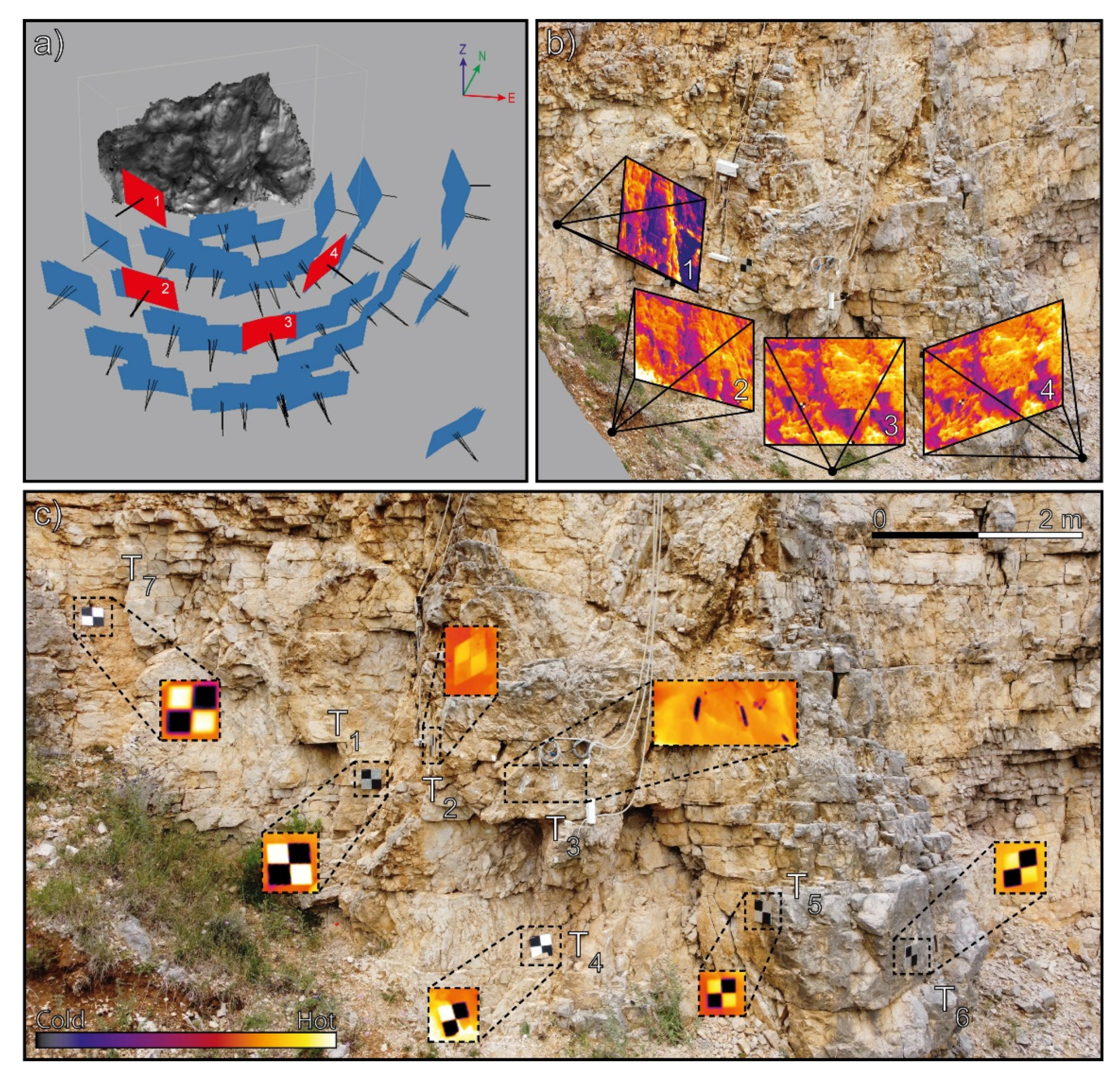
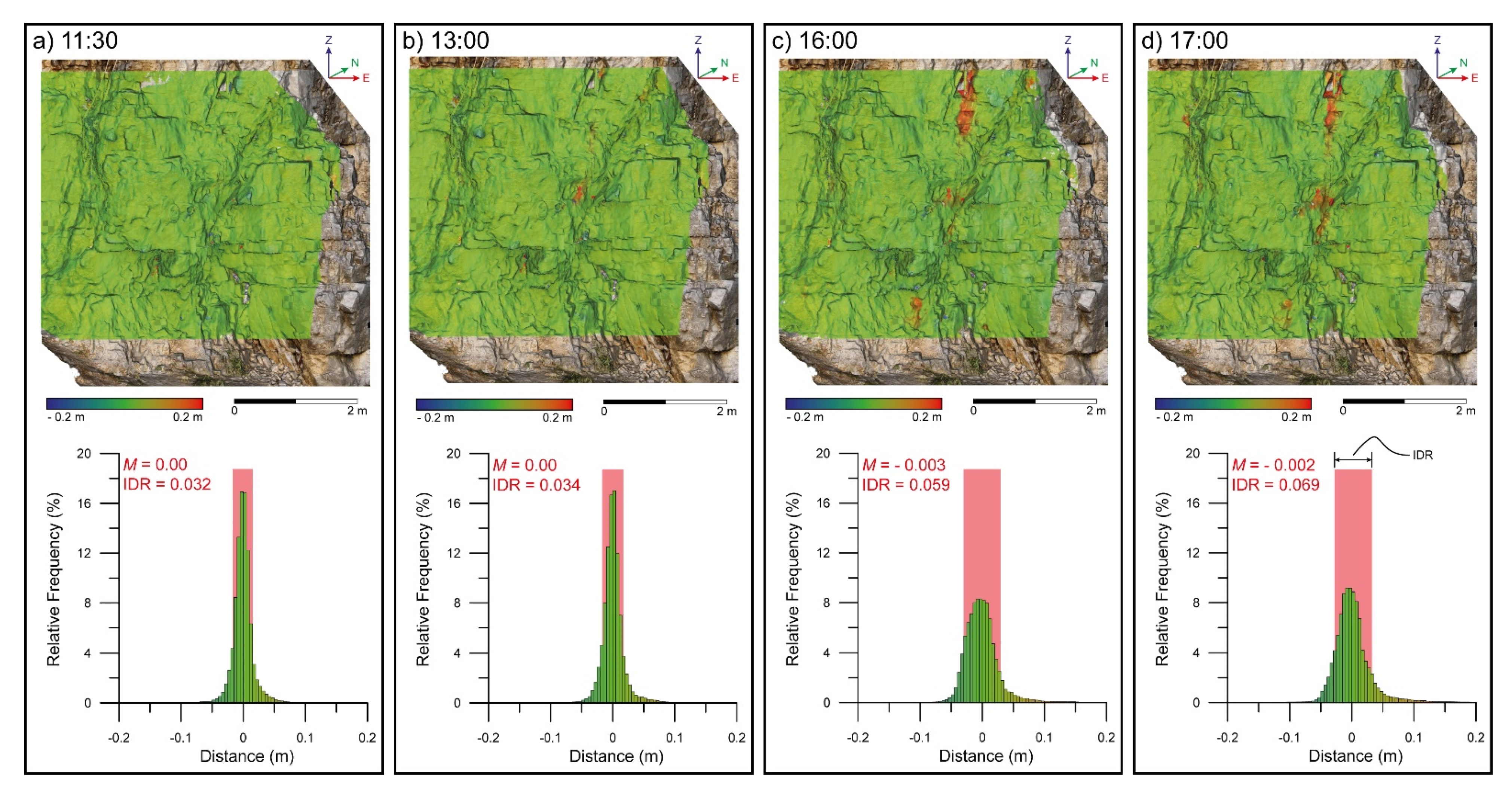
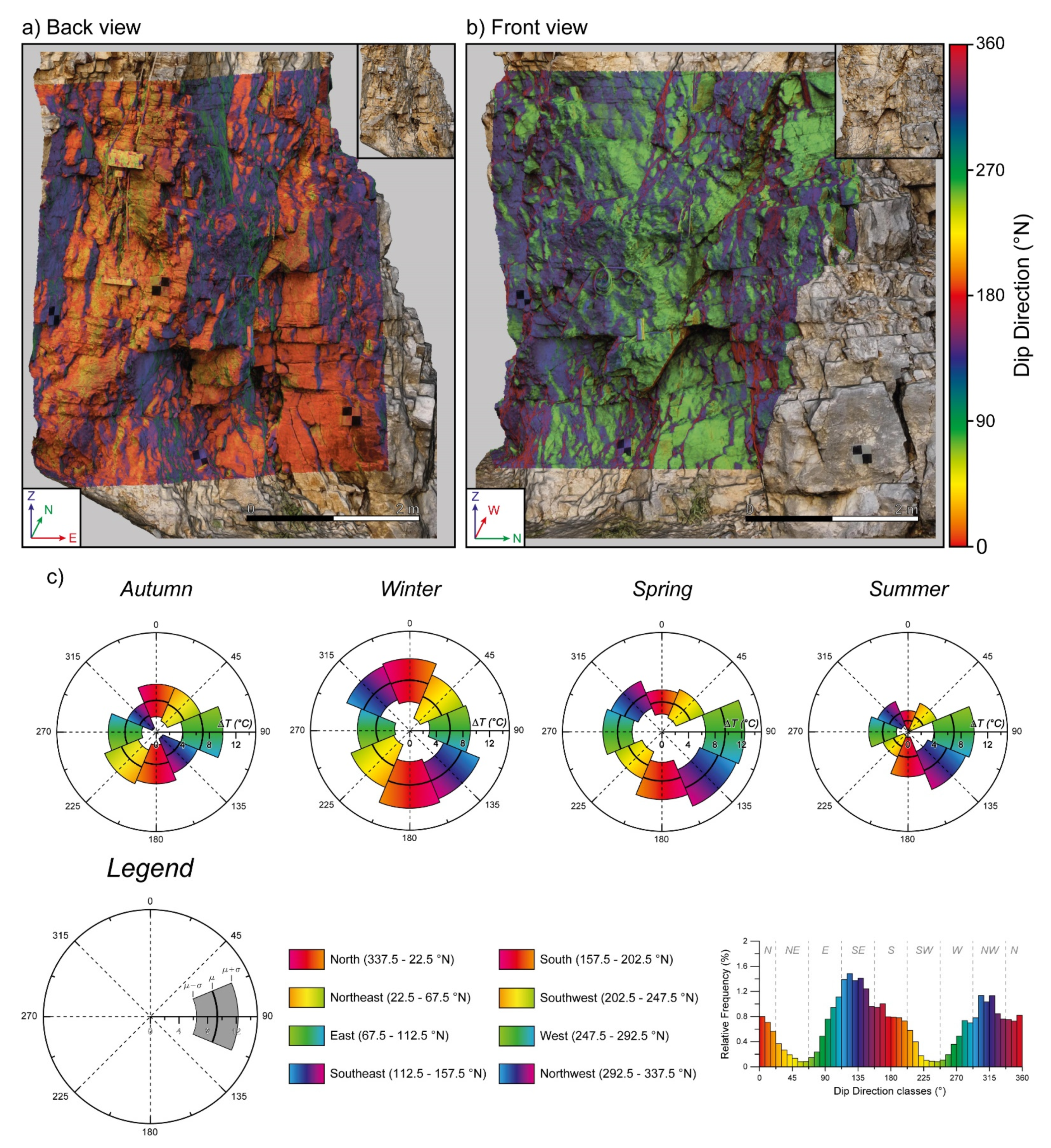
Table 1.
An example of the relation between the number of acquired photos during the IRT spring survey and number of points characterizing TIR sparse and dense point clouds.
Table 1.
An example of the relation between the number of acquired photos during the IRT spring survey and number of points characterizing TIR sparse and dense point clouds.
| Acquisition Time | No. of Photos | Sparse Points | Dense Points |
|---|---|---|---|
| 11:30 | 142 | 1.47 × 10⁴ | 2.87 × 10⁵ |
| 13:00 | 145 | 1.51 × 10⁴ | 3.17 × 10⁵ |
| 16:00 | 173 | 1.85 × 10⁴ | 3.83 × 10⁵ |
| 17:00 | 181 | 2.33 × 10⁴ | 3.89 × 10⁵ |
Publisher’s Note: MDPI stays neutral with regard to jurisdictional claims in published maps and institutional affiliations. |
© 2021 by the authors. Licensee MDPI, Basel, Switzerland. This article is an open access article distributed under the terms and conditions of the Creative Commons Attribution (CC BY) license (http://creativecommons.org/licenses/by/4.0/).
Share and Cite
MDPI and ACS Style
Grechi, G.; Fiorucci, M.; Marmoni, G.M.; Martino, S. 3D Thermal Monitoring of Jointed Rock Masses through Infrared Thermography and Photogrammetry. Remote Sens. 2021, 13, 957. https://0-doi-org.brum.beds.ac.uk/10.3390/rs13050957
AMA Style
Grechi G, Fiorucci M, Marmoni GM, Martino S. 3D Thermal Monitoring of Jointed Rock Masses through Infrared Thermography and Photogrammetry. Remote Sensing. 2021; 13(5):957. https://0-doi-org.brum.beds.ac.uk/10.3390/rs13050957
Chicago/Turabian StyleGrechi, Guglielmo, Matteo Fiorucci, Gian Marco Marmoni, and Salvatore Martino. 2021. "3D Thermal Monitoring of Jointed Rock Masses through Infrared Thermography and Photogrammetry" Remote Sensing 13, no. 5: 957. https://0-doi-org.brum.beds.ac.uk/10.3390/rs13050957
Note that from the first issue of 2016, this journal uses article numbers instead of page numbers. See further details here.