
Feasibility Analysis of GNSS-Reflectometry for Monitoring Coastal Hazards


1
School of Civil and Construction Engineering, Oregon State University, Corvallis, OR 97331, USA
2
Marine Science and Convergence Engineering, Hanyang University, Ansan 15588, Gyeonggi-do, Korea
*
Author to whom correspondence should be addressed.
Remote Sens. 2021, 13(5), 976; https://0-doi-org.brum.beds.ac.uk/10.3390/rs13050976
Submission received: 29 December 2020
/
Revised: 23 February 2021
/
Accepted: 24 February 2021
/
Published: 4 March 2021
(This article belongs to the Special Issue GNSS for Geosciences)
Abstract
:Coastal hazards, such as a tsunamis and storm surges, are a critical threat to coastal communities that lead to significant loss of lives and properties. To mitigate their impact, event-driven water level changes should be properly monitored. A tide gauge is one of the conventional water level measurement sensors. Still, alternative measurement systems can be needed to compensate for the role of tide gauge for contingency (e.g., broken and absence, etc.). Global Navigation Satellite System (GNSS) is an emerging water level measurement sensor that processes multipath signals reflected by the water surface that is referred to as GNSS-Reflectometry (GNSS-R). In this study, we adopted the GNSS-R technique to monitor tsunamis and storm surges by analyzing event-driven water level changes. To detect the extreme change of water level, enhanced GNSS-R data processing methods were applied which included the utilization of multi-band GNSS signals, determination of optimal processing window, and Kalman filtering for height rate determination. The impact of coastal hazards on water level retrievals was assessed by computing the confidence level of retrieval (CLR) that was computed based on probability of dominant peak representing the roughness of the water surface. The proposed approach was validated by two tsunami events, induced by 2012 Haida Gwaii earthquake and 2015 Chile earthquake, and two storm surge events, induced by 2017 Hurricane Harvey and occurred in Alaska in 2019. The proposed method successfully retrieved the water levels during the storm surge in both cases with the high correlation coefficients with the nearby tide gauge, 0.944, 0.933, 0.987, and 0.957, respectively. In addition, CLRs of four events are distinctive to the type of coastal events. It is confirmed that the tsunami causes the CLR deduction, while for the storm surges, GNSS-R keep high CLR during the event. These results are possibly used as an indicator of each event in terms of storm surge level and tsunami arrival time. This study shows that the proposed approach of GNSS-R based water level retrieval is feasible to monitor coastal hazards that are tsunamis and storm surges, and it can be a promising tool for investigating the coastal hazards to mitigate their impact and for a better decision making.
1. Introduction
Extreme waves such as tsunamis and storm surges have severely damaged coastal communities, including casualties and property losses. The various countermeasures could not have protected the coastal communities perfectly every time. For this reason, the monitoring techniques have been developed for early warning and post-event analysis.
Tsunamis generated by submarine earthquakes, landslides, volcanic eruptions, and meteorites cause a severe threat to coastal communities [1]. Consequently, it is crucial to understand the physics of tsunamis and apply our knowledge to tsunami early warning, hazard assessment, and mitigation tools to reduce tsunamis’ damage [2]. To understand the generation, propagation, and run-up of tsunamis, the in-depth analysis of recent and historical tsunami studies is essential [2].
A tsunami can be investigated either by observing in real-time or analyzing after the tsunami attacks the coastal cities, which is referred to as the post-tsunami survey. The real time observation is vital to tsunami warning centers for confirming the generation of tsunamis and predicting the potential locations of coastal communities to be damaged. Several tsunami observation networks are now in operation throughout the world. The representative tsunami observation networks are Deep-Ocean Assessment and Reporting of Tsunamis (hereafter called DART) system and Dense Oceanfloor Network System for Earthquakes and Tsunamis (hereafter called DONET), which are operated by NOAA and Japan, respectively. The DART system consists of a bottom pressure recorder (hereafter called BPR) and a surface buoy. Sea level measurements by BPR are transmitted to surface buoy via underwater acoustic communication and then to the tsunami warning center through satellite. The DONET system includes several nodes that are connected by fiber optic cables. Each node contains seismometers, bottom pressure recorders, and hydrophones, etc. [3]. These networks are installed in the open ocean for direct measurements of tsunami waves. Tsunami warning centers provide more accurate tsunami forecasting, including information about tsunami propagation and inundation using observed data [4]. These global observations of tsunamis also contribute to the historical tsunami databases of the National Center for Environmental Information and World Data Service, improving our knowledge of tsunami physics and developing the mitigation tools and programs to reduce damage from future tsunamis [5].
The post-tsunami survey has been performed by in situ expeditions soon after tsunami hits coastal communities [6]. The post-tsunami survey mainly collects data of inundation distance, tsunami heights/flow depths by filed inspections (e.g., splash marks left on the building, scratches in the bark, and broken twigs identified in a tree), and interviews of eyewitnesses to generate a tsunami inundation map in broad coverage of affected locations along the coastline [7,8]. The post-tsunami survey significantly contribute to historical tsunami databases [5].
As a part of tsunami observation instruments, coastal tide gauges have been used for measuring low-frequency wave components, primarily tide [6]. The role of coastal tide gauges for tsunami detection is to strike the tsunami on a specific area and assess its impact with respect to the arrival time and scale. Therefore, the tide gauge observations can be used to warn other coastal communities where the tsunami takes more time to reach. After the tsunami strikes coastal cities, the observation is used for defining tsunami initial waveform, its arrival time, and maximum tsunami wave heights.
Storm surges also are monitored by observation instruments, including tide gauge. Wind-driven storms are one of the major coastal hazards in the world, as well as tsunamis. Storm surges accompanied by a storm cause an abnormal sea-level rise induced by wind stress and sea-surface pressure gradient [9]. These also cause critical inundation to coastal areas. For instance, the storm surge height induced by tropical cyclone Mahina was 13 m in North Queensland in 1899 [10].
The frequency of storm surges has typical periods from several hours to approximately one week [11] and has much longer periods than tsunamis, ranging from one to two minutes up to about 3 hours [12]. Although these coastal hazards have different frequencies, as mentioned above, both tsunamis and storm surges can cause inundation and destructive damage to coastal communities [9].
To reduce casualties and property damages from tsunamis and storm surges, the event driven water level changes should be precisely measured. As mentioned above, a direct measurement by tide gauges is commonly used to investigate and analyze those events.
However, tide gauges, which are equally used for monitoring tsunamis and storm surges, can be destroyed by these coastal events. Becides, a prompt post-tsunami survey is critical because the site can be cleaned up and reconstruction. It is also not reliable as time passes (e.g., interviews of eyewitnesses) [7,13]. Recently, a new method of measuring water level variations using Global Navigation Satellite System (GNSS) was introduced [14], which is referred to as GNSS-Reflectometry (GNSS-R). Unlike a tide gauge, GNSS-R detects the distance between a GNSS antenna and the water surface through a remote sensing technique that allows indirect measurements of water level variations over time. As this method must be less vulnerable to coastal hazards because of the remote sensing concept, it can be useful not only for monitoring coastal hazards, but also for continuously measuring water level throughout the period of coastal hazards.
This study introduces GNSS-Reflectometry (GNSS-R) as a remote sensing technique for the post-analysis of extreme events such as tsunami arrival time and storm surge level in Section 2. The GNSS-R was applied to analyze the water level fluctuation during the tsunami and hurricane events. The results were compared with the tide gauge data in Section 3 and Section 4. Through the results, the conclusion and discussion were described in Section 5 and Section 6.
2. GNSS-Reflectometry for Extreme Coastal Events
2.1. GNSS-R Rased Water Level Measurements
Most signals arriving at a GNSS antenna are received directly through their line of sight, but some of them are received after one or multiple reflections from the surrounding terrains or obstacles. The signals received after the reflection are known as multipath. When the receiver receives the reflected signals, a notable interference pattern on signal-to-noise ratio (SNR) data occurs. Larson et al. (2008) presented the SNR by
where and are the amplitudes of direct and multipath signals, respectively, and is the phase difference between two signals [15].
Since the multipath is considered one of the error sources for GNSS positioning, the receivers and antennas are designed to mitigate the impact of multipath. In addition, the signals tend to be attenuated after the reflection. Therefore, [16] approximated the SNR by
The above equation implies that the amplitude of the multipath signals of SNR is smaller than the one from the direct signal. Additionally, the multipath oscillates in a single data span, while the direct signal goes through a complete cycle only once over a satellite pass [15]. Consequently, the contribution of the multipath on SNR data can be isolated by removing the main trend using a second-order polynomial function.
Assuming a planar reflector, the phase differences between the direct and reflected signals can be modeled by the geometric relationship between a satellite, an antenna, and a reflector.
where is the wavelength of a GNSS signal, is the additional path delay of the reflected signal, is the satellite elevation angle, and h is the antenna height above the water surface. By taking a derivative of the phase of the dSNR with respect to the sine of the elevation angle, the linear relationship between the frequency () of the oscillation and the height () above the reflecting surface can be derived.
With the linear relationship, the frequency of the oscillation can be identified by a spectral analysis using the detrended SNR data that can be converted to the antenna height. However, this approach assumes that the reflector height is not time-dependent during a certain period of time, which is not realistic, because the actual water level continuously changes. Since this model is not sufficient for the sites with high tidal variations and with a strong meteorological forcing, Larson et al. (2013) introduced correction terms for the variation of antenna heights and satellite elevation angles changing over time [17].
where and define the velocity of antenna height above the water surface and the satellite elevation angle, respectively; is the antenna height considering the water level variations, called the kinematic height in this study. By introducing the antenna height computed based on the static assumption, , the same form as Equation (4) is acquired, which can be continuously converted to the linear relationship between the frequency of the oscillations and antenna height.
Tropospheric effect is one of signal propagation errors occurring due to the tropospheric effect. It is highly correlated with the geometry between a satellite and a receiver, as well as the location of receiver. Therefore, the tropospheric delay is considered as a geometry term in the GNSS observations. In the early works on sea level estimation using GNSS-R based tide gauge, Williams and Nievinski (2017) investigated the tropospheric effect on the GNSS-R based water level measurements by using more than 20 GNSS coastal sites and found that ignoring the tropospheric delay induces a manifest scale error in the reflector heights [20]. They estimated the effect of the tropospheric delay and revealed that the tidal coefficients were smaller than the true amplitudes by about 2% (2 cm/m) without the tropospheric correction. Accordingly, they strongly recommended the correction of the tropospheric delay in GNSS-R for sea level studies.
The troposphere can be separated into dry and wet components. The dry and wet delays can be modeled at zenith direction of a receiver, which should be properly projected onto the ray path between a satellite and a receiver by
where is the tropospheric delay along the line of sight, is the zenith delay difference across antenna and surface positions, and mh and mw are the mapping functions for hydrostatic and wet components, respectively. The antenna height delay () caused by the tropospheric delay () can be obtained from a derivation of the tropospheric delay with respect to the sine of the elevation angle.
In this study, the dry and wet tropospheric effects along the zenith direction are computed using UNB3 model [21] developed based on Saastamoinen model [22], which is one of the most reliable models [23]. UNB3 model uses the predicted meteorological parameters from a lookup table embedded in the model that provides more realistic meteorological values than a set of constant values, such as standard atmospheric parameters. For the projection, a Global Mapping Function (GMF), suggested by Boehm et al. (2006), is applied [24]. The GMF is developed based on the Vienna mapping function (VMF) that is widely known as the most accurate mapping function. However, unlike the VMF, the GMF does not require the meteorological data and determines its coefficients based on data from the global ECMWF (European Centre for Medium-Range Weather Forecasts) numerical weather model.
2.2. Enhanced GNSS-R Based Tide Gauge for Extreme Coastal Events
Although the time-dependent correction term, in Equation (5), is added as a dynamic reflector height, the method described in Section 2.1 requires processing a significant portion of each line of sight satellite observations to retrieve the reflector height measurement. Accordingly, the sea level retrievals from the GNSS-R algorithms in Section 2.1 are not sufficient for extreme coastal events that require high precision with high temporal solution. In this section, we introduce the enhanced GNSS-R data processing algorithms to detect the extreme coastal events.
To effectively investigate the sea level variations with high temporal resolution, the frequency of the multipath oscillation, that is f in Equation (6), is determined using the detrended SNR data based on a sliding window. The optimal sliding window is defined by determining the sliding interval and window width. First, the sliding interval can be reduced to the data sampling rate, and the application of a small sliding interval allows the GNSS-R-based tide gauge to monitor the water level change with high temporal resolution. However, defining the width of window is not as simple as the sliding interval. The window width should be large enough to extract the multipath effect from the water surface, but not too large to monitor for rapid changes in water level during severe weather events. To quantitatively determine the appropriate window width, priori knowledge of the minimum and maximum antenna height above the water surface is utilized [16]. Roussel et al., 2015, estimated the expected frequency of the oscillations (, ) from minimum and maximum antenna height (, ) based on the Equation (5) considering the kinematic antenna height. However, in this study, we ignored the height variations during the period of the processing window for determination of the optimal window in order to minimize the computational workload. Instead, we considered the minimally sufficient length of signals that allows the spectral analysis for retrieving the reflector height and still secures the high temporal resolution of output. Consequently, the window width should be determined within the range below.
where is the window width and is the number of oscillation cycles on SNR data due to multipath. Finally, the optimal window width is determined as below.
According to the linear relationship in Equation (6), the antenna height above the water surface is directly converted from the frequency derived by a spectral analysis using the detrended SNR signal. Therefore, the reliable determination of the frequency associated with the multipath from the water surface, referred to as a dominant frequency, is crucial for a precise water level determination. To derive this frequency, Lomb Scargle Periodogram (LSP) is applied, which allows the spectral analysis of uneven sampling data. Yet, the determination of the dominant frequency for the multipath oscillations is not straightforward because of the roughness of the water surface and the time-varying parameters such as , in Equation (6), especially during extreme weather conditions with the high currents and strong wind. To avoid the pitfall of selecting a wrong frequency, we take an advantage of the multi-band GNSS signals. Under GNSS modernization, most GNSS satellites transmit dual or multiple bands of signal; especially, Galileo transmits five band signals, E1, E6, E5, E5a, and E5b. These multiple band signals transmitted from the same satellite travel through the same ray path; thus, the resulting heights of a specular point computed by all signals is expected to be consistent. Consequently, our approach inspects the heights derived by a dominant peak from multi-frequency bands of a single ray path, then examines the consistency between them. If the resulting heights from multi-band signals on a single ray are inconsistent within a certain threshold, the algorithm sets the most reliable height based on the power of the candidate peaks. Based on this, the less reliable heights are re-defined by performing cross-check with multi-band signals.
Once the frequency of the oscillation is correctly determined for each ray path, the static antenna height () can be obtained by Equation (5). Then, the height (h) and the height rate () are combined, which are presented in [16] and [25]. Roussel et al., 2015, introduced the method to conjointly estimate the height and the height rate by combination of the measurements from all the available GNSS satellites insight at a given epoch using a classical LSM [16]. Wang et al., 2019, improved the algorithm by considering errors caused by water level fluctuation and atmospheric refraction and estimated the parameters through a robust regression strategy [25]. In this study, the unknown parameter estimation is conducted by a Kalman filter method, which recursively estimates the unknown parameters at the current epoch based on the parameters estimated at the previous epoch. As the Kalman filter is the one of the powerful estimation algorithms widely applied in various fields, we have omitted the basic concept of the Kalan filter. Instead, the system of the Kalman filter applied in this study is summarized in Equation (12). Through the Kalman filter, the kinematic height, H, and the height rate, , can be conjointly estimated with the consideration of the tropospheric effect computed by Equation (8).
where and are the state and measurement vector at epoch k, respectively. is a design matrix a. In the design matrix, is newly introduced, which is the time difference between the epoch of measurement i and the target epoch k. With the corresponding system, the Kalman filter recursively estimates the unknown parameter by applying the estimation results and uncertainly from the previous epoch. As the initial information is required for the first epoch, we adopted the LESS for computing the initial information. More detailed information about the system of state transition equation for the combination can be found from Wang et al., 2019 [25]. In addition, the basic concept and more information on the Kalman filter can be found from Kalman 1960 [26].
3. Water Level Estimation during Tsunamis in 2012 and 2015
To verify the feasibility of GNSS-R for monitoring tsunamis, two tsunami events were analyzed that were induced by 2012 Haida Gwaii earthquake and 2015 Chile earthquake. Based on the event record of the NOAA center for Tsunami Research (https://nctr.pmel.noaa.gov/, accessed on 1 March 2021), the effects of the two tsunamis were observed by a tide gauge in Crescent City, CA, which is NOAA National Water Level Observation Network (NWLON) sentinel station (ID: 9419750). The detailed information about the events can be found from the subsections.
An NGS CORS (Continuously Operating Reference Stations), CACC, is located right next to the NOAA tide gauge (ID: 9419750), which has a clear and wide-open view toward the ocean covering the north and west side from the antenna. The equipment at this site consists of Trimble 57971 Zephyr Geodetic antenna and a Trimble NetR9 receiver, which records GPS and GLONASS signals with 30 s of sampling interval. Note that CACC recorded only dual-frequency signals until 2013 and began recording triple-frequency signals from 2014. In the experiments in Section 3.1 and Section 3.2, all available signals at CACC were processed for the tsunami analysis.
As shown in Figure 1, obstacles such as small buildings exist near the antenna, which can lead to significant errors in water level computation due to the mixture of the signals reflected from multiple sources. To isolate the multipaths of the water surface from the other multipaths from these obstacles, the location of the reflector of each signal is computed using the orientation (azimuth and elevation angles) of the corresponding satellite from the antenna based on the first Fresnel zone (FFZ). In this experiment, we used the open source software package, GNSS interferometric reflectometry (GNSS-IR) [27], to investigate the appropriate range of the azimuth and elevation angles for the area of the water surface. In case of CACC, the satellite azimuth angles between −125° and 30° and the elevation angles between 0° and 45° were selected, shown as a map in Figure 2.
3.1. 2012 Haida Gwaii Earthquake
On 28 October 2012 (03:04:08 UTC), a magnitude 7.8 earthquake (52.788 °N, 132.101 °W) occurred at the Queen Charlotte Islands in Canada. A tsunami generated by this earthquake was non-destructive and measured throughout the Pacific, including Alaska to California, and Hawaii. Based on the event record of the NOAA center for Tsunami Research (https://nctr.pmel.noaa.gov/ (accessed on 1 March 2021)), a tide gauge located on Crescent city (ID: 9419750) recorded this tsunami. The arrival time at Crescent city was 2012-10-28 05:44 UTC, and the maximum wave height was 0.44 m.
In this study, we analyzed the SNR data from 15 October to 13 November at CACC station in Crescent City that covers the time period of the arrival of tsunami. The processing result was compared to the independently measured water levels by the co-located tide gauge. For the direct comparison of the water level measurements, vertical reference surfaces retrieved from two sensors should be synchronized, because the outputs from two sensors refer to different vertical datums. The GNSS-R based tide gauge refers to geodetic datum, while the tide gauge refers to localized tidal datum. For the datum synchronization, the difference between the geodetic and tidal local datums at CACC was computed using NOAA’s vertical datum transformation tool, VDatum (https://vdatum.noaa.gov/about.html (accessed on 1 March 2021)). As the difference between two datums was 1.015 m, they were synchronized by shifting one dataset to another.
Figure 3 shows the water levels derived by GNSS-R based tide gauge (red dots) and the conventional tide gauge (blue dots). The GNSS-R measurements are the heights retrieved by Kalman filter by considering the height rate. From the corresponding time-series plot, it was confirmed that the GNSS-R technique successfully estimated the water level variation, because it shows a good agreement with the co-located tide gauge even during the period of the tsunami event.
For numerical comparison, the correlation coefficient (CC) between the water level measurements from GNSS-R based tide gauge and the tide gauge were computed in Figure 4. The sea level measurements of the tide gauge were interpolated to the time tag of the GNSS-R measurements, and the CC of static tide was computed. As a result, comparable high CC of 0.944 were computed, which demonstrates the performance of the GNSS-R-based tide gauge. In addition, we assessed the impact of the tsunami event on CC. During the period of the tsunami event (Oct 28 05:44–Oct 29 12:00), the CC of the water level extracted from the GNSS-R measurements was calculated as 0.920. Although they still show a considerably high correlation, the performance of the GNSS-R was degraded due to the tsunami event.
The water level differences between the sea level measurements from the GNSS-R based tide gauge and the co-located tide gauge were computed in Table 1. The mean difference was computed as 0.189 m with RMS of 0.230 m. In addition, the differences in the tsunami event were calculated and compared with those calculated using the measurement from the entire period. As with the analysis using CC, the degradation of the GNSS-R based tide gauge due to the tsunami was identified.
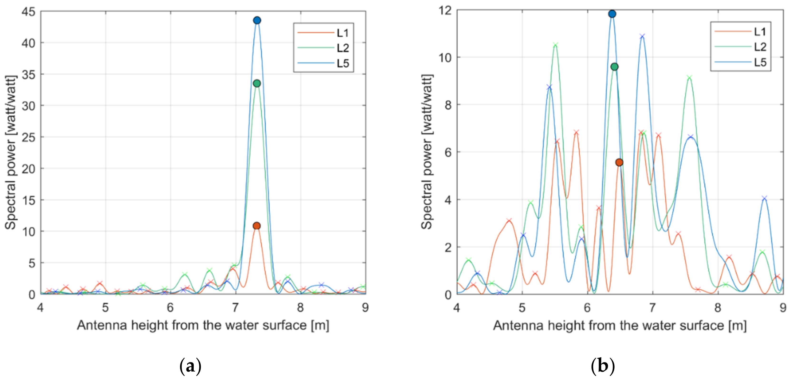
For the further investigation on the effect of the tsunami, we examined performance of the dominant frequency detection process during the event. As aforementioned, the SNR data should be converted to the spectral domain, which returns multiple frequencies, and water levels are directly computed from the most dominant frequency. However, the sea surface is not the normal condition during extreme events, especially tsunamis. Therefore, determining a dominant frequency representing a water surface during a certain time window during tsunamis is certainly challenging. Figure 5 is the processing results of the triple band of the same satellite (GPS PRN01) during calm and normal condition (left) and during a tsunami event (right). As shown in the left plot, we can distinctly detect a dominant height during the calm water surface, and the heights from different band signals (L1, L2, and L5) indicate the same antenna heights, 7.3 m. However, during the rough sea surface, one dominant height cannot be easily determined, as three bands signals point to different heights. One possible interpretation of this is due to the unstable water surface affected by the tsunami wave that interrupts, retrieving one representing reflector surface. In the plot, a dominant peak from the signal from each band was selected through the algorithm described in Section 2.2. Although the algorithm still enables selecting height from multi-band signals, it is evident that the heights converted from them are less reliable. In addition, the heights calculated from the dominant peaks of the triple frequency signals are not aligned as much as the heights computed during the calm condition.
As shown in Figure 3b, a tsunami significantly degraded the performance of water level retrieval using GNSS-R. To assess the impact of the event on the sea levels, we introduced a numerical indicator, Confidence Level of Retrieval (CLR), by calculating the amplitude of the dominant peak with respect to the other remaining peaks. The CLR provides an intuitive understanding about the superiority of the dominant peak with respect to the remaining peaks.
where is the power of the peak marked as dominant; is the power of the other remaining peaks. The CLR was computed during the entire processing period, the results of which are provided as the time series in the top plot in Figure 6.
To clearly identify the duration of the 2012 Canada tsunami in Crescent city, CA, the tsunami components were extracted from sea levels from the tide gauge. The tsunami component was derived through a phase-preserving high-pass Butterworth filter (cutoff period: 4 h; the order: 4) [28]. As shown in the bottom plot of Figure 6, we estimated the period (Oct 28 05:44–Oct 29 12:00) of the tsunami effect in Crescent city, CA. From the comparison between these plots, it was confirmed that the CLR rapidly declined right after the tsunami arrival time and then gradually recovered as the tsunami impact was attenuated. Prior to the arrival of the tsunami, the average CLR was calculated at 7.512, but the average CLR during the tsunami event was 3.979, which means there was 47% of deduction due to the tsunami.
3.2. 2015 Illapel Earthquake
The 2015 Chile tsunami was generated by a magnitude 8.3 Central Chilean earthquake (31.570° S, 71.654° W) on September 16, 2015 (22:55:26 UTC). The tsunami propagated all over the Pacific region and was observed by NOAA tide gauge in Crescent City (ID: 9419750). According to the NOAA Center for tsunami research, this tsunami arrived at Crescent City at September 17, 2015, at 13:39 UTC with 0.32 m maximum wave heights.
We processed the SNR data collected at CACC in Crescent City, CA for one month in September 2015. For the validation of GNSS-R based tide gauge using the cooperating traditional tide gauge, we applied the same vertical datum offset between these two sensors obtained from VDatum as the experiment of 2012 Canada tsunami (Section 3.1). Figure 7 shows the time series of the water level measurements of the GNSS-R based tide gauge estimated by the Kalman filter in Crescent City, CA, with additional magnification plots during normal condition and the tsunami event. Overall, the sea level measurements from GNSS-R based tide gauge are very close to those of the tide gauge. In particular, even after the tsunami arrival, the GNSS-R based tide gauge was able to successfully estimate the sea levels.
The CC results in Figure 8 also show the successful performance of the GNSS-R based tide gauge as we confirmed through the time-series analysis. The CC of 0.933 was calculated using the GNSS-R measurements for the entire processing period, and 0.930 was calculated using only measurements during the event period. From the corresponding results, we confirmed that the GNSS-R based tide gauge was able to estimate the sea levels regardless of the tsunami event. The statistical analysis results of sea level differences between GNSS-R-based and cooperative tide gauge showed even smaller differences during the tsunami period (Table 2). The mean differences were computed as 0.201 and 0.144 m, respectively, during the entire period and the tsunami period.
Furthermore, the CLR was computed using the SNR data for the entire processing period, which was compared with the tsunami component in the sea level measurements the tide gauge processed by a phase-preserving high-pass Butterworth filter (cutoff period: 4 h; the order: 4) [28]. The time-series of the tsunami components in Figure 9 (bottom plot) clearly shows that the 2015 Chile tsunami had a significant impact on sea level changes right after the arrival of the tsunami, and this effect lasted about three days (red box in the plot). In addition, the secondary impact of the tsunami also was detected in both sensors around September 24, which is shown in the blue box. Similar to the 2012 tsunami case study in 3.1, the CLR rapidly declined after the arrival of the tsunami, and then gradually recovered as the tsunami effect disappeared. The average CLRs were calculated as 9.998 and 4.065 before the arrival of the 2015 Chile tsunami and during the period of the tsunami (from 13:39 on September 17 to 3:00 on September 20), respectively, which indicates the 59% of deduction caused by the tsunami. In addition, this pattern in CLR was clearly confirmed in the second impact of the tsunami indicated by the blue box in the figure.
4. Water Level Estimation during Storm Surges
4.1. Hurricane Harvey in 2017
Hurricanes lead one of the catastrophic coastal hazards. In 2017, Hurricane Harvey caused insured loss of $125 billion and maximum inundation levels of 6 to 10 ft above ground level in Texas and Louisiana due to the combined effect of the surge and tide (NOAA, 2017). In this study, we utilized our GNSS-R method for monitoring a storm surge caused by Hurricane Harvey. We processed SNR data collected at CALC, which was one of NGS’s CORS, and compared them with the tide measurements from co-located tide gauge. The CALC station and the tide gauge are installed on the same NWLON sentinel station (station ID: 8768094) in Cameron, LA, which Harvey passed between 30–31 August, 2017. Trimble 57971 Zephyr GNSS Geodetic II antenna and a Trimble NetR9 receiver are installed at the CALC station, which collects multi-GNSS constellations data including GPS, GLONASS, and Galileo and archives them with 30 s of sampling rate. As shown in Figure 10, this site has open view toward the ocean in all directions. Consequently, GNSS signals from all satellite azimuth angles (0–360°) and elevation angles between 0° and 90° were selected for the sea level estimation through FFZ computation using GNSS-IR software.
The sea level measurements from GNSS-R based tide gauge were validated with the traditional tide gauge after compensating the vertical datum offset, 12.8 cm from the VDatum. In addition, further adjustment between two measurements were computed and applied after the VDatum correction, which possibly proceeded from the systematic error of the sensors or the VDatum. By considering the period of the Harvey, we analyzed the SNR data from August 14 to September 7 in 2017 at CALC station in Cameron, LA. Figure 11 shows the time series plot of the sea levels estimated by the GNSS-R based tide gauge (red dots) and the co-located tide gauge (blue dots). Note that the sea level measurements from GNSS-R based tide gauge are the kinematic heights that include the height rate during Kalman filtering. This plot clearly shows that the GNSS-R based tide gauge shows a good agreement with the tide gauge measurements over the entire processing period. The CCs between the sea levels derived from GNSS-R based tide gauge and the tide gauge are provided in Figure 12. Extremely high correlation of 0.987 was obtained by using the GNSS-R results during the entire processing period. For the assessment of impact of the storm surge on the sea level measurements of GNSS-R based tide gauge, the CC during the event period (Aug 24 at 12:00–Aug 30 at 24:00) was additionally computed. The period of the event was detected by analyzing the tide gauge measurements through the high-pass filter extracting the storm surge components (Figure 13 (bottom)). As a result, CC of 0.972 was obtained during the event, which proves that GNSS-R based tide gauge can monitor the storm surge with very high performance.
Table 3 provides the statistical analysis results of the water level differences between GNSS-R based tide gauge and the co-operating tide gauge. Using the sea levels during the entire processing period, the mean differences were computed as 0.027 m with the RMS of 0.038 m. During the event, the mean and RMS of the sea level differences were 0.037 and 0.055 m, respectively.
Figure 13 compares the CLR changes with the storm surge components extracted from the sea level measurements of the tide gauge. The average CLRs were calculated as 7.953 and 6.094 before and during the period of the storm surge, respectively, which indicates the 23% of deduction caused by the storm surge. Although the storm surge degraded the reliability of signal retrieval, the impact from the storm surge was much less compared with the two tsunami cases in Section 3.1 and Section 3.2, where the CLR deductions from the tsunamis were 47% and 59%.
4.2. Storm Surge in Alaska in 2019
On February 12, 2019, there was a coastal storm surge in the western coast of Alaska that caused severe flooding. Waves transported an enormous ice berm, and a snow berm was positioned at flooding coastal areas. In this study, we processed SNR data collected at AT01 CORS in St. Michael, Alaska, from January 26 to February 19 to monitor the water level variation during the storm surge. AT01 is one of PBO network stations operated by UNAVCO, which is primarily designed to investigate the feasibility of the GNSS-R based tide gauge. This site has a clear and open view toward the sea as shown in Figure 14, and the most effective azimuth (0–230°) and elevation (10–25°) ranges are given. The FFZ were computed using the given azimuth and elevation angles, as shown in the enlarged map in Figure 14; all FFZ were located on the water surface. The equipment at this site consists of a Trimble 159800 Choke Ring antenna and a Septentrio PolaRx5 receiver that can receive GPS, GLONASS, Galileo, and BeiDou signals. The performance of AT01 was also evaluated and verified by Kim and Park (2019). They achieved a high correlation coefficient of 0.87 with the sea level measurements for the closest tide gauge. For the experiment, we processed all available multi-GNSS signals, and the results were validated using the tide gauge station located about 74 km away from the AT01 as a ground truth that was the nearest tide gauge from AT01. This tide gauge is one of NWLON sentinel stations operated by NOAA in Unalakleet on the western coast of Alaska.
As described in the earlier section, the vertical datum offset between the GNSS-R based tide gauge and the conventional tide gauge should be eliminated based on the datum conversion with respect to the tidal datum. However, there are significant gaps in the coverage of vertical datum in Alaska due to insufficient number of operating tide gauges so that VDatum does not provide the information for the datum conversion. Instead, we computed and applied the averages of the vertical differences (0.316 m) to the time series for comparisons.
Figure 15 shows the sea levels derived by the GNSS-R base tide gauge (red dots) in St. Michael compared with the sea level measurements from the tide gauge (blue dots) in Unalakleet. Overall, the GNSS-R based tide gauge shows a good agreement with the traditional tide gauge. However, the time-series plot also indicates slight inconsistency especially during the period of the storm surge, which can be explained by the distance between two sensors.
For quantitative investigation of agreement between these two measurements, the CC was computed during the entire processing period and the period of the storm surge in Figure 16. As a result, high correlation of 0.957 was observed when using the sea level measurements over the entire processing period, but the correlation was deteriorated to 0.868 when the storm surge occurred. Note that this site showed the lower CC than previous case studies because of the distance between the GNSS site and the tide gauge. The corresponding results were also confirmed through the statistical analysis of the water level differences between the GNSS-R based tide gauge and the tide gauge. The mean difference was computed as 0.140 m using the sea levels derived during the entire period, and when the storm surge occurred, the mean difference was increased to 0.410 m (Table 4). Again, the absolute distance between two sensors, which is 74 km, must lead the greater discrepancy than previous case studies in Section 3.1, Section 3.2, and Section 4.1.
We also computed the CLR before and during the storm surge event. Similar to the case of hurricane Harvey in Section 4.1, Figure 17 showed less deduction of CLR. Indeed, the average CLR increased from 16.625 before the storm surge to 18.328 during the storm surge (00:00 February 12 to 12:00 February 13). These results show that this storm surge did not cause the performance degradation of the GNSS-R based tide gauge, so the previously identified discrepancy with the tide gauge result from the long distance between the two sensors.
5. Discussion
The present study showed the feasibility of GNSS-R for monitoring tsunamis and storm surges. The proposed study successfully detected the extreme change of water level caused by two distinctive types of coastal hazards. To monitor the events, we analyzed (1) the time series water level variation during the event and (2) the reliability of the water level retrieval by CLR. Although the overall performance of the water level retrieval was acceptable among all case studies here, each type of event responded differently to the water level retrieval and the CLR. In case of tsunamis, the performance of GNSS-R for the water level retrieval was degraded due to the roughness of the water surface and the waves from tsunamis. However, the proposed technique still successfully estimated the arrival time of tsunami by analyzing the CLR. The significant deduction of CLR indicates the low reliability of retrieved water level that can be considered as the tsunami arrival time. The tsunami arrival time based on the CRL was verified by the tsunami component from the conventional tide gauge measurements. In case of storm surges, GNSS-R results showed high CC with the tide gage data even during the storm event. Unlike the tsunami cases, the CLR during the storm surge events did not notably decrease, and consequently the retrieved water level during the storm surge was as reliable as during a normal condition of water surface.
These results may be affected by the relation between the size of the GNSS-R data processing window and the periods of tsunami and storm surge. As described in the introduction, the typical tsunami periods are from several minutes to 3 h, while the storm surge periods are typically longer than 3 h. Therefore, the window width of GNSS-R data (approximately 1 h or less depending on the satellite’s geometry) cannot retrieve one representing reflector surface due to the shorter fluctuation of the water surface due to a tsunami. In case of a storm surge, the window width used in this study may be short enough to extract the representative water surface, as a storm surge lead a long-term variation relative to a tsunami. Therefore, the suggested study can be applied to detect tsunamis by analyzing the CLR over time and to detect storm surges by observing the time series of water level measurements that makes the proposed approach applicable to distinguish one from another.
6. Summary and Conclusion
Predicting and monitoring tsunamis as well as analyzing post-tsunami events are essential for mitigating their impact on coastal communities. While offshore observation systems are used to predict and monitor tsunami arrivals for early warning, tide gauges are used to collect post-tsunami information such as arrival time and tsunami heights for post event analyses. A storm surge also is another coastal event that can cause an inundation and flooding. A tide gauge is one of the conventional water level measurement sensors, but alternative measurement systems can be needed to compensate the role of tide gauge for contingency (e.g., broken and absence, etc.). Additionally, tide gauges are installed near the coast. Therefore, they cannot measure inland inundation height, which is needed for the post-tsunami survey.
In this study, we propose a GNSS-R based tide gauge for the post-event analysis by taking an advantage of the remote-sensing nature of GNSS-R technique. We introduced the enhanced GNSS-R algorithms for monitoring extreme coastal events that require detecting water level variations with high temporal resolution and high precision. We utilized multi-band GNSS signals transmitted on the single ray path of each satellite. This approach improves the reliability of the water level measurements in that the less reliable heights are re-defined by cross-checking with multi-band signals. In addition, a sliding window was applied to the data processing for improving the temporal resolution. By defining the optimal size of the processing window, the minimally sufficient length of signals for the spectral analysis was processed that significantly improved the temporal resolution of output without losing the reliability of result. For detecting dynamic variation of water level, we conjointly estimated the height and the height rate together with a Kalman filter method to recursively estimate the unknown parameters based on the parameters estimated at the previous epoch.
For analyzing the water level variation during the extreme events, we introduced a numerical indicator, CLR, which assesses the impact of the costal events on the sea level variation. The CLR provides an intuitive understanding about the superiority of the dominant peak representing the multipath with respect to the other remaining peaks in the spectral domain of signal.
This technique was applied to both tsunami and storm surge cases. From the results, the following conclusion can be drawn:
- In normal wave condition, water level fluctuation estimated by GNSS-R showed a good agreement with that by tide gauge, showing correlation coefficients of 0.933 minimum and 0.987 maximum from 2015 tsunami and Harvey events, respectively.
- GNSS-R results for both 2012 and 2015 tsunami data showed that the time of CLR drop corresponds to the tsunami arrival time collected by tidal gauges. The CLR deductions from the tsunamis were confirmed to be 47% and 59%, respectively.
- For storm surge cases, GNSS-R results kept high CLR during the entire event of storm surge and showed a high correlation with tide gauge data. The CLR calculated from Harvey indicates only 23% of deduction caused by the storm surge. Even the storm surge in Alaska showed an average CLR increase from 16.625 to 18.328 before and after the storm surge, respectively.
- The CLR difference between tsunami and storm surge events may result from the GNSS-R data window width. The characteristic periods of the extreme events, shorter than the window width, possibly degrade the CLR.
Therefore, it is found that GNSS-R can provide information about the tsunami arrival time in the coastal cities with no tide gauge or extreme weather conditions. Future studies can include the inundation and flooding level by overland flow by tsunami or storm surge using GNSS-R. It is also worth considering the use of new low-cost and multi-constellation equipment as a way to strengthen the monitoring network [29,30].
Author Contributions
Introduction: E.L., S.-K.K., J.P., and S.S.; data curation: S.-K.K. and E.L.; the result: S.-K.K.; analysis of results: S.-K.K., J.P., and S.S.; writing—original draft preparation: S.-K.K. and E.L.; writing—review and editing: J.P. and S.S. All authors have read and agreed to the published version of the manuscript.
Funding
This research was funded by Korea Meteorological Institute, grant number KMI2018-02510, and was supported by the Brain Korea 21 plus program through the National Research Foundation (NRF) funded by the Ministry of Education of Korea.
Institutional Review Board Statement
Not applicable.
Informed Consent Statement
Not applicable.
Data Availability Statement
Not applicable.
Conflicts of Interest
The authors declare no conflict of interest.
References
- National Centers for Environmental Information. Available online: https://www.ngdc.noaa.gov/hazard/data/publications/tsunami-hazard-assessment-2015.pdf (accessed on 15 April 2020).
- Rabinovich, A.B.; Fritz, H.M.; Tanioka, Y.; Geist, E.L. Introduction to “Global Tsunami Science: Past and Future, Volume II”. Pure Appl. Geophys. 2017, 174, 2883–2889. [Google Scholar] [CrossRef] [Green Version]
- Lee, E.; Jung, T.; Shin, S. Numerical and Probabilistic Study on the Optimal Region for Tsunami Detection Instrument Deployment in the Eastern Sea of Korea. Appl. Sci. 2020, 10, 6071. [Google Scholar] [CrossRef]
- Rabinovich, A.B.; Eblé, M.C. Deep-Ocean Measurements of Tsunami Waves. Pure Appl. Geophys. 2015, 172, 3281–3312. [Google Scholar] [CrossRef]
- Kong, L. Post-Tsunami Field Surveys are Essential for Mitigating the Next Tsunami Disaster. Oceanography 2011, 24, 222–226. [Google Scholar] [CrossRef]
- Levin, B.; Nosov, M. Physics of Tsunamis; Springer: Dordrecht, The Netherlands, 2009; ISBN 9781402088551. [Google Scholar]
- Arcos, N.P.; Dunbar, P.K.; Stroker, K.J.; Kong, L.S.L. The Impact of Post-tsunami Surveys on the NCEI/WDS Global Historical Tsunami Database. Pure Appl. Geophys. 2019, 176, 2809–2829. [Google Scholar] [CrossRef]
- Syamsidik; Benazir; Muksin, U.; Giordano, M.; Afri, F. Post-tsunami survey of the 28 September 2018 tsunami near Palu Bay in Central Sulawesi, Indonesia: Impacts and challenges to coastal communities. Int. J. Disaster Risk Reduct. 2019, 38, 101229. [Google Scholar] [CrossRef]
- Ji, T.; Li, G. Contemporary monitoring of storm surge activity. Prog. Phys. Geogr. Earth Environ. 2020, 44, 299–314. [Google Scholar] [CrossRef]
- Mukhopadhyay, A.; Dasgupta, R.; Hazra, S.; Mitra, D. Coastal Hazards and Vulnerability: A Review. Int. J. Geol. Earth Environ. Sci. 2012, 2, 57–69. [Google Scholar]
- Pugh, D.; Woodworth, P. Sea-Level Science: Understanding Tides, Surges, Tsunamis and Mean Sea-Level Changes; Cambridge University Press: Cambridge, UK, 2014. [Google Scholar]
- Rabinovich, A.B. Twenty-Seven Years of Progress in the Science of Meteorological Tsunamis Following the 1992 Daytona Beach Event. Pure Appl. Geophys. 2020, 177, 1193–1230. [Google Scholar] [CrossRef]
- Stallings, R.A. “Methodological issues”. In Handbook of Disaster Research; Rodríguez, H., Quarantelli, E.L., Dynes, R.R., Eds.; Springer: New York, NY, USA, 2007; pp. 21–44. [Google Scholar]
- Geremia-Nievinski, F.; Hobiger, T.; Haas, R.; Liu, W.; Strandberg, J.; Tabibi, S.; Vey, S.; Wickert, J.; Williams, S. SNR-based GNSS reflectometry for coastal sea-level altimetry: Results from the first IAG inter-comparison campaign. J. Geod. 2020, 94, 70. [Google Scholar] [CrossRef]
- Larson, K.M.; Small, E.E.; Gutmann, E.; Bilich, A.; Axelrad, P.; Braun, J. Using GPS multipath to measure soil moisture fluctuations: Initial results. GPS Solut. 2008, 12, 173–177. [Google Scholar] [CrossRef]
- Roussel, N.; Ramillien, G.; Frappart, F.; Darrozes, J.; Gay, A.; Biancale, R.; Striebig, N.; Hanquiez, V.; Bertin, X.; Allain, D. Sea level monitoring and sea state estimate using a single geodetic receiver. Remote Sens. Environ. 2015, 171, 261–277. [Google Scholar] [CrossRef]
- Larson, K.M.; Ray, R.D.; Nievinski, F.G.; Freymueller, J.T. The accidental tide gauge: A GPS reflection case study from kachemak bay, Alaska. IEEE Geosci. Remote Sens. Lett. 2013, 10, 1200–1204. [Google Scholar] [CrossRef] [Green Version]
- Löfgren, J.S.; Haas, R.; Scherneck, H.G. Sea level time series and ocean tide analysis from multipath signals at five GPS sites in different parts of the world. J. Geodyn. 2014, 80, 66–80. [Google Scholar] [CrossRef] [Green Version]
- Larson, K.M.; Ray, R.D.; Williams, S.D.P. A 10-year comparison of water levels measured with a geodetic GPS receiver versus a conventional tide gauge. J. Atmos. Ocean. Technol. 2017, 34, 295–307. [Google Scholar] [CrossRef] [Green Version]
- Williams, S.D.P.; Nievinski, F.G. Tropospheric delays in ground-based GNSS multipath reflectometry—Experimental evidence from coastal sites. J. Geophys. Res. Solid Earth 2017, 122, 2310–2327. [Google Scholar] [CrossRef] [Green Version]
- Leandro, R.; Santos, M.; Langley, R.B. UNB Neutral Atmosphere Models: Development and Performance. In Proceedings of the 2006 National Technical Meeting of The Institute of Navigation, Monterey, CA, USA, 18–20 January 2006. [Google Scholar]
- Saastamoinen, J. Contributions to the theory of atmospheric refraction—Part II. Refraction corrections in satellite geodesy. Bull. Géod. 1973, 47, 13–34. [Google Scholar] [CrossRef]
- Satirapod, C.; Chalermwattanachai, P. Impact of Different Tropospheric Models on GPS Baseline Accuracy: Case Study in Thailand. J. Glob. Position. Syst. 2005, 4, 36–40. [Google Scholar] [CrossRef] [Green Version]
- Boehm, J.; Niell, A.; Tregoning, P.; Schuh, H. Global Mapping Function (GMF): A new empirical mapping function based on numerical weather model data. Geophys. Res. Lett. 2006, 33. [Google Scholar] [CrossRef] [Green Version]
- Wang, X.; He, X.; Zhang, Q. Evaluation and combination of quad-constellation multi-GNSS multipath reflectometry applied to sea level retrieval. Remote Sens. Environ. 2019, 231. [Google Scholar] [CrossRef]
- Kalman, R.E. A new approach to linear filtering and prediction problems. J. Fluids Eng. Trans. ASME 1960, 82, 35–45. [Google Scholar] [CrossRef] [Green Version]
- Roesler, C.; Larson, K.M. Software tools for GNSS interferometric reflectometry (GNSS-IR). GPS Solut. 2018, 22, 80. [Google Scholar] [CrossRef] [Green Version]
- Crawford, G.B.; Admire, A.R.; Dengler, L.A. Spectral Analysis of Water Level and Velocity Data from Crescent City Harbor During the April 1, 2014 Chilean Tsunami. Pure Appl. Geophys. 2017, 174, 2987–3002. [Google Scholar] [CrossRef]
- Wu, Q.; Sun, M.; Zhou, C.; Zhang, P. Precise Point Positioning Using Dual-Frequency GNSS Observations on Smartphone. Sensors 2019, 19, 2189. [Google Scholar] [CrossRef] [Green Version]
- Robustelli, U.; Baiocchi, V.; Marconi, L.; Radicioni, F.; Pugliano, G. Precise Point Positioning with single and dual-frequency multi-GNSS Android smartphones. CEUR Workshop Proc. 2020, 2626. [Google Scholar]
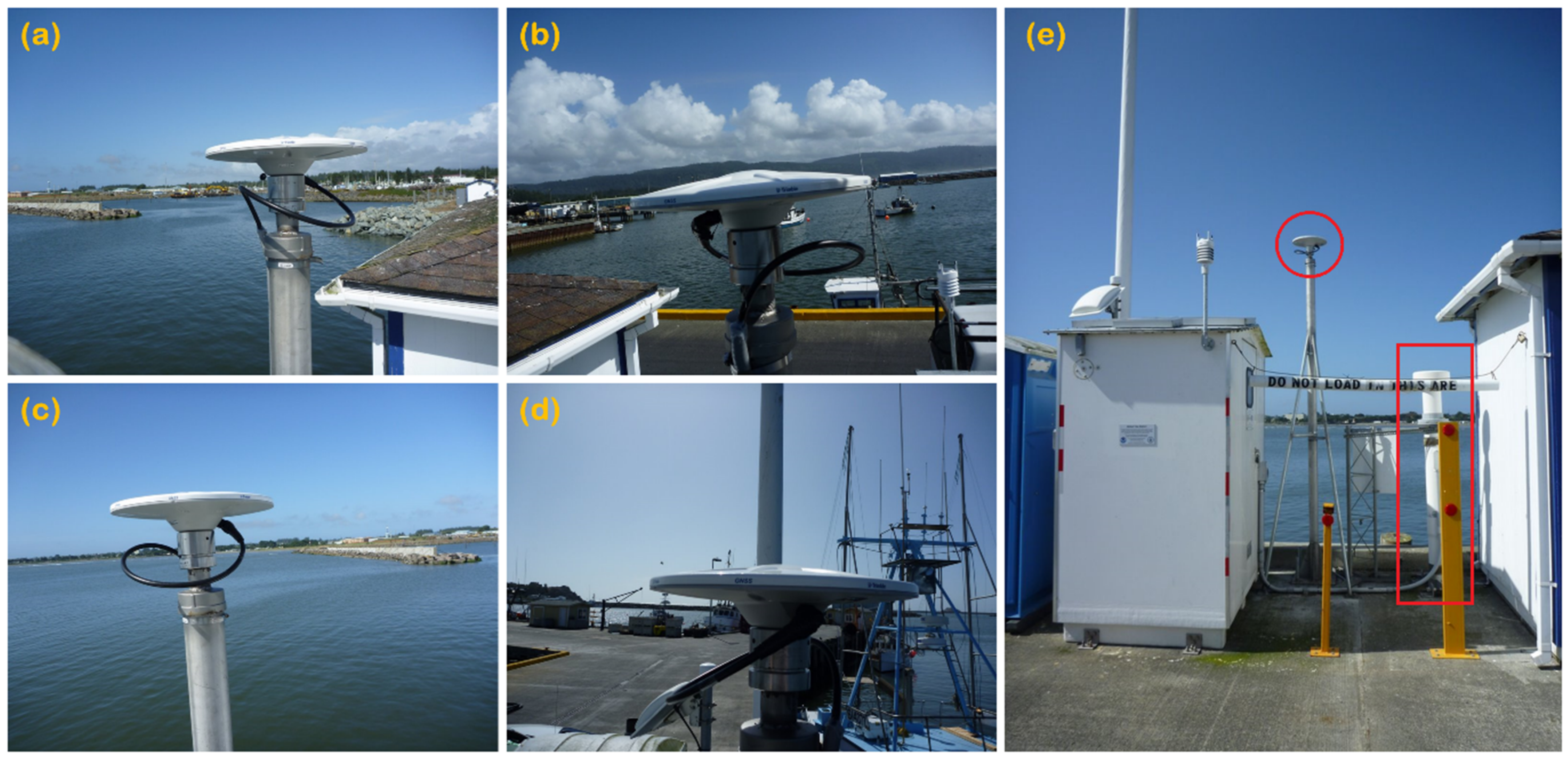
Figure 1.
The photographs show the surrounding area of CACC in Crescent City, CA (taken from NGS’s CACC website): (a) north view, (b) east view, (c) west view, (d) south view, and (e) antenna of CACC CORS marked as red circle and co-located NOAA tide gauge marked as red box (NOAA station ID: 9419750).

Figure 2.
First Fresnel Zone (FFZ) at CACC in Crescent City, CA, computed by GNSS-IR software package (https://www.ngs.noaa.gov/gps-toolbox/GNSS-IR.htm, accessed on 1 March 2021) using elevation angle in the range of 5° to 45° and azimuth angle in the range of −125° to +30°. The antenna height from the water surface of 6 m was applied.

Figure 3.
Time series of water levels derived by GNSS-R based tide gauge (red dots) together with water levels from the co-located tide gauge (blue dots) during the 2012 Canada tsunami. The magnification plots in upper left (a) and lower right (b) are the time series during normal condition and the tsunami event, respectively.

Figure 4.
Correlation coefficient between water level measurements from GNSS-R based tide gauge and the conventional tide gauge during the 2012 Canada tsunami. Center line (x = y) is shown as solid black line and the correlation coefficient is indicated in bottom right of the plot.
Figure 4.
Correlation coefficient between water level measurements from GNSS-R based tide gauge and the conventional tide gauge during the 2012 Canada tsunami. Center line (x = y) is shown as solid black line and the correlation coefficient is indicated in bottom right of the plot.

Figure 5.
The examples of the spectral domain during (a) calm and (b) rough conditions: all peaks detected in the spectral domain are marked with X marks, and the dominant peaks are marked with circles.
Figure 5.
The examples of the spectral domain during (a) calm and (b) rough conditions: all peaks detected in the spectral domain are marked with X marks, and the dominant peaks are marked with circles.

Figure 6.
The impact of the 2012 Canada tsunami in Crescent city, CA: (a) Time series of the CLR; (b) tsunami waves extracted through high-pass filter. The red solid line indicates the tsunami arrival time published by NOAA and the red box indicates the tsunami period (Oct 28 05:44–Oct 29 12:00) detected from tide gauge.

Figure 7.
Time series of water levels derived by GNSS-R based tide gauge (red dots) together with water levels from the co-located tide gauge (blue dots) during the 2015 Chile tsunami. The magnification plots in (a) upper left and (b) lower right are the time series during normal condition and the tsunami event, respectively.

Figure 8.
Correlation coefficient between water level measurements from GNSS-R based tide gauge and the conventional tide gauge during the 2015 Chile tsunami. Center line (x = y) is shown as solid black line and the correlation coefficient is indicated in bottom right of the plot.
Figure 8.
Correlation coefficient between water level measurements from GNSS-R based tide gauge and the conventional tide gauge during the 2015 Chile tsunami. Center line (x = y) is shown as solid black line and the correlation coefficient is indicated in bottom right of the plot.

Figure 9.
The impact of the 2015 Chile tsunami in Crescent City, CA: (a) Time series of the CLR; (b) tsunami waves extracted through high-pass filter (bottom). The red solid line indicates the tsunami arrival time published by NOAA, and the red box indicates the tsunami period (September 17–20) detected from tide gauge. The secondary tsunami component detected from the tide gauge is shown as a blue box.

Figure 10.
First Fresnel Zone (FFZ) at CALC in Cameron, LA, computed by GNSS-IR software package (https://www.ngs.noaa.gov/gps-toolbox/GNSS-IR.htm, accessed on 1 March 2021) using elevation angle in the range of 10° to 90° and azimuth angle in the range of 0° to 360°. The antenna height from the water surface of 12 m was applied. The photo on the bottom right shows the surrounding area of the NWLON sentinel station (station ID: 8768094).

Figure 11.
Time series of water levels derived by GNSS-R based tide gauge (red dots) together with water levels from the co-located tide gauge (blue dots) in Cameron, LA.
Figure 11.
Time series of water levels derived by GNSS-R based tide gauge (red dots) together with water levels from the co-located tide gauge (blue dots) in Cameron, LA.

Figure 12.
Correlation coefficient between water level measurements from GNSS-R based tide gauge and the conventional tide gauge during (a) the entire processing period and (b) the period of Harvey. Center line (x = y) is shown as a solid black line, and the correlation coefficients are indicated in bottom right of the plots.

Figure 13.
The impact of the 2017 Harvey in Cameron, LA: (a) Time series of the CLR; (b) storm surge components extracted through high-pass filter. The red box indicates the period of Harvey (Aug 24 12:00–Aug 30 24:00) detected from tide gauge.
Figure 13.
The impact of the 2017 Harvey in Cameron, LA: (a) Time series of the CLR; (b) storm surge components extracted through high-pass filter. The red box indicates the period of Harvey (Aug 24 12:00–Aug 30 24:00) detected from tide gauge.

Figure 14.
Map showing the location of AT01 PBO station in St. Michael and NOAA tide gauge station (ID: 9468333) in Unalakleet. The red box on the map represents the area of the enlarged map at the bottom right of the map. The FFZ computed by GNSS-IR software package using the given elevation and azimuth angle are shown in the enlarged map.

Figure 15.
Time series of water levels derived by GNSS-R based tide gauge (red dots) together with water levels from the co-located tide gauge (blue dots) in St. Michael, AK. The period of the storm surge is indicated as the red box.
Figure 15.
Time series of water levels derived by GNSS-R based tide gauge (red dots) together with water levels from the co-located tide gauge (blue dots) in St. Michael, AK. The period of the storm surge is indicated as the red box.

Figure 16.
Correlation coefficient between water level measurements from GNSS-R based tide gauge and the conventional tide gauge during the entire processing period (blue dots) and the period of the storm surge (green dots). Center line (x = y) is shown as solid black line, and the correlation coefficients are indicated in bottom right of the plot.

Figure 17.
The impact of the storm surge in St. Michael, AK: Time series of the CLR (blue) and the sea level measurements from the GNSS-R based tide gauge (orange). The red box indicates the period of the storm surge (Feb 12 00:00–Feb 13 12:00).
Figure 17.
The impact of the storm surge in St. Michael, AK: Time series of the CLR (blue) and the sea level measurements from the GNSS-R based tide gauge (orange). The red box indicates the period of the storm surge (Feb 12 00:00–Feb 13 12:00).


Table 1.
Statistical analysis of the water level differences between GNSS-R based tide gauge and the co-located tide gauge during the 2012 Canada tsunami.
Table 1.
Statistical analysis of the water level differences between GNSS-R based tide gauge and the co-located tide gauge during the 2012 Canada tsunami.
| Entire Processing Period (15 Oct–13 Nov) | Period of the Tsunami Event (28 Oct 05:44*–29 Oct 12:00) | |
|---|---|---|
| Mean [m] | 0.189 | 0.217 |
| RMS [m] | 0.230 | 0.257 |
| Median [m] | 0.170 | 0.209 |
| Std. [m] | 0.132 | 0.138 |
* 28 Oct 05:44: Tsunami arrival time at the tide gauge in Crescent city published by NOAA.
Table 2.
Statistical analysis of the water level differences between GNSS-R based tide gauge and the co-located tide gauge during the 2015 Chile tsunami.
Table 2.
Statistical analysis of the water level differences between GNSS-R based tide gauge and the co-located tide gauge during the 2015 Chile tsunami.
| Entire Processing Period (1 Sep –30 Sep) | Period of the Tsunami Event (17 Sep 13:39*–20 Sep 3:00) | |
|---|---|---|
| Mean [m] | 0.201 | 0.144 |
| RMS [m] | 0.243 | 0.190 |
| Median [m] | 0.181 | 0.109 |
| Std. [m] | 0.137 | 0.124 |
* 17 Sep 13:39: Tsunami arrival time at the tide gauge in Crescent city published by NOAA.
Table 3.
Statistical analysis of the water level differences between GNSS-R based tide gauge and the co-located tide gauge in Cameron, LA.
Table 3.
Statistical analysis of the water level differences between GNSS-R based tide gauge and the co-located tide gauge in Cameron, LA.
| Entire Processing Period (14 Aug –7 Sep) | Period of Harvey (24 Aug 12:00–30 Aug 24:00) | |
|---|---|---|
| Mean [m] | 0.027 | 0.037 |
| RMS [m] | 0.038 | 0.055 |
| Median [m] | 0.020 | 0.028 |
| Std. [m] | 0.027 | 0.041 |
Table 4.
Statistical analysis of the water level differences between GNSS-R based tide gauge in St. Michael and the tide gauge in Unalakleet.
Table 4.
Statistical analysis of the water level differences between GNSS-R based tide gauge in St. Michael and the tide gauge in Unalakleet.
| Entire Processing Period (26 Jan–19 Feb) | Period of the Storm Surge (12 Feb 00:00–13 Feb 12:00) | |
|---|---|---|
| Mean [m] | 0.140 | 0.410 |
| RMS [m] | 0.200 | 0.540 |
| Median [m] | 0.104 | 0.309 |
| Std. [m] | 0.142 | 0.352 |
Publisher’s Note: MDPI stays neutral with regard to jurisdictional claims in published maps and institutional affiliations. |
© 2021 by the authors. Licensee MDPI, Basel, Switzerland. This article is an open access article distributed under the terms and conditions of the Creative Commons Attribution (CC BY) license (http://creativecommons.org/licenses/by/4.0/).
Share and Cite
MDPI and ACS Style
Kim, S.-K.; Lee, E.; Park, J.; Shin, S. Feasibility Analysis of GNSS-Reflectometry for Monitoring Coastal Hazards. Remote Sens. 2021, 13, 976. https://0-doi-org.brum.beds.ac.uk/10.3390/rs13050976
AMA Style
Kim S-K, Lee E, Park J, Shin S. Feasibility Analysis of GNSS-Reflectometry for Monitoring Coastal Hazards. Remote Sensing. 2021; 13(5):976. https://0-doi-org.brum.beds.ac.uk/10.3390/rs13050976
Chicago/Turabian StyleKim, Su-Kyung, Eunju Lee, Jihye Park, and Sungwon Shin. 2021. "Feasibility Analysis of GNSS-Reflectometry for Monitoring Coastal Hazards" Remote Sensing 13, no. 5: 976. https://0-doi-org.brum.beds.ac.uk/10.3390/rs13050976
Note that from the first issue of 2016, this journal uses article numbers instead of page numbers. See further details here.