Article

A Fixed-Threshold Method for Estimating Fractional Vegetation Cover of Maize under Different Levels of Water Stress

1
College of Mechanical and Electronic Engineering, Northwest A&F University, Xianyang 712100, China
2
Water Management and Systems Research Unit, USDA-ARS, 2150 Centre Avenue, Bldg. D., Fort Collins, CO 80526, USA
3
Key Laboratory of Agricultural Internet of Things, Ministry of Agriculture, Xianyang 712100, China
4
Department of Civil and Environmental Engineering, Colorado State University, Fort Collins, CO 80523, USA
*
Author to whom correspondence should be addressed.
Submission received: 20 January 2021 / Revised: 2 March 2021 / Accepted: 2 March 2021 / Published: 7 March 2021
(This article belongs to the Special Issue Improve Irrigation Management with Remote Sensing Technology)

Abstract

:
Accurate estimation of fractional vegetation cover (FVC) from digital images taken by commercially available cameras is of great significance in order to monitor the vegetation growth status, especially when plants are under water stress. Two classic threshold-based methods, namely, the intersection method (T1 method) and the equal misclassification probability method (T2 method), have been widely applied to Red-Green-Blue (RGB) images. However, the high coverage and severe water stress of crops in the field make it difficult to extract FVC stably and accurately. To solve this problem, this paper proposes a fixed-threshold method based on the statistical analysis of thresholds obtained from the two classic threshold approaches. Firstly, a Gaussian mixture model (GMM), including the distributions of green vegetation and backgrounds, was fitted on four color features: excessive green index, H channel of the Hue-Saturation-Value (HSV) color space, a* channel of the CIE L*a*b* color space, and the brightness-enhanced a* channel (denoted as a*_I). Secondly, thresholds were calculated by applying the T1 and T2 methods to the GMM of each color feature. Thirdly, based on the statistical analysis of the thresholds with better performance between T1 and T2, the fixed-threshold method was proposed. Finally, the fixed-threshold method was applied to the optimal color feature a*_I to estimate FVC, and was compared with the two classic approaches. Results showed that, for some images with high reference FVC, FVC was seriously underestimated by 0.128 and 0.141 when using the T1 and T2 methods, respectively, but this problem was eliminated by the proposed fixed-threshold method. Compared with the T1 and T2 methods, for images taken in plots under severe water stress, the mean absolute error of FVC obtained by the fixed-threshold method was decreased by 0.043 and 0.193, respectively. Overall, the FVC estimation using the proposed fixed-threshold method has the advantages of robustness, accuracy, and high efficiency, with a coefficient of determination (R2) of 0.99 and root mean squared error (RMSE) of 0.02.

1. Introduction

Under climate change, water stress has become a great challenge to maize products globally. In research on crop yield, non-destructive monitoring of crop structural traits is of great significance. As one of the most widely used structural traits, fractional vegetation cover (FVC), defined as the proportion of ground surface occupied by green vegetation [1], plays an important role in monitoring vegetation growth status and estimating crop yields (e.g., evapotranspiration and above-ground biomass) [2,3,4]. In addition, FVC is also a key parameter in the AquaCrop model, which is widely used to simulate crop yield response to water under different irrigation and field management practices [5,6]. Therefore, it is important to estimate FVC rapidly and accurately for annual crops under different irrigation treatments during crop growing seasons.
Visual estimation, direct sampling, and digital photography have been developed to measure FVC for agricultural applications [7,8]. With the development of sensor technology, many researchers have used Red-Green-Blue (RGB) digital cameras [9,10,11] or near infrared (NIR) spectral sensors [12] in the field of agriculture. However, RGB digital imagery has been used more widely than NIR spectral sensors in image segmentation, with the advantages of low cost and higher spatial resolution. With the availability of inexpensive high-quality digital cameras in agriculture applications, estimating FVC by image segmentation is becoming more common. In general, image-based FVC estimation can be grouped into two categories: (1) machine learning methods (e.g., K-means, Decision Tree, Artificial Neural Networks, and Random Forest) [13,14,15] and (2) threshold-based methods [16,17]. Machine learning methods need a large amount of training data sets for the purposes of calibration. The generation of training data, affected by human intervention, has a great influence on model accuracy. Threshold-based methods, with their advantages of simplicity, high efficiency, and accuracy, play an important role in precision agriculture [18], and have been successfully used for crops such as wheat, maize, cotton, and sugar beet [12,19,20,21].
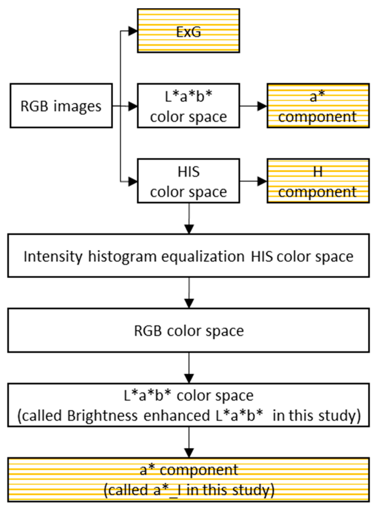
Selecting an appropriate color feature for crop segmentation is a key step to obtain FVC estimations using threshold-based methods [17,22]. Excessive green index (ExG) [23,24], H channel of the Hue-Saturation-Value (HSV) color space [25], and a* channel of the CIE L*a*b* color space [26] are the three widely used color features. The visible spectral index, ExG, can be calculated directly from digital numbers in three components of RGB images, and represents the contrast of the green spectrum against red and blue [24]. The H channel from the HSV color space uses an angle from 0° to 360° to represent different colors [27]. The a* channel from the CIE L*a*b* color space is relative to the green-red opponent colors [26]. In addition, to deal with the shadow effect in classification, the Shadow-Resistant LABFVC (SHAR-LABFVC) method was proposed [28]. In the SHAR-LABFVC method, the CIE L*a*b* color space, from which the a* color feature was extracted, was transformed from the brightness-enhanced RGB. To distinguish it from the a* color space in other research [26], the a* color feature in the SHAR-LABFVC method is denoted as the a*_I color feature in this study.
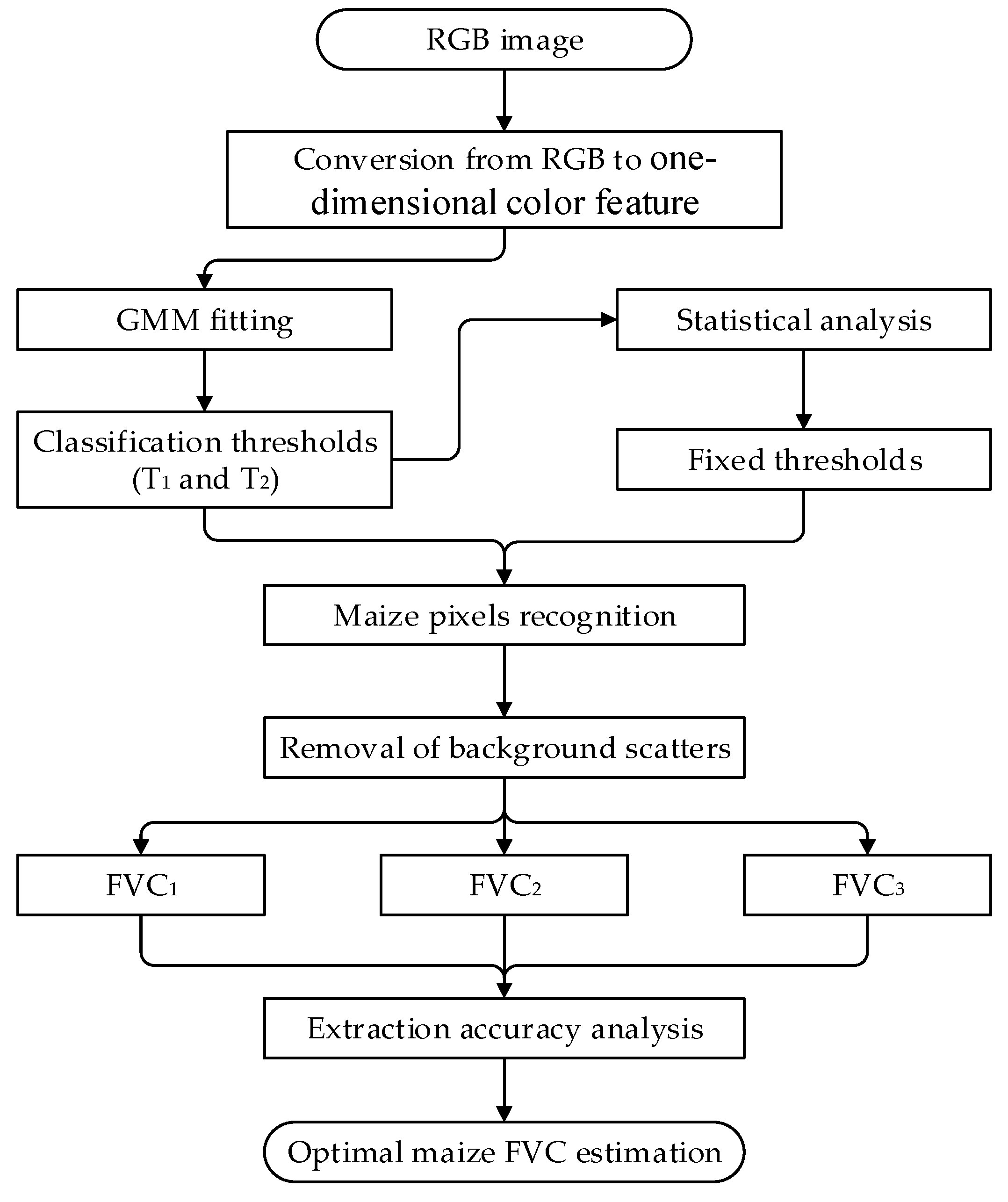
Another key step to obtain FVC estimations using threshold-based methods is searching for the appropriate classification threshold. Otsu’s method is one of the most widely used threshold techniques [29], and has been used in many applications of image segmentation and plant detection [30,31,32]. However, this method can produce under-segmentation in some circumstances [
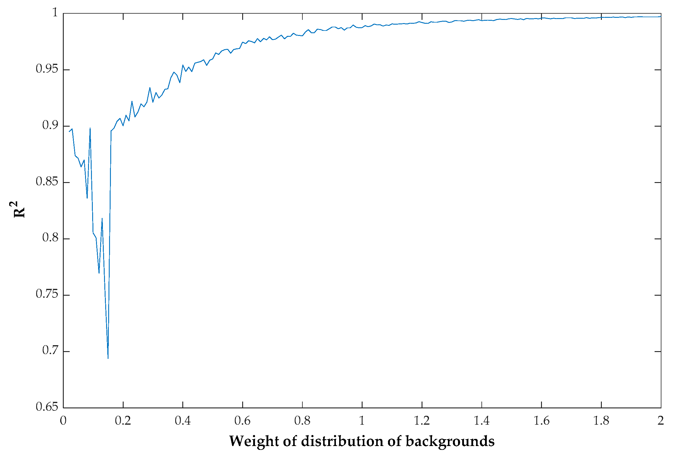
18]. Another widely used threshold method was proposed by [16] based on a Gaussian mixture model (GMM) of color features derived from images. Specifically, a Gaussian mixture model is a parametric probability density function represented as a weighted sum of Gaussian component densities. Classification thresholds for discriminating vegetation and backgrounds can be calculated from a GMM fitted on different color features. Fitting a GMM on an appropriate color feature contributes to accurate threshold calculation.
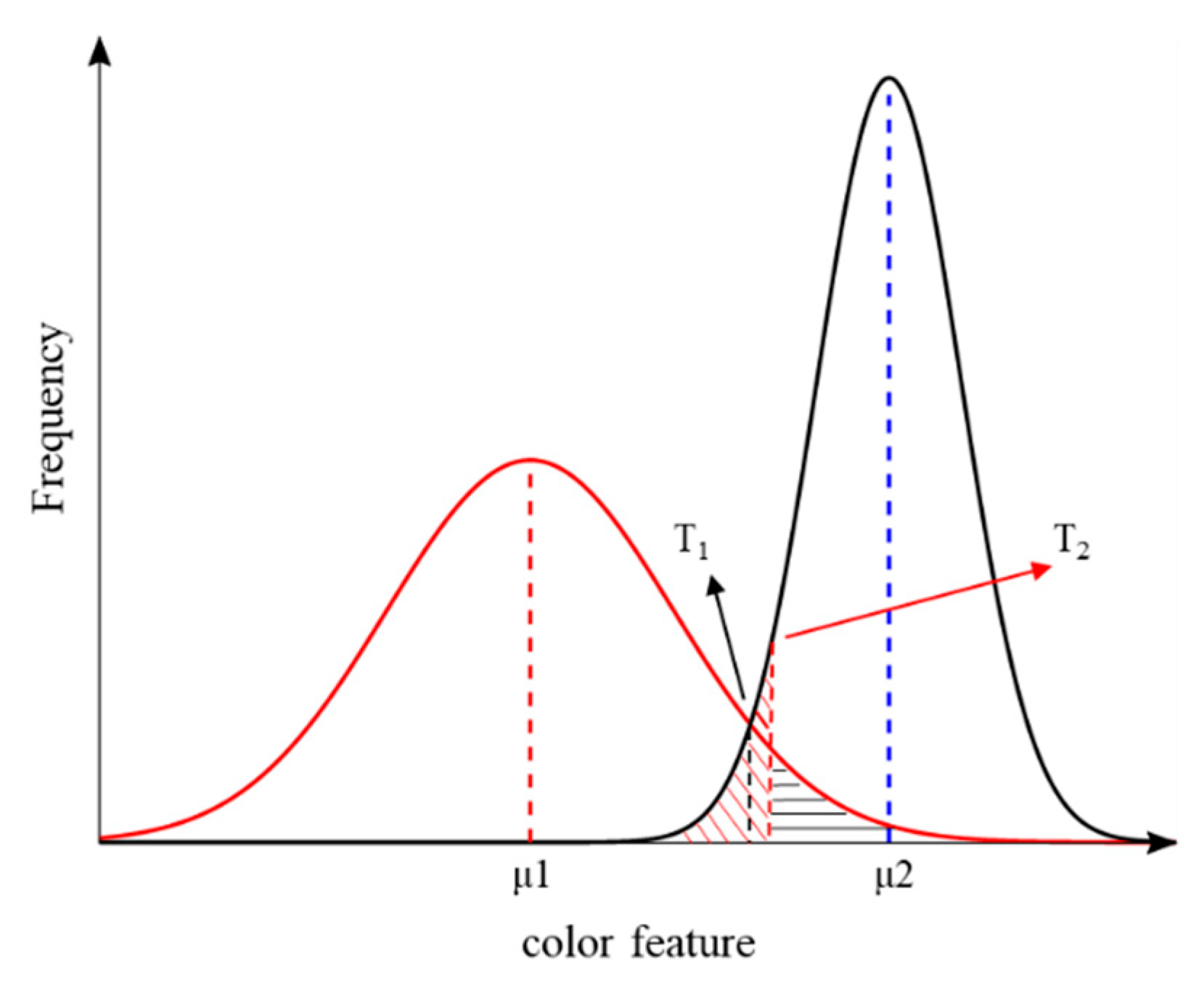
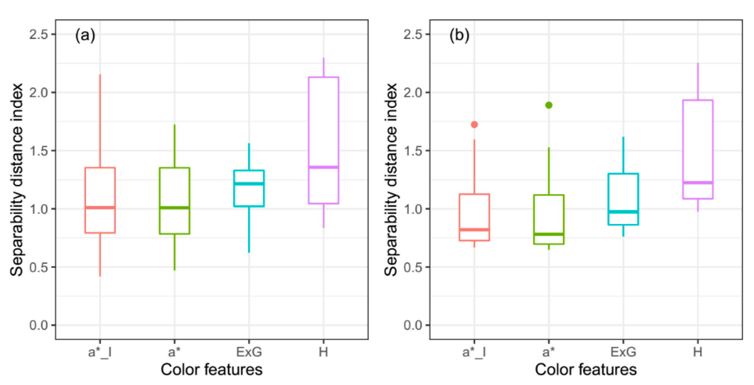
To evaluate the separability of two Gaussian distributions on different color features, the separability distance index (SDI) [26] and the instability index (ISI), which is the reciprocal of SDI [33], were proposed. SDI (Equation (1)) describes the separability of the distributions between vegetation and backgrounds,
SDI = | μ v μ b | σ v + σ b
where μ v and μ b are mean values of green vegetation and backgrounds, respectively; and σ v and σ v are standard deviations of green vegetation and backgrounds, respectively. The larger the SDI is, the easier it is to fit these two Gaussian distributions. However, whether the SDI is an appropriate criterion for selecting the right color feature to produce the best performance of GMM fitting is still uncertain and has not been explored in previous research. It is necessary to further study the applicability of SDI in selecting color features.
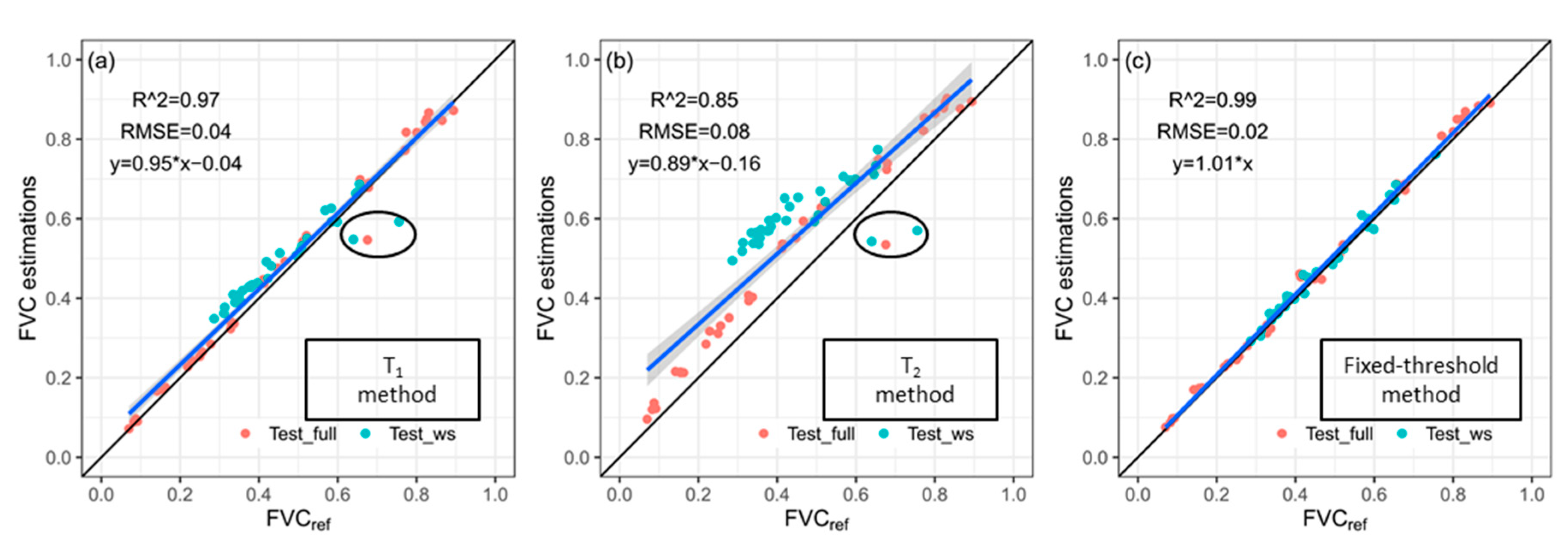
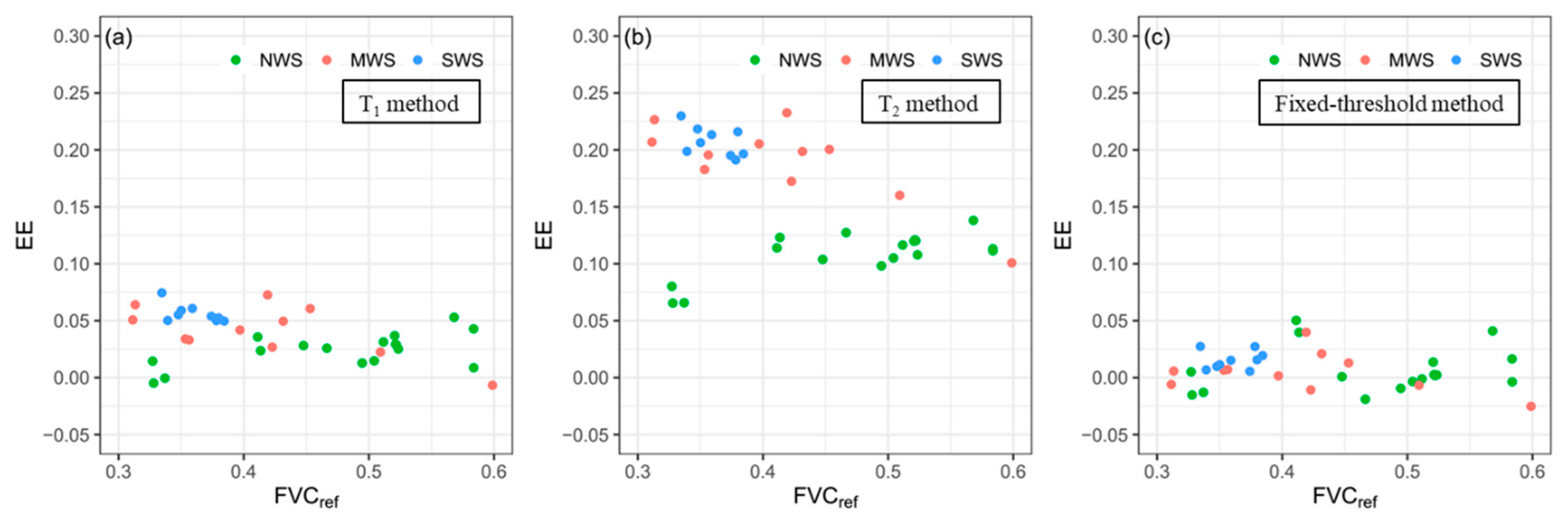
With GMM fitted on an appropriate color feature, applying an optimal approach to obtain the classification threshold is essential for calculating FVC. Once the parameters for both Gaussian distributions of vegetation and backgrounds have been estimated, classification thresholds can be calculated by two classic methods, namely, the intersection method, and the equal misclassification probability method. In the intersection method, the intersection of the two Gaussian distributions is used as the classification threshold (hereinafter referred to as T1). In the equal misclassification probability method (hereinafter referred to as T2), the threshold makes the green vegetation and backgrounds have an equal misclassification probability [26]. Both two classic methods derive thresholds based on the Gaussian distributions of green vegetation and backgrounds in each image.
However, both the two abovementioned threshold methods have limitations. Firstly, both perform well when the bimodality is clearly seen in the distributions of images on a color feature; however, when FVC is extremely low or the canopy is nearly closed, the thresholds obtained by these methods may be inaccurate. Secondly, in semi-arid and arid areas, where climate is characterized by long periods of drought with decreasing projected rainfall, the high possibility of crops suffering from water stress may raise a new challenge for FVC estimation caused by spectral changes. To cope with water stress, crops usually exhibit adaptive mechanisms at the leaf level to reduce light absorption and dissipate excess absorbed energy, such as the decrease in chlorophyll concentration and down-regulation of photosynthesis, and increase in the concentration of deep oxidized xanthophyll cycle components [34,35,36,
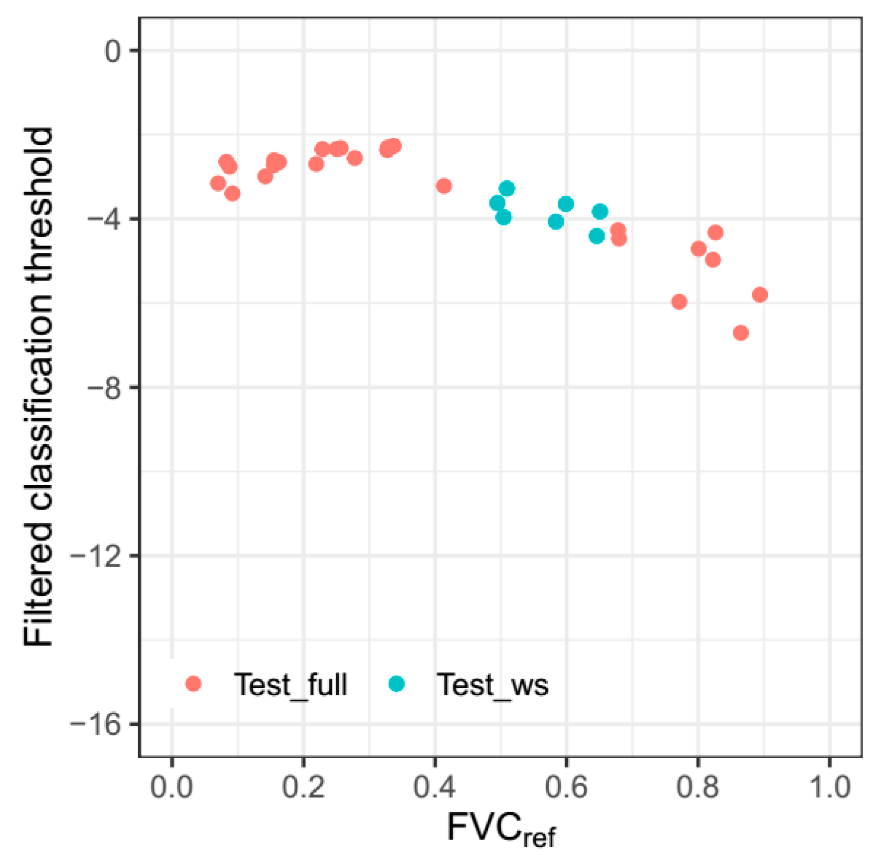
37]. The spectral changes of crops caused by the pigment changes at the leaf level may have a great influence on the accuracy of threshold calculation using the two methods. Therefore, RGB images collected across the entire crop growing season with a wider FVC range and different levels of water stress conditions need to be further studied regarding the performance of FVC estimation using threshold methods based on GMM. In addition, in our previous research for cotton FVC estimation [21], an interesting phenomenon was found: a fixed classification threshold exists in the a* channel. Therefore, further study is needed to determine if there is a fixed classification threshold for maize.
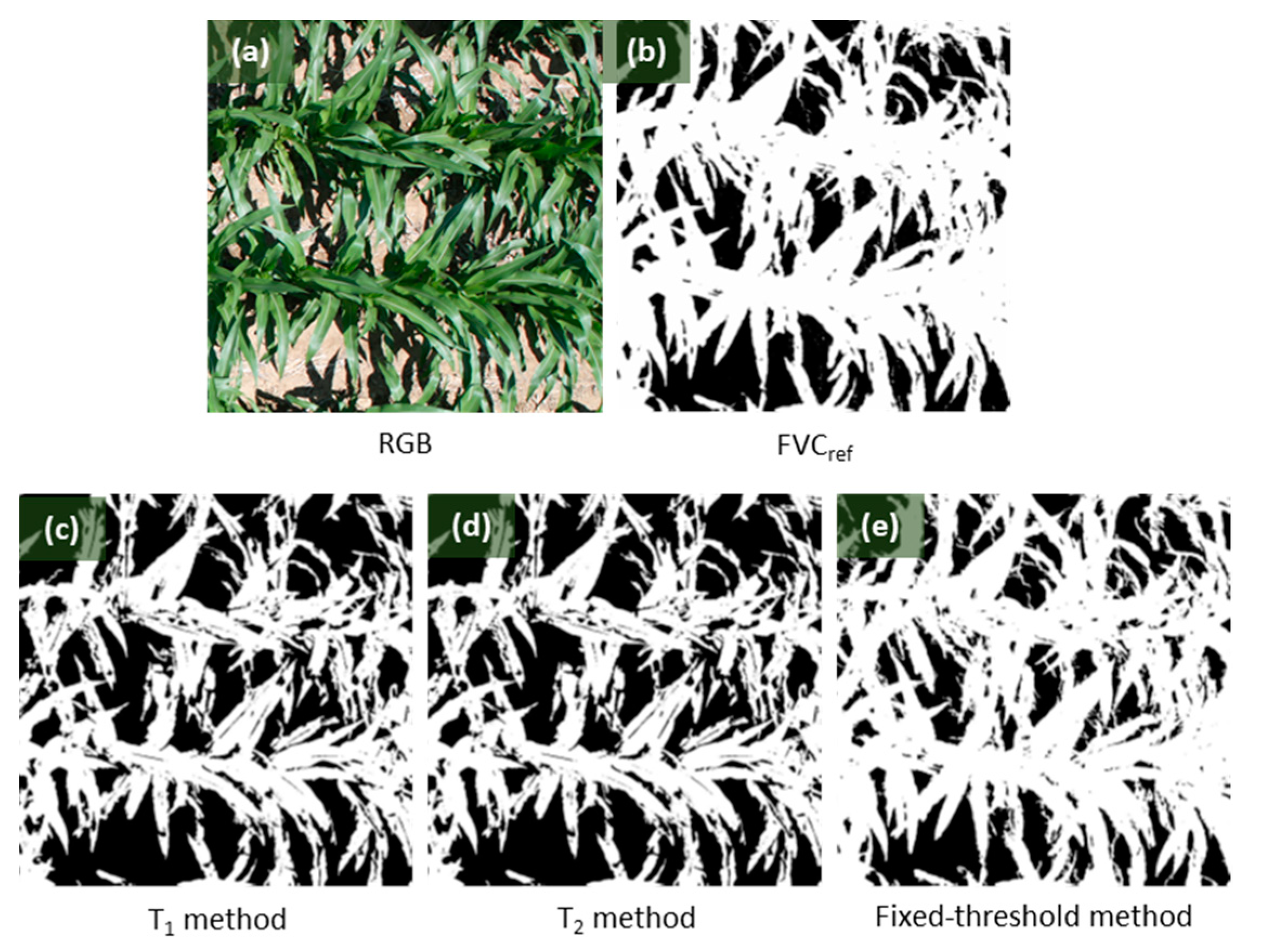
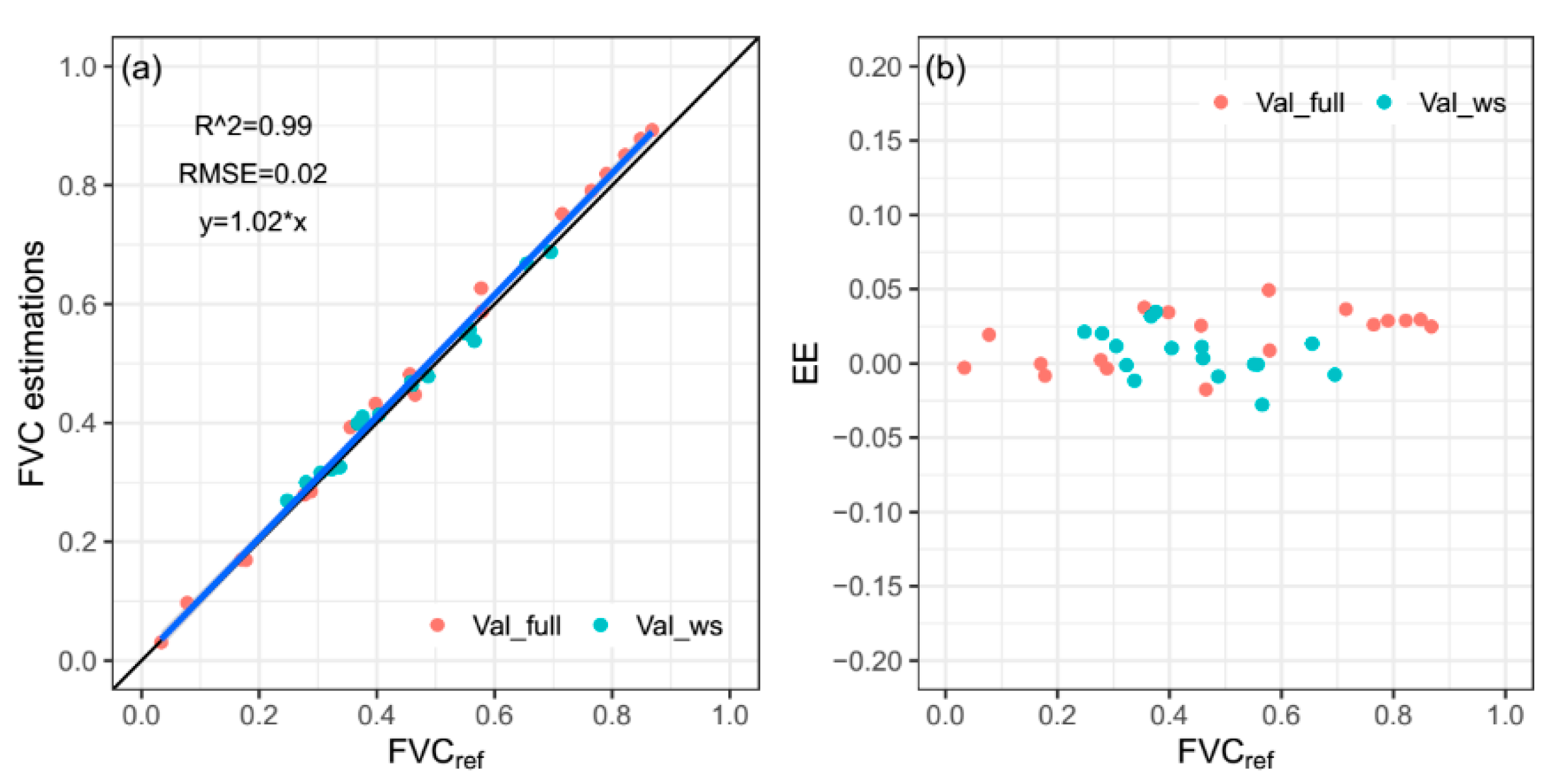
In this study, there were two main objectives: (1) to determine if a fixed-threshold method exists and is applicable for images covering the full range of FVC from open to nearly closed; (2) to explore if the fixed-threshold method outperforms the two classic threshold-based methods (T1 and T2 methods) in estimating FVC for images with high reference FVC or captured from deficit irrigation plots. This research could provide a more practical, efficient, and accurate way to estimate the FVC of field maize under water stress based on RGB imagery.

2. Materials

2.1. Study Site and Management

Field experiments were conducted during 2013, 2015, and 2016 growing seasons at the USDA-ARS Limited Irrigation Research Farm, in Greeley, Colorado, USA (40°26′57″N, 104°38′12″W, elevation 1427 m). The maize (Zea mays L.) was planted with 0.76 m row spacing on May 14 (day of year, DOY 134), June 3 (DOY 154), and May 5 (DOY 126) in 2013, 2015, and 2016, respectively. Twelve irrigation treatments (TRTs) (Table 1), each 9 m wide by 43 m long, were randomly arranged with four replications (Figure 1a). Deficit irrigation was applied during the late vegetative and maturation growth stages. The dates when maize reached the late vegetative stage (V8), beginning of reproductive stage (R1), and beginning of maturation stage (R4) were July 1 (DOY 182), July 29 (DOY 210), and August 19 (DOY 231) for the 2013 growing season, respectively. In 2015, these dates were July 6 (DOY 187), August 3 (DOY 215), and August 24 (DOY 236), respectively. In 2016, these dates were June 27 (DOY 179), July 25 (DOY 207), and August 9 (DOY 222), respectively. Each treatment targeted a percent of maximum non-stressed crop evapotranspiration (ET) during late vegetative and maturation growth stages, respectively. Table 1 shows the sum of actual net irrigation amounts and precipitation for each treatment. Details can be found in [38] for the calculation of maximum ET.

2.2. Canopy Temperature and Meteorological Data Measurements

Infrared thermometers (IRT, model: SI-121, Apogee Instruments, Inc., Logan, UT, USA) were used to continuously monitor maize canopy temperature. The view angle and accuracy were 36° and ±0.2 °C, with a temperature range of −10 °C to 65 °C. To ensure the maize canopy was primarily included in the field of view, the IRTs were attached to telescoping posts and angled 23° below horizon and 45° from north (looking northeast). The IRTs were kept at a height of 0.8 m above the top of canopy with the viewing area of 13.35 m2 and adjusted twice per week during the vegetative stage. In 2013, IRT sensors were installed in six of the twelve treatments: TRT1 (100/100), TRT2 (100/50), TRT3 (80/80), TRT6 (80/40), TRT8 (65/65), and TRT12 (40/40). In 2015 and 2016, IRT sensors were installed for all treatments except for: TRT4 (80/65) and TRT6 (80/40).
Meteorological data were taken by the on-site Colorado Agricultural Meteorological Network station GLY04 (CoAgMet), including daily precipitation, air temperature, relative humidity (and subsequent vapor pressure deficit), solar radiation, and wind speed taken at 2 m above a grass reference surface. The canopy temperature and meteorological data were used to calculate the crop water stress index (CWSI), which is one of the most frequently adopted indicators of crop water stress [39].

2.3. Crop Water Stress Index (CWSI)

The empirical CWSI method defined by [40] was adopted in this study. It is calculated as in Equation (2):
CWSI = dT m dT LL dT UL dT LL
where dTm is the difference between measured canopy and air temperature; dTLL and dTUL are the lower and upper limits of canopy-air temperature differential. CWSI values of 0 indicate no stress and values of 1 indicate maximum stress. In this study, 5 °C was used as the upper baseline. The actual CWSI could be slightly greater than 1, due to the fact that measured dTm values could be occasionally greater than the upper baseline [41]. The lower baseline for 2013, 2015, and 2016 can be found in Equations (3)–(5), respectively:
dT LL = 1.79 × VPD + 2.34
dT LL = 1.97 × VPD + 3.43
dT LL = 2.76 × VPD + 4.98
where VPD is the vapor pressure deficit of the atmosphere with the unit of kPa. VPD is related to air temperature and relative humidity, and can be calculated by Equation (6) [42]:
VPD = 0.6108 × exp ( 17.27 T a T a + 237.3 ) × ( 100 RH 100 )
where Ta is air temperature with the unit of °C, and RH is relative humidity.

2.4. RGB Image Acquisition

A Canon EOS 50D DSLR camera (Canon Inc., Tokyo, Japan) was attached to a boom that was mounted on a high clearance tractor and then elevated about 7 m above the ground. The sensor size and resolution were 22.3 mm × 14.9 mm and 4752 × 3168 pixels. The target view of the ground was about 5.7 m × 3.8 m at the center row of each plot (encompassing 5 rows, Figure 1b), and due to the adoption of the small resolution mode (2352 pixels × 1568 pixels), the pixel size of images was about 0.24 cm. Nadir view RGB images were taken near solar noon from each treatment plot. Figure 1a shows the capturing route of RGB images. Detailed RGB image collection dates are shown in Table 2.

2.5. Image Selection

To better evaluate the adaptability of the proposed method in this study to different FVC levels and water stress levels, a total of 102 RGB images were selected from 2013, 2015, and 2016 growing seasons. These images cover the full range of FVC from open to nearly closed. Of these images, 54 were taken from fully irrigated plots (TRT1) to test the adaptability of the new method to different FVC levels, and 48 were taken from plots under different irrigation treatments to test the adaptability of the new method to different water stress levels. Specifically, water stress levels were defined using CWSI: no water stress (NWS) when CWSI was less than 0.20; intermediate water stress (MWS) when CWSI was between 0.20 and 0.60; and severe water stress (SWS) when CWSI was greater than 0.60. The 54 images taken from TRT1 were divided into the test image group (hereinafter referred to as Test_full) and the validation image group (hereinafter referred to as Val_full) with a ratio of 2:1. In the same way, the 48 images with different levels of water stress were divided into Test_ws and Val_ws groups. Deficit irrigation started from the late vegetative stage when FVCref reached about 0.50 for maize from fully irrigated plots, and images from Test_ws and Val_ws sets were captured after the late vegetative stage. Therefore, compared with the Test_full and Val_full image sets, the lower limits of FVCref of Test_ws and Val_ws image sets were higher. The details of all these 102 images are listed in Table 3.

3. Methodology

Three main steps were taken to estimate maize FVC based on RGB images: (1) extraction of four color features, namely, a*_I, a*, ExG, and H; (2) classification threshold computation and analysis; and (3) removal of background scatters based on the morphological differences between maize plant and background scatters. Details can be found hereafter for these three steps. Figure 2 shows the procedure of maize FVC estimation using three different threshold-based methods. In this study, proximally sensed RGB images were processed and analyzed by using custom-written scripts programmed in R language (R-3.5.3, https://www.r-project.org/ (accessed on 1 June 2020)).

3.1. Aquisition of Four Color Features

The selection of an appropriate color feature contributes to a better performance in image segmentation. In this study, four color features, a*_I, a*, ExG, and H, were extracted from CIE L*a*b*, RGB, and HIS color spaces. The calculation process is shown in Figure 3, and the four color features are highlighted using rectangles covered with orange lines.

3.2. Approaches to Calculating the Thresholds for Image Segmentation

In proximally sensed images, the distributions of vegetation and backgrounds were assumed to follow GMM on one color feature. With the assumption of only two classes in these images [20], the GMM function can be given by:
F ( x ) = ω v × N ( μ v , σ v 2 ) + ω b × N ( μ b , σ b 2 )
where ω , μ , σ and are weight, mean value, and standard deviation, respectively; subscript v and b represent vegetation and backgrounds, respectively; N ( μ , σ 2 ) represents the Gaussian distribution function; and x is the value of image on the color feature. The GMM function was fitted using the “mixtools” package in R [43].
Two classic threshold methods: the two Gaussian distribution curves of GMM shown in Figure 4 represent the distributions of green vegetation and backgrounds, respectively. Based on the GMM fitted on one color feature, T1 can be calculated by solving Equation (8).
ω v × N ( μ v , σ v 2 ) = ω b × N ( μ b , σ b 2 )
Secondly, the threshold obtained using the T2 method made the misclassification probabilities of green vegetation and backgrounds equal. As shown in Figure 4, T2 can be calculated by solving a complementary error function as in Equation (9):
ω v × e r f c ( μ v , σ v 2 ) = ω b × e r f c ( μ b , σ b 2 )
where e r f c is the complementary Gaussian error function. Classification thresholds and FVC estimation were obtained using these two approaches. To distinguish different combinations of two threshold calculation methods and four color features, they are denoted using the color feature name and threshold calculation name with an underscore between them. For example, a*_I_T1 is used to represent the combination of the T1 method and the a*_I color feature.
The fixed-threshold method was proposed based on the statistical analysis of one of the classic methods which performs better in FVC estimation. If a real threshold which generates the reference FVC (FVCref) of maize exists, the smaller the absolute estimation error, the closer the thresholds calculated from the T1/T2 method are to the real threshold. In this study, we set the upper limit of absolute estimation error at 0.025 to get a more accurate threshold. Therefore, in the statistical analysis, only the thresholds which made the absolute estimation error of FVC less than 0.025 were used. The thresholds calculated from RGB images with FVCref less than 0.5 were averaged. Then, the average value was referred to as the initial threshold of the fixed-threshold method. On the other hand, the average of thresholds obtained from the images with FVCref greater than 0.5 was used as the adjusted threshold of the fixed-threshold method.

3.3. Removal of Scatters and Spurs Using Morphological Method

Considering that the GMM model is fitted based on the distribution of color features of each pixel, there are two main drawbacks when estimating FVC using this method: it may generate misclassified scatters with a high probability, and the edge of the extracted vegetation may not be well preserved [22]. In this study, to remove misclassified scatters and to trim the edge of extracted vegetation, the morphological algorithm was adopted. After vegetation pixels were recognized, all extracted pixel clusters (including misclassified scatters) could be treated as regions with different numbers of pixels. In general, misclassified scatters were regions with small numbers of pixels. Therefore, the size of the pixel cluster area was used as the criterion to decide whether it was a misclassified scatter. The optimal threshold used to remove the scatters was determined by comparing the differences between the FVC estimations and FVCref. The smallest difference was obtained when the threshold of 500 was used. It is worth noting that similar differences were obtained around the optimal threshold of 500. Thus, in this study, if the area of the pixel cluster was less than 500 pixels, it was treated as a misclassified scatter and was removed. As for trimming the edge of extracted vegetation, maize leaves should be closed regions with smooth edges. However, after vegetation pixels were recognized, small spurs often appeared on the edge. If the area of the pixel cluster on the edge of extracted vegetation was less than 500 pixels, it was treated as a spur and was removed.

3.4. Assessment of FVC Extraction Accuracy

The FVCref of all test images was obtained by supervised classification via Environment for Visualizing Images (ENVI; Exelis, Inc., Boulder, CO, USA). Due to the high resolution of proximal RGB images, the FVCref values obtained from this method are reliable [18,44]. Specifically, to get the accurate FVCref, training samples of about 12,000 pixels including pure green vegetation and pure backgrounds were selected for each image using the tool of New Region of Interest in ENVI. Then, a supervised classification using support vector machine algorithm [45] was performed based on these training samples. Finally, a classified image was obtained, and the proportion of green vegetation was calculated as the FVCref. In addition, a set of test samples of about 8000 pixels was selected for each test image using the tool of New Region of Interest in ENVI, and was used to evaluate the accuracy of the classified image. For all classified images, the average of kappa coefficient was 0.983, and the average of overall accuracy was 99.1%. The results demonstrated that the FVCref values calculated from the classified images were accurate enough to assess the performance of FVC estimations of other methods. In this study, the performance of FVC estimations was assessed using the estimation error (EE) and mean absolute error (MAE), which were defined as:
EE = FVC FVC ref
MAE = 1 N i = 1 N EE i
where FVCref and FVC are reference FVC and FVC estimations derived from three threshold methods. N and i represent the total number of images and image index, respectively. In addition, the root mean squared error (RMSE) and the coefficient of determination (R2) were used to assess the correlation between FVCref and FVC obtained using different methods.

4. Results

4.1. Deficit Irrigation Results Evaluated by CWSI

The sensitivity of the CWSI empirical method for maize water stress has been verified within the same research field in previous studies [46,47]. Significant correlations were found between CWSI and classical water stress indicators (soil water deficit and sap flow). Figure 5 shows the seasonal trends of CWSI for TRT1(100/100), TRT3(80/80), TRT8(65/65), and TRT12(40/40). Clear differences among TRT1, 3, 8, and 12 were found for the 2015 growing season during the late vegetative stage when deficit irrigation was applied. The corresponding mean CWSI values for TRT1, 3, 8, and 12 were 0.06, 0.23, 0.69, and 0.90, respectively. With the release of deficit irrigation during the reproductive stage, all deficit irrigation treatments (TRT3, 8, and 12) had clear deceases, with mean CWSI values decreased to 0.02, 0.15, and 0.18, respectively. When deficit irrigation was re-imposed during the maturation stage, clear differences among TRT1, 3, 8, 11, and 12 showed again, with average CWSI values of 0.09, 0.26, 0.47, and 0.51. At the same time, it could be observed that the differences in CWSI became more obvious as deficit irrigation progressed, with values of 0.15, 0.32, 0.57, and 0.69 for TRT1, 3, 8, and 12 on DOY 253. Similar patterns were also observed for the 2013 and 2016 growing seasons. Overall, different levels of water stress were observed for all three maize growing seasons.

4.2. Comparison of Two Classic Methods on Four Color Features

The mean absolute error (MAE) of maize FVC estimations was calculated based on Test_full and Test_ws image sets (Table 4). Compared with the T2 method, the T1 method performed better with lower MAEs for all four color features. When the T1 method was used, the a*_I color feature performed best for both Test_full and Test_ws image sets with an MAE of 0.021 and 0.047, respectively. The H color feature resulted in the greatest MAE for Test_full (0.122) and Test_ws (0.150) among the four color features. The a* color feature generated greater MAEs than the ExG color feature for both Test_full and Test_ws image sets. All these results showed that the T1 method was better than the T2 method, and the a*_I color feature had the best robustness for images with the wide range of FVCref and with different water stress levels.

4.3. Calculation Results of Two Threholds in the Fixed-Threshold Method

Considering that a*_I_T1 outperformed all other methods used above, statistical analysis of thresholds was implemented based on the results of the a*_I_T1 method. The classification thresholds with absolute estimation error less than 0.025 obtained by the a*_I_T1 method are shown in Figure 6. For images with FVCref less than 0.5, the classification thresholds showed a small variation with a mean value of −2.72 and standard deviation of 0.39. Thus, the mean value of −2.72 was used as the initial threshold of the fixed-threshold method. On the other hand, there is a decreasing trend for classification thresholds when FVCref is greater than 0.5. To make the second fixed threshold applicable to most images with FVCref greater than 0.5, the average value of −4.60 was used as the adjusted threshold of the fixed-threshold method.

4.4. Results of FVC Estimations of Different Methods

4.4.1. Comparison based on Test Image Groups

Considering that a*_I outperformed all other color features, the following comparison was based on the a*_I color feature. The performance of FVC estimation using the T1 method, T2 method, and fixed-threshold method on the a*_I color feature is shown in Table 5. For both of the Test_full and Test_ws image groups, the fixed-threshold method performed best with smallest MAE and RMSE, and greatest R2, followed by the T1 method and then the T2 method. Compared with the T1 method, the MAE obtained by using the fixed-threshold method was decreased by 0.06 and 0.033 for Test_full and Test_ws, respectively. Compared with the T2 method, the MAE obtained by the fixed-threshold method was decreased by 0.058 and 0.154 for Test_full and Test_ws, respectively.
The correlation between FVCref and FVC estimations obtained by using three methods based on the test group images (Test_full and Test_ws) is shown in Figure 7. On one hand, for the images with high FVCref, captured from fully irrigated plots, the T1 and T2 methods performed unstably with some FVC estimations being underestimated, as shown in Figure 7a,b. However, it can be observed from Figure 7c that the fixed-threshold method worked well on all these images. Figure 8 shows the comparison of FVC maps obtained by applying three different methods to an image with high FVCref. It could be observed that the result of the fixed-threshold method was closer to the RGB image and the FVCref map.
On the other hand, for the images with different levels of water stress, the FVC results of T1 and T2 methods were overestimated as shown in Figure 7a,b, especially the FVC estimations by the T2 method. However, Figure 7c shows that the fixed-threshold method improved the FVC estimation accuracy of those images with different levels of water stress. In addition, for the T1 and T2 methods, the more severe the water stress, the more overestimated the FVC estimations. To provide a better explanation of this phenomenon, EEs of all test group images with FVCref ranging from 0.3 to 0.6 are shown in Figure 9. The limit condition of FVCref used to select an image can ensure that the effect only comes from different levels of water stress. As shown in Figure 9a,b, compared with the images taken in NWS and MWS plots, the EEs of images taken in SWS plots were higher when the T1 or T2 method was used. When the fixed-threshold method was used, the EEs of these images showed no big differences among the images regardless of water stress level, as shown in Figure 9c.

4.4.2. Validation of the Fixed-Threshold Method

To validate the performance of the fixed-threshold method, the initial threshold (−2.72) and the adjusted threshold (−4.60) were applied to the validation image groups (Val_full and Val_ws). The Val_full image group includes 18 images captured in fully irrigated plots. The Val_ws image group includes 16 images captured in plots suffering different levels of water stress. A high correlation (R2 = 0.99, RMSE = 0.02) between FVC estimations obtained by the fixed-threshold method and FVCref can be observed in Figure 10a. The EEs shown in Figure 10b were concentrated near 0, with a mean value of 0.012 and standard deviation of 0.018.

5. Discussion

5.1. Selecting the Appropriate Color Feature for a GMM-Based Threshold Method

The first key step to estimate crop FVC using a GMM-based threshold method is the selection of the appropriate color feature. In previous studies [25,26], the separability distance index (SDI) was proposed as the criterion to select the color feature. A larger SDI means that it should be easier to separate vegetation from non-vegetated backgrounds. However, in this study, the H channel had the largest SDI with mean values of 1.50 and 1.45 for Test_full and Test_ws image sets (Figure 11). At the same time, the greatest MAE was observed for the H channel among the four color features when the T1 method was used. The a*_I color feature outperformed other color features, with MAEs of 0.021 and 0.047 for Test_full and Test_ws image sets using the T1 method. These results indicate that the color feature with the largest SDI may not always result in a low FVC EE, and the SDI cannot be used as the sole criterion to choose an appropriate color feature. Once the Gaussian distributions of green vegetation and backgrounds can be successfully fitted within all the color features, the ability of each color feature to identify green vegetation may be the key to influence the FVC estimation accuracy [21]. Future studies are needed to quantify the ability of SDI to separate green vegetation from backgrounds within a color feature, and to find the threshold where the Gaussian distributions of vegetation and backgrounds can be accurately fitted.

5.2. The Fixed-Threshold Method Provides the Most Accurate FVC Estimations

Threshold-based approaches have been widely applied to RGB images with high spatial resolution. Some threshold methods are based on a GMM, which is fitted on one color feature derived from RGB images, representing the distribution of green vegetation and backgrounds [26]. However, these methods perform unstably when the canopy is nearly closed [9,48] and show an obvious overestimation when crops suffer from severe water stress. Firstly, to investigate the performance of GMM fitting of images with different levels of FVC, a sequence that fits the GMM was simulated and white noise was added to it. To make the sequence more practical, mean values and standard deviations similar to those from green vegetation and backgrounds on the a*_I color feature were used. Different levels of FVC were simulated by changing the weight of the distribution of backgrounds. All sequences representing different levels of FVC were processed to fit the GMM, and R2 was calculated based on the real GMM and the GMM fitted from the sequence. The change of R2 with the weight of the distribution of backgrounds is shown in Figure 12. The R2 was not stable and was less than 0.90 when the weight of the distribution of backgrounds is less than 0.2, which means that the GMM fitting and threshold results are not accurate when FVC is high.
Second, the FVC of crops under water stress was overestimated by these threshold methods based on GMM. More severe water stress led to higher MAE (Table 6). When the T1 method was used, the MAEs obtained from MWS and SWS plots were increased by 0.016 (61.5%) and 0.031 (119%), respectively, compared with those from NWS plots. A similar phenomenon was observed for the T2 method. This may result from the spectral changes of crops caused by pigment changes at the leaf level. Water stress can affect the leaf pigment content, such as chlorophyll content [36]. The leaf chlorophyll content decreases as crop water stress increases, resulting in a minimal reflectance in the green spectrum. The T1 and T2 methods were applied on the a*_I color feature, which is relative to the green-red opponent colors, with negative values toward green and positive values toward red. Therefore, green vegetation with lower chlorophyll content has a higher a*_I value, which makes it more difficult to distinguish green vegetation from the background. Further study is needed to explain this specifically.
In this study, the proposed fixed-threshold method addressed the problems mentioned above. Compared with the T1 and T2 methods, the new method exhibits stronger robustness, especially when the canopy is nearly closed (Table 5) and provides similar accuracy for images with different levels of water stress (Table 6). The new method is highly accurate and robust to different vegetation cover levels and water stress levels, with an overall RMSE of 0.02 and R2 of 0.99 for both test group images (Figure 7c) and validation group images (Figure 10a). Similar results were observed in [12], which showed that the optimal threshold of VARI images for sugar beet segmentation tends to be around a constant value of 0.14.
In the fixed-threshold method, the initial threshold was −2.72 for maize with FVCref less than 0.5, and the adjusted threshold was −4.60 for maize with FVCref equal to or greater than 0.5. The adjusted threshold is smaller than the initial threshold, which may be due to the changes in spectral reflectance at different FVC levels. In the visible spectrum, the reflectance of blue and red bands is negatively correlated with the FVC of maize [49]. However, there was no obvious correlation between the reflectance of the green band and the FVC of maize [49]. With the increase in maize FVC, the decrease in the reflectance of red and blue bands leads to a decrease in the a*_I color feature. Hence, for the maize with greater FVCref, the threshold is slightly lower than that of maize with smaller FVCref. The critical point was set at the FVC of 0.5 because there was an obvious change in threshold before and after 0.5 (Figure 6). The reason why the threshold changes a lot around an FVC 0.5 still needs to be studied in the future.
In addition to having higher FVC estimation accuracy and robustness, the proposed fixed-threshold method is simpler and more efficient. Once the initial threshold and the adjusted threshold have been obtained, the time to extract FVC of maize using the fixed-threshold method is less than the time using the T1 or T2 method. Taking the test group image as an example, the time to extract FVC using the fixed-threshold method is 43.63 and 56.05 s/per image faster than T1 and T2, respectively (Table 7).

6. Conclusions

This study proposed a fixed-threshold method based on the statistical analysis of the thresholds obtained using the T1 method. In this method, some images were selected and processed to obtain the initial threshold and the adjusted threshold, which can be applied to all images collected from plots with different levels of FVC and water stress. As such, the proposed method addressed the problems of robustness and accuracy that occur when the canopy is nearly closed, or when crops are subjected to water stress. Compared with the two threshold methods (T1 and T2 methods), the fixed-threshold method generated more accurate and robust FVC estimations, especially for maize with high FVC or under severe water stress. The performance of the fixed-threshold method was assessed based on FVCref with an RMSE of 0.02 and R2 of 0.99 for both test group images and validation group images. The results strongly suggest that the fixed-threshold method could provide an efficient and accurate way to obtain reference FVC used for validating FVC estimations obtained from UAV or satellite remote sensing platforms.

Author Contributions

Y.N. and L.Z. proposed the method and analyzed the data; Y.N., L.Z., H.Z. and H.C. discussed and drafted the manuscript. H.Z. and W.H. revised the manuscript and edited English language. All authors have read and agreed to the published version of the manuscript.

Funding

This research received no external funding.

Institutional Review Board Statement

Not applicable.

Informed Consent Statement

Not applicable.

Data Availability Statement

Primary data used in this paper are available from the authors upon request ([email protected]).

Acknowledgments

Yaxiao Niu expresses thanks for sponsorship from the China Scholarship Council (No. 201906300015) to study at the Water Management and Systems Research Unit, USDA-ARS, CO, USA.

Conflicts of Interest

The authors declare no conflict of interest.

References

  1. Purevdorj, T.S.; Tateishi, R.; Ishiyama, T.; Honda, Y. Relationships between percent vegetation cover and vegetation indices. Int. J. Remote Sens. 1998, 19, 3519–3535. [Google Scholar] [CrossRef]
  2. Coy, A.; Rankine, D.; Taylor, M.; Nielsen, D.C.; Cohen, J. Increasing the accuracy and automation of fractional vegetation cover estimation from digital photographs. Remote Sens. 2016, 8, 474. [Google Scholar] [CrossRef] [Green Version]
  3. Allen, R.G.; Pereira, L.S. Estimating crop coefficients from fraction of ground cover and height. Irrig. Sci. 2009, 28, 17–34. [Google Scholar] [CrossRef] [Green Version]
  4. de la Casa, A.; Ovando, G.; Bressanini, L.; Martínez, J.; Díaz, G.; Miranda, C. Soybean crop coverage estimation from NDVI images with different spatial resolution to evaluate yield variability in a plot. ISPRS J. Photogramm. Remote Sens. 2018, 146, 531–547. [Google Scholar] [CrossRef]
  5. Hsiao, T.C.; Heng, L.; Steduto, P.; Rojas-Lara, B.; Raes, D.; Fereres, E. AquaCrop—The FAO crop model to simulate yield response to water: III. Parameterization and testing for maize. Agron. J. 2009, 101, 448–459. [Google Scholar] [CrossRef]
  6. Malik, A.; Shakir, A.S.; Ajmal, M.; Khan, M.J.; Khan, T.A. Assessment of AquaCrop model in simulating sugar beet canopy cover, biomass and root yield under different irrigation and field management practices in semi-arid regions of Pakistan. Water Resour. Manag. 2017, 31, 4275–4292. [Google Scholar] [CrossRef]
  7. Muir, J.; Schmidt, M.; Tindall, D.; Trevithick, R.; Scarth, P.; Stewart, J.B. Field Measurement of Fractional Ground Cover: A Technical Handbook Supporting Ground Cover Monitoring for Australia; ABARES: Canberra, Australia, 2011. [Google Scholar]
  8. Liang, S.; Li, X.; Wang, J. Chapter 12—Fractional vegetation cover. In Advanced Remote Sensing, 2nd ed.; Liang, S., Wang, J., Eds.; Academic Press: Cambridge, MA, USA, 2020; pp. 477–510. [Google Scholar] [CrossRef]
  9. Liu, J.; Pattey, E. Retrieval of leaf area index from top-of-canopy digital photography over agricultural crops. Agric. For. Meteorol. 2010, 150, 1485–1490. [Google Scholar] [CrossRef]
  10. Yu, K.; Kirchgessner, N.; Grieder, C.; Walter, A.; Hund, A. An image analysis pipeline for automated classification of imaging light conditions and for quantification of wheat canopy cover time series in field phenotyping. Plant Methods 2017, 13, 1–13. [Google Scholar] [CrossRef] [PubMed]
  11. Zhang, D.; Mansaray, L.R.; Jin, H.; Sun, H.; Kuang, Z.; Huang, J. A universal estimation model of fractional vegetation cover for different crops based on time series digital photographs. Comput. Electron. Agric. 2018, 151, 93–103. [Google Scholar] [CrossRef]
  12. Jay, S.; Baret, F.; Dutartre, D.; Malatesta, G.; Héno, S.; Comar, A.; Weiss, M.; Maupas, F. Exploiting the centimeter resolution of UAV multispectral imagery to improve remote-sensing estimates of canopy structure and biochemistry in sugar beet crops. Remote Sens. Environ. 2019, 231. [Google Scholar] [CrossRef]
  13. Bai, X.; Cao, Z.; Wang, Y.; Yu, Z.; Hu, Z.; Zhang, X.; Li, C. Vegetation segmentation robust to illumination variations based on clustering and morphology modelling. Biosyst. Eng. 2014, 125, 80–97. [Google Scholar] [CrossRef]
  14. Guo, W.; Rage, U.K.; Ninomiya, S. Illumination invariant segmentation of vegetation for time series wheat images based on decision tree model. Comput. Electron. Agric. 2013, 96, 58–66. [Google Scholar] [CrossRef]
  15. Poblete-Echeverría, C.; Olmedo, G.F.; Ingram, B.; Bardeen, M. Detection and segmentation of vine canopy in ultra-high spatial resolution RGB imagery obtained from unmanned aerial vehicle (UAV): A case study in a commercial vineyard. Remote Sens. 2017, 9, 268. [Google Scholar] [CrossRef] [Green Version]
  16. Kirk, K.; Andersen, H.J.; Thomsen, A.G.; Jørgensen, J.R.; Jørgensen, R.N. Estimation of leaf area index in cereal crops using red–green images. Biosyst. Eng. 2009, 104, 308–317. [Google Scholar] [CrossRef]
  17. Meyer, G.E.; Neto, J.C. Verification of color vegetation indices for automated crop imaging applications. Comput. Electron. Agric. 2008, 63, 282–293. [Google Scholar] [CrossRef]
  18. Hamuda, E.; Glavin, M.; Jones, E. A survey of image processing techniques for plant extraction and segmentation in the field. Comput. Electron. Agric. 2016, 125, 184–199. [Google Scholar] [CrossRef]
  19. Torres-Sánchez, J.; Peña, J.M.; de Castro, A.I.; López-Granados, F. Multi-temporal mapping of the vegetation fraction in early-season wheat fields using images from UAV. Comput. Electron. Agric. 2014, 103, 104–113. [Google Scholar] [CrossRef]
  20. Li, L.; Mu, X.; Macfarlane, C.; Song, W.; Chen, J.; Yan, K.; Yan, G. A half-Gaussian fitting method for estimating fractional vegetation cover of corn crops using unmanned aerial vehicle images. Agric. Forest Meteorol. 2018, 262, 379–390. [Google Scholar] [CrossRef]
  21. Niu, Y.; Zhang, L.; Han, W. Extraction Methods of Cotton Coverage Based on Lab Color Space. Nongye Jixie Xuebao/Trans. Chin. Soc. Agric. Mach. 2018, 49, 240–249. [Google Scholar] [CrossRef]
  22. Li, Y.; Huang, Z.; Cao, Z.; Lu, H.; Wang, H.; Zhang, S. Performance Evaluation of Crop Segmentation Algorithms. IEEE Access 2020, 8, 36210–36225. [Google Scholar] [CrossRef]
  23. Guerrero, J.M.; Pajares, G.; Montalvo, M.; Romeo, J.; Guijarro, M. Support vector machines for crop/weeds identification in maize fields. Expert Syst. Appl. 2012, 39, 11149–11155. [Google Scholar] [CrossRef]
  24. Woebbecke, D.M.; Meyer, G.E.; Bargen, K.V.; Mortensen, D.A. Color Indices for Weed Identification Under Various Soil, Residue, and Lighting Conditions. Trans. ASAE 1995, 38, 259–269. [Google Scholar] [CrossRef]
  25. Yan, G.; Li, L.; Coy, A.; Mu, X.; Chen, S.; Xie, D.; Zhang, W.; Shen, Q.; Zhou, H. Improving the estimation of fractional vegetation cover from UAV RGB imagery by colour unmixing. ISPRS J. Photogramm. Remote Sens. 2019, 158, 23–34. [Google Scholar] [CrossRef]
  26. Liu, Y.; Mu, X.; Wang, H.; Yan, G.; Henebry, G. A novel method for extracting green fractional vegetation cover from digital images. J. Veg. Sci. 2012, 23, 406–418. [Google Scholar] [CrossRef]
  27. Gonzalez, R.C.; Woods, R.E.; Eddins, S.L. Digital Image Processing Using MATLAB, 2nd ed.; Publishing House of Electronics Industry: Bejing, China, 2013. [Google Scholar]
  28. Song, W.; Mu, X.; Yan, G.; Huang, S. Extracting the Green Fractional Vegetation Cover from Digital Images Using a Shadow-Resistant Algorithm (SHAR-LABFVC). Remote Sens. 2015, 7, 10425–10443. [Google Scholar] [CrossRef] [Green Version]
  29. Otsu, N. A threshold selection method from gray-level histograms. IEEE Trans. Syst. Man Cybern. 1979, 9, 62–66. [Google Scholar] [CrossRef] [Green Version]
  30. Shrestha, D.S.; Steward, B.L.; Birrell, S.J. Video processing for early stage maize plant detection. Biosyst. Eng. 2004, 89, 119–129. [Google Scholar] [CrossRef] [Green Version]
  31. Guijarro, M.; Pajares, G.; Riomoros, I.; Herrera, P.J.; Burgos-Artizzu, X.P.; Ribeiro, A. Automatic segmentation of relevant textures in agricultural images. Comput. Electron. Agric. 2011, 75, 75–83. [Google Scholar] [CrossRef] [Green Version]
  32. Burgos-Artizzu, X.P.; Ribeiro, A.; Guijarro, M.; Pajares, G. Real-time image processing for crop/weed discrimination in maize fields. Comput. Electron. Agric. 2011, 75, 337–346. [Google Scholar] [CrossRef] [Green Version]
  33. Somers, B.; Asner, G.P.; Tits, L.; Coppin, P. Endmember variability in Spectral Mixture Analysis: A review. Remote Sens. Environ. 2011, 115, 1603–1616. [Google Scholar] [CrossRef]
  34. Chaves, M.M.; Pereira, J.S.; Maroco, J.; Rodrigues, M.L.; Ricardo, C.P.; Osorio, M.L.; Carvalho, I.; Faria, T.; Pinheiro, C. How plants cope with water stress in the field. Photosynthesis and growth. Ann. Bot. 2002, 89, 907–916. [Google Scholar] [CrossRef] [Green Version]
  35. Ballester, C.; Zarco-Tejada, P.; Nicolas, E.; Alarcon, J.; Fereres, E.; Intrigliolo, D.; Gonzalez-Dugo, V. Evaluating the performance of xanthophyll, chlorophyll and structure-sensitive spectral indices to detect water stress in five fruit tree species. Precis. Agric. 2018, 19, 178–193. [Google Scholar] [CrossRef]
  36. Ihuoma, S.O.; Madramootoo, C.A. Recent advances in crop water stress detection. Comput. Electron. Agric. 2017, 141, 267–275. [Google Scholar] [CrossRef]
  37. Magney, T.S.; Vierling, L.A.; Eitel, J.U.H.; Huggins, D.R.; Garrity, S.R. Response of high frequency Photochemical Reflectance Index (PRI) measurements to environmental conditions in wheat. Remote Sens. Environ. 2016, 173, 84–97. [Google Scholar] [CrossRef]
  38. Trout, T.J.; Bausch, W.C. USDA-ARS Colorado maize water productivity data set. Irrig. Sci. 2017, 35, 241–249. [Google Scholar] [CrossRef]
  39. Virnodkar, S.S.; Pachghare, V.K.; Patil, V.C.; Jha, S.K. Remote sensing and machine learning for crop water stress determination in various crops: A critical review. Precis. Agric. 2020. [Google Scholar] [CrossRef]
  40. Idso, S.B.; Jackson, R.D.; Pinter, P.J., Jr.; Reginato, R.J.; Hatfield, J.L. Normalizing the stress-degree-day parameter for environmental variability. Agric. Meteorol. 1981, 24, 45–55. [Google Scholar] [CrossRef]
  41. DeJonge, K.C.; Taghvaeian, S.; Trout, T.J.; Comas, L.H. Comparison of canopy temperature-based water stress indices for maize. Agric. Water Manag. 2015, 156, 51–62. [Google Scholar] [CrossRef]
  42. Walter, I.A.; Allen, R.G.; Elliott, R.; Jensen, M.E.; Itenfisu, D.; Mecham, B.; Howell, T.A.; Snyder, R.; Brown, P.; Echings, S. ASCE’s standardized reference evapotranspiration equation. In Proceedings of the Watershed Management and Operations Management 2000, Fort Collins, CO, USA, 20–24 June 2000; pp. 1–11. [Google Scholar]
  43. Benaglia, T.; Chauveau, D.; Hunter, D.; Young, D. mixtools: An R package for analyzing finite mixture models. J. Stat. Softw. 2009, 32, 1–29. [Google Scholar] [CrossRef] [Green Version]
  44. Makanza, R.; Zaman-Allah, M.; Cairns, J.E.; Magorokosho, C.; Tarekegne, A.; Olsen, M.; Prasanna, B.M. High-throughput phenotyping of canopy cover and senescence in maize field trials using aerial digital canopy imaging. Remote Sens. 2018, 10, 330. [Google Scholar] [CrossRef] [Green Version]
  45. Deng, S.; Chen, Q.; Du, H.; Xu, E. ENVI Remote Sensing Image Processing Method; Science Press: Bejing, China, 2014. [Google Scholar]
  46. Han, M.; Zhang, H.; DeJonge, K.C.; Comas, L.H.; Trout, T.J. Estimating maize water stress by standard deviation of canopy temperature in thermal imagery. Agric. Water Manag. 2016, 177, 400–409. [Google Scholar] [CrossRef]
  47. Han, M.; Zhang, H.H.; DeJonge, K.C.; Comas, L.H.; Gleason, S. Comparison of three crop water stress index models with sap flow measurements in maize. Agric. Water Manag. 2018, 203, 366–375. [Google Scholar] [CrossRef]
  48. Bai, X.D.; Cao, Z.-G.; Wang, Y.; Yu, Z.H.; Zhang, X.F.; Li, C.N. Crop segmentation from images by morphology modeling in the CIE L* a* b* color space. Comput. Electron. Agric. 2013, 99, 21–34. [Google Scholar] [CrossRef]
  49. Zhu, L.; Xu, J.F.; Huang, J.F.; Wang, F.M.; Liu, Z.Y.; Wang, Y. Study on hyperspectral estimation model of crop vegetation cover percentage. Spectrosc. Spectr. Anal. 2008, 28, 1827–1831. [Google Scholar]
Figure 1. Schematic diagram of the experimental field indicating layout of irrigation treatments and image capturing route (a), and location and target view of Red-Green-Blue (RGB) image acquisition (b). In 2015 and 2016, irrigation treatment 5 (TRT5) was replaced by TRT13 (Table 1).
Remotesensing 13 01009 g001
Figure 2. The procedure to estimate maize fractional vegetation cover (FVC) using three different threshold-based methods based on RGB images.
Remotesensing 13 01009 g002
Figure 3. The process of extracting four color features (a*_I, a*, ExG, and H) from RGB images directly and indirectly.
Remotesensing 13 01009 g003
Figure 4. An example of a Gaussian mixture model (GMM) fitted on one color feature with two distinct peaks representing vegetation and backgrounds. The T1 and T2 are classification thresholds of vegetation and backgrounds: T1 represents the intersection of the two Gaussian distributions; T2 represents the point at which the misclassification probability for vegetation (zone covered with red lines) and backgrounds (zone covered with black lines) is equal.
Remotesensing 13 01009 g004
Figure 5. Time series of crop water stress index (CWSI) for TRT1(100/100), TRT3(80/80), TRT8(65/65), and TRT12(40/40) in the 2013 (a), 2015 (b), and 2016 (c) growing seasons. The black dotted lines are boundaries between different growing stages. Late Veg, Rep, and Mat are the abbreviations for late vegetative, reproductive, and maturation stages, respectively.
Remotesensing 13 01009 g005
Figure 6. The classification thresholds obtained by a*_I_T1 with absolute estimation error less than 0.025, varying with reference fractional vegetation cover (FVCref).
Remotesensing 13 01009 g006
Figure 7. FVC estimation results obtained using (a) T1 method, (b) T2 method, and (c) fixed-threshold method on the a*_I color feature of the test image group (Test_full and Test_ws).
Remotesensing 13 01009 g007
Figure 8. Part of the (a) RGB image captured from fully irrigated plots, with FVCref of 0.67; (b) the FVCref obtained by supervised classification via Environment for Visualizing Images (ENVI); and comparison of FVC maps obtained by using (c) T1 method, (d) T2 method, and (e) the fixed-threshold method proposed in this study.
Remotesensing 13 01009 g008
Figure 9. Estimation errors (EEs) of all test group images with FVCref ranging from 0.3 to 0.6, obtained by (a) T1 method, (b) T2 method, and (c) fixed-threshold method. NWS, MWS, and SWS represent no water stress, intermediate water stress, and severe water stress, respectively.
Remotesensing 13 01009 g009
Figure 10. FVC estimation results (a) obtained using fixed-threshold method on a*_I color feature of validation image group (Val_full and Val_ws), and corresponding EEs (b).
Remotesensing 13 01009 g010
Figure 11. The distribution of separability distance index for a*_I, a*, ExG, and H: (a) is based on the Test_full data set; (b) is based on the Test_ws data set.
Remotesensing 13 01009 g011
Figure 12. The coefficient of determination (R2) curve changes with the weight of the distribution of backgrounds.
Remotesensing 13 01009 g012
Table 1. Irrigation treatment and total irrigation and precipitation amount (mm) in different growing stages. In 2015 and 2016, irrigation treatment 5 (TRT5) (80/50) was replaced by TRT13 (40/80).
TreatmentLate Vegetative StageReproductive StageMaturation StageTotal
201320152016201320152016201320152016201320152016
TRT1(100/100)228176164127139177254264198609579539
TRT2(100/50)2281761651221131691659874515387408
TRT3(80/80)180136141128131169217211155525478465
TRT4(80/65)18113614112812117919615296505409416
TRT5(80/50)180//128//165//473//
TRT6(80/40)1801361411281331951376556445334392
TRT7(65/80)1369499149134185217224155502452439
TRT8(65/65)136949714913518919613496481363382
TRT9(65/50)13695981501351891658973451319360
TRT10(65/40)13695931501371951386556424297344
TRT11(50/50)10164971581362001658973424289370
TRT12(40/40)8350761581362111376556378251343
TRT13(40/80)/5076/134194/214155/398425
Table 2. Red-Green-Blue (RGB) images and crop water stress index (CWSI) data measurements with respect to the day of year (DOY). ”√” represents that there are corresponding CWSI data.
Growing Stages201320152016 *
DOYCWSIDOYCWSIDOYCWSI
Other vegetative stage169 174 /
176 181 175
Late vegetative stage183 195180
192 198188
197 204194
206209202
Reproductive stage211218207
227233215
Maturation stage232237228
247244/
/ 253 /
* Severe hail damage occurred on 19 August 2016 (DOY 232).
Table 3. A total of 102 RGB images were selected, with 54 images from fully irrigated plots and 48 images from plots under different levels of water stress. FVCref represents the reference fractional vegetation cover (FVC) of the image. NWS, MWS, and SWS represent no water stress, intermediate water stress, and severe water stress, respectively.
Image DetailsImages Taken from Fully Irrigated PlotsImages Taken from Plots with Different Irrigation Treatments
Test_FullVal_FullTest_wsVal_ws
Number of images36183216
Range of FVCref0.07~0.900.03~0.870.29~0.750.25~0.69
Water stress levelNWSNWSNWSNWS
MWSMWS
SWSSWS
Table 4. Mean absolute error (MAE) of T1 and T2 methods on four color features.
Image SetsColor FeaturesThreshold MethodsMAE
Test_fulla*_IT10.021
T20.073
a*T10.093
T20.169
ExGT10.032
T20.06
HT10.122
T20.146
Test_wsa*_IT10.047
T20.168
a*T10.099
T20.2
ExGT10.047
T20.114
HT10.15
T20.189
Table 5. Performance of FVC estimation using three methods on a*_I color feature.
Image SetMethodMAER2RMSE
Test_fullT10.0210.990.03
T20.0730.970.05
Fixed-threshold0.01510.02
Test_wsT10.0470.890.03
T20.1680.50.05
Fixed-threshold0.0140.990.01
Table 6. The mean absolute errors (MAEs) obtained from plots with no water stress (NWS), intermediate water stress (MWS), and severe water stress (SWS) using different methods.
MethodWater Stress LevelMAE
T1NWS0.026
MWS0.042
SWS0.057
T2NWS0.082
MWS0.189
SWS0.207
Fixed-thresholdNWS0.014
MWS0.013
SWS0.014
Table 7. The time to estimate FVC of maize using three different threshold methods in R with a 2.4 GHz computer processor.
MethodTime (s/per Image)
T148.01
T260.43
Fixed-threshold4.38
Publisher’s Note: MDPI stays neutral with regard to jurisdictional claims in published maps and institutional affiliations.

