
The Root-Soil Water Relationship Is Spatially Anisotropic in Shrub-Encroached Grassland in North China: Evidence from GPR Investigation

 , , and
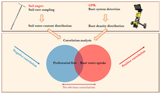
Abstract
:
1. Introduction
2. Materials and Methods
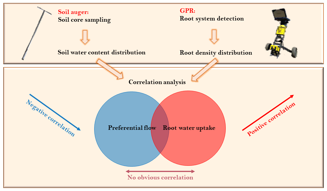
2.1. Study Site
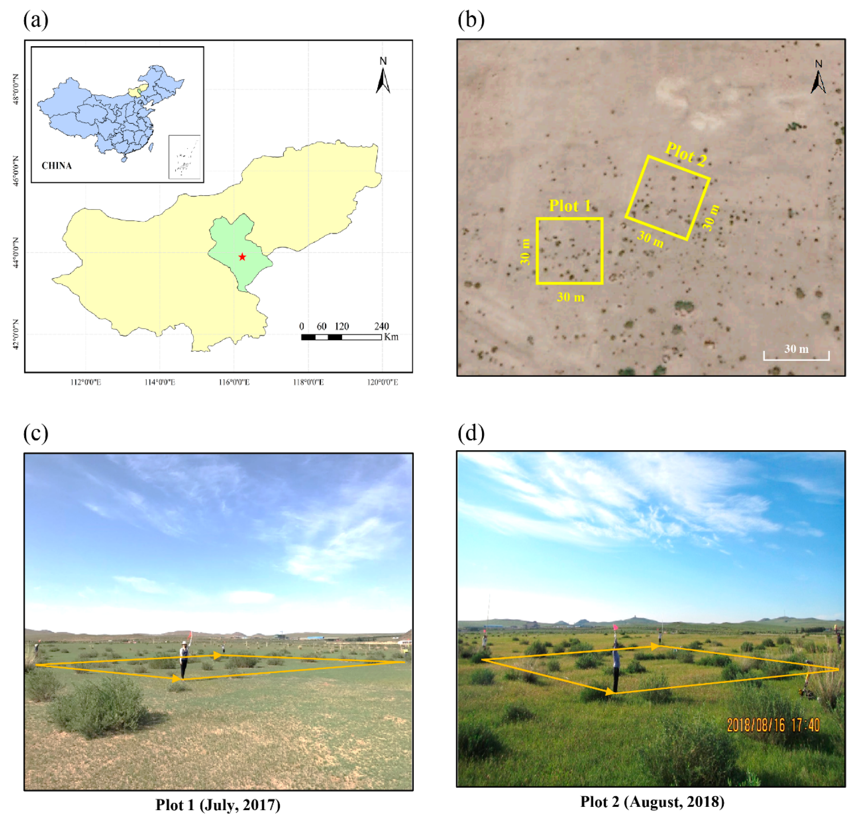
2.2. Field Experiment Design
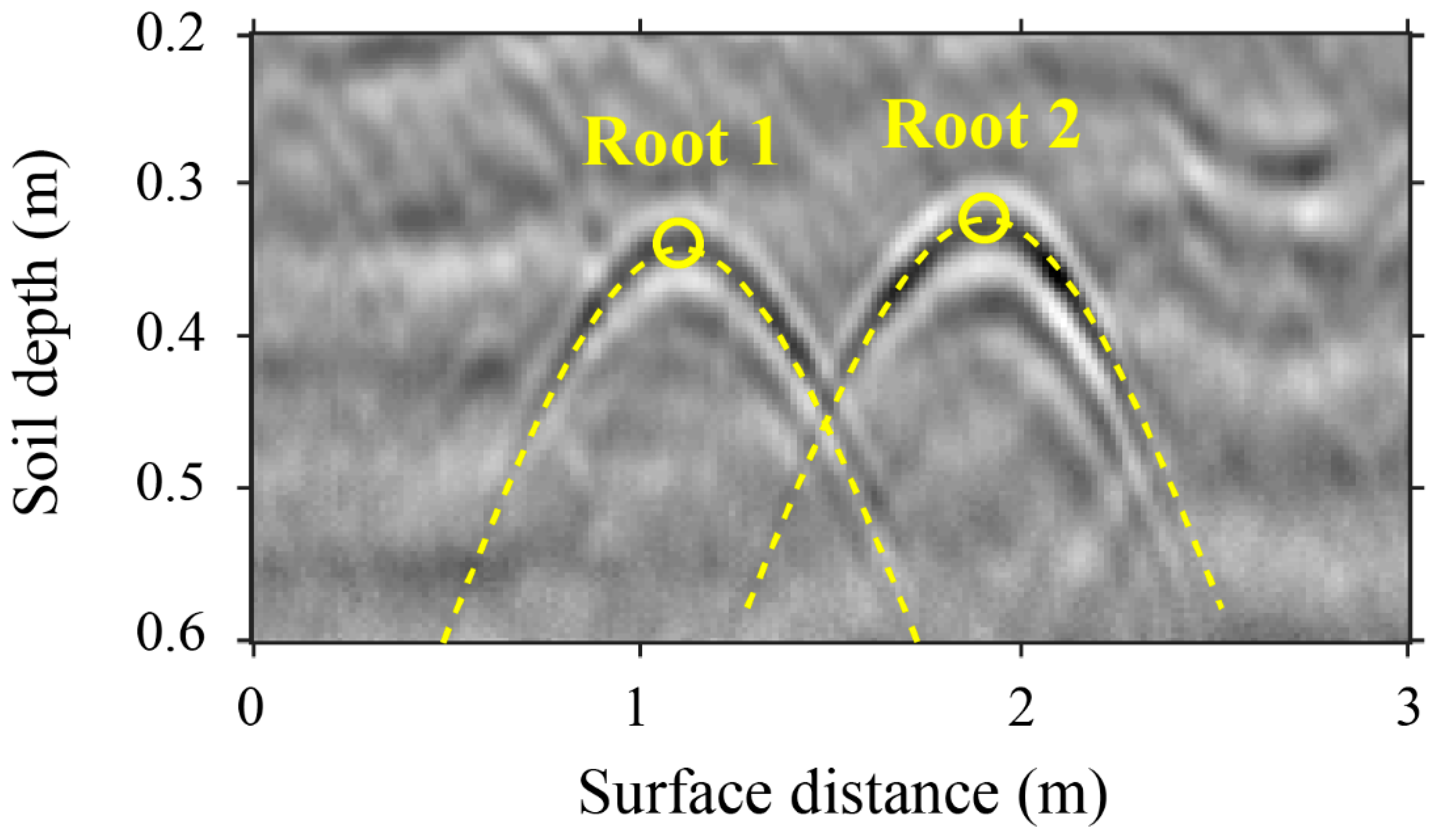
2.3. GPR Scanning and Processing
2.4. Root Points Cloud Reconstruction from GPR Data
2.5. SWC Measurement
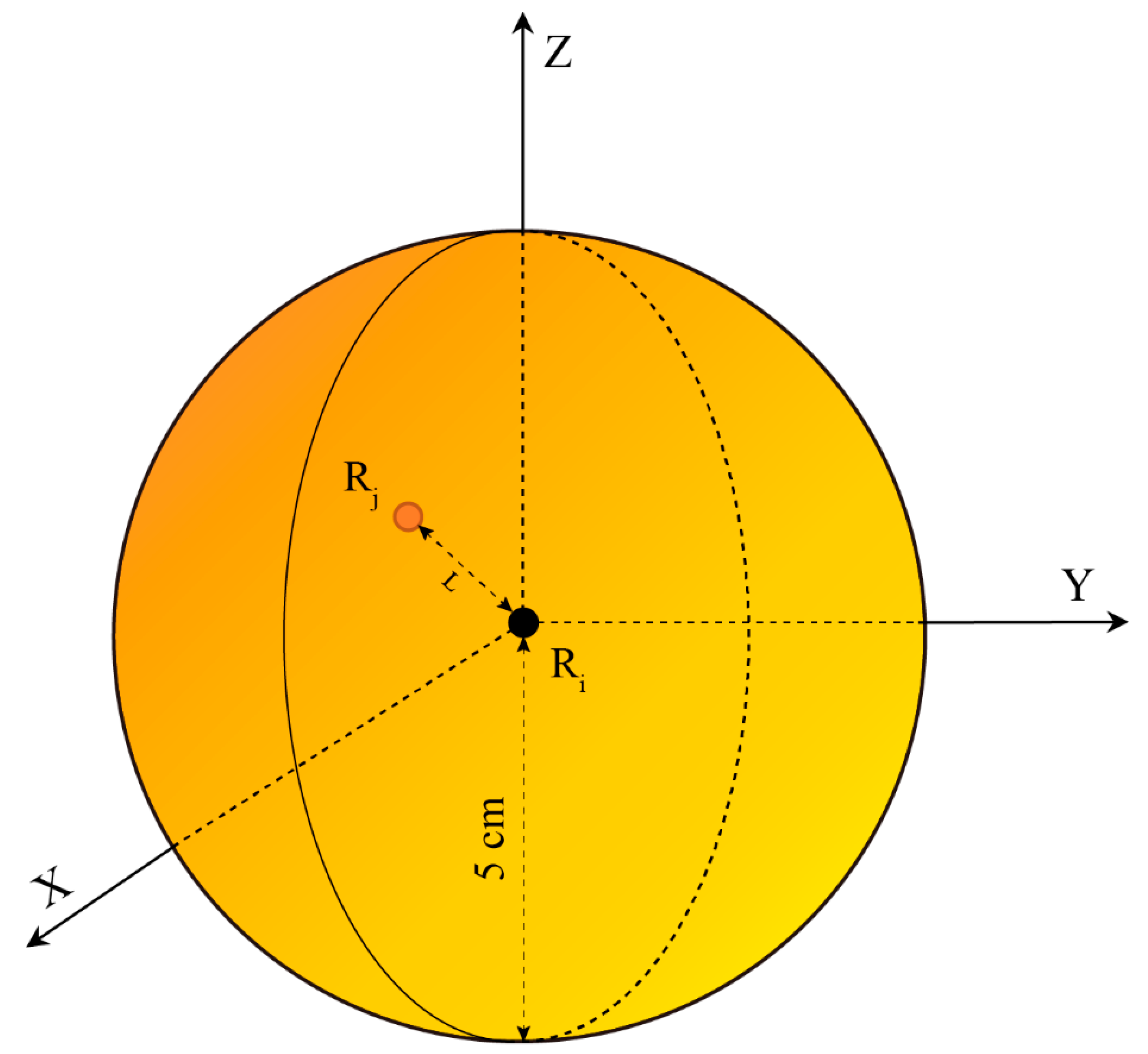
2.6. Exploring Root-Soil Water Relationship on Different Axes
2.7. Spatial Correlation between Root Distribution Density and SWC
3. Results
3.1. Vertical Distribution and Correlation of Roots and Soil Water
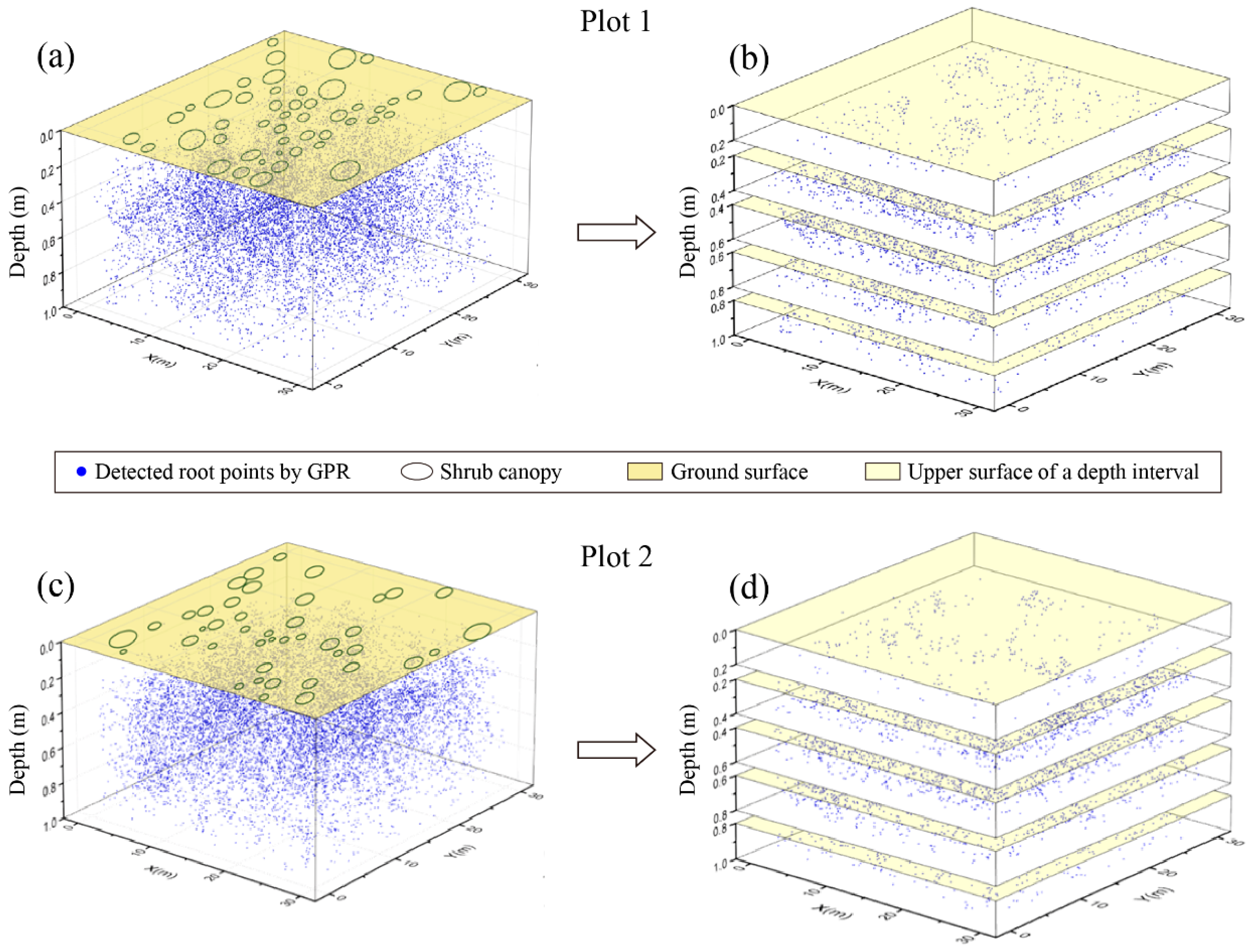
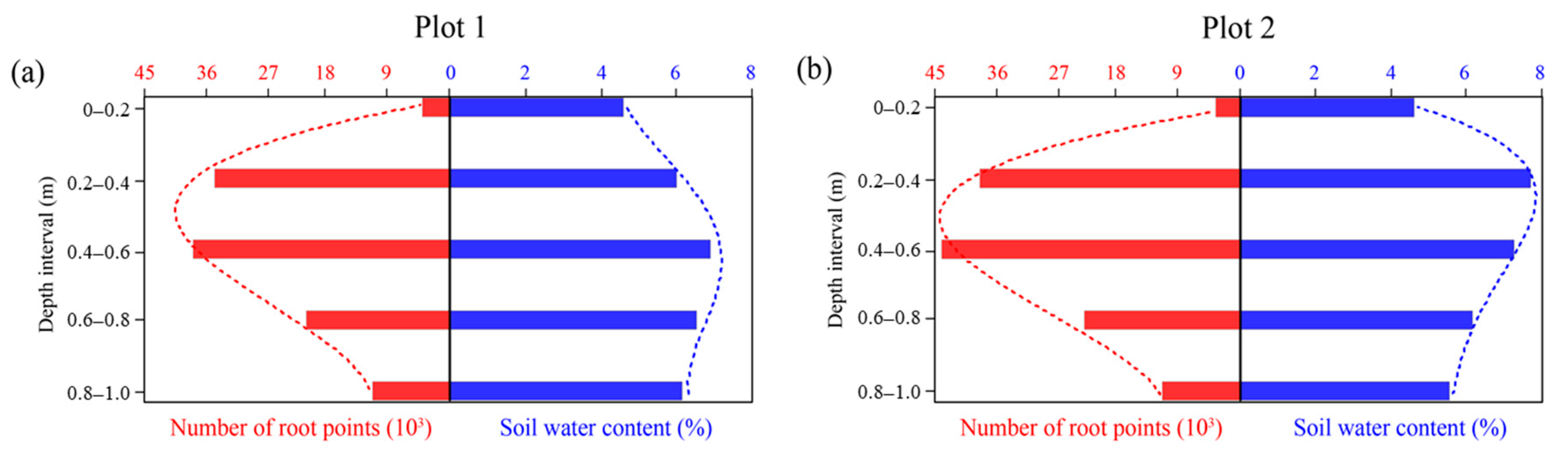
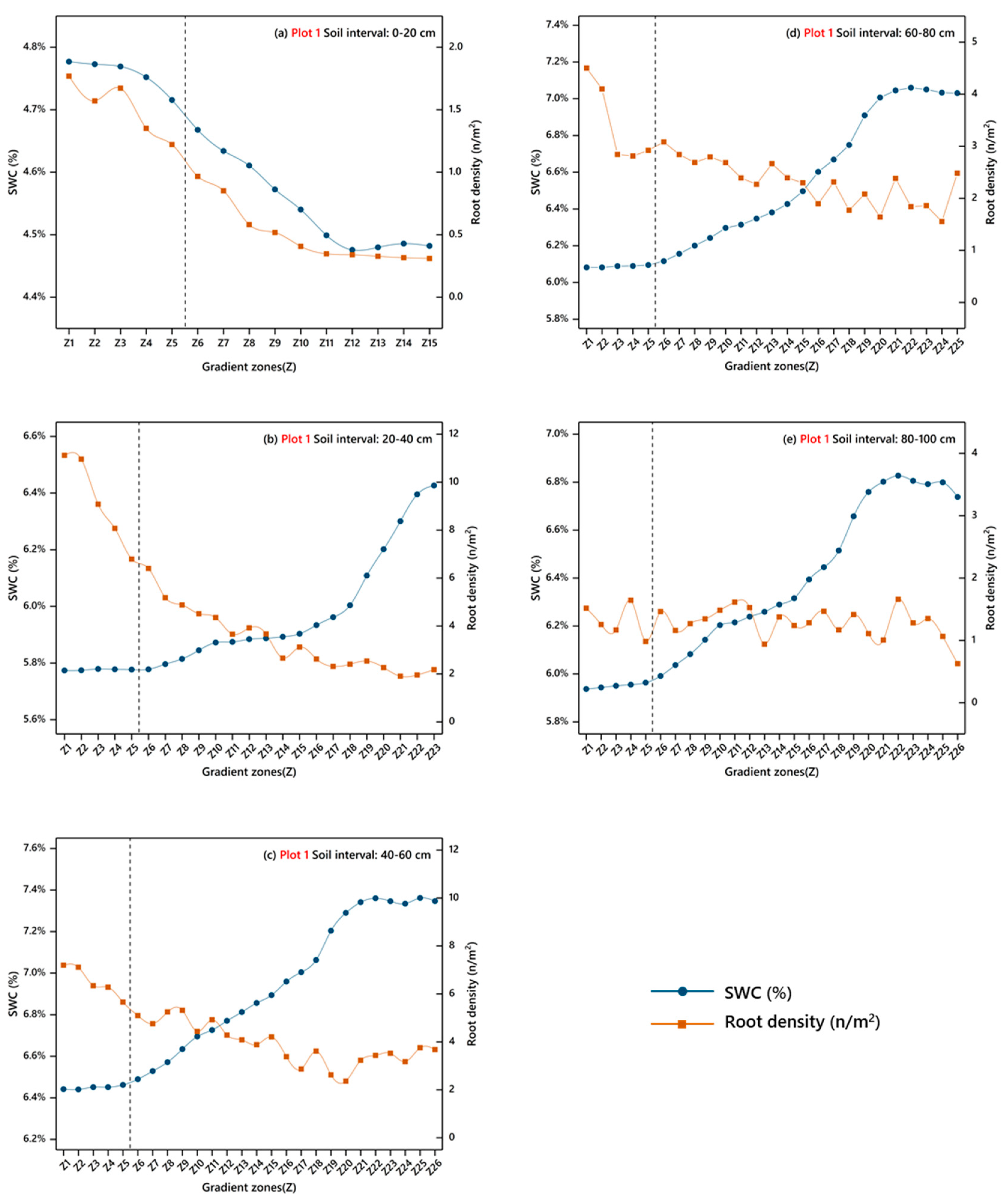
3.1.1. Distribution Pattern of Roots
3.1.2. Distribution Pattern of Soil Water
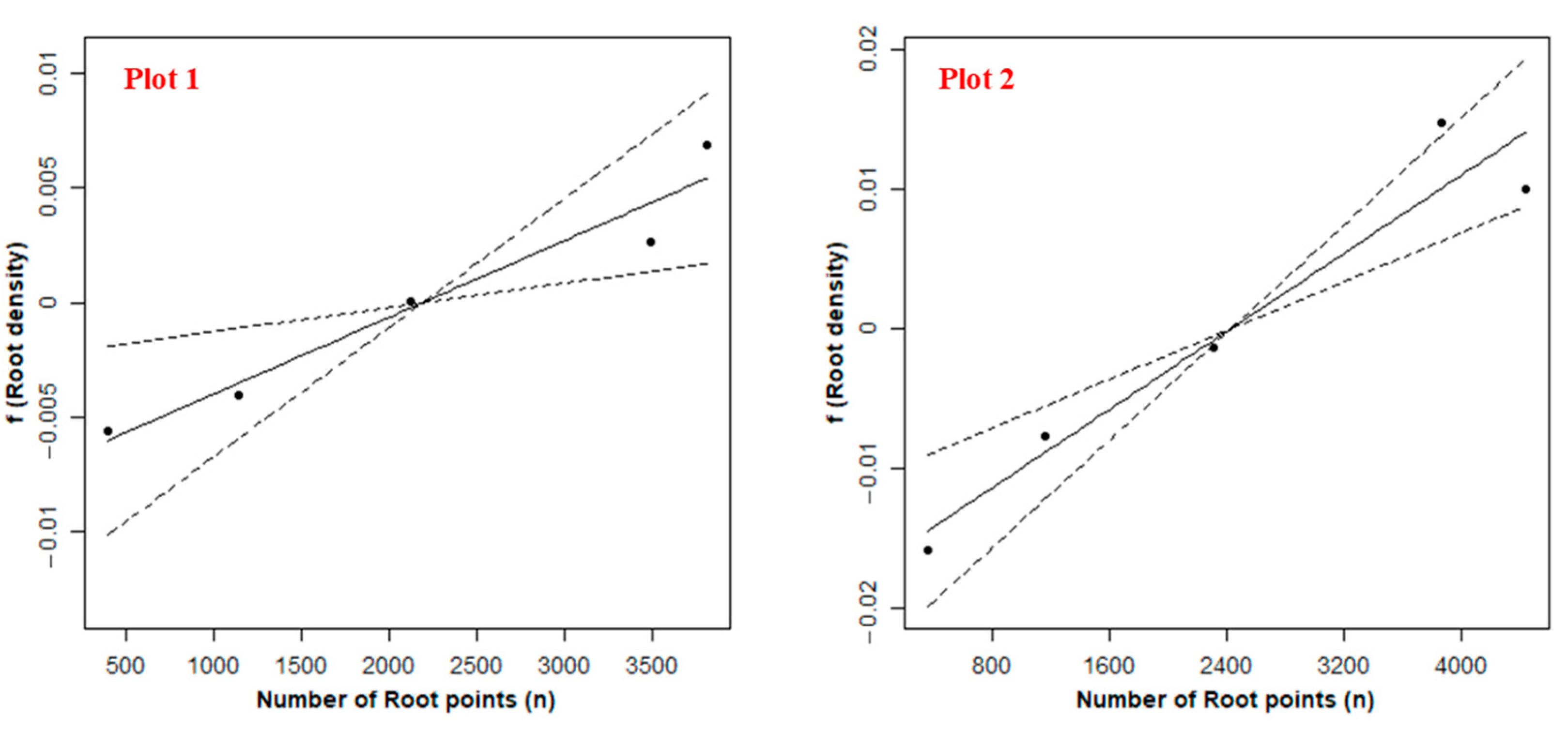
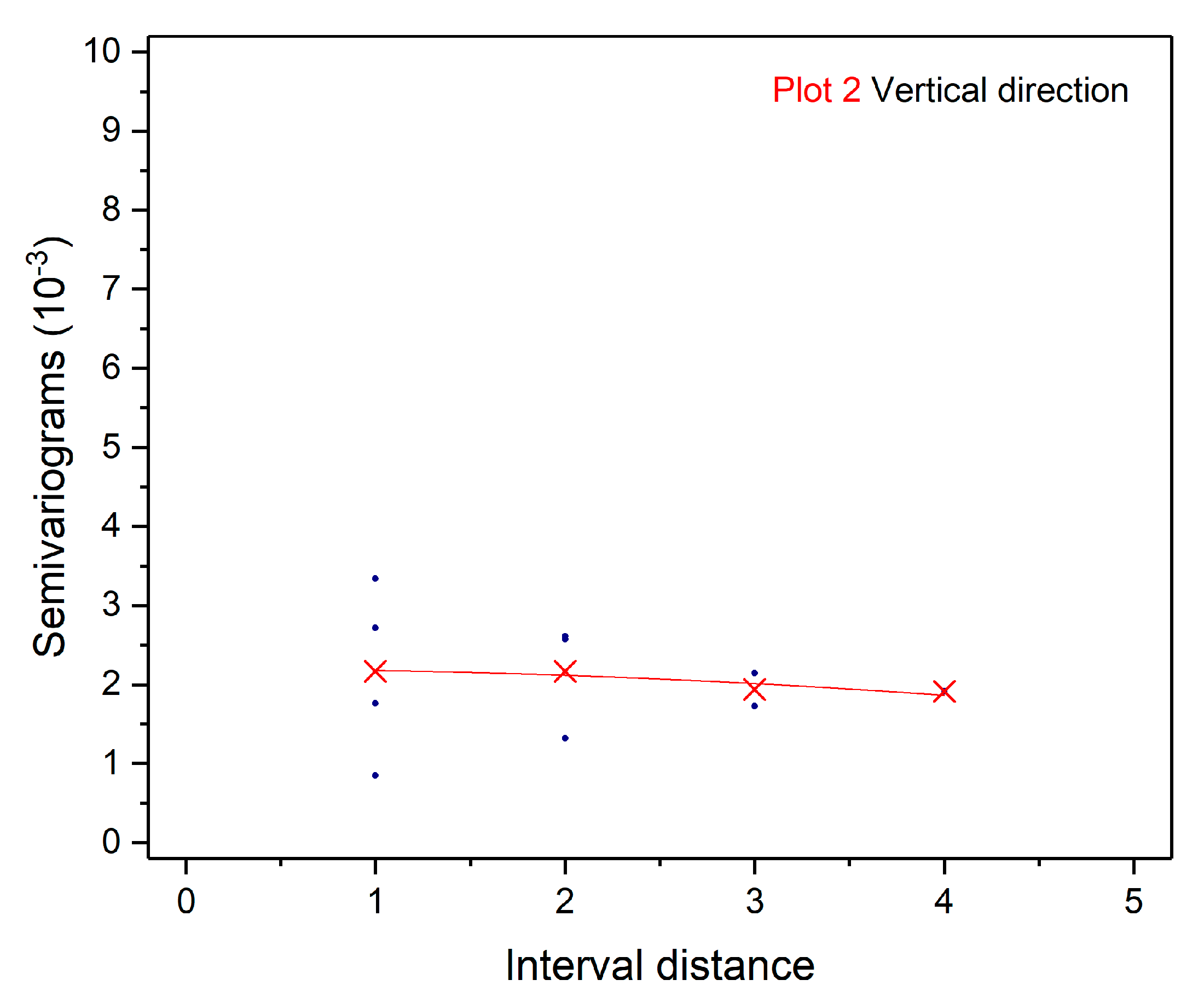
3.1.3. Correlation between Roots and Soil Water in the Vertical Direction
3.2. Horizontal Distribution and Correlation of Roots and Soil Water
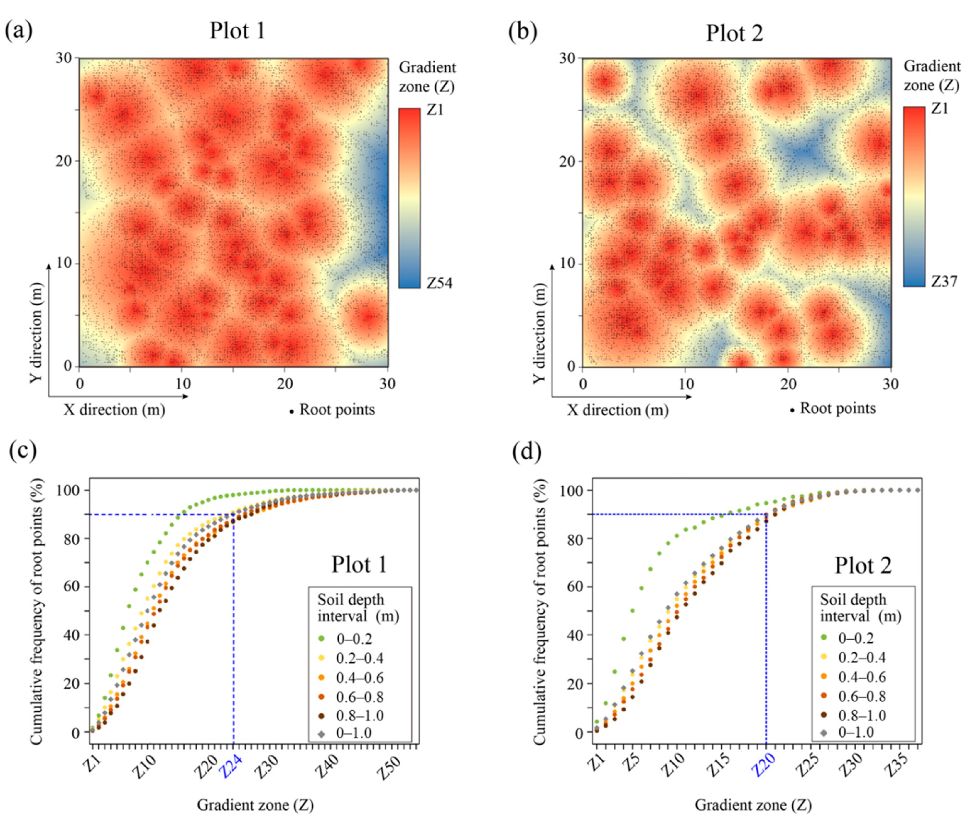
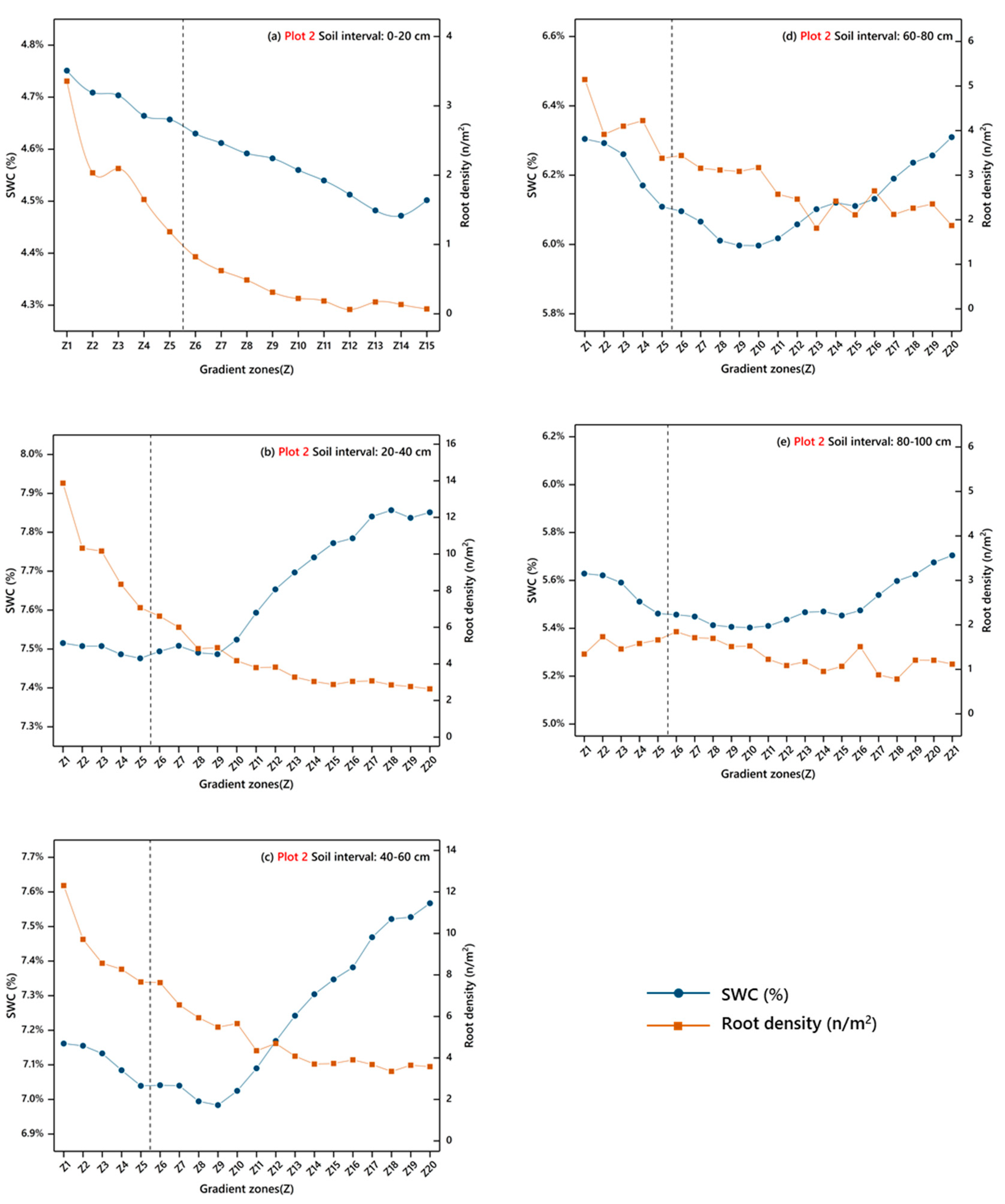
3.2.1. Distribution Pattern of Roots
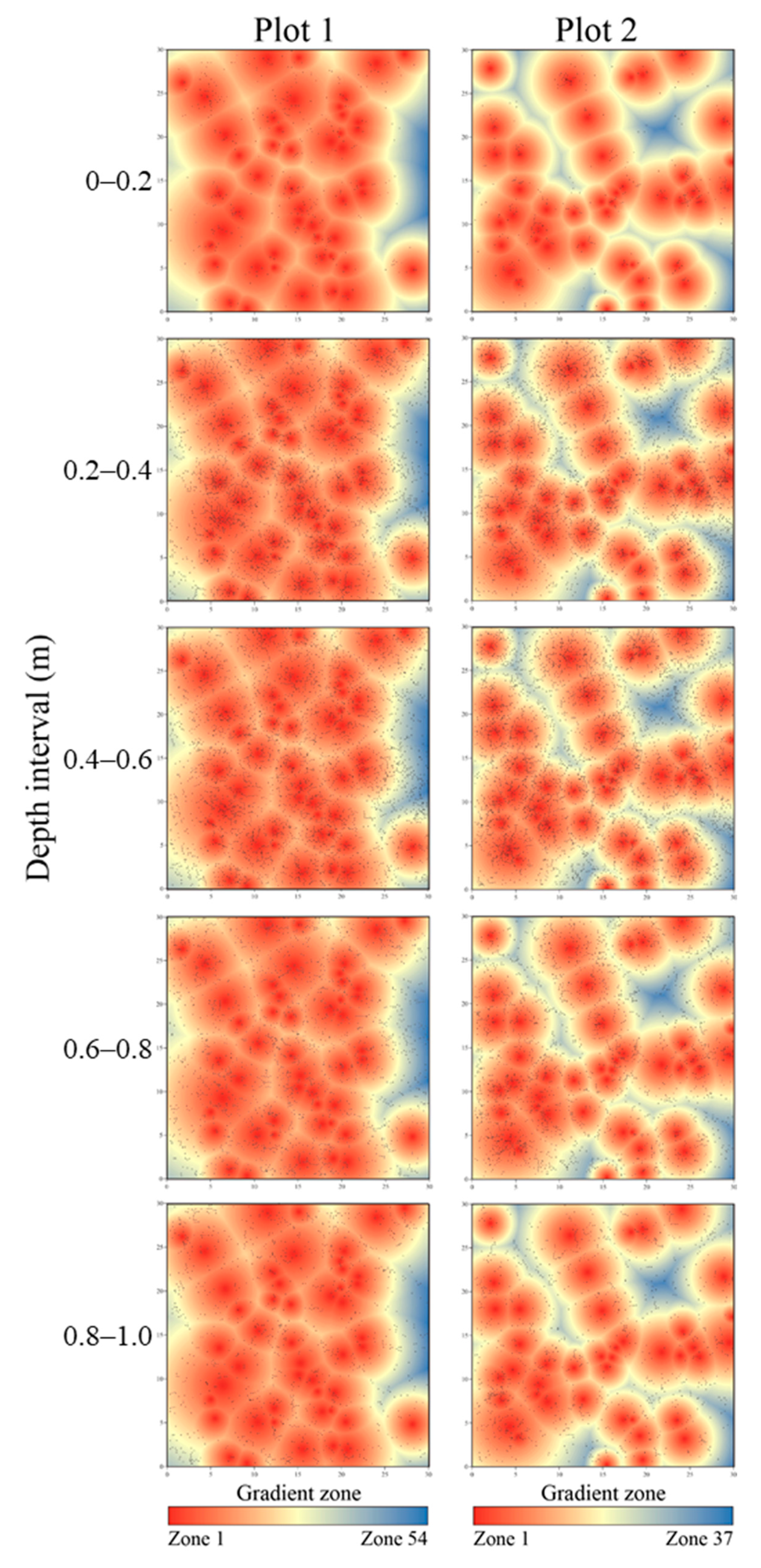
3.2.2. Distribution Pattern of Soil Water
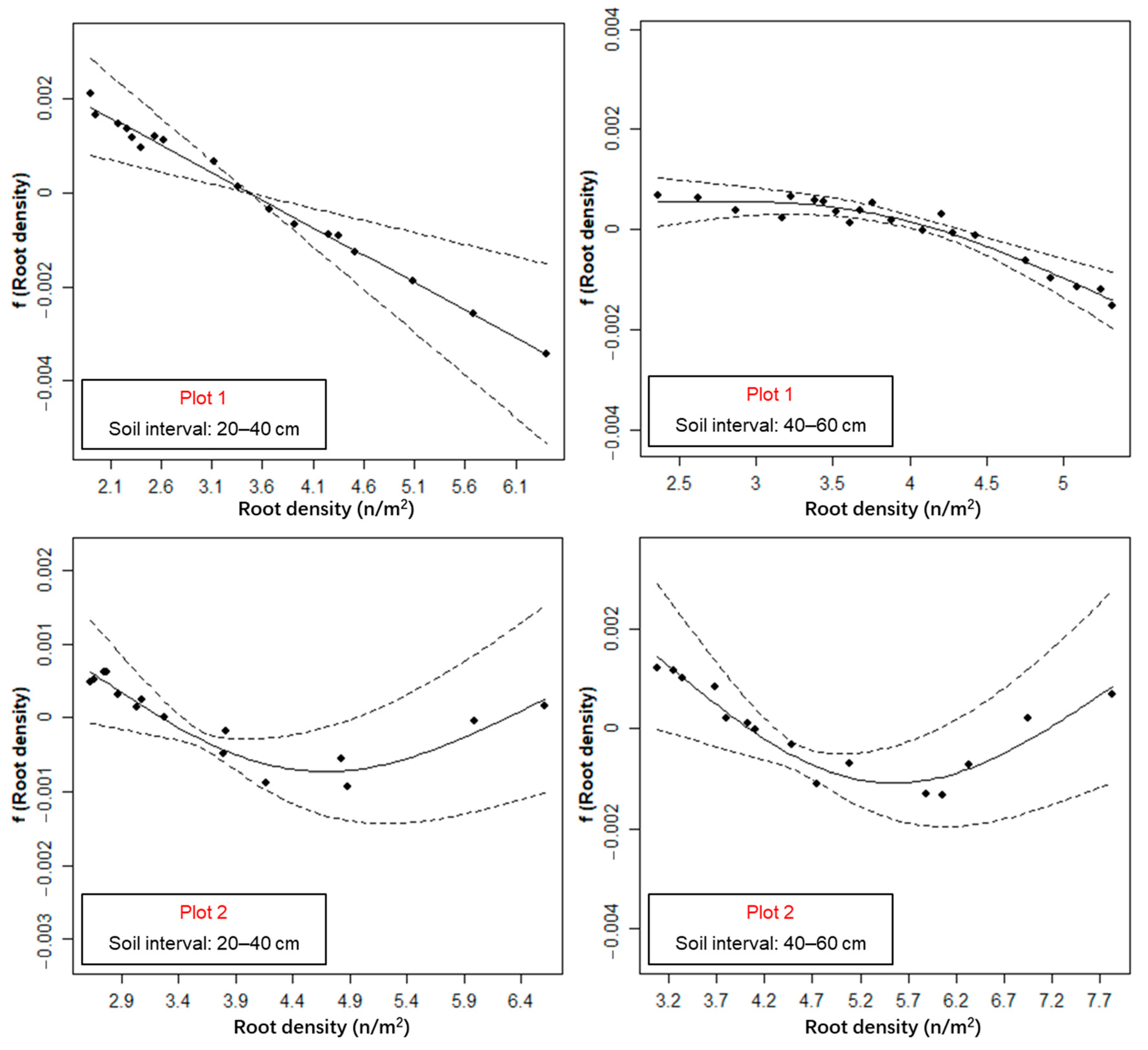
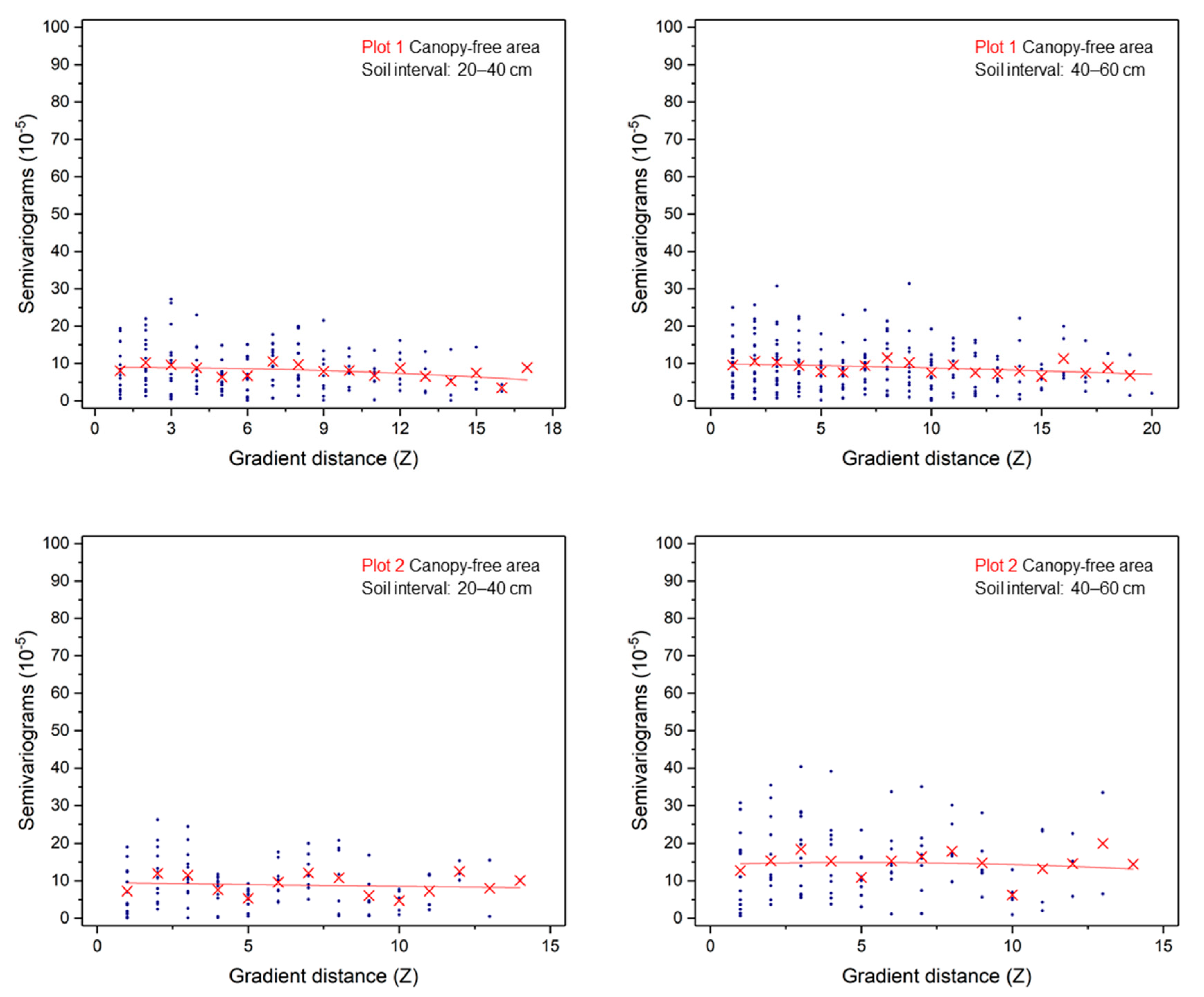
3.2.3. Correlation between Roots and Soil Water in the Horizontal Direction
4. Discussion
4.1. Root-Soil Water Relationship at the Study Site
4.2. Potentials and Limitations of the GPR Method in the Ecohydrological Study at Field Scales
5. Conclusions
Author Contributions
Funding
Data Availability Statement
Acknowledgments
Conflicts of Interest
Appendix A


References
- Chapin, F.S.; Vitousek, P.M.; Cleve, K.V. The Nature of Nutrient Limitation in Plant Communities. Am. Nat. 1986, 127, 48–58. [Google Scholar] [CrossRef]
- Kozlowski, T.T.; Pallardy, S.G. Acclimation and adaptive responses of woody plants to environmental stresses. Bot. Rev. 2002, 68, 270–334. [Google Scholar] [CrossRef]
- Snyman, H.A. Influence of water stress on root development of Opuntia ficus-indica and O. robusta. Arid Land Res. Manag. 2014, 28, 447–463. [Google Scholar] [CrossRef]
- Wu, M.; Zhang, W.; Ma, C.; Zhou, J. Changes in morphological, physiological, and biochemical responses to different levels of drought stress in Chinese cork oak (Quercus variabilis Bl.) seedlings. Russ. J. Plant Physiol. 2013, 60, 681–692. [Google Scholar] [CrossRef]
- Norman, J.M.; Anderson, M.C. Soil–plant–atmosphere continuum. In Encyclopedia of Soils in the Environment, 1st ed.; Hillel, D., Ed.; Elsevier: New York, NY, USA, 2005; pp. 513–521. [Google Scholar]
- Guo, L.; Lin, H. Critical zone research and observatories: Current status and future perspectives. Vadose Zone J. 2016, 15, 1–14. [Google Scholar] [CrossRef] [Green Version]
- Vereecken, H.; Huisman, J.A.; Bogena, H.; Vanderborght, J.; Vrugt, J.A.; Hopmans, J.W. On the value of soil moisture measurements in vadose zone hydrology: A review. Water Resour. Res. 2008, 44. [Google Scholar] [CrossRef] [Green Version]
- Li, H.; Wang, J.; Jiang, Z.; Ji, Y. Relationship between soil moisture and root biomass during developmental process of Nitraria tangutorum nebkha. J. Gansu Agr. Univ. 2010, 45, 133–138. [Google Scholar]
- Li, K.; Luo, Y.; Zhang, H.; She, H. The relations between root distribution of Artemisia halodendron and soil water in Horqin. J. Arid Land Resour. Environ. 2012, 26, 167–171. [Google Scholar]
- Yang, F. Study on the Characteristics of Salix psammophila Roots and Soil Moisture in Mu Us Sandy Land. J. Anhui Agric. Sci. 2011, 39, 16050–16052. [Google Scholar]
- Niu, H.; Li, H.; Zhao, M.; Han, X.; Dong, X. Relationship between soil water content and vertical distribution of root system under different ground water gradients in Maowusu Sandy Land. J. Arid Land Resour. Environ. 2008, 2, 157–163. [Google Scholar]
- Zhao, Y.; Yuan, W.; Sun, B.; Yang, Y.; Li, J.; Li, J.; Cao, B.; Zhong, H. Root distribution of three desert shrubs and soil moisture in Mu Us sand land. Res. Soil Water Conserv. 2010, 17, 129–133. [Google Scholar]
- Tobella, A.B.; Reese, H.; Almaw, A.; Bayala, J.; Malmer, A.; Laudon, H.; Ilstedt, U. The effect of trees on preferential flow and soil infiltrability in an agroforestry parkland in semi-arid Burkina Faso. Water Resour. Res. 2014, 50, 3342–3354. [Google Scholar] [CrossRef] [PubMed] [Green Version]
- Ceccon, C.; Panzacchi, P.; Scandellari, F.; Prandi, L.; Ventura, M.; Russo, B.; Millard, P.; Tagliavini, M. Spatial and temporal effects of soil temperature and moisture and the relation to fine root density on root and soil respiration in a mature apple orchard. Plant Soil. 2011, 342, 195–206. [Google Scholar] [CrossRef]
- Guo, L.; Mount, G.J.; Hudson, S.; Lin, H.; Levia, D. Pairing geophysical techniques improves understanding of the near-surface Critical Zone: Visualization of preferential routing of stemflow along coarse roots. Geoderma 2020, 357, 1–12. [Google Scholar] [CrossRef]
- Johnson, M.S.; Lehmann, J. Double-funneling of trees: Stemflow and root-induced preferential flow. Ecoscience 2006, 13, 324–333. [Google Scholar] [CrossRef]
- Li, L.; Zheng, X.; Li, X.; Zhang, S. Influences of Soil Infiltration and Preferential Flow by Shrub Caragana microphylla. J. Soil Water Conserv. 2015, 29, 55–59. [Google Scholar]
- Mitchell, A.R.; Ellsworth, T.R.; Meek, B.D. Effect of root systems on preferential flow in swelling soil. Commun. Soil Sci. Plant Anal. 1995, 26, 2655–2666. [Google Scholar] [CrossRef]
- Zhang, Y.; Niu, J.; Yu, X.; Zhu, W.; Du, X. Effects of fine root length density and root biomass on soil preferential flow in forest ecosystems. For. Syst. 2015, 24, 12. [Google Scholar] [CrossRef] [Green Version]
- Alamusa, J.D.; Pei, T. Soil moisture infiltration dynamics in plantation of Caragana microphylla in Heerqin sandy land. Chin. J. Ecol. 2004, 1, 56–59. [Google Scholar]
- Cheng, X.; Huang, M.; Shao, M. Relationship between fine roots distribution and soil water consumption of Populus simonii and Caragana korshinkii plantation on sandy land. Sci. Soil Water Conserv. 2008, 6, 77–83. [Google Scholar]
- Niu, C.; Liu, Y.A.; Guo, Y.; Tian, Y.; Wang, J.; Zhang, W. The characteristics of sand-fixation plantations roots and soil moisture in Horqin sandy land. J. Arid Land Resour. Environ. 2015, 10, 106–111. [Google Scholar]
- Alamusa, J.D.; Tiefan, P. Relationship between Root System Distribution and Soil Moisture of Artificial Caragana icrophylla Vegetation in Sandy Land. J. Soil Water Conserv. 2003, 17, 78–81. [Google Scholar]
- Wang, J.; Liu, M.; Sheng, S.; Xu, C.; Liu, X.; Wang, H. Spatial distributions of soil water, salts and roots in an arid arbor-herb community. Acta Ecol. Sin. 2008, 28, 4120–4127. [Google Scholar]
- Hruska, J.; Čermák, J.; Šustek, S. Mapping tree root systems with ground-penetrating radar. Tree Physiol. 1999, 19, 125–130. [Google Scholar] [CrossRef] [Green Version]
- Hagrey, S.A.A. Geophysical imaging of root-zone, trunk, and moisture heterogeneity. J. Exp. Bot. 2007, 58, 839–854. [Google Scholar] [CrossRef] [PubMed] [Green Version]
- Jayawickreme, D.H.; Jobbágy, E.G.; Jackson, R.B. Geophysical subsurface imaging for ecological applications. New Phytol. 2014, 201, 1170–1175. [Google Scholar] [CrossRef] [PubMed]
- Liu, Q.; Cui, X.; Liu, X.; Chen, J.; Chen, X.; Cao, X. Detection of root orientation using ground-penetrating radar. IEEE Trans. Geosci. Remote Sens. 2017, 56, 93–104. [Google Scholar] [CrossRef]
- Stokes, A.; Fourcaud, T.; Hruska, J.; Cermak, J.; Nadyezdhina, N.; Nadyezhdin, V.; Praus, L. An evaluation of different methods to investigate root system architecture of urban trees in situ: I. Ground-penetrating radar. J. Arboric. 2002, 28, 2–10. [Google Scholar]
- Cui, X.; Liu, X.; Cao, X.; Fan, B.; Zhang, Z.; Chen, J.; Chen, X.; Lin, H.; Guo, L. Pairing dual-frequency GPR in summer and winter enhances the detection and mapping of coarse roots in the semi-arid shrubland in China. Eur. J. Soil Sci. 2020, 71, 236–251. [Google Scholar] [CrossRef]
- Wu, Y.; Guo, L.; Cui, X.; Chen, J.; Cao, X.; Lin, H. Ground-penetrating radar-based automatic reconstruction of three-dimensional coarse root system architecture. Plant Soil. 2014, 383, 155–172. [Google Scholar] [CrossRef]
- Butnor, J.R.; Doolittle, J.; Johnsen, K.H.; Samuelson, L.; Stokes, T.; Kress, L. Utility of ground-penetrating radar as a root biomass survey tool in forest systems. Soil Sci. Soc. Am. J. 2003, 67, 1607–1615. [Google Scholar] [CrossRef] [Green Version]
- Butnor, J.R.; Doolittle, J.; Kress, L.; Cohen, S.; Johnsen, K.H. Use of ground-penetrating radar to study tree roots in the southeastern United States. Tree Physiol. 2001, 21, 1269–1278. [Google Scholar] [CrossRef] [PubMed] [Green Version]
- Cui, X.; Chen, J.; Shen, J.; Cao, X.; Chen, X.; Zhu, X. Modeling tree root diameter and biomass by ground-penetrating radar. Sci. China Earth Sci. 2011, 54, 711–719. [Google Scholar] [CrossRef]
- Cui, X.; Guo, L.; Chen, J.; Chen, X.; Zhu, X. Estimating tree-root biomass in different depths using ground-penetrating radar: Evidence from a controlled experiment. IEEE Trans. Geosci. Remote Sens. 2012, 51, 3410–3423. [Google Scholar] [CrossRef]
- Liu, X.; Cui, X.; Guo, L.; Chen, J.; Li, W.; Yang, D.; Cao, X.; Chen, X.; Liu, Q.; Lin, H. Non-invasive estimation of root zone soil moisture from coarse root reflections in ground-penetrating radar images. Plant Soil. 2019, 436, 623–639. [Google Scholar] [CrossRef]
- Guo, L.; Wu, Y.; Chen, J.; Hirano, Y.; Tanikawa, T.; Li, W.; Cui, X. Calibrating the impact of root orientation on root quantification using ground-penetrating radar. Plant Soil. 2015, 395, 289–305. [Google Scholar] [CrossRef]
- Hirano, Y.; Dannoura, M.; Aono, K.; Igarashi, T.; Ishii, M.; Yamase, K.; Makita, N.; Kanazawa, Y. Limiting factors in the detection of tree roots using ground-penetrating radar. Plant Soil. 2009, 319, 15–24. [Google Scholar] [CrossRef]
- Guo, L.; Lin, H.; Fan, B.; Cui, X.; Chen, J. Impact of root water content on root biomass estimation using ground penetrating radar: Evidence from forward simulations and field controlled experiments. Plant Soil. 2013, 371, 503–520. [Google Scholar] [CrossRef]
- Li, W.; Cui, X.; Guo, L.; Chen, J.; Chen, X.; Cao, X. Tree root automatic recognition in ground penetrating radar profiles based on randomized Hough transform. Remote Sens. 2016, 8, 430. [Google Scholar] [CrossRef] [Green Version]
- Zhang, T.; Su, Y.; Cui, J.; Zhang, Z.; Chang, X. A leguminous shrub (Caragana microphylla) in semi-arid sandy soils of north China. Pedosphere 2006, 16, 319–325. [Google Scholar] [CrossRef]
- Cao, C.; Jiang, D.; Luo, Y.; Kou, Z. Stability of Caragana microphylla plantation for wind protection and sand fixation. Acta Ecol. Sin. 2004, 24, 1178–1186. [Google Scholar]
- Ma, Z.; Shiyomi, M. Forty-eight-year climatology of air temperature and precipitation changes in Xilinhot, Xilingol steppe (Inner Mongolia), China. Grassl. Sci. 2011, 57, 168–172. [Google Scholar]
- Miao, H.; Chen, S.; Chen, J.; Zhang, W.; Zhang, P.; Wei, L.; Han, X.; Lin, G. Cultivation and grazing altered evapotranspiration and dynamics in Inner Mongolia steppes. Agr. For. Meteorol. 2009, 149, 1810–1819. [Google Scholar] [CrossRef]
- He, J. Precipitation variation characteristics of Xilinhot City for 50 years. Chin. Agric. Sci. Bull. 2012, 28, 271–278. [Google Scholar]
- Li, X.; Zhang, S.; Peng, H.; Hu, X.; Ma, Y. Soil water and temperature dynamics in shrub-encroached grasslands and climatic implications: Results from Inner Mongolia steppe ecosystem of north China. Agr. For. Meteorol. 2013, 171, 20–30. [Google Scholar] [CrossRef]
- IUSS Working Group WRB. World Reference Base for Soil Resources 2006, 2nd ed.; FAO (Food and Agriculture Organization of the United Nations): Roma, Italy, 2006; p. 128. [Google Scholar]
- Zhao, Y.; Peth, S.; Wang, X.; Lin, H.; Horn, R. Controls of surface soil moisture spatial patterns and their temporal stability in a semi-arid steppe. Hydrol. Process. 2010, 24, 2507–2519. [Google Scholar] [CrossRef]
- Cao, X.; Liu, Y.; Liu, Q.; Cui, X.; Chen, X.; Chen, J. Estimating the age and population structure of encroaching shrubs in arid/semi-arid grasslands using high spatial resolution remote sensing imagery. Remote Sens. Environ. 2018, 216, 572–585. [Google Scholar] [CrossRef]
- Guo, L.; Chen, J.; Cui, X.; Fan, B.; Lin, H. Application of ground penetrating radar for coarse root detection and quantification: A review. Plant Soil. 2013, 362, 1–23. [Google Scholar] [CrossRef] [Green Version]
- ESRI. ArcGIS Desktop: Release 10.2.2; Environmental Systems Research Institute: Redlands, CA, USA, 2014. [Google Scholar]
- Niu, X. Studies on the characteristics of Caragana root development and soma relevant physiology. Acta Bot. Boreali Occident. Sin. 2003, 23, 860–865. [Google Scholar]
- Yuan, J.; Tan, X.; Yuan, D.; Xie, P.; Jiang, Y. Study on root system distribution of Camellia oleifera. J. Zhejiang For. Sci. Technol. 2009, 29, 30–32. [Google Scholar]
- Zhang, Q.; Zhang, C.; Liu, M.; Yu, W.; Xu, C.; Wang, H. The influences of arboraceous layer on spatial patterns and morphological characteristics of herbaceous layer in an arid plant community. Acta Ecol. Sin. 2007, 27, 1265–1271. [Google Scholar]
- Lindh, B.C.; Gray, A.N.; Spies, T.A. Responses of herbs and shrubs to reduced root competition under canopies and in gaps: A trenching experiment in old-growth Douglas-fir forests. Can. J. For. Res. 2003, 33, 2052–2057. [Google Scholar] [CrossRef] [Green Version]
- Vetaas, O.R. Micro-site effects of trees and shrubs in dry savannas. J. Veg. Sci. 1992, 3, 337–344. [Google Scholar] [CrossRef]
- Moreno-Fernández, D.; Álvarez-González, J.G.; Rodríguez-Soalleiro, R.; Pasalodos-Tato, M.; Pérez-Cruzado, C. National-scale assessment of forest site productivity in spain. For. Ecol. Manag. 2018, 417, 197–207. [Google Scholar] [CrossRef]
- Wood, S.N. Thin plate regression splines. J. Roy. Stat. Soc. 2003, 65, 95–114. [Google Scholar] [CrossRef]
- R Core Team. R: A Language and Environment for Statistical Computing; R Foundation for Statistical Computing: Vienna, Austria, 2017. [Google Scholar]
- Guo, Y.; Qi, W. Correlations between roots of Caragana korshinskii and soil moisture after stumping. Ekoloji 2018, 27, 9–20. [Google Scholar]
- Wang, S.; Zhao, X.; Zuo, X.; Zhao, W.; Guo, Y. Spatial Variability of the Response of Soil Moisture Content under Caragana Microphylla Shrubbery to Rainfall in the Horqin Sand Land. Arid Zone Res. 2008, 25, 389–393. [Google Scholar]
- Guo, L.; Lin, H. Addressing two bottlenecks to advance the understanding of preferential flow in soils. Adv. Agron. 2018, 147, 61–117. [Google Scholar]
- Davis, C.H. Absorption of soil moisture by maize roots. Bot. Gaz. 1940, 101, 791–805. [Google Scholar] [CrossRef]
- Leuschner, C.; Coners, H.; Icke, R. In situ measurement of water absorption by fine roots of three temperate trees: Species differences and differential activity of superficial and deep roots. Tree Physiol. 2004, 24, 1359–1367. [Google Scholar] [CrossRef] [PubMed] [Green Version]
- Cao, Y.; Ding, J.; Yu, Y.; Huang, G. Preliminary Studies on Haloxylon Ammodendron ‘Fertile Islands’ in Desert Soils Different in Texture. Acta Geol. Sin. 2016, 53, 261–270. [Google Scholar]
- Huang, T.; Tang, L.; Chen, L.; Zhang, Q. Root architecture and ecological adaptation strategy of three shrubs in karst area. Sci. Soil Water Conserv. 2019, 17, 89–94. [Google Scholar]
- Caldwell, M.M.; Richards, J.H. Hydraulic lift: Water efflux from upper roots improves effectiveness of water uptake by deep roots. Oecologia 1989, 79, 1–5. [Google Scholar] [CrossRef] [PubMed]
- Eapen, D.; Barroso, M.L.; Ponce, G.; Campos, M.E.; Cassab, G.I. Hydrotropism: Root growth responses to water. Trends Plant Sci. 2005, 10, 44–50. [Google Scholar] [CrossRef]
- Zhang, J.; Han, H.; Lei, Y.; Yang, W.; Li, Y.; Yang, D.; Zhao, X. Correlations between distribution characteristics of Artemisia ordosica root system and soil moisture under different fixation stage of sand dunes. J. Southwest For. Univ. 2012, 32, 1–5. [Google Scholar]
- Butnor, J.R.; Samuelson, L.J.; Stokes, T.A.; Johnsen, K.H.; Anderson, P.H.; González-Benecke, C.A. Surface-based GPR underestimates below-stump root biomass. Plant Soil. 2016, 402, 47–62. [Google Scholar] [CrossRef]
- Burns, I.G. Influence of the spatial distribution of nitrate on the uptake of N by plants: A review and a model for rooting depth. Eur. J. Soil Sci. 1980, 31, 155–173. [Google Scholar] [CrossRef]
- Giehl, R.F.; Gruber, B.D.; von Wirén, N. It’s time to make changes: Modulation of root system architecture by nutrient signals. J. Exp. Bot. 2014, 65, 769–778. [Google Scholar] [CrossRef]
- Hodge, A. The plastic plant: Root responses to heterogeneous supplies of nutrients. New Phytol. 2004, 162, 9–24. [Google Scholar] [CrossRef]
- Cahill, J.F.; McNickle, G.G.; Haag, J.J.; Lamb, E.G.; Nyanumba, S.M.; Clair, C.C.S. Plants integrate information about nutrients and neighbors. Science 2010, 328, 1657. [Google Scholar] [CrossRef] [Green Version]
- Stevens, G.N.; Jones, R.H. Patterns in soil fertility and root herbivory interact to influence fine-root dynamics. Ecology 2006, 87, 616–624. [Google Scholar] [CrossRef] [PubMed] [Green Version]


| Number of Shrubs | The Maximum of the Canopy’s Long Diameter | The Minimum of the Canopy’s Long Diameter | The Mean of the Canopy’s Long Diameter | |
|---|---|---|---|---|
| Plot 1 | 48 | 2.9 m | 0.3 m | 1.5525 m |
| Plot 2 | 42 | 3.3 m | 0.5 m | 1.7619 m |
| Plots | Intercept | f(I) | f(N) | Deviance (%) |
|---|---|---|---|---|
| 2017 | <0.01 | <0.05 | n.s. a | 98.3 |
| 2018 | <0.01 | n.s. | <0.05 | 93.4 |
| Plot 1 | Plot 2 | |||||
|---|---|---|---|---|---|---|
| Depth (cm) | Zone 1 | Zone 2 | Zone 3 | Zone 1 | Zone 2 | Zone 3 |
| 0–20 | Z1–Z5 | Z6–Z15 | Z16–Z54 | Z1–Z5 | Z6–Z15 | Z16–Z37 |
| 20–40 | Z1–Z5 | Z6–Z23 | Z24–Z54 | Z1–Z5 | Z6–Z20 | Z21–Z37 |
| 40–60 | Z1–Z5 | Z6–Z26 | Z27–Z54 | Z1–Z5 | Z6–Z20 | Z21–Z37 |
| 60–80 | Z1–Z5 | Z6–Z25 | Z26–Z54 | Z1–Z5 | Z6–Z20 | Z21–Z37 |
| 80–100 | Z1–Z5 | Z6–Z26 | Z27–Z54 | Z1–Z5 | Z6–Z21 | Z22–Z37 |
| Plots & Zones | Depth(m) | Intercept | f(Z) | f(ρ) | Deviance (%) |
|---|---|---|---|---|---|
| Plot1 Canopy-free | 0–0.2 | <0.01 | <0.05 | n.s. a | 99.4 |
| 0.2–0.4 | <0.01 | <0.01 | <0.05 | 99.0 | |
| 0.4–0.6 | <0.01 | <0.01 | <0.01 | 99.8 | |
| 0.6–0.8 | <0.01 | <0.01 | n.s. | 99.8 | |
| 0.8–1.0 | <0.01 | <0.01 | n.s. | 99.9 | |
| Plot2 Canopy-free | 0–0.2 | <0.01 | <0.01 | n.s. | 96.9 |
| 0.2–0.4 | <0.01 | <0.05 | <0.01 | 99.0 | |
| 0.4–0.6 | <0.01 | <0.05 | <0.01 | 98.7 | |
| 0.6–0.8 | <0.01 | <0.01 | n.s. | 94.8 | |
| 0.8–1.0 | <0.01 | <0.01 | n.s. | 98.0 |
Publisher’s Note: MDPI stays neutral with regard to jurisdictional claims in published maps and institutional affiliations. |
© 2021 by the authors. Licensee MDPI, Basel, Switzerland. This article is an open access article distributed under the terms and conditions of the Creative Commons Attribution (CC BY) license (http://creativecommons.org/licenses/by/4.0/).
Share and Cite
Cui, X.; Zhang, Z.; Guo, L.; Liu, X.; Quan, Z.; Cao, X.; Chen, X. The Root-Soil Water Relationship Is Spatially Anisotropic in Shrub-Encroached Grassland in North China: Evidence from GPR Investigation. Remote Sens. 2021, 13, 1137. https://0-doi-org.brum.beds.ac.uk/10.3390/rs13061137
Cui X, Zhang Z, Guo L, Liu X, Quan Z, Cao X, Chen X. The Root-Soil Water Relationship Is Spatially Anisotropic in Shrub-Encroached Grassland in North China: Evidence from GPR Investigation. Remote Sensing. 2021; 13(6):1137. https://0-doi-org.brum.beds.ac.uk/10.3390/rs13061137
Chicago/Turabian StyleCui, Xihong, Zheng Zhang, Li Guo, Xinbo Liu, Zhenxian Quan, Xin Cao, and Xuehong Chen. 2021. "The Root-Soil Water Relationship Is Spatially Anisotropic in Shrub-Encroached Grassland in North China: Evidence from GPR Investigation" Remote Sensing 13, no. 6: 1137. https://0-doi-org.brum.beds.ac.uk/10.3390/rs13061137