Article

Assessing the Effect of Drought on Winter Wheat Growth Using Unmanned Aerial System (UAS)-Based Phenotyping

1
Texas A&M AgriLife Research and Extension Center, Corpus Christi, TX 78406, USA
2
Texas A&M AgriLife Research and Extension Center, Amarillo, TX 79106, USA
3
Department of Soil and Crop Sciences, Texas A&M University, College Station, TX 77843, USA
4
School of Engineering and Computing Sciences, Texas A&M University-Corpus Christi, Corpus Christi, TX 78412, USA
5
Lyles School of Civil Engineering, Purdue University, West Lafayette, IN 47907, USA
*
Author to whom correspondence should be addressed.
Submission received: 24 January 2021 / Revised: 9 March 2021 / Accepted: 12 March 2021 / Published: 17 March 2021
(This article belongs to the Special Issue Remote Sensing in Assessing Responses of Vegetation to Drought)

Abstract

:
Drought significantly limits wheat productivity across the temporal and spatial domains. Unmanned Aerial Systems (UAS) has become an indispensable tool to collect refined spatial and high temporal resolution imagery data. A 2-year field study was conducted in 2018 and 2019 to determine the temporal effects of drought on canopy growth of winter wheat. Weekly UAS data were collected using red, green, and blue (RGB) and multispectral (MS) sensors over a yield trial consisting of 22 winter wheat cultivars in both irrigated and dryland environments. Raw-images were processed to compute canopy features such as canopy cover (CC) and canopy height (CH), and vegetation indices (VIs) such as Normalized Difference Vegetation Index (NDVI), Excess Green Index (ExG), and Normalized Difference Red-edge Index (NDRE). The drought was more severe in 2018 than in 2019 and the effects of growth differences across years and irrigation levels were visible in the UAS measurements. CC, CH, and VIs, measured during grain filling, were positively correlated with grain yield (r = 0.4–0.7, p < 0.05) in the dryland in both years. Yield was positively correlated with VIs in 2018 (r = 0.45–0.55, p < 0.05) in the irrigated environment, but the correlations were non-significant in 2019 (r = 0.1 to −0.4), except for CH. The study shows that high-throughput UAS data can be used to monitor the drought effects on wheat growth and productivity across the temporal and spatial domains.

1. Introduction

Wheat (Triticum aestivum L.) is the second most important crop in Texas, after cotton (Gossypium spp.), where it is produced under dryland and irrigated conditions for grain and forage. In 2020, it was planted on 1.9 million hectares, of which 0.97 million hectares were harvested for grain with a total production of 16 million Mt [1]. The frequent occurrence of drought poses a threat to winter wheat production in this region and reduces the yield under both the dryland and irrigated conditions [2]. The historic drought of 2011 and 2012 reduced wheat yield in Texas to 1.2 Mt compared to the five-year average of 2.5 Mt per hectare [3]. Another drought episode followed in 2018 when precipitation dropped below 150 mm. The frequent and unpredictable magnitude of drought observed this past decade reinforces the need to prepare for future climate threats.
Development of drought-tolerant cultivars along with better water management strategies can help reduce the impact of drought [4]. However, drought tolerance is a complex trait and cannot be easily measured [5]. Several physiological factors have been studied to identify genotypes that maintain yield stability across drought-prone environments [6,7]. Lower canopy temperature [8,9], induced by higher stomatal conductance, stay-green to prolong grain fill [10], seedling vigor to achieve early season ground cover, and root architecture [11] are some of the traits used to understand the physiological basis of drought tolerance in wheat. Although these traits provide insight into genotype performance, there remains uncertainty regarding the stability and interactivity of the traits. For example, early vigor, which is defined as rapid early growth and accumulation of above-ground biomass, has a positive relationship with the final grain yield in wheat. This is achieved by reducing evaporation and weed competition [12,13,14]. However, this may not always be true under drought conditions since more growth and biomass accumulation early in the season may reduce soil moisture available for anthesis and grain fill [15] leading to reduction in seed number and seed size [16]. Therefore, it is important to integrate multiple traits when developing selection criteria for breeding drought tolerant wheat varieties. Data must be collected throughout the growing season to fully understand the seasonal dynamics of traits and their interactions. Tools and techniques to assess early season drought impacts can assist producers to make crop management decisions and the same tools can help crop breeders to develop drought-tolerant cultivars.
Various methods have been proposed to monitor the effect of drought on wheat production. Liu et al. [17] evaluated palmer drought severity index (PDSI), standardized precipitation index (SPI), and standardized precipitation evapotranspiration index (SPEI) to compare the strength of these indices for drought assessment. Tigkas and Tsakiris [18] used the Reconnaissance Drought Index (RDI) to make early predictions of wheat yield under drought and found a reasonable prediction accuracy. Although useful, these indices are highly based on meteorological data. Indices developed by comparing yield in dryland with yield in irrigated environments is commonly used by breeders to evaluate the yield stability of genotypes [19]. Additional methods include ground-based point observations of some biophysical parameters such as soil moisture [20], leaf water potential [21,22], photosynthesis, and water use efficiency [23,24,25,26], but these measurements are cumbersome and time consuming. Vegetation indices (VIs) such as Normalized Difference Vegetation Index (NDVI) [27,28], Enhanced Vegetation Index (EVI) [27], Vegetation Condition Index (VCI) [29,30,31] obtained from satellite imagery have been used to assess the effect of drought on multiple crops. However, satellite remote sensing has limited spatial and temporal resolutions and cloud coverage can interfere with data collection in small breeding plots. Recent advancements in sensor and Unmanned Aerial System (UAS) technology has the potential to overcome the limitations of satellite imagery [32].
The use of UAS-based High-Throughput Phenotyping (HTP) is rapidly evolving as a useful tool to collect high-spatiotemporal data [33]. A single sensor attached to an Unmanned Aerial Vehicle (UAV) can collect data on many phenotypes in a relatively shorter time. In this research, we studied the seasonal dynamics of canopy cover (CC), canopy height (CH), NDVI, Excess Green Index (ExG), and Normalized Difference Red-edge Index (NDRE) obtained from UAS to assess the effect of drought on winter wheat growth. CC measures the percentage of green canopy and is positively correlated with leaf area index in wheat [34]. VIs are used to estimate several phenotypic features. For example, Bhandari et al. [35] used NDVI and other VIs to quantify leaf rust (Puccinia triticina f. sp. Tritici) severity in wheat. Hassan et al. [36] and Serrano et al. [37] showed a positive relationship of NDVI with biomass and grain yield in wheat. Potgieter et al. [38] and Barnhart et al. [39] used NDRE to characterize the leaf area and senescence patterns of sorghum (Sorghum bicolor). ExG measures the intensity of the greenness of the canopy by utilizing the normalized visible spectrum. Except for CH, the canopy features are dependent on the amount of chlorophyll present in the leaves [40]. Drought significantly reduces leaf chlorophyll content, photosynthesis, and other plant attributes, resulting in canopy deterioration, stunted growth [41], and ultimately reduced yield. This study is a part of an ongoing project to integrate a UAS-based HTP system into the Texas A&M’s winter wheat breeding program. The major objectives of this study are to (i) assess the impact of drought on winter wheat growth based on multi-temporal UAS-based canopy features, (ii) outline the procedure of UAS data collection, processing, and extraction, and (iii) determine the relationships between grain yield and UAS-based canopy features.

2. Materials and Methods
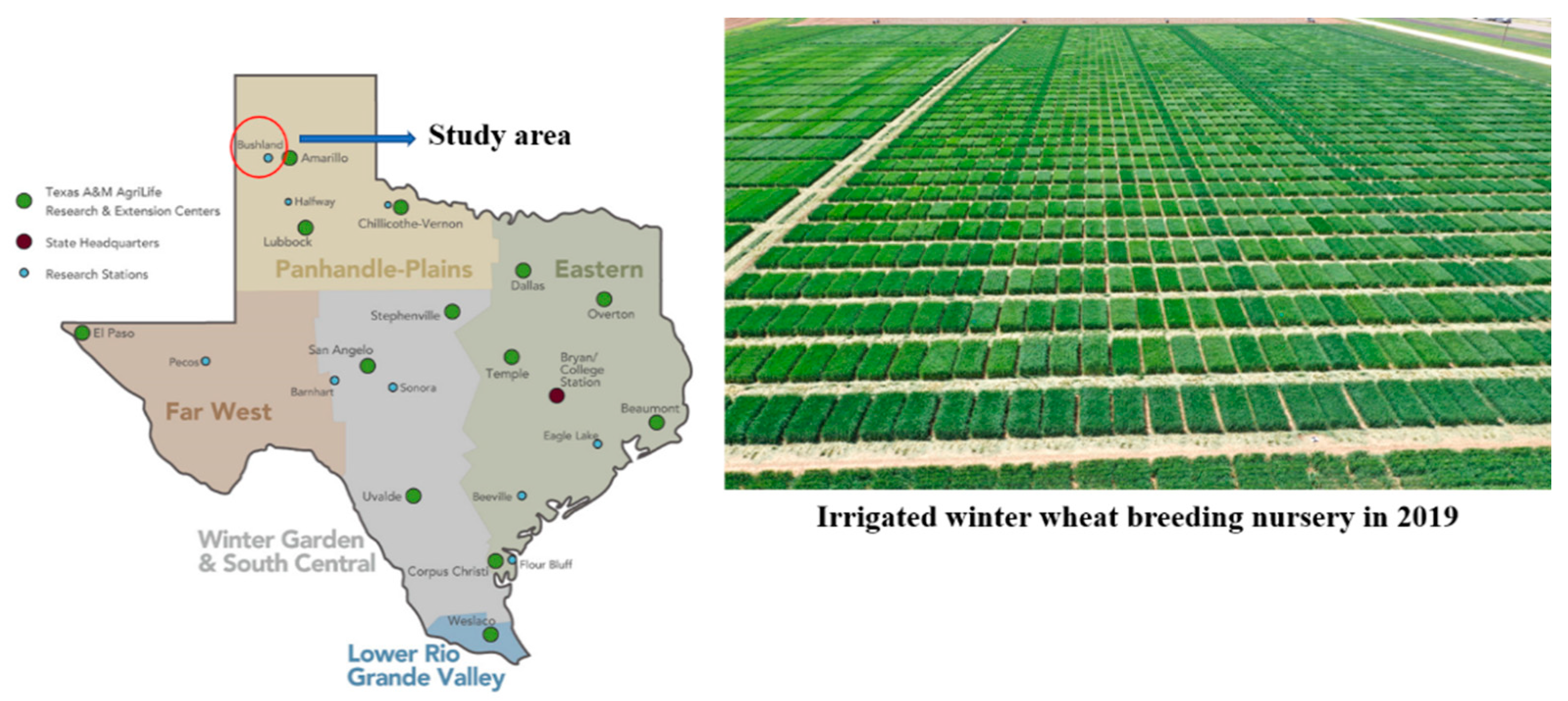
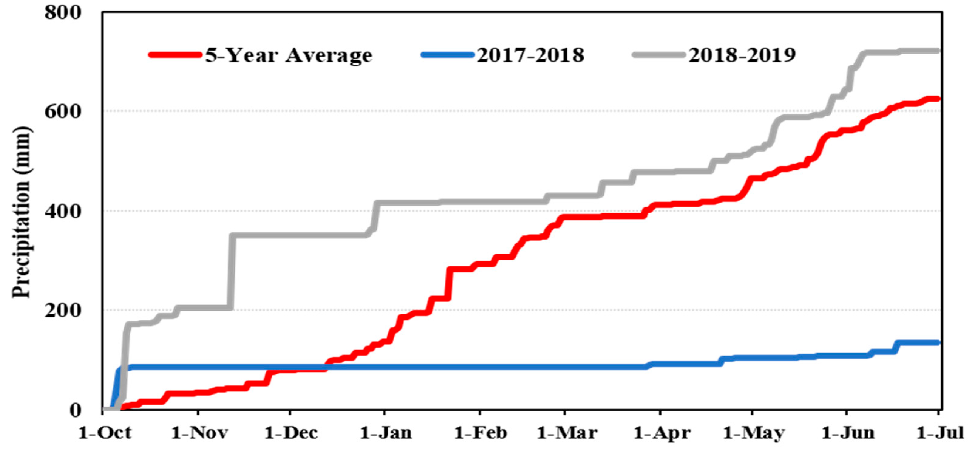
2.1. Study Area

Field experiments were conducted at the Texas A&M AgriLife Research Experiment Station at Bushland, Texas (35°11′ N, 102°06′ W, elevation 1170 m) in 2017–2018 (2018) and 2018–2019 (2019) winter wheat growing seasons (Figure 1). 21 genotypes were grown in 2018 and 22 were grown in 2019 under irrigated and dryland water regimes. The genotypes comprised released varieties and advanced lines from the Uniform Variety Trial (UVT) of Texas A&M’s wheat breeding program. The experimental design was a randomized complete block design with three replications. Plots were 4.5 m × 1.5 m in size under the irrigated condition and 6.1 m × 1.5 m under dryland condition, consisting of seven rows with 0.18 m spacing. Seeds were sown on October 11 (dryland) and October 17 (irrigated) in 2017 and on October 30 (dryland) and November 15 (irrigated) in 2018 (Table 1). Agronomic practices such as nutrient and weed management were conducted when needed following the regional practices. The irrigated field received 343 mm and 95 mm irrigation in 2018 and 2019, respectively. Irrigation was applied with a three-span, lateral-move sprinkler system (Model 6000, Valmont Irrigation, Valley, NE, USA). The 2018 season was extremely dry and relatively hot compared to 2019 (Figure 2 and Figure 3). Growing season precipitation in 2019 was 700 mm and 150 mm in 2018 (40 percentage of climate normal: calculated using the data from www.ncdc.noaa.gov, accessed on 1 January 2021).

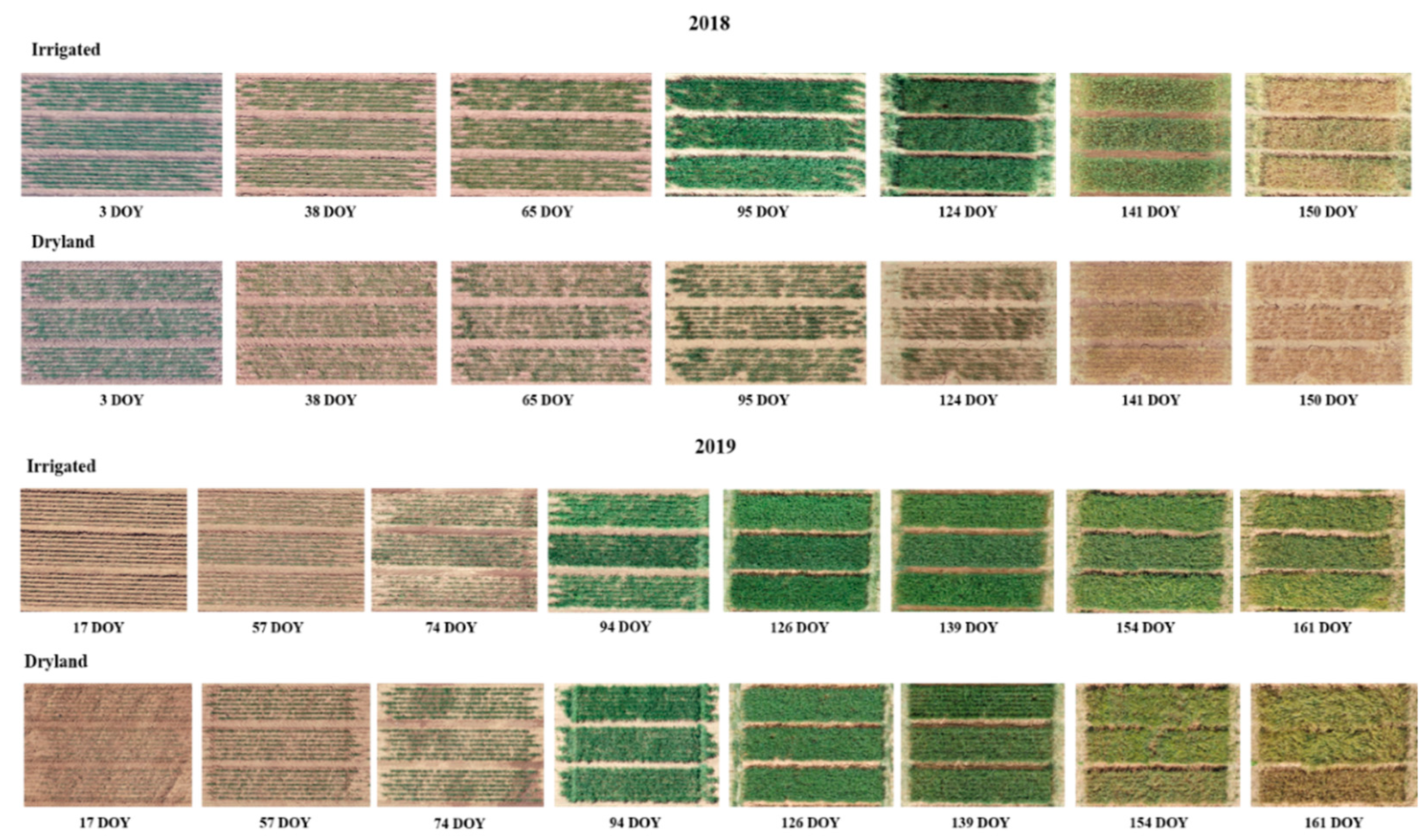
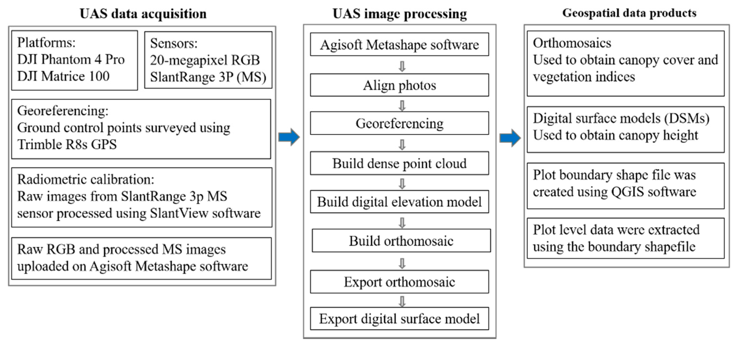
2.2. UAS Data Collection

We obtained multispectral (MS) images by flying a DJI Matrice 100 quadcopter (SZ DJI Technology Co., Ltd., Shenzhen, China) equipped with an MS sensor: SlantRange 3P (SlantRange, Inc., San Diego, CA, USA). The SlantRange 3p has four 1.2-megapixel resolution sensors with central wavelengths of 550 nm (green), 650 nm (red), 720 nm (red-edge), and 850 nm (NIR). The spectral range covered by the green, red, red-edge, and NIR bands were 545–555 nm, 640–660 nm, 710–720 nm, and 840–860 nm, respectively. The SlantRange 3P sensor has a global shutter, and it has an onboard ambient illumination sensor that can be used to perform radiometric calibration in the post-processing stage. Therefore, data captured by the SlantRange 3P sensor throughout a single flight and from flight-to-flight during the growing season are comparable and consistent concerning changing weather conditions. Another platform, DJI Phantom 4 Pro equipped with a red, green, blue (RGB) sensor (SZ DJI Technology Co., Ltd., Shenzhen, China), was flown to collect RGB images. Phantom 4 Pro was flown at 15–20 m with 80–85% forward and side overlap to obtain 0.3–0.5 cm/pixel GSD (Ground Sampling Distance) when processed to generate orthomosaic images. Matrice 100 was flown at 30–35 m with a 70–75% overlap to get 1.2–1.7 cm/pixel GSD when processed to generate orthomosaic images. Nine semi-permanent ground control points (GCPs) were placed across the field after planting, and precise coordinates of the GCPs were surveyed using Trimble R8s Global Positioning System (GPS) (Trimble Inc., Sunnyvale, CA, USA). Coordinates of the GCPs were used in the structure from motion (SfM) process to ensure accurate georeferencing of the UAS-based geospatial data products. Data were collected at 7 to 15 days intervals throughout the growing season (Figure 4).

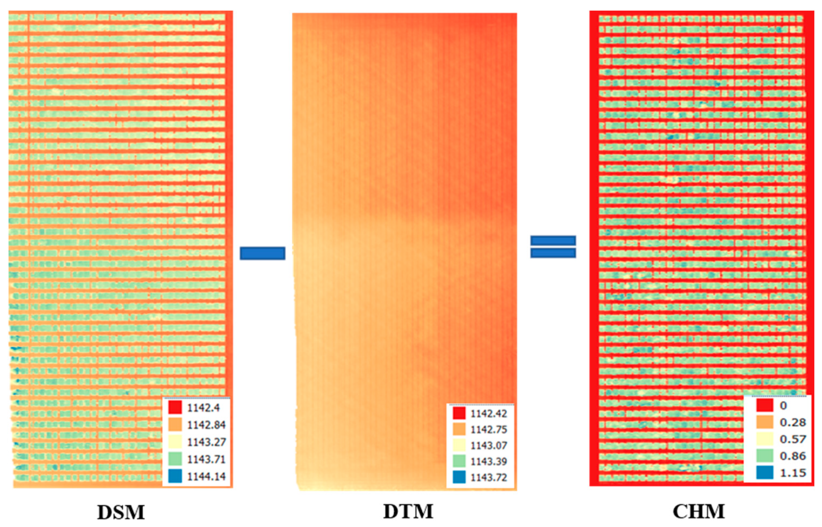
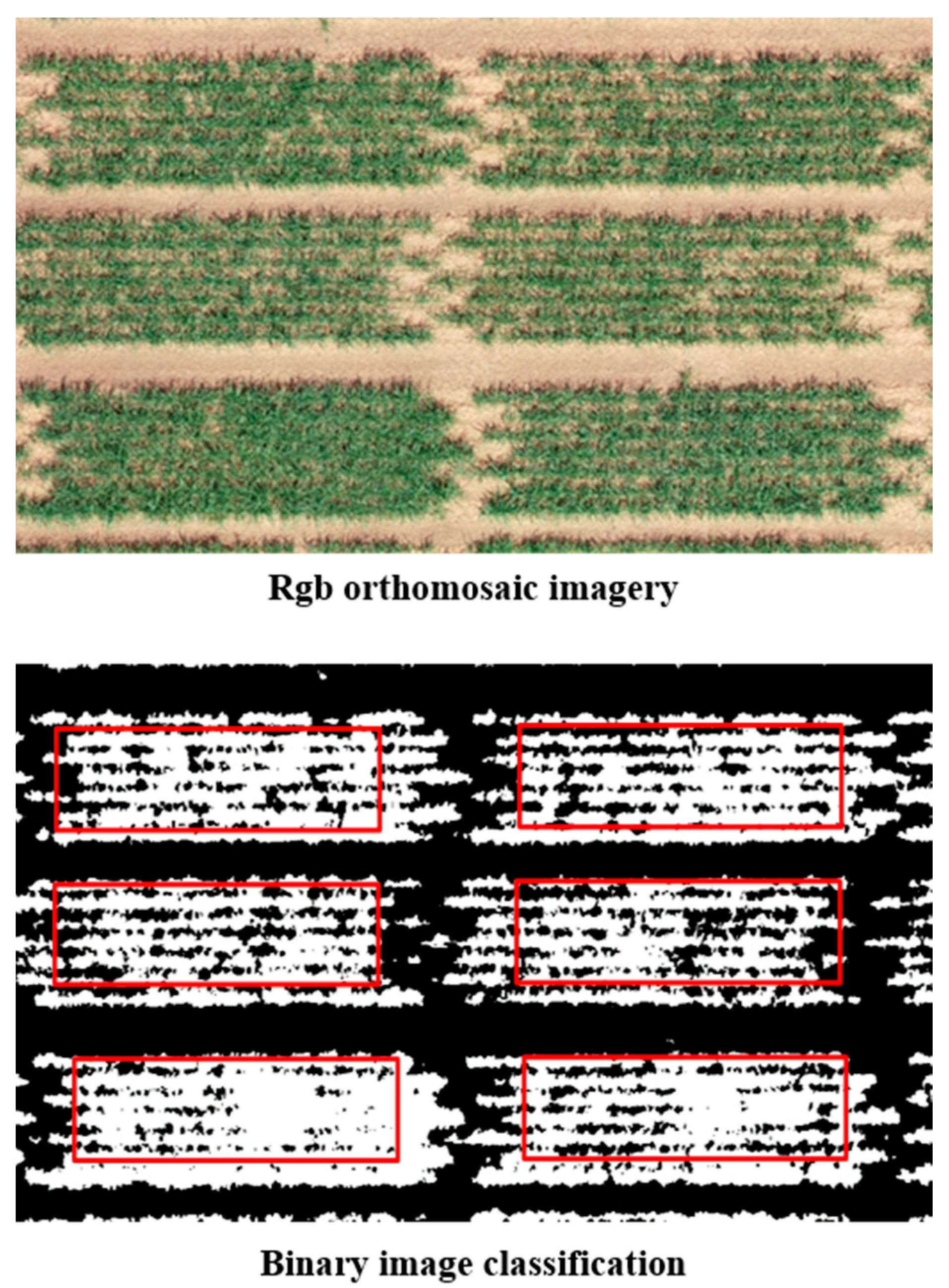
2.3. UAS Data Processing

Raw images obtained from the MS sensor were first processed using SlantView software (SlantRange, Inc., San Diego, CA, USA) to acquire radiometrically calibrated MS images. These images, along with raw RGB images, were processed using Agisoft metashape software (Agisoft LLC, St. Petersburg, Russia, 191144) to generate geospatial data products such as a 3D point cloud, Digital Surface Model (DSM), and orthomosaic images (Figure 5). CC, ExG, NDVI, and NDRE were computed from orthomosaic images. Digital Terrain Model (DTM) of bare ground surface was generated from the images obtained after planning. Canopy Height Model (CHM) was obtained by subtracting DTM from DSM generated after every flight during the crop growth (Figure 6). A plot boundary polygon layer was overlaid on CHM and measurement in 95th percentile height value within each polygon was extracted as the representative canopy height for each plot.
CC was obtained by applying the Canopeo algorithm developed by Patrignani and Ochsner [42] to the RGB orthomosaics. In this approach, a certain threshold was used to classify the image into the canopy and non-canopy classes, and a binary image was produced by applying equation 1 during image processing.
R G < P 1   ,         B G < P 2   ,             2 G R B > P 3
where R, G, and B are Digital Number (DN) values for the red, green, and blue bands, respectively. P1 and P2 are parameters to classify pixels in the green band and P3 sets the minimum value for ExG (Table 2) to select green vegetation. In this study, parameter (P1, P2, and P3) values were set to default as explained in the Canopeo algorithm (P1 = 0.95, P2 = 0.95, and P3 = 20) [42]. A plot boundary polygon layer was overlaid on the classified image and the percentage of canopy cover was calculated using Equation (2) (Figure 7).
Canopy   Cover   ( CC ) = Total   number   of   canopy   pixels Total   number   of   pixels × 100
Three VIs were obtained, of which two indices, NDVI and NDRE, were obtained from the MS sensor, whereas ExG was obtained from the RGB sensor (Table 2). A plot boundary polygon layer was overlaid on the VIs map and the plot average value was extracted.
Table 2. List of spectral vegetation indices. Reflectance obtained in red, green, blue, red-edge, and near-infrared region of the spectrum is denoted by R, G, B, RE, and NIR, respectively.
Vegetation IndicesFormulaReferences
Excess Green Index (ExG) E x G = 2 G R B [42]
Normalized Difference Red-edge Index (NDRE) N I R R E N I R + R E [43]
Normalized Difference Vegetation Index (NDVI) N I R R N I R + R [44]

2.4. Ground Measurements

Manual plant height measurements were collected before harvest. A single measurement was taken per plot from the base of the plant to the tip of the spike. The heading date was recorded when 50% of spikes in a plot were fully exposed. In 2018, genotypes reached the heading date at 113–123 DOY and 119–127 DOY in the dryland and irrigated environments, respectively. Heading was much earlier than normal in 2018 due to drought stress. In 2019, it was in line with the long-term average; 122–129 DOY in dryland and 124–135 DOY in the irrigated environment. Each plot was harvested using a small plot combine (Classic Plus, Wintersteiger AG, Germany) to determine the final grain yield.

2.5. Data Analysis

Obtained UAS measurements were averaged across plots for each measurement date to compare the seasonal dynamics of canopy traits between the dryland and irrigated environment. Obtained measurements were plotted against the day of the year (DOY) to develop graphs for seasonal trends. DOY is the number representing the day between 1 and 365 of a year (DOY of January 1 is 1). Standard deviation was calculated across environments to show the variation in the UAS measurements. Data analysis was conducted using SAS version 9.4 (Statistical Analysis System Institute, Cary, NC, USA). PROC CORR procedure in SAS was used to determine Pearson correlation coefficients (r) between grain yield and UAS-based canopy traits. The coefficient of determination (R2) was calculated to assess the relationship between ground-based plant height and UAS-based canopy height measurements.

3. Results

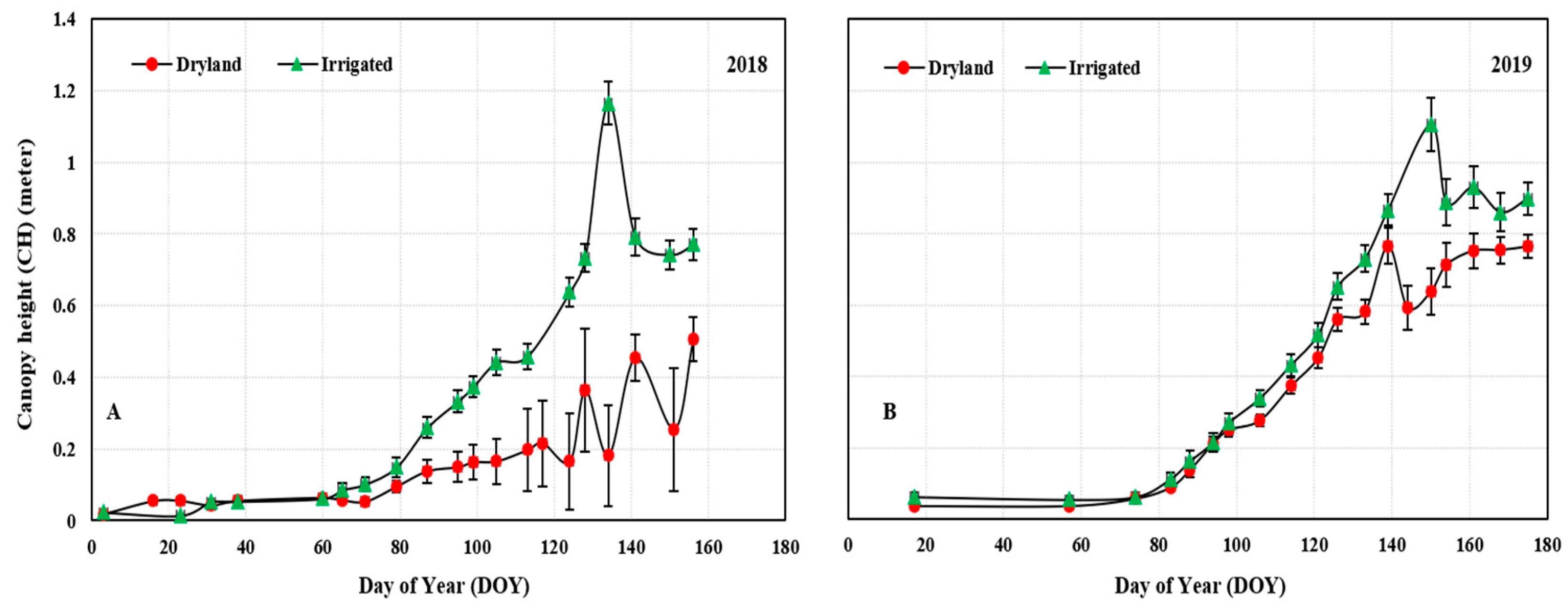
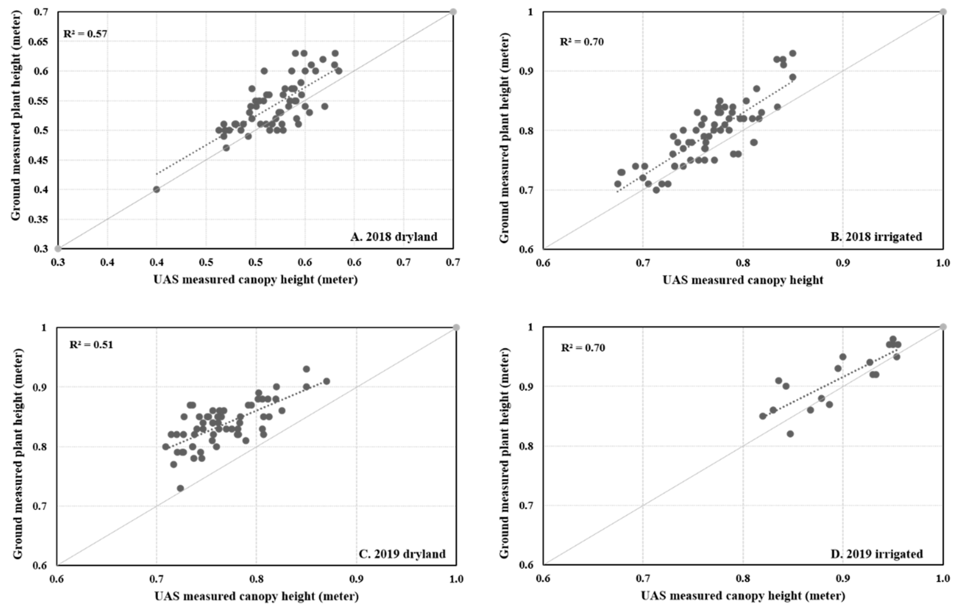
3.1. Temporal Dynamics of CH

In general, CH began to increase from the first week of March (60 DOY) in 2018 (Figure 8A) and the second week of March in 2019 (74 DOY) (Figure 8B) with the increase in air temperature. Dryland CH was relatively low in both years once the growth started. The difference in CH between the two water levels was highly significant throughout the season in 2018. Extreme drought in 2018 resulted in reduced growth and the plants did not grow much more than 0.5 m tall. However, under irrigation, CH increase was linear and reached a maximum of 1.2 m by the second week of May (134 DOY). In 2019, under both environments, CH followed a similar trend as in the 2018 irrigated environment. CH reached maximum 10 days earlier (140 DOY) in dryland compared to irrigated environment (150 DOY). Average CH was 1.1 m and 0.75 m in irrigated and dryland environments, respectively (Figure 8B). Significant differences in CH measurements between irrigated and dryland environments were observed after this point. CH measurements in the dryland environments were low in both years compared to the irrigated environments. In general, there was a sudden decline in CH after reaching the plateau except in 2018 dryland where the plants dried down early amid severe drought stress.
CH measured from UAS were validated with ground-based manual measurements (Figure 9). A linear relationship was found between UAS-obtained CH measurements and ground-based measurements. The R2 values ranged from 0.5 to 0.7 depending on the environment. Hassan et al. [36] found a strong correlation (R2 = 0.8–0.9) between UAS and ground-based plant height data measured at the booting and mid-grainfilling stages. Relationships were relatively strong under irrigated condition in both years compared to the dryland. Lower correlations are due to the time at which manual measurements were taken. Manual measurements were taken from a single plant per plot after crop maturity when there are high chances of lodging and disturbance in the canopy structure. Underestimation of CH by UAS as seen in some previous studies [45] was found in our study across all environments. Considering the seasonal trend of CH and accuracy of data validation, UAS can be an important alternative tool to obtain CH measurements of wheat research plots.

3.2. Temporal Dynamics of CC

In 2018 canopy growth started early in the season (Figure 10A). The CC was already 40–50% in the first week of January and remained in the same range until the end of January (31 DOY). Low temperature caused a dip in CC values in the first week of February (38 DOY). CC values gradually increased after reduced winter growth in both environments and reached 90–100% in the irrigated environment and 45–55% in the dryland. Canopy growth started late in 2019 (Figure 10B). CC was less than 5% until the last week of February (57 DOY) when it started to grow rapidly and reached a maximum of 100% and 88 % in the first week of April (98 DOY) under irrigated and dryland environments, respectively. CC remained the same until the third week of May (139 DOY) and started to decrease gradually and reached 1% in the first week of June (168 DOY) under irrigation. In the dryland environment, the reduction in CC values started a week earlier (133 DOY) and reached 1% by 161 DOY. CC measurements clearly depicted the environmental conditions. In the severe drought year of 2018, peak CC measured in the irrigated environment was double that measured in the dryland environment. Significant differences in CC were also found in 2019, but the difference was considerably less than in 2018. Canopy growth followed a sigmoidal growth function in 2019 with slow early growth in the beginning followed by a linear growth phase, and then a steady stage. The decline in CC after the steady stage is attributed to senescence. The changes in the color of the canopy across different environments are shown in Figure 4. The trend of CC aligns well with the seasonal change in ground cover and reached maximum when the ground was fully covered by the canopy. This shows the usefulness of estimating CC using UAS to calculate ground cover and assess the effect of drought on vegetation growth.

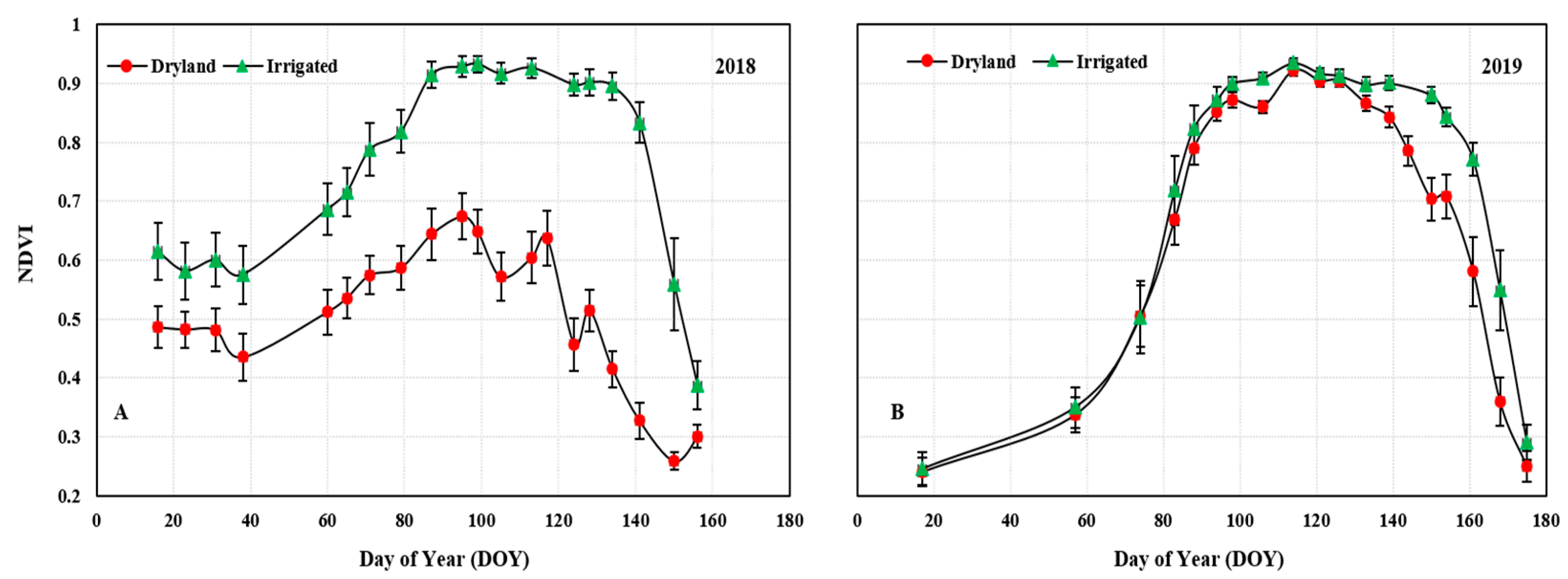
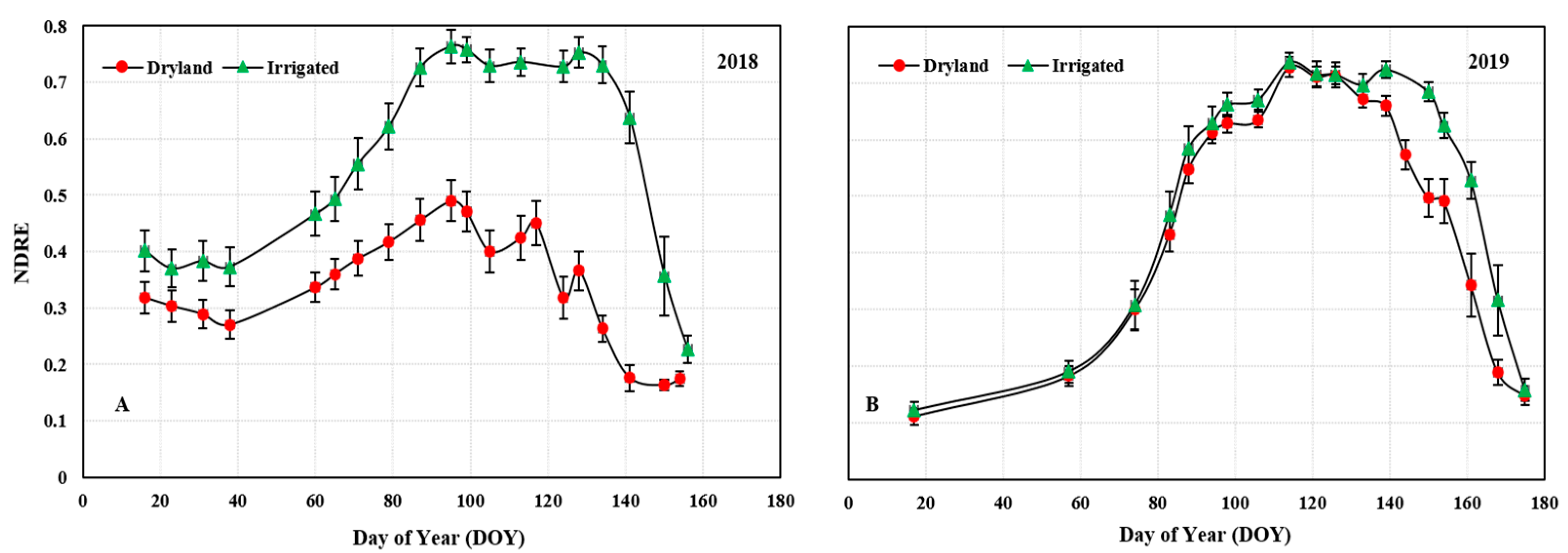
3.3. Temporal Dynamics of VIs

The temporal dynamics of NDVI, NDRE, and ExG obtained from UAS during the wheat growing season is shown in Figure 11, Figure 12, and Figure 13, respectively. General growth pattern of these indices was similar to CC across all the environments. The pattern can be divided into four stages based on the greenness of the canopy; germination and stand establishment, accelerated vegetative growth accompanied by tillering, steady stage when the ground was fully covered by the canopy, and a declining stage during physiological maturity.
NDVI was obtained from MS sensor and uses the visible and NIR light. This index has been widely used to monitor vegetation dynamics and crop health. Drought significantly affected NDVI measurements in our study. The effect was proportionate to the intensity of drought as seasonal NDVI values were low in dryland condition compared to irrigated condition in 2018 (Figure 11A). As the experimental site received frequent precipitation in 2019, dryland NDVI measurements were similar to irrigated measurements (Figure 11B) until heading (135 DOY). The difference was significant once the heading was completed, and plants began to senescence. The decline in NDVI during senescence was slow under irrigated condition compared to dryland. The seasonal trend of NDVI was relatively smooth in 2019 compared to 2018 in the dryland environment with minimum lows and highs. NDVI values ranged from 0.2 to 0.7 in the dryland and 0.4 to 0.9 in the irrigated environment in 2018. Values were higher in 2019 and ranged from 0.2 to 0.95 in both dryland and irrigated environments.
NDRE was also calculated from radiometrically calibrated MS orthomosaics. It uses the NIR and red-edge light which is the transition region between the visual red and NIR light. NDVI is prone to early saturation in dense vegetation [46] and NDRE can serve as an alternative to NDVI to assess spatial and temporal variabilities [47,48]. In our study, both NDVI and NDRE curves closely resemble each other. NDRE values ranged from 0.1 to 0.8 in all environments except in 2018 dryland in which the values ranged from 0.1 to 0.5. The effect of drought was severe in 2018 compared to 2019 as NDRE measurements were relatively low throughout the growing season (Figure 12A). Dryland and irrigated NDRE measurements were about the same in 2019 and differences were not significant until after heading (135 DOY) (Figure 12B).
ExG was calculated utilizing the broad band lights from RGB sensor. Compared to MS-based indices, the trends were similar with early slow increase followed by linear growth, and decline at later growth stage, but there were higher oscillations across all environments (Figure 13). In 2018, under irrigated conditions, ExG reached a maximum at 99 DOY and had a dip on 105 and 113 DOY (Figure 13A). It again reached a plateau on 124 DOY and then started to decline. The dryland ExG never exceeded 0.1 in the dryland. In 2019, ExG values ranged from 0.1 to 0.45 in irrigated condition and the values in dryland ranged from 0.1 to 0.35. The drop in ExG values were highly proportionate to the intensity of drought. In 2019, ExG values increased consistently but after attaining the plateau inconsistent patterns were noted. In some DOYs, values were high while in others there were dips (Figure 13B). The fluctuations happened when CC, NDVI, and NDRE remained steady during the 90–100% ground cover. ExG was highly sensitive to weather variations and change in the color of the canopy (Figure 4).

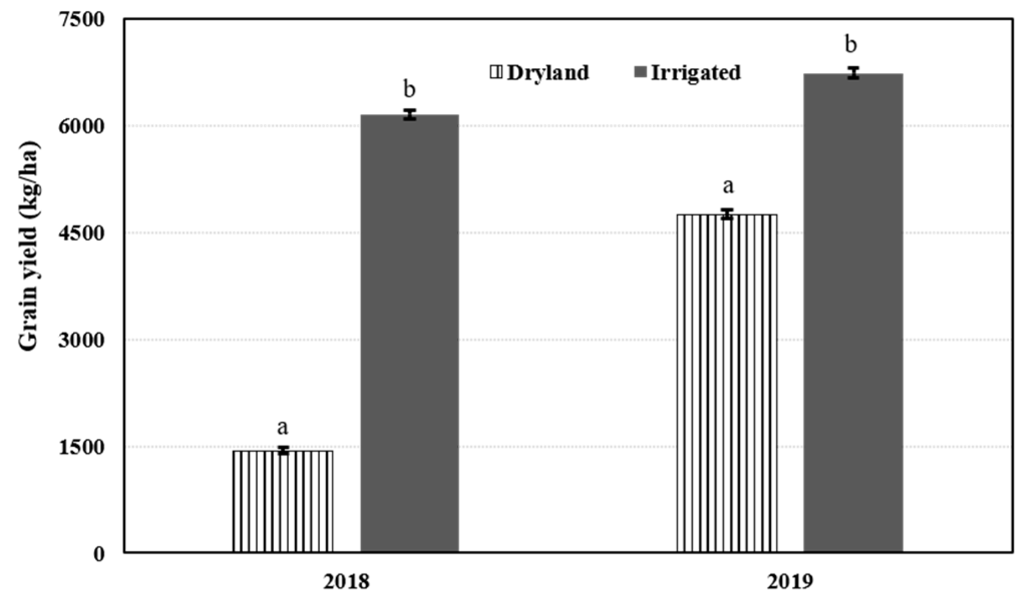
3.4. Correlations Between Grain Yield and UAS-Based Parameters

There was a significant (p < 0.05) difference in grain yield between dryland and irrigated environments in both years. The Yield gap between the two environments was much higher in 2018 compared to 2019 which is the result of low precipitation 2018. Mean dryland yield was 1500 kg ha−1 and 4755 kg ha−1 in 2018 and 2019, respectively (Figure 14). Under the irrigated conditions, the yield was 6156 kg ha−1 and 6738 kg ha−1 in 2018 and 2019, respectively.
In general, the correlation of grain yield with the UAS-based canopy traits obtained early in the growing season was weak compared to traits obtained after heading through maturity (Table 3). In 2018 dryland, CC, CH, and EXG had lower correlation coefficients (r) compared to NDRE and NDVI most of the times during the growing season. Significant (p < 0.05) r values greater than 0.3 for CC and ExG were on 87–97 DOY (boot stage) and 117–128 DOY (heading, anthesis and grain filling). Similarly, CH had r values greater than 0.3 during 117 DOY. NDRE and NDVI had r significant and greater than 0.3 during 99 DOY to 134 DOY (boot, heading, anthesis, and grain filling stage). The highest r value found in this environment was 0.58 (p < 0.05) from NDRE during grain filling period. CC, CH, and ExG were obtained from RGB images while NDVI and NDRE were obtained from radiometrically calibrated MS images. Plots in 2018 had early ground cover compared to 2019 (Figure 10A) but this early biomass accumulation was not related to final grain yield. Lack of seasonal precipitation along with the reduction of available soil water during heading, anthesis, and grain filling might be the reason for not having higher correlation between yield and UAS-based canopy features measured early in the season. The 2018 irrigated environment was better with higher r values of canopy traits with grain yield. CC and ExG performed better than NDRE and NDVI with higher r values. CC had r values greater than 0.3 most of the times except 23–38 DOY (early tillering stage) and 99 DOY. CH had higher r values at 134–150 DOY (after heading). Higher r values of ExG (r > 0.45, p < 0.05) was during 105 DOY to 150 DOY (pre-heading, heading, anthesis, and grain filling stage). NDRE and NDVI also had higher r values multiple times during the growing season. The highest r value found in 2018 irrigated environment was 0.57 (p < 0.05) from ExG measured during the grain filling period (134 DOY).
The 2019 dryland environment was favored by frequent rainfall events. Additionally, early season canopy coverage was low compared to 2018. CC, CH, ExG, NDRE, and NDVI measured until 126 DOY had non-significant correlation (p > 0.05) with yield (Table 3). However, r values improved following heading. Anthesis and grain filling stages had higher r values for all the traits (r > 0.4, p < 0.05). CC measured at 144 DOY under dryland environment in 2019 had the highest correlation coefficient (r = 0.71, p < 0.05) among all the environments. Effect of water stress was not visible in the canopy as in 2018. All the plots achieved 90 percent ground cover during 100–133 DOY (Figure 10B) under 2019 dryland environment. The higher correlation of CC, ExG, NDVI and NDRE might be related with the rate of senescence and stay green ability of genotypes during grain filling period. The 2019 irrigated season showed a different phenomenon regarding the correlation between VIs and grain yield. Except CH, correlation was either negative (r = 0.14–0.40) or non-significant (p > 0.05). ExG had highest r values in 2018 irrigated condition but in 2019 the correlation was negative. A similar pattern was shown by CC, NDRE, and NDVI. Plots attained maximum ground cover in 94 DOY and maintained 100 percent canopy coverage until 144 DOY. Senescence in 2019 started late and was slower than in 2018. The variability among the plots was low with respect to change in canopy cover which might have contributed to lower correlation values in the 2019 irrigated environment. CH measured at 121–133 DOY, however, had better r values (r > 0.3, p < 0.05).

4. Discussion

4.1. Growth Dynamics based on UAS-Based Canopy Traits

All the canopy traits: CC, NDVI, NDRE, and ExG, followed general growth characteristics of winter wheat. These traits started with slow growth at the beginning of the season (germination and early stand establishment), and as the season progressed (tillering), showed linear growth (stem elongation along with canopy growth), and reached a plateau of maximum ground cover. The plateau lasted until heading which was again followed by a slow decline until maturity. The decrease in VIs and CC after heading is attributed to the change in color of the canopy because of senescence and physiological maturity [49]. A similar growth pattern of canopy attributes and vegetation indices was observed in other studies [36,50,51,52,53,54]. Although the growth trend was similar to these studies, the time of event differed in our study. For example, Lin et al. [55] recorded highest NDVI value during the heading stage of wheat but maximum CC, NDVI, and NDRE were achieved 10–15 days before heading in our study. This was mainly because high tillering and increased vegetation growth led to early canopy saturation. Similar results were observed by Song and Wang [56] in a phenology study conducted using Sentinel-1 data. In the case of plant height, except for the 2018 dryland, CH followed a sigmoidal growth pattern and reached maximum during heading followed by slight reduction once it reached its maximum. Anderson et al. [57] also found a similar trend in seasonal plant height measured by UAS in maize. There was some lodging in our study which reduced the average value in the late growing season. Although the nature of the trend was similar in 2018 and 2019, some canopy traits exhibited difference in the time and duration of phenological changes. For example, all the traits showed higher values between 0 to 40 DOY in 2018 compared to same period in 2019 which was due to early planting in 2018 complemented by moisture stored in the soil due to precipitation before planting in 2017.
Combining the seasonal trend of CC and CH obtained in our study might be useful to assess the phenology of winter wheat growth. The growth dynamics can be divided into four different stages by looking at the CC and CH curves. Slow early growth with an increase in ground cover during the tillering stage, the onset and duration of linear growth can be classified as stem elongation period. The point at which CH reached maximum and CC starts to decline (150 DOY) happened after heading and at the onset of flowering. The duration of the decline in CC can be classified as a ripening stage. Slow early growth can be used to assess early stand establishment and vigor [58]. Linear growth in CH and CC can be used to assess maximum canopy growth and duration to achieve and maintain maximum ground cover. The decline of CC can be used to assess senescence rate [50,52], and stay green [59,60] phenotypes. Another approach to differentiate phenological stages is by using VIs. Magney et al. [61] used spectral reflectance radiometers to collect daily NDVI measurements to monitor crop phenology of soft white spring wheat. Four phenological growth stages namely, tillering, stem elongation, heading, and ripening were derived by fitting a non-parametric regression curve on the daily measurements. Zheng et al. [62] used first order derivative of time series NDVI measurements to estimate the time of tillering, heading, and maturity in rice. Chu et al. [55] used MODIS time series data and fitted double Gaussian function to detect green-up, heading, and harvesting phases of wheat. Successful detection of phenological phases can be beneficial to wheat breeders to screen genotypes for respective traits. Early detection of these phases can be helpful to assess the future drought impact on canopy growth and can support farmers to make management decisions. Although it needs further research and validation, this study showed the possibility of using multi-temporal UAS data collected over the entire season to estimate the time of phenological phases in winter wheat.
Several physiological and biochemical traits [63,64,65,66,67] have been evaluated and proposed to screen genotypes for drought tolerance in wheat. However, in traditional breeding programs grain yield is the primary trait used to make selection decisions [68]. The spatial and temporal constraints of measuring physiological traits in many genotypes limits their use in plant breeding. Methodologies used in this study can be useful to obtain data of yield-associated traits that can be used to identify genotypes that can resist, tolerate, or adapt under water-limited conditions. The ability to track the seasonal dynamics of these traits can help to understand the time, intensity, and duration of the impact of drought on canopy growth. Additionally, integration of different traits can help to dissect the effect of drought according to key phenological stages [67]. For example, CC can be used to estimate early ground cover and NDRE can be used to estimate senescence rate and calculate stay-green duration, thus optimizing the utilization of available soil water [68].
MS sensor-based indices were more stable than ExG (obtained from RGB sensor). Weekly ExG measurements had a higher standard deviation on individual dates and were more sensitive to the changes in canopy color and weather conditions. A notable difference was seen during low winter temperatures and recovery in CC (60–60 DOY, Figure 10A). Radiometric calibration of the MS sensor can be attributed to its stable measurements [69] compared to the RGB sensor.
Drought significantly affected canopy growth. Differences in the growth curves of UAS-based canopy traits between the dryland and irrigated condition clearly illustrated the impact of drought on canopy growth, which other studies also found [36,70,71,72]. Dryland CC values in 2018 started off strong but lagged as the season progressed due to the extreme drought in 2018. In 2019, the increase in CC started once irrigation was applied and CC in the irrigated environment remained higher throughout the season. The difference between dryland and irrigated environment was larger after heading which is indicative of moisture stress during the reproductive stage [60] as dryland plants could not maintain greenness. Drought significantly reduces leaf water potential, relative leaf water content [41], chlorophyll content [73], stomatal conductance, and photosynthesis [74] resulting in canopy wilting, stunted growth, and leaf area reduction [41]. Positive correlations exist between VIs and physiological traits such as leaf equivalent water thickness, canopy water content (CWC) [75] and chlorophyll content [76]. The difference in UAS derived canopy traits between dryland and the irrigated environment was clearly reflected in respective yield differences in both years. Thus, the seasonal patterns of UAS-based canopy features can enhance our understanding of the effect of drought and crop management practices on vegetation growth [77].

4.2. Association between UAS-Based Canopy Traits and Grain Yield

A consistent positive correlation between UAS-based canopy traits and grain yield was found under the dryland environment in both years. The relationship between spectral VIs and grain yield under dryland has been established in several previous studies [78,79,80,81]. Canopy features and vegetation indices determined by the amount and intensity of the green canopy has been used to estimate above-ground biomass in wheat [82,83,84] and the biomass is correlated with grain yield [85]. This leads to the association of canopy features with grain yield. Naser et al. [49] found a positive association between wheat grain yield and NDVI measured at anthesis, and during grain filling period under dryland environment. Thapa et al. [85] also found a significant correlation between yield and NDVI measured after the jointing stage of wheat. However, they cautioned about using NDVI for screening genotypes for yield under extreme drought conditions. Our 2018 dryland environment went through extreme drought with less than 150 mm precipitation during the entire growing season. Even with the extreme drought in 2018, a significant positive correlation was observed between yield and UAS-based canopy features measured during anthesis to maturity. Our results showed that VIs generated from MS sensor yielded higher correlation coefficients compared to ones obtained from the RGB sensor. In contrast to the 2018 experiment, 2019 was moderate in drought, and the correlation between grain yield and UAS-based features improved significantly.
A significant positive relationship between yield and each of CC and VIs was found in the 2018-irrigated environment. Like dryland environment, the UAS-based features obtained after heading had stronger correlations with grain yield. This result agrees with Thapa et al. [85] in which they showed a positive relationship between yield and Green Seeker-based NDVI data obtained in the same location using different sets of genotypes in the same year. Positive correlation between spectral indices and grain yield under irrigated environment was found in several other studies in wheat [36]. However, in 2019, the nature of this correlation was different. Except for CH, the relationships were either non-significant or negative. Genotypes in 2019 were not water-stressed as the available water was higher than normally required during the growing season. Early canopy saturation reduced the variability in UAS-based canopy features within the irrigated environment as plants attained maximum canopy size and maintained greenness which might be the reason for not obtaining a similar correlation trend as in other environments. The uniformity in the greenness of the canopy might be the reason for reduced ability of the canopy traits to differentiate genotypes with respect to yield. Naser et al. [49] also found a poor association of NDVI with wheat grain yield in irrigated environments and suggested that NDVI can perform a better job when the sensor is not saturated. The results obtained by Casadesus et al. [78] also support the findings of our study as the NDVI measured during anthesis of wheat genotypes was not able to provide better yield estimation because of complete soil coverage and high plant density. Four irrigation events on 66, 98, 107, and 136 DOY, along with higher precipitation, caused higher vegetative growth and excessive biomass accumulation in our study. It can be inferred that the CC and VIs used in this study are not effective to estimate yield in winter wheat with excessive biomass.
Finding optimal time for collecting UAS data to assess drought tolerance with respect to yield is important to plant breeders to reduce the cost of data collection and processing. In our study, we collected UAS data on a weekly basis, almost 20 times during the season. Even in a moderate drought year like 2019, RGB data collected after 100 DOY and MS data collected after 130 DOY were valuable to find the impact of drought in the canopy. Additionally, the yield was highly correlated with UAS-based canopy features measured after heading as in other studies. Hassan et al. [36] found lower correlation coefficients of yield with VIs measured during early growth stages like stem elongation, booting, and heading. Selecting cultivars based on the measurements obtained after heading especially, during anthesis and grain filling period [49,85,86], seem efficient, but our results suggest that taking multiple measurements across several growth stages can add significant benefits to the screening process.

5. Conclusions

This study demonstrated the collection, processing, and phenotypic feature extraction procedure of UAS. Experimental results showed that the multi-temporal UAS data is useful for monitoring winter wheat growth and assessing the impact of drought on canopy growth. UAS-based canopy traits were affected by the intensity of drought on wheat vegetation. Besides, the integration of season-long multi-temporal canopy features and vegetation indices showed the potential to identify the phenological growth stages and assess the impact of drought at these different stages. Traits obtained from the MS sensor were more stable than from the RGB sensor since radiometric calibration improved the stability of measurements across time. UAS-based traits obtained from heading to maturity correlated with grain yield. However, the relationship largely depends on the growing conditions and may not always predict yield, especially when the canopies are dense. Multi-temporal UAS-based canopy traits can be used to capture the response of various physiological attributes that cumulatively affect yield under drought. Integration of UAS-based remote sensing, agronomy, wheat breeding, and data analytics can potentially develop digital tools that can be used to select genotypes for drought tolerance and improve the genetic gain of wheat breeding programs.

Author Contributions

Conceptualization, M.B., A.M.H.I. and J.C.R.; methodology, M.B., Q.X., A.C., J.J. and J.L.; software, A.C. and J.J.; formal analysis, M.B.; resources, B.A., J.C.R., A.M.H.I., S.B.; data curation, S.B.; writing—original draft preparation, M.B., Q.X., A.M.H.I.; writing—review and editing, M.B., A.M.H.I., Q.X., J.C.R., J.J., S.B. and A.C.; funding acquisition, A.M.H.I., Q.X., J.C.R. All authors have read and agreed to the published version of the manuscript.

Funding

This research received no external funding.

Institutional Review Board Statement

Not applicable.

Informed Consent Statement

Not applicable.

Data Availability Statement

The data presented in this study are available on request from the corresponding author. The data are not publicly available due to privacy.

Acknowledgments

Authors would like to acknowledge Texas A&M AgriLife Crop Improvement Initiative, Texas A&M AgriLife Research Cropping System Program, Texas Wheat Producers Board, and USDA-NIFA Hatch Project TEX09438 for their financial support in this project.

Conflicts of Interest

The authors declare no conflict of interest.

Abbreviations

CCCanopy Cover
CHMCanopy Height Model
CHCanopy height
DEMDigital Elevation Model
DSMDigital Surface Model
DTMDigital Terrain Model
ExGExcess Green Index
GPSGlobal Positioning System
GSDGround Sampling Distance
HTPHigh-Throughput Phenotyping
MSMultispectral
NIRNear-InfraRed
NDRENormalized Difference Red-edge Index
NDVINormalized Difference Vegetation Index
UVTUniform Variety Trial
UASUnmanned Aerial System
VisVegetation indices

References

  1. Plains, S.; Field, R.; Post, O.; Box, O. May Crop Production Texas Wheat Production and Yield. 2020; 9992, 2019–2020. Available online: https://www.nass.usda.gov/Statistics_by_State/Texas/Publications/Current_News_Release/2020_Rls/spr-crop-prod-05-2020.pdf (accessed on 1 January 2021).
  2. Ray, R.L.; Fares, A.; Risch, E. Effects of Drought on Crop Production and Cropping Areas in Texas. Agric. Environ. Lett. 2018, 3, 170037. [Google Scholar] [CrossRef] [Green Version]
  3. Anderson, D.P.; Welch, J.M.; Robinson, J. Agricultural Impacts of Texas’s Driest Year on Record. Choices AAEA 2012, 27, 1–4. [Google Scholar]
  4. Bacelar, E.L.V.A.; Moutinho-Pereira, J.M.; Gonçalves, B.M.C.; Brito, C.V.Q.; Gomes-Laranjo, J.; Ferreira, H.M.F.; Correia, C.M. Water Use Strategies of Plants under Drought Conditions. In Plant Responses to Drought Stress: From Morphological to Molecular Features; Springer: Berlin/Heidelberg, Germany, 2012; pp. 145–170. [Google Scholar] [CrossRef] [Green Version]
  5. Nezhadahmadi, A.; Prodhan, Z.H.; Faruq, G. Drought Tolerance in Wheat. Sci. World J. 2013. [Google Scholar] [CrossRef] [Green Version]
  6. Blum, A.; Pnuel, Y. Physiological Attributes Associated with Drought Resistance of Wheat Cultivars in a Mediterranean Environment. Aust. J. Agric. Res. 1990, 41, 799–810. [Google Scholar] [CrossRef]
  7. Sallam, A.; Alqudah, A.M.; Dawood, M.F.A.; Baenziger, P.S.; Börner, A. Drought Stress Tolerance in Wheat and Barley: Advances in Physiology, Breeding and Genetics Research. Int. J. Mol. Sci. 2019, 20, 3137. [Google Scholar] [CrossRef] [Green Version]
  8. Rashid, A.; Stark, J.C.; Tanveer, A.; Mustafa, T. Use of Canopy Temperature Measurements as a Screening Tool for Drought Tool for Drought Tolerance in Spring Wheat. J. Agron. Crop Sci. 1999, 231–238. [Google Scholar] [CrossRef]
  9. Deery, D.M.; Rebetzke, G.J.; Jimenez-Berni, J.A.; James, R.A.; Condon, A.G.; Bovill, W.D.; Hutchinson, P.; Scarrow, J.; Davy, R.; Furbank, R.T. Methodology for High-Throughput Field Phenotyping of Canopy Temperature Using Airborne Thermography. Front. Plant Sci. 2016, 7. [Google Scholar] [CrossRef] [PubMed] [Green Version]
  10. Kamal, N.M.; Gorafi, Y.S.A.; Abdelrahman, M.; Abdellatef, E.; Tsujimoto, H. Stay-Green Trait: A Prospective Approach for Yield Potential, and Drought and Heat Stress Adaptation in Globally Important Cereals. Int. J. Mol. Sci. 2019, 20, 5837. [Google Scholar] [CrossRef] [Green Version]
  11. Manschadi, A.M.; Christopher, J.; Devoil, P.; Hammer, G.L. The Role of Root Architectural Traits in Adaptation of Wheat to Water-Limited Environments. Funct. Plant Biol. 2006, 33, 823–837. [Google Scholar] [CrossRef] [Green Version]
  12. Botwright, T.L.; Condon, A.G.; Rebetzke, G.J.; Richards, R.A. Field Evaluation of Early Vigour for Genetic Improvement of Grain Yield in Wheat. Aust. J. Agric. Res. 2002, 53, 1137–1145. [Google Scholar] [CrossRef]
  13. Richards, R.A. Selectable Traits to Increase Crop Photosynthesis and Yield of Grain Crops. J. Exp. Bot. 2000, 51, 447–458. [Google Scholar] [CrossRef]
  14. Ludwig, F.; Asseng, S. Potential Benefits of Early Vigor and Changes in Phenology in Wheat to Adapt to Warmer and Drier Climates. Agric. Syst. 2010, 103, 127–136. [Google Scholar] [CrossRef]
  15. Large, E.C. Growth Stages in Cereals Illustration of the Feekes Scale. Plant Pathol. 1954, 3, 128–129. [Google Scholar] [CrossRef]
  16. Zhao, Z.; Rebetzke, G.J.; Zheng, B.; Chapman, S.C.; Wang, E. Modelling Impact of Early Vigour on Wheat Yield in Dryland Regions. J. Exp. Bot. 2019, 70, 2535–2548. [Google Scholar] [CrossRef]
  17. Liu, X.; Zhu, X.; Pan, Y.; Bai, J.; Li, S. Performance of Different Drought Indices for Agriculture Drought in the North China Plain. J. Arid Land 2018, 10, 507–516. [Google Scholar] [CrossRef] [Green Version]
  18. Tigkas, D.; Tsakiris, G. Early Estimation of Drought Impacts on Rainfed Wheat Yield in Mediterranean Climate. Environ. Process. 2015, 2, 97–114. [Google Scholar] [CrossRef] [Green Version]
  19. Grzesiak, S.; Hordyńska, N.; Szczyrek, P.; Grzesiak, M.T.; Noga, A.; Szechyńska-Hebda, M. Variation among Wheat (Triticum Easativum L.) Genotypes in Response to the Drought Stress: I–Selection Approaches. J. Plant Interact. 2019, 14, 30–44. [Google Scholar] [CrossRef] [Green Version]
  20. Sridhar, V.; Hubbard, K.G.; You, J.; Hunt, E.D. Development of the Soil Moisture Index to Quantify Agricultural Drought and Its “User Friendliness” in Severity-Area-Duration Assessment. J. Hydrometeorol. 2008, 9, 660–676. [Google Scholar] [CrossRef] [Green Version]
  21. Singh, K.P.; Kumar, V. Influence of Irrigation on the Leaf Water Potentials and Yield of Wheat and Barley at Two Dates of Sowing. Field Crop. Res. 1979, 2, 117–124. [Google Scholar] [CrossRef]
  22. Alghory, A.; Yazar, A. Evaluation of Crop Water Stress Index and Leaf Water Potential for Deficit Irrigation Management of Sprinkler-Irrigated Wheat. Irrig. Sci. 2019, 37, 61–77. [Google Scholar] [CrossRef]
  23. Qiu, G.Y.; Wang, L.; He, X.; Zhang, X.; Chen, S.; Chen, J.; Yang, Y. Water Use Efficiency and Evapotranspiration of Winter Wheat and Its Response to Irrigation Regime in the North China Plain. Agric. For. Meteorol. 2008, 148, 1848–1859. [Google Scholar] [CrossRef]
  24. Liu, E.K.; Mei, X.R.; Yan, C.R.; Gong, D.Z.; Zhang, Y.Q. Effects of Water Stress on Photosynthetic Characteristics, Dry Matter Translocation and WUE in Two Winter Wheat Genotypes. Agric. Water Manag. 2016, 167, 75–85. [Google Scholar] [CrossRef]
  25. Jin, N.; Ren, W.; Tao, B.; He, L.; Ren, Q.; Li, S.; Yu, Q. Effects of Water Stress on Water Use Efficiency of Irrigated and Rainfed Wheat in the Loess Plateau, China. Sci. Total Environ. 2018, 642, 1–11. [Google Scholar] [CrossRef] [PubMed]
  26. Lu, C.; Zhang, J. Effects of Water Stress on Photosynthesis, Chlorophyll Fluorescence and Photoinhibition in Wheat Plants. Aust. J. Plant Physiol. 1998, 25, 883–892. [Google Scholar] [CrossRef]
  27. Rousta, I.; Olafsson, H.; Moniruzzaman, M.; Zhang, H.; Liou, Y.A.; Mushore, T.D.; Gupta, A. Impacts of Drought on Vegetation Assessed by Vegetation Indices and Meteorological Factors in Afghanistan. Remote Sens. 2020, 12, 2433. [Google Scholar] [CrossRef]
  28. Wang, J.; Price, K.P.; Rich, P.M. Spatial Patterns of NDVI in Response to Precipitation and Temperature in the Central Great Plains. Int. J. Remote Sens. 2001, 22, 3827–3844. [Google Scholar] [CrossRef]
  29. Quiring, S.M.; Ganesh, S. Evaluating the Utility of the Vegetation Condition Index (VCI) for Monitoring Meteorological Drought in Texas. Agric. For. Meteorol. 2010, 150, 330–339. [Google Scholar] [CrossRef]
  30. Salazar, L.; Kogan, F.; Roytman, L. Using Vegetation Health Indices and Partial Least Squares Method for Estimation of Corn Yield. Int. J. Remote Sens. 2008, 29, 175–189. [Google Scholar] [CrossRef]
  31. Liu, W.T.; Kogan, F.N. Monitoring Regional Drought Using the Vegetation Condition Index. Int. J. Remote Sens. 1996, 17, 2761–2782. [Google Scholar] [CrossRef]
  32. Stehr, N.J. Drones: The Newest Technology for Precision Agriculture. Nat. Sci. Educ. 2015, 44, 89–91. [Google Scholar] [CrossRef]
  33. Haghighattalab, A.; González Pérez, L.; Mondal, S.; Singh, D.; Schinstock, D.; Rutkoski, J.; Ortiz-Monasterio, I.; Singh, R.P.; Goodin, D.; Poland, J. Application of Unmanned Aerial Systems for High Throughput Phenotyping of Large Wheat Breeding Nurseries. Plant Methods 2016, 12. [Google Scholar] [CrossRef] [PubMed] [Green Version]
  34. Nielsen, D.C.; Miceli-Garcia, J.J.; Lyon, D.J. Canopy Cover and Leaf Area Index Relationships for Wheat, Triticale, and Corn. Agron. J. 2012, 104, 1569–1573. [Google Scholar] [CrossRef] [Green Version]
  35. Bhandari, M.; Ibrahim, A.M.H.; Xue, Q.; Jung, J.; Chang, A.; Rudd, J.C.; Maeda, M.; Rajan, N.; Neely, H.; Landivar, J. Assessing Winter Wheat Foliage Disease Severity Using Aerial Imagery Acquired from Small Unmanned Aerial Vehicle (UAV). Comput. Electron. Agric. 2020, 176. [Google Scholar] [CrossRef]
  36. Hassan, M.A.; Yang, M.; Rasheed, A.; Yang, G.; Reynolds, M.; Xia, X.; Xiao, Y.; He, Z. A Rapid Monitoring of NDVI across the Wheat Growth Cycle for Grain Yield Prediction Using a Multi-Spectral UAV Platform. Plant Sci. 2019, 282, 95–103. [Google Scholar] [CrossRef]
  37. Serrano, L.; Filella, I.; Peñuelas, J. Remote Sensing of Biomass and Yield of Winter Wheat under Different Nitrogen Supplies. Crop Sci. 2000, 40, 723–731. [Google Scholar] [CrossRef] [Green Version]
  38. Potgieter, A.B.; George-Jaeggli, B.; Chapman, S.C.; Laws, K.; Cadavid, L.A.S.; Wixted, J.; Watson, J.; Eldridge, M.; Jordan, D.R.; Hammer, G.L. Multi-Spectral Imaging from an Unmanned Aerial Vehicle Enables the Assessment of Seasonal Leaf Area Dynamics of Sorghum Breeding Lines. Front. Plant Sci. 2017, 8. [Google Scholar] [CrossRef] [PubMed]
  39. Barnhart, I.; Moro Rosso, L.H.; Secchi, M.A.; Ciampitti, I.A. Evaluating Sorghum Senescence Patterns Using Small Unmanned Aerial Vehicles and Multispectral Imaging. Kans. Agric. Exp. Stn. Res. Rep. 2019, 5. [Google Scholar] [CrossRef] [Green Version]
  40. Yang, H.; Yang, X.; Heskel, M.; Sun, S.; Tang, J. Seasonal Variations of Leaf and Canopy Properties Tracked by Ground-Based NDVI Imagery in a Temperate Forest. Sci. Rep. 2017, 7. [Google Scholar] [CrossRef]
  41. Qaseem, M.F.; Qureshi, R.; Shaheen, H. Effects of Pre-Anthesis Drought, Heat and Their Combination on the Growth, Yield and Physiology of Diverse Wheat (Triticum Aestivum L.) Genotypes Varying in Sensitivity to Heat and Drought Stress. Sci. Rep. 2019, 9. [Google Scholar] [CrossRef] [Green Version]
  42. Patrignani, A.; Ochsner, T.E. Canopeo: A Powerful New Tool for Measuring Fractional Green Canopy Cover. Agron. J. 2015, 107, 2312–2320. [Google Scholar] [CrossRef] [Green Version]
  43. Barnes, E.M.; Clarke, T.R.; Richards, S.E.; Colaizzi, P.D.; Haberland, J.; Kostrzewski, M.; Waller, P.; Choi, C.; Riley, E.; Thompson, T.; et al. Coincident Detection of Crop Water Stress, Nitrogen Status and Canopy Density Using Ground Based Multispectral Data. In Proceedings of the 5th International Conference on Precision Agriculture, Bloomington, MN, USA, 16–19 July 2000. [Google Scholar]
  44. Rouse, J.W.; Haas, R.H.; Schell, J.A.; Deering, D.W. Monitoring the Vernal Advancement and Retrogradation (Green Wave Effect) of Natural Vegetation; Remote Sensing Center Texas A&M University: College Station, TX, USA, 1974; p. 112. [Google Scholar]
  45. Holman, F.H.; Riche, A.B.; Michalski, A.; Castle, M.; Wooster, M.J.; Hawkesford, M.J. High Throughput Field Phenotyping of Wheat Plant Height and Growth Rate in Field Plot Trials Using UAV Based Remote Sensing. Remote Sens. 2016, 8, 1031. [Google Scholar] [CrossRef]
  46. Chen, P.Y.; Fedosejevs, G.; Tiscareño-López, M.; Arnold, J.G. Assessment of MODIS-EVI, MODIS-NDVI and VEGETATION-NDVI Composite Data Using Agricultural Measurements: An Example at Corn Fields in Western Mexico. Environ. Monit. Assess. 2006, 119, 69–82. [Google Scholar] [CrossRef] [PubMed]
  47. Boiarskii, B. Comparison of NDVI and NDRE Indices to Detect Differences in Vegetation and Chlorophyll Content. J. Mech. Contin. Math. Sci. 2019, spl1. [Google Scholar] [CrossRef]
  48. Morlin Carneiro, F.; Angeli Furlani, C.E.; Zerbato, C.; Candida de Menezes, P.; da Silva Gírio, L.A.; Freire de Oliveira, M. Comparison between Vegetation Indices for Detecting Spatial and Temporal Variabilities in Soybean Crop Using Canopy Sensors. Precis. Agric. 2020, 21, 979–1007. [Google Scholar] [CrossRef]
  49. Naser, M.A.; Khosla, R.; Longchamps, L.; Dahal, S. Using NDVI to Differentiate Wheat Genotypes Productivity under Dryland and Irrigated Conditions. Remote Sens. 2020, 12, 824. [Google Scholar] [CrossRef] [Green Version]
  50. Hassan, M.A.; Yang, M.; Rasheed, A.; Jin, X.; Xia, X.; Xiao, Y.; He, Z. Time-Series Multispectral Indices from Unmanned Aerial Vehicle Imagery Reveal Senescence Rate in Bread Wheat. Remote Sens. 2018, 10, 809. [Google Scholar] [CrossRef] [Green Version]
  51. Duan, T.; Chapman, S.C.; Guo, Y.; Zheng, B. Dynamic Monitoring of NDVI in Wheat Agronomy and Breeding Trials Using an Unmanned Aerial Vehicle. Field Crop. Res. 2017, 210, 71–80. [Google Scholar] [CrossRef]
  52. Anderegg, J.; Yu, K.; Aasen, H.; Walter, A.; Liebisch, F.; Hund, A. Spectral Vegetation Indices to Track Senescence Dynamics in Diverse Wheat Germplasm. Front. Plant Sci. 2020, 10. [Google Scholar] [CrossRef] [Green Version]
  53. Tan, C.W.; Zhang, P.P.; Zhou, X.X.; Wang, Z.X.; Xu, Z.Q.; Mao, W.; Li, W.X.; Huo, Z.Y.; Guo, W.S.; Yun, F. Quantitative Monitoring of Leaf Area Index in Wheat of Different Plant Types by Integrating NDVI and Beer-Lambert Law. Sci. Rep. 2020, 10. [Google Scholar] [CrossRef] [PubMed]
  54. Verhulst, N.; Govaerts, B.; Nelissen, V.; Sayre, K.D.; Crossa, J.; Raes, D.; Deckers, J. The Effect of Tillage, Crop Rotation and Residue Management on Maize and Wheat Growth and Development Evaluated with an Optical Sensor. Field Crop. Res. 2011, 120, 58–67. [Google Scholar] [CrossRef]
  55. Chu, L.; Liu, Q.S.; Huang, C.; Liu, G.H. Monitoring of Winter Wheat Distribution and Phenological Phases Based on MODIS Time-Series: A Case Study in the Yellow River Delta, China. J. Integr. Agric. 2016, 15, 2403–2416. [Google Scholar] [CrossRef]
  56. Song, Y.; Wang, J. Mapping Winter Wheat Planting Area and Monitoring Its Phenology Using Sentinel-1 Backscatter Time Series. Remote Sens. 2019, 11, 449. [Google Scholar] [CrossRef] [Green Version]
  57. Anderson, S.L.; Murray, S.C.; Malambo, L.; Ratcliff, C.; Popescu, S.; Cope, D.; Chang, A.; Jung, J.; Thomasson, J.A. Prediction of Maize Grain Yield before Maturity Using Improved Temporal Height Estimates of Unmanned Aerial Systems. Plant Phenome J. 2019, 2, 1–15. [Google Scholar] [CrossRef] [Green Version]
  58. Khan, Z.; Chopin, J.; Cai, J.; Eichi, V.R.; Haefele, S.; Miklavcic, S.J. Quantitative Estimation of Wheat Phenotyping Traits Using Ground and Aerial Imagery. Remote Sens. 2018, 10, 950. [Google Scholar] [CrossRef] [Green Version]
  59. Christopher, J.T.; Christopher, M.J.; Borrell, A.K.; Fletcher, S.; Chenu, K. Stay-Green Traits to Improve Wheat Adaptation in Well-Watered and Water-Limited Environments. J. Exp. Bot. 2016, 67, 5159–5172. [Google Scholar] [CrossRef] [Green Version]
  60. Gizaw, S.A.; Garland-Campbell, K.; Carter, A.H. Evaluation of Agronomic Traits and Spectral Reflectance in Pacific Northwest Winter Wheat under Rain-Fed and Irrigated Conditions. Field Crop. Res. 2016, 196, 168–179. [Google Scholar] [CrossRef] [Green Version]
  61. Magney, T.S.; Eitel, J.U.H.; Huggins, D.R.; Vierling, L.A. Proximal NDVI Derived Phenology Improves In-Season Predictions of Wheat Quantity and Quality. Agric. For. Meteorol. 2016, 217, 46–60. [Google Scholar] [CrossRef]
  62. Zheng, H.; Cheng, T.; Yao, X.; Deng, X.; Tian, Y.; Cao, W.; Zhu, Y. Detection of Rice Phenology through Time Series Analysis of Ground-Based Spectral Index Data. Field Crop. Res. 2016, 198, 131–139. [Google Scholar] [CrossRef]
  63. Ahmed, K.; Shabbir, G.; Ahmed, M.; Shah, K.N. Phenotyping for Drought Resistance in Bread Wheat Using Physiological and Biochemical Traits. Sci. Total Environ. 2020, 729. [Google Scholar] [CrossRef]
  64. Monneveux, P.; Jing, R.; Misra, S.C. Phenotyping for Drought Adaptation in Wheat Using Physiological Traits. Front. Physiol. 2012. [Google Scholar] [CrossRef] [Green Version]
  65. Reynolds, M.; Langridge, P. Physiological Breeding. Curr. Opin. Plant Biol. 2016, 31, 162–171. [Google Scholar] [CrossRef] [PubMed] [Green Version]
  66. Richards, R.A. Physiological Traits Used in the Breeding of New Cultivars for Water-Scarce Environments. Agric. Water Manag. 2006, 80, 197–211. [Google Scholar] [CrossRef]
  67. Khadka, K.; Earl, H.J.; Raizada, M.N.; Navabi, A. A Physio-Morphological Trait-Based Approach for Breeding Drought Tolerant Wheat. Front. Plant Sci. 2020. [Google Scholar] [CrossRef] [PubMed]
  68. Reynolds, M.; Chapman, S.; Crespo-Herrera, L.; Molero, G.; Mondal, S.; Pequeno, D.N.L.; Pinto, F.; Pinera-Chavez, F.J.; Poland, J.; Rivera-Amado, C.; et al. Breeder Friendly Phenotyping. Plant Sci. 2020. [Google Scholar] [CrossRef] [PubMed]
  69. Guo, Y.; Senthilnath, J.; Wu, W.; Zhang, X.; Zeng, Z.; Huang, H. Radiometric Calibration for Multispectral Camera of Different Imaging Conditions Mounted on a UAV Platform. Sustainability 2019, 11, 978. [Google Scholar] [CrossRef] [Green Version]
  70. Kharrou, M.H.; Er-Raki, S.; Chehbouni, A.; Duchemin, B.; Simonneaux, V.; LePage, M.; Ouzine, L.; Jarlan, L. Water Use Efficiency and Yield of Winter Wheat under Different Irrigation Regimes in a Semi-Arid Region. Agric. Sci. 2011, 2, 273–282. [Google Scholar] [CrossRef] [Green Version]
  71. Tian, F.; Wu, J.; Liu, L.; Leng, S.; Yang, J.; Zhao, W.; Shen, Q. Exceptional Drought across Southeastern Australia Caused by Extreme Lack of Precipitation and Its Impacts on NDVI and SIF in 2018. Remote Sens. 2020, 12, 54. [Google Scholar] [CrossRef] [Green Version]
  72. Wardlow, B.D.; Egbert, S.L.; Kastens, J.H. Analysis of Time-Series MODIS 250 m Vegetation Index Data for Crop Classification in the U.S. Central Great Plains. Remote Sens. Environ. 2007, 108, 290–310. [Google Scholar] [CrossRef] [Green Version]
  73. Pradhan, G.P.; Prasad, P.V.V.; Fritz, A.K.; Kirkham, M.B.; Gill, B.S. Effects of Drought and High Temperature Stress on Synthetic Hexaploid Wheat. Funct. Plant Biol. 2012, 39, 190–198. [Google Scholar] [CrossRef]
  74. Shah, N.H.; Paulsen, G.M. Interaction of Drought and High Temperature on Photosynthesis and Grain-Filling of Wheat. Plant Soil 2003, 257, 219–226. [Google Scholar] [CrossRef]
  75. Zhang, F.; Zhou, G. Estimation of Vegetation Water Content Using Hyperspectral Vegetation Indices: A Comparison of Crop Water Indicators in Response to Water Stress Treatments for Summer Maize. BMC Ecol. 2019, 19. [Google Scholar] [CrossRef] [Green Version]
  76. Kyratzis, A.C.; Skarlatos, D.P.; Menexes, G.C.; Vamvakousis, V.F.; Katsiotis, A. Assessment of Vegetation Indices Derived by UAV Imagery for Durum Wheat Phenotyping under a Water Limited and Heat Stressed Mediterranean Environment. Front. Plant Sci. 2017, 8. [Google Scholar] [CrossRef] [Green Version]
  77. Hatfield, J.L.; Prueger, J.H. Value of Using Different Vegetative Indices to Quantify Agricultural Crop Characteristics at Different Growth Stages under Varying Management Practices. Remote Sens. 2010, 2, 562–578. [Google Scholar] [CrossRef] [Green Version]
  78. Casadesús, J.; Kaya, Y.; Bort, J.; Nachit, M.M.; Araus, J.L.; Amor, S.; Ferrazzano, G.; Maalouf, F.; Maccaferri, M.; Martos, V.; et al. Using Vegetation Indices Derived from Conventional Digital Cameras as Selection Criteria for Wheat Breeding in Water-Limited Environments. Ann. Appl. Biol. 2007, 150, 227–236. [Google Scholar] [CrossRef]
  79. Gutiérrez-Rodríguez, M.; Reynolds, M.P.; Escalante-Estrada, J.A.; Rodríguez-González, M.T. Association between Canopy Reflectance Indices and Yield and Physiological Traits in Bread Wheat under Drought and Well-Irrigated Conditions. Aust. J. Agric. Res. 2004, 55, 1139–1147. [Google Scholar] [CrossRef]
  80. Montesinos-López, O.A.; Montesinos-López, A.; Crossa, J.; los Campos, G.; Alvarado, G.; Suchismita, M.; Rutkoski, J.; González-Pérez, L.; Burgueño, J. Predicting Grain Yield Using Canopy Hyperspectral Reflectance in Wheat Breeding Data. Plant Methods 2017, 13. [Google Scholar] [CrossRef] [PubMed] [Green Version]
  81. Raun, W.R.; Solie, J.B.; Johnson, G.V.; Stone, M.L.; Lukina, E.V.; Thomason, W.E.; Schepers, J.S. In-Season Prediction of Potential Grain Yield in Winter Wheat Using Canopy Reflectance. Agron. J. 2001, 93, 131–138. [Google Scholar] [CrossRef] [Green Version]
  82. Jin, X.; Yang, G.; Xu, X.; Yang, H.; Feng, H.; Li, Z.; Shen, J.; Zhao, C.; Lan, Y. Combined Multi-Temporal Optical and Radar Parameters for Estimating LAI and Biomass in Winter Wheat Using HJ and RADARSAR-2 Data. Remote Sens. 2015, 7, 13251–13272. [Google Scholar] [CrossRef] [Green Version]
  83. Koppe, W.; Gnyp, M.L.; Hennig, S.D.; Li, F.; Miao, Y.; Chen, X.; Jia, L.; Bareth, G. Multi-Temporal Hyperspectral and Radar Remote Sensing for Estimating Winter Wheat Biomass in the North China Plain. Photogramm. Fernerkund. Geoinf. 2012, 2012, 281–298. [Google Scholar] [CrossRef]
  84. Yue, J.; Yang, G.; Li, C.; Li, Z.; Wang, Y.; Feng, H.; Xu, B. Estimation of Winter Wheat Above-Ground Biomass Using Unmanned Aerial Vehicle-Based Snapshot Hyperspectral Sensor and Crop Height Improved Models. Remote Sens. 2017, 9, 708. [Google Scholar] [CrossRef] [Green Version]
  85. Thapa, S.; Rudd, J.C.; Xue, Q.; Bhandari, M.; Reddy, S.K.; Jessup, K.E.; Liu, S.; Devkota, R.N.; Baker, J.; Baker, S. Use of NDVI for Characterizing Winter Wheat Response to Water Stress in a Semi-Arid Environment. J. Crop Improv. 2019, 33, 633–648. [Google Scholar] [CrossRef]
  86. Li, J.; Veeranampalayam-Sivakumar, A.N.; Bhatta, M.; Garst, N.D.; Stoll, H.; Stephen Baenziger, P.; Belamkar, V.; Howard, R.; Ge, Y.; Shi, Y. Principal Variable Selection to Explain Grain Yield Variation in Winter Wheat from Features Extracted from UAV Imagery. Plant Methods 2019. [Google Scholar] [CrossRef] [PubMed]
Figure 1. Texas map showing study area (Bushland, TX) along with winter wheat breeding nursery of 2019.
Remotesensing 13 01144 g001
Figure 2. Mean monthly maximum and minimum temperatures during the winter wheat growing season at Bushland, Texas (Source: U.S. Climate Data, www.usclimatedata.com, accessed on 1 January 2021).
Remotesensing 13 01144 g002
Figure 3. Cumulative precipitation during the winter wheat growing season in Bushland, Texas (Source: U.S. Climate Data, www.usclimatedata.com, accessed on 1 January 2021).
Remotesensing 13 01144 g003
Figure 4. Visualization of wheat plots at different times during the growing season. The digital picture shows the seasonal changes in wheat canopy grown under different environment at Bushland, TX, USA.
Remotesensing 13 01144 g004
Figure 5. General Unmanned Aerial System (UAS) data collection and processing workflow. MS: Multispectral, GPS: Global Positioning System.
Remotesensing 13 01144 g005
Figure 6. Determination of Canopy Height Model (CHM) by subtracting Digital Terrain Model (DTM) from Digital Surface Model (DSM) obtained from Unmanned Aerial System (UAS). DTM represents bare ground and DSM represent surface model after canopy growth. Elevation measurements displayed in the figure are in meter.
Remotesensing 13 01144 g006
Figure 7. Binary image classification and data extraction to generate plot level canopy cover (CC). Black denotes non-canopy pixels; white denotes canopy pixels. Plot boundaries denoted by red was overlaid on the classified image to calculate percentage of CC and extract data from each plot.
Remotesensing 13 01144 g007
Figure 8. Comparison of Canopy height (CH) distribution between dryland and irrigated environments over the winter wheat growing seasons of 2018 (A) and 2019 (B) at Bushland, TX. CH measurements were obtained from Unmanned Aerial System (UAS)-based Canopy Height Model (CHM). Vertical bars represent standard deviation.
Remotesensing 13 01144 g008
Figure 9. Relationship between ground measured canopy height and Unmanned Aerial System (UAS)-based canopy height (CH) measurements. Each data point represents individual plot measurements. Except in (D) 2019 irrigated (one replication, n = 22), (AC) all other environments had three replications (n = 63 in 2018 and n = 66 in 2019-dryland). UAS-based CH measurement obtained at 156 Day of Year (DOY) and 175 DOY were used for validation in 2018 and 2019, respectively. Solid line is the 1:1 line and dashed line is the linear regression line.
Remotesensing 13 01144 g009
Figure 10. Seasonal changes in the percentage of green canopy cover (CC) during the 2018 (A) and 2019 (B) winter wheat growing seasons at Bushland, TX. CC was obtained from Unmanned Aerial System (UAS) at plot level. Each data point is the average across measurements obtained in the respective DOY and environment. Vertical bars represent standard deviation.
Remotesensing 13 01144 g010
Figure 11. Comparison of Normalized Difference Vegetation Index (NDVI) distribution between dryland and irrigated environments during the winter wheat growing seasons of 2018 (A) and 2019 (B) at Bushland, TX. NDVI was obtained from Unmanned Aerial System (UAS). Each data point is the average across measurements obtained in the respective DOY and environment. Vertical bars represent standard deviation.
Remotesensing 13 01144 g011
Figure 12. Comparison of Normalized Difference Red-edge Index (NDRE) distribution between dryland and irrigated environments during the winter wheat growing seasons of 2018 (A) and 2019 (B) at Bushland, TX. NDRE was obtained from Unmanned Aerial System (UAS). Each data point is the average across measurements obtained in the respective DOY and environment. Vertical bars represent standard deviation.
Remotesensing 13 01144 g012
Figure 13. Comparison of Excess Green Index (ExG) distribution between dryland and irrigated environments during the winter wheat growing seasons of 2018 (A) and 2019 (B) at Bushland, TX. ExG was obtained from Unmanned Aerial System (UAS). Each data point is the average across measurements obtained in the respective DOY and environment. Vertical bars represent standard deviation.
Remotesensing 13 01144 g013
Figure 14. Mean winter wheat grain yield obtained in 2018 and 2019 under dryland and irrigated conditions. Vertical bars represent standard error. Lower case letters show the significant difference between irrigation regimes within year at p < 0.05.
Remotesensing 13 01144 g014
Table 1. Planting and heading dates of experimental trial in 2018 and 2019. DOY: Day of year.
2017/18 Growing Season (2018)2018/19 Growing Season (2019)
IrrigatedDrylandIrrigatedDryland
Planting17-Oct-1711-Oct-1715-Nov-1830-Oct-18
Heading119–127 DOY113–123 DOY124–135 DOY122–129 DOY
April 29–May 07 (2018)April 23–May 04 (2018)May 04–May 15 (2019)May 02–May 09 (2019)
Table 3. Pearson correlation coefficients (r) of grain yield with Unmanned Aerial System (UAS)-based canopy traits. DOY: Day of year, CC: Green canopy cover (%), CH: Canopy height, ExG: Excess Green Index, NDVI: Normalized difference vegetation index, NDRE: Normalized Difference Red-edge Index. Values in bold are significant at p < 0.05. Color scale: Remotesensing 13 01144 i001.
DOY.CCCHExGNDRENDVICCCHExGNDRENDVI
2018 Dryland2018 Irrigated
16−0.04−0.05−0.07−0.19−0.12---0.000.02
230.02−0.03−0.01−0.16−0.110.01−0.18−0.020.060.06
310.080.010.03−0.06−0.120.10−0.090.070.040.10
38−0.10−0.03−0.11−0.07−0.110.24−0.090.170.110.11
60−0.04−0.11−0.060.06−0.050.280.010.200.090.14
650.12−0.140.120.02−0.010.310.060.240.160.32
710.14−0.13−0.03−0.03−0.030.360.100.250.230.30
790.18−0.070.100.200.140.410.080.280.340.32
870.320.130.170.250.280.440.090.220.300.39
950.320.120.280.270.300.480.030.260.240.44
990.330.210.280.300.330.260.010.230.310.18
1050.170.190.230.400.350.550.080.460.300.44
1130.270.210.200.440.380.530.050.550.380.43
1170.480.320.370.510.46-----
1240.380.290.340.520.500.540.080.520.390.50
1280.410.190.280.530.500.420.130.470.410.44
1340.130.03−0.120.580.540.450.420.570.540.49
141-----0.530.300.480.470.52
150-----0.480.500.530.540.52
2019 Dryland2019 Irrigated
17−0.15−0.17−0.23−0.03−0.06−0.390.11−0.09−0.21−0.23
570.17−0.190.160.170.17−0.010.17−0.040.12−0.01
740.09−0.260.04−0.020.01−0.020.14−0.040.030.00
83−0.07−0.15−0.03−0.04−0.070.030.170.010.130.10
880.05−0.100.050.050.010.070.12−0.05−0.010.06
940.130.070.180.110.090.200.19−0.020.150.11
980.050.030.140.230.080.180.26−0.230.100.11
1060.070.110.240.270.180.110.250.390.080.05
1140.060.180.240.360.140.210.320.440.060.02
1210.090.290.150.300.170.220.400.45−0.140.05
1260.000.14−0.040.060.230.110.390.37−0.19−0.19
1330.140.310.070.490.440.170.36−0.21−0.17−0.18
1390.530.420.160.520.570.170.290.37−0.04−0.15
1440.710.410.520.610.59-----
1500.620.460.450.620.580.050.070.37−0.12−0.21
1540.610.610.540.610.620.000.08−0.22−0.180.29
1610.350.410.390.400.430.020.14−0.18−0.180.25
168-----0.140.28−0.05−0.11−0.20
Publisher’s Note: MDPI stays neutral with regard to jurisdictional claims in published maps and institutional affiliations.

