Development of a Parcel-Level Land Boundary Extraction Algorithm for Aerial Imagery of Regularly Arranged Agricultural Areas

Abstract

The boundary extraction of an object from remote sensing imagery has been an important issue in the field of research. The automation of farmland boundary extraction is particularly in demand for rapid updates of the digital farm maps in Korea. This study aimed to develop a boundary extraction algorithm by systematically reconstructing a series of computational and mathematical methods, including the Suzuki85 algorithm, Canny edge detection, and Hough transform. Since most irregular farmlands in Korea have been consolidated into large rectangular arrangements for agricultural productivity, the boundary between two adjacent land parcels was assumed to be a straight line. The developed algorithm was applied over six different study sites to evaluate its performance at the boundary level and sectional area level. The correctness, completeness, and quality of the extracted boundaries were approximately 80.7%, 79.7%, and 67.0%, at the boundary level, and 89.7%, 90.0%, and 81.6%, at the area-based level, respectively. These performances are comparable with the results of previous studies on similar subjects; thus, this algorithm can be used for land parcel boundary extraction. The developed algorithm tended to subdivide land parcels for distinctive features, such as greenhouse structures or isolated irregular land parcels within the land blocks. The developed algorithm is currently applicable only to regularly arranged land parcels, and further study coupled with a decision tree or artificial intelligence may allow for boundary extraction from irregularly shaped land parcels.

1. Introduction

Extracting object boundaries from remote sensing imagery has been applied to various fields, such as land planning [1], census studies [2], and cadastral map production [3,4]. In particular, accurate and up-to-date spatial analysis in agricultural areas is critical in terms of crop harvest management, resource planning, etc. Conventional methods based on extensive field investigation and manual analysis of images are time-consuming and costly. Automated analysis techniques based on remote sensing provide a cost-effective and efficient alternative, as they enable detailed investigation of a large area. Accordingly, the automation of the boundary extraction of object features has drawn attention from the various research fields of the environment, architecture, and agriculture.

The pixel level classification of remote sensing imagery is insufficient to meet practical applications with the rapid advances in remote sensing technology. Additional boundary-based approaches that have the advantages of linking segmented objects to a database directly can improve the efficiency of image processing if used in combination with pixel-based processing. Several studies have been conducted to extract the boundaries of objects from remote sensing images and can be grouped into the three categories: edge-based, region-based, and artificial neural network (ANN)-based methods.

Edge-based methods adopt image filters to extract the object’s edge by detecting abrupt gradient changes. Paravolidakis et al. [5] developed an automated coastline extraction method through edge reinforcement using Gaussian filtering and region segmentation based on K-means clustering. Turker et al. [6] extracted sub-boundaries within existing agricultural fields from remote sensing imagery using Canny edge detection and perceptual grouping. Yan et al. [7] extracted a crop field from a multi-temporal web enabled Landsat data (WELD) using a watershed algorithm. Cho et al. [8] used an extended-χ algorithm and Delaunay triangle to extract building boundaries from aerial radar images. Lee et al. [9] applied various normalization methods to straight- and curved-line elements constituting the boundaries of buildings from aerial images with aerial light detection and ranging (LiDAR) data to extract building boundaries according to digital map production standards. However, these methods have a limitation in that the extracted boundary responds sensitively to the filter types.

Region-based methods were used to delineate a region with specific characteristics using textural properties. Segl et al. [10] detected small objects, such as buildings, from high-resolution panchromatic satellite imagery by adjusting the threshold values. Da Costa et al. [11] extracted vine parcels from high resolution remote sensed (HRRS) imagery based on the textural properties. Region-based methods can be problematic when the extracted boundaries are highly dependent on the selected parameters.

ANN-based methods create boundaries based on the ANN architecture trained with the existing boundary data. Yang et al. [12] proposed a novel end-to-end edge-aware network (EANet) and an edge-aware loss for obtaining accurate building boundaries from aerial images. Rabbi et al. [13] used various detector networks in an end-to-end manner where the detector loss was back-propagated into an edge-enhanced super-resolution generative adversarial network (GAN) to improve the object detection performance. Nguyen et al. [14] used a super-resolution-based snake model for large-scale building extraction using high-resolution LiDAR data and optical images.

Several studies have also been conducted in agricultural areas to extract boundaries by applying deductive methodologies of image filters and active contours [15,16], or by delineating vegetation zones through the use of spectral indices of the normalized difference vegetation index (NDVI) and normalized difference water index (NDWI) [17,18,19]. However, these studies extracted boundaries by grouping individual pixels with similar properties rather than extracting boundary polygons with connected segment elements. For the applications to cadastral map production and artificial intelligence-based land cover classification [20,21], it is advantageous to extract boundaries of polygon type over the pixel aggregation. Object boundary-based classification can improve the accuracy of pixel-based land cover classification. Recently, studies to extract parcel boundaries using machine learning approaches are actively being conducted [22,23].

The objective of this study is to develop an algorithm to extract agricultural parcel boundaries in a polygon shape from aerial imagery. As a single algorithm application is insufficient for precise boundary extraction due to the similarities in the optical properties among various land cover types, we focused on a set of individual deductive algorithms with respective advantages in boundary extraction. The Suzuki85 algorithm [24], which can extract a boundary polygon of an object from a binary image, may be useful in extracting object boundaries distinguished from the background clearly. For more detailed object extraction, filter-based algorithms, such as Canny edge detection [25] can be applied but require special caution with edge erosion issues due to Gaussian filtration. Most land-consolidated paddies and uplands form a regular arrangement separated by approximate straight lines, which can be extracted by the Hough transform [26]. We developed an algorithm for parcel boundary extraction by combining these conventional algorithms. Accuracy measures were calculated based on the reference boundaries and extracted boundaries over the six study sites to evaluate the algorithm’s performance.

2. Development of a Cropland Boundary Extraction Algorithm

2.1. Algorithm Components

This study’s primary goal was to develop an algorithm that automatically extracts parcel boundaries from aerial imagery. In images where objects are clearly distinguishable from the background, object boundary extraction can result in correct land parcel delineation, even with a single application of a specific algorithm. However, for aerial imagery of paddies and uplands, it is challenging to derive correct land parcel results with only a single algorithm due to the similarity of the image characteristics and the land distribution patterns. Therefore, it is necessary to use a set of algorithms that effectively delineate the agricultural land parcel boundaries.

2.1.1. Image Contour and Suzuki85 Algorithm

The contour of an object can be defined as a series of pixels among the object area’s pixels, which are adjacent to the background area. Generally, the outermost pixel of a white object in a black background is identified as the outline. In the case of a hole—a black area that lies within a white object area—object pixels surrounding the hole can also be detected as outlines. Thus, the outline of an object can be divided into outer and inner parts. By applying these definitions to an image, an image contour can be defined as the boundary of an area with the same color or color intensity within an image.

The outline of an object can be represented by a series of points and, thus, saved in the form of a list of linked points using contour detection algorithms, such as the square tracing algorithm [27], Moore-Neighbor tracing [28], radial sweep [29], and Theo Pavlidis’ algorithm [30]. Specifically, the Suzuki85 algorithm is based on a contour detection function in an open-source library supported by OpenCV [31]. However, the detection of contours with a raw image is ineffective as the individual pixels have different digital values. Thus, original images must be simplified for contour extraction efficiency by converting the pixel values into a binary format by applying a certain threshold value. The Suzuki85 algorithm sets a starting point of a contour by searching each row of a binary image and constructs contours by performing repeated recursive searches of adjacent points in both clockwise and counterclockwise directions [24,32].

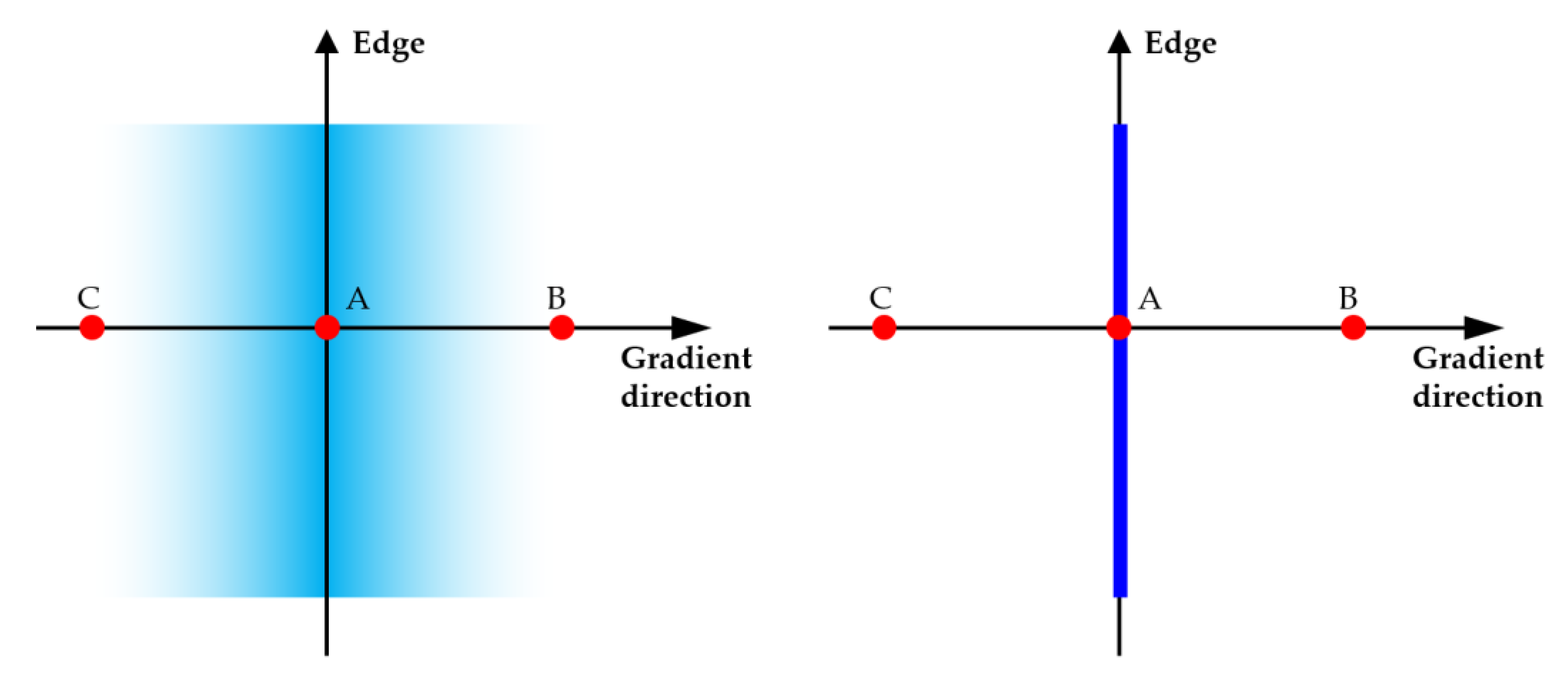
2.1.2. Canny Edge Detection

Canny edge detection, developed by John F. Canny in 1986, is one of the most widely used edge detection algorithms. This algorithm includes a series of noise reduction processes, finding intensity gradients, non-maximum suppression, and hysteresis thresholding [25].

As edge detection is sensitive to image noise, a Gaussian filter can be used to reduce noises. In this study, a $\left(2k+1\right)\times \left(2k+1\right)$ Gaussian kernel was used, as presented in Equation (1) [33]:

$$G_{ij}=\frac{1}{\sqrt{2\pi {\sigma }^2}}{e}^{-\frac{{\left\{i-\left(k+1\right)\right\}}^2+{\left\{j-\left(k+1\right)\right\}}^2}{2{\sigma }^2}};1\le i, j\le 2k+1,$$

(1)

where $G_{ij}$ is the $\left(i, j\right)$ element of the Gaussian kernel, and $\sigma$ is the standard deviation of the Gaussian kernel elements. The larger the Gaussian kernel size, the lower the detector’s sensitivity to noise. A $5\times 5$ size kernel ($\mathsf{\sigma }=1.4$) was applied as presented in matrix (2):

$$G=\frac{1}{159}\left[\begin{array}{ccccc}2& 4& 5& 4& 2\\ 4& 9& 12& 9& 4\\ 5& 12& 15& 12& 5\\ 4& 9& 12& 9& 4\\ 2& 4& 5& 4& 2\end{array}\right].$$

(2)

By operating Equation (3) on each pixel of the image, Gaussian blurs were processed, and any noise was removed. The weight decreases as the distance $\left(u, v\right)$ between the central position $\left(x, y\right)$ of the kernel and the kernel position $\left(x+u, y+v\right)$ increases.

$$M_{xy}={\left(f\otimes G\right)}_{xy}={\sum }_W{f}_{x+u, y+v}·G_{uv},$$

(3)

where $M_{xy}$ is the element of the processed image from the data matrix $f$.

The gradient of the image in which the noise has been removed by a Gaussian filter was calculated by applying 3 × 3 size $x$- and $y$-direction Sobel kernels obtained [34] (matrix (4)):

$$G_x=\left[\begin{array}{ccc}-1& 0& 1\\ -2& 0& 2\\ -1& 0& 1\end{array}\right], G_y=\left[\begin{array}{ccc}1& 2& 1\\ 0& 0& 0\\ -1& -2& -1\end{array}\right],$$

(4)

where $G_x$ and $G_y$ are the $x$- and $y$-directions of the Sobel kernel, respectively. The filter was applied using Equation (3) similarly to the Gaussian filter.

After that, the edge gradient and direction of each pixel were calculated using Equations (5) and (6):

$$G=\sqrt{G_x^2+G_y^2},$$

(5)

$$\theta ={\tan }^{-1}\left(\frac{G_y}{G_x}\right),$$

(6)

where $G$ is the edge gradient of each pixel, and $\theta$ is the direction of the edge gradient. The entire image was searched in the gradient’s direction to find pixels with the maximum value of the gradient values, representing the edge. Pixels with smaller values than the maximum were then removed by nullifying those pixels with zero value (Figure 1).

Hysteresis thresholding was used to determine whether the result of non-maximum suppression represents a definite edge. Two threshold values were set as the ‘high’ and ‘low’ thresholds. Edges composed of pixels with values greater than the ‘high’ threshold were considered as valid, while edges with values smaller than the ‘low’ threshold were thought to be invalid and, thus, removed. When a pixel value was between the ‘high’ and ‘low’ thresholds, the edges were valid only if connected to a pixel with a value above the ‘high’ threshold.

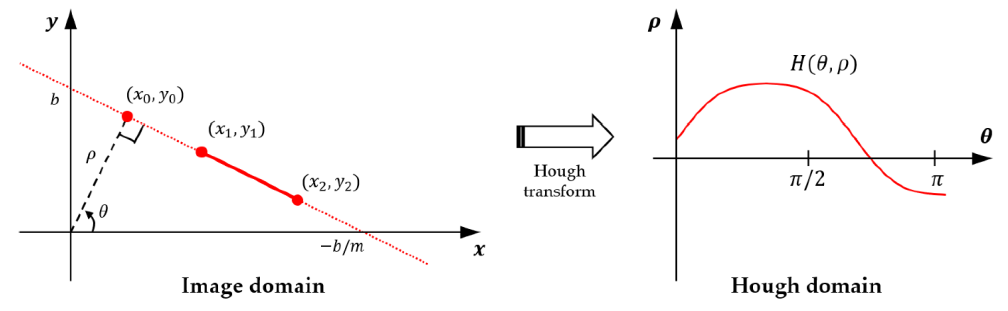
2.1.3. Hough Transform

The Hough transform is a method to extract straight lines by finding correlations between specific points on a Cartesian coordinate plane in digital image processing [35]. In the Cartesian coordinate system, a straight line with slope $m$ and $y$-intercept $b$ can be uniquely expressed as Equation (7):

$$y=mx+b,$$

(7)

where $m$ represents the line slope in the Cartesian coordinates and $b$ is the $y$-intercept of the line. This straight line can be expressed as the coordinates $\left(b, m\right)$ in the parameter space. However, a straight line in the form $x=\mathrm{constant}$ causes divergences and the slope parameter $m$ becomes infinity. Therefore, for computational reasons, Richard and Peter [36] proposed using a Hessian standard form as

$$\rho =x\cos \theta +y\sin \theta ,$$

(8)

where$\rho$ is the distance between the origin and the line and$\theta$ is the radius angle of the line’s normal vector.

When the graph representing Equation (7) for a pair of points $\left(x_1, y_1\right)$ and $\left(x_2, y_2\right)$ is plotted in Hough space, it becomes a sinusoidal curve (Figure 2), which represents all straight lines passing through $\left(x_0, y_0\right)$. When applied to all possible pairs of points, the number of graphs passing through the intersection of sinusoidal curves in Hough space indicates the number of points on a straight line. In other words, the junction of $n$ curves at a single point in Hough space indicates $n$ number of points on a straight line in the Cartesian coordinates.

Therefore, detecting a straight line is possible by obtaining the $\left(\rho ,\theta \right)$ of a straight line passing through any two points $\left(x_i, y_i\right)$ and $\left(x_j, y_j\right);i\ne j$ in the point set $S=\left\{\left(x_i, y_i\right)\right\} ;i\in \mathbb{N}$ of the binary image, and by determining that $\left(\rho ,\theta \right)$ appearing with a high frequency is a real straight line.

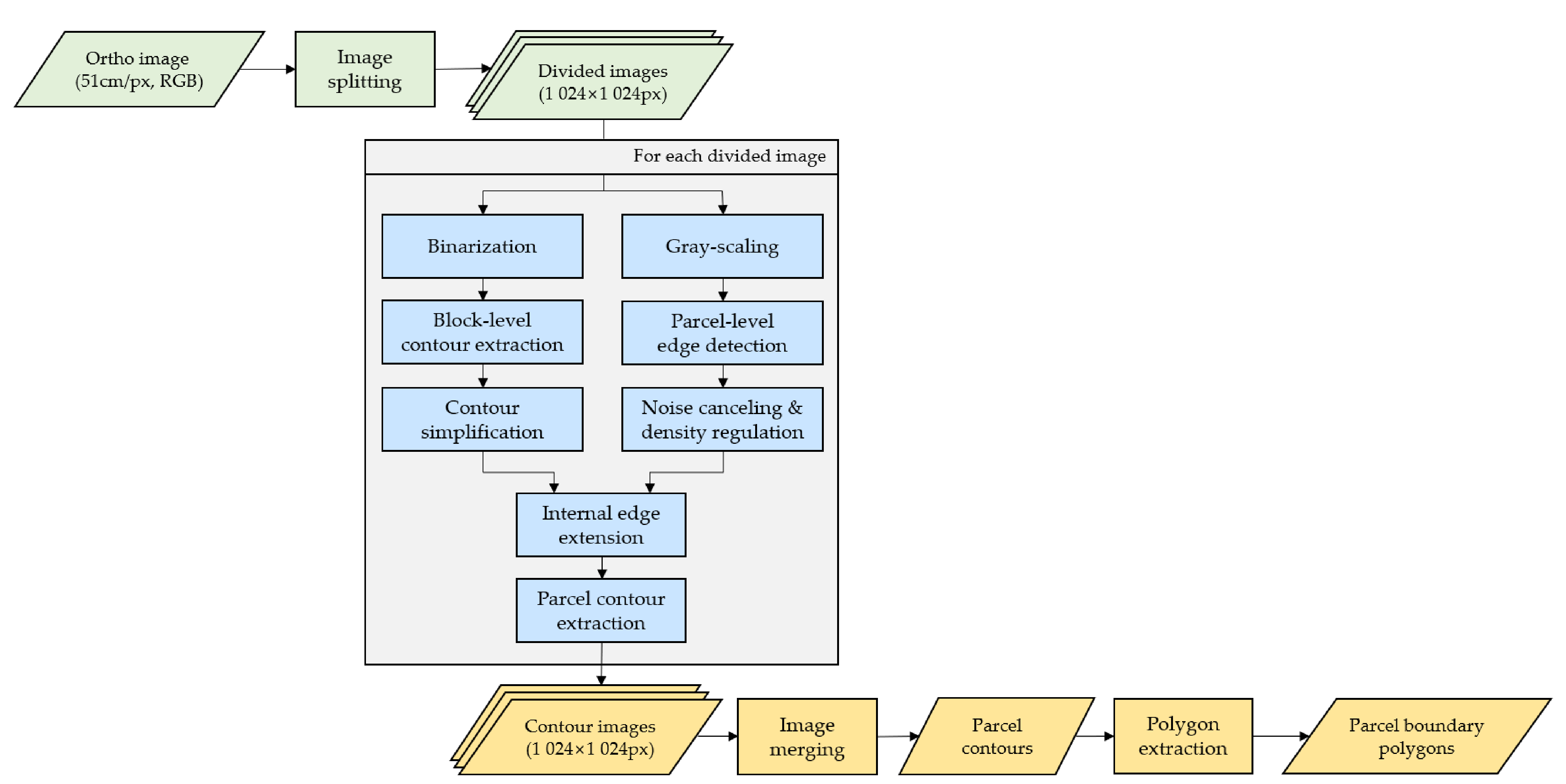
2.2. Development of a Parcel Boundary Extraction Algorithm

The developed parcel boundary extraction algorithm consisted of image splitting, parcel contour detection, and image merging (Figure 3).

Orthographic imageries of the study area obtained from the National Geographic Information Institute (NGII) in Korea were used as input data. These are public data produced through both geometric and orthometric correction of aerial photographs under ‘Regulations on Aerial Photography Work (Notification No. 2016-2609 of NGII)’ and ‘Regulations on Imagery Map Production (Notification No. 2016-429 of NGII)’.

The resolution of the orthographic imagery was 51 cm/pixel. Block-level contours were detected using the Suzuki85 algorithm. Most consolidated paddies and uplands had a regular arrangement in the rectangular form. Thus, based on the assumption that the boundaries dividing the parcels are composed of straight lines, the Hough transform was applied to detect parcel-level edges as straight-line forms. These were extended to block-level contours. The Suzuki85 algorithm was reapplied to derive results grouped in list data structure by the parcel contours.

2.2.1. Image Splitting and Merging

Contour extraction and edge detection algorithms were used to extract high gradient values compared to the overall image characteristics. Thus, these algorithms work better in edge extraction when applied to narrow areas rather than extensive areas. These deductive algorithms also tend to be more sensitive to the distinguishable boundaries from the surrounding land, such as mountains, residential areas, and roads, compared with the boundaries of agricultural land, such as paddies and uplands. Therefore, it is advantageous to apply the algorithm to segmented images of an appropriate size to extract the land parcel boundaries.

As shown in Figure 3, the block-level contours were extracted first, and then the edges of the inner land parcels were suppressed and extended to the block boundaries. Comparisons between the block-level contours and internal edge list array were made repeatedly to check their match. Another advantage of the use of split image segments was the reduction of the comparison operations to increase the algorithm’s computational efficiency.

In this study, original aerial imagery was split into several segments of the same size before applying the algorithms. This was because division to the same sized pieces allowed consistent results over the entire image points when using a fixed threshold value. The original image was divided into approximately 1024 pixels size in width and height, as specified in the algorithm. After the edge detections were performed on each segmented image, the entire segmented images were re-merged.

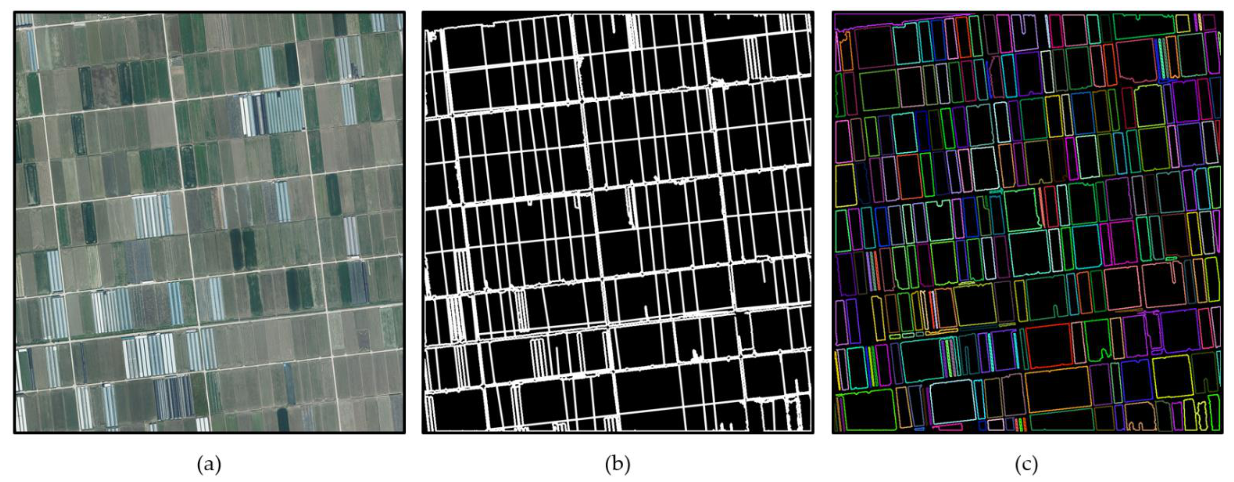
2.2.2. Block-Level Contour Extraction

To extract the contours representing block-level boundaries, an image was converted into 8-bit grayscale according to the YCbCr color space model by applying Equation (9) [37]. The Y component of this color space, which is the same with the YIQ and YUV models, is used widely in grayscale representation. Then the grayscale was converted to 1-bit monochrome (Figure 4b) using a threshold value (Equation (10)):

$$Y_{xy}=0.299R_{xy}+0.587G_{xy}+0.114B_{xy},$$

(9)

$$B{I}_{xy}=\left\{\begin{array}{c}0\\ 255\end{array}\right.\begin{array}{c};{\mu }_{xy}<T\\ ;{\mu }_{xy}\ge T\end{array},$$

(10)

where $Y_{xy}$ is the luma value (grayscale level) at point $\left(x, y\right)$; $T$is the threshold value for image binarization; $R_{xy}$, $G_{xy}$, and $B_{xy}$ are the red, green, and blue components at point $\left(x, y\right)$ in the red, green, and blue (RGB) image, respectively; and $B{I}_{xy}$ is the value at point $\left(x, y\right)$ in the binary image.

When a fixed value is applied to the binarization process threshold, the threshold setting can be out of range for a particular circumstance that causes process errors. To solve this problem, threshold values for the binarization of segmented images were determined in such a way that the intra-class variance (Equation (11)) was minimized or inter-class variance (Equation (12)) was maximized between classes when the image pixels were classified into two categories, as described by Otsu’s method [38]. Although minimizing intra-class variance is mathematically similar to maximizing inter-class variance, it is computationally efficient to apply Equation (12).

$$\mathrm{Intra}-\mathrm{class} \mathrm{variance}=\alpha {\sigma }_1^2+\beta {\sigma }_2^2,$$

(11)

$$\mathrm{Inter}-\mathrm{class} \mathrm{variance}=\alpha \beta {\left({\mu }_1-{\mu }_2\right)}^2,$$

(12)

where $\alpha$ represents the number of pixels with a value smaller than the threshold, $\beta$ is the number of pixels with a value greater than the threshold, and ${\mu }_1$and ${\sigma }_1$are the average and variance values for pixels smaller than the threshold, while ${\mu }_2$and ${\sigma }_2$are for pixels greater than the threshold, respectively.

The image was then binarized systematically based on the threshold, determined with Equation (12), which maximizes the inter-class variance. After that, block-level contours were extracted using the Suzuki85 algorithm (Figure 4c).

As shown in Figure 4c, all contour lines were extracted without a hierarchy relationship. A minimum number of pixels to draw a contour line was applied to extract the block boundaries while minimizing the computational memory usage.

The contours extracted from the image contained detailed coordinate information regarding the shape of objects. These contours were simplified into polygons by removing redundant coordinates using the Ramer–Douglas–Peuker algorithm [39,40]. All extracted contours were pruned into more straightforward object boundaries by using the maximum distance limit around 0.0001. The final contour line was determined as the inner area of a contour approximated to the image block’s size (Figure 4d).

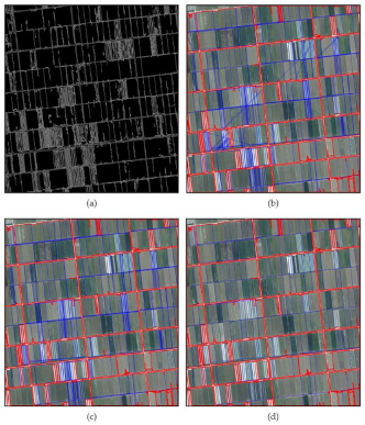
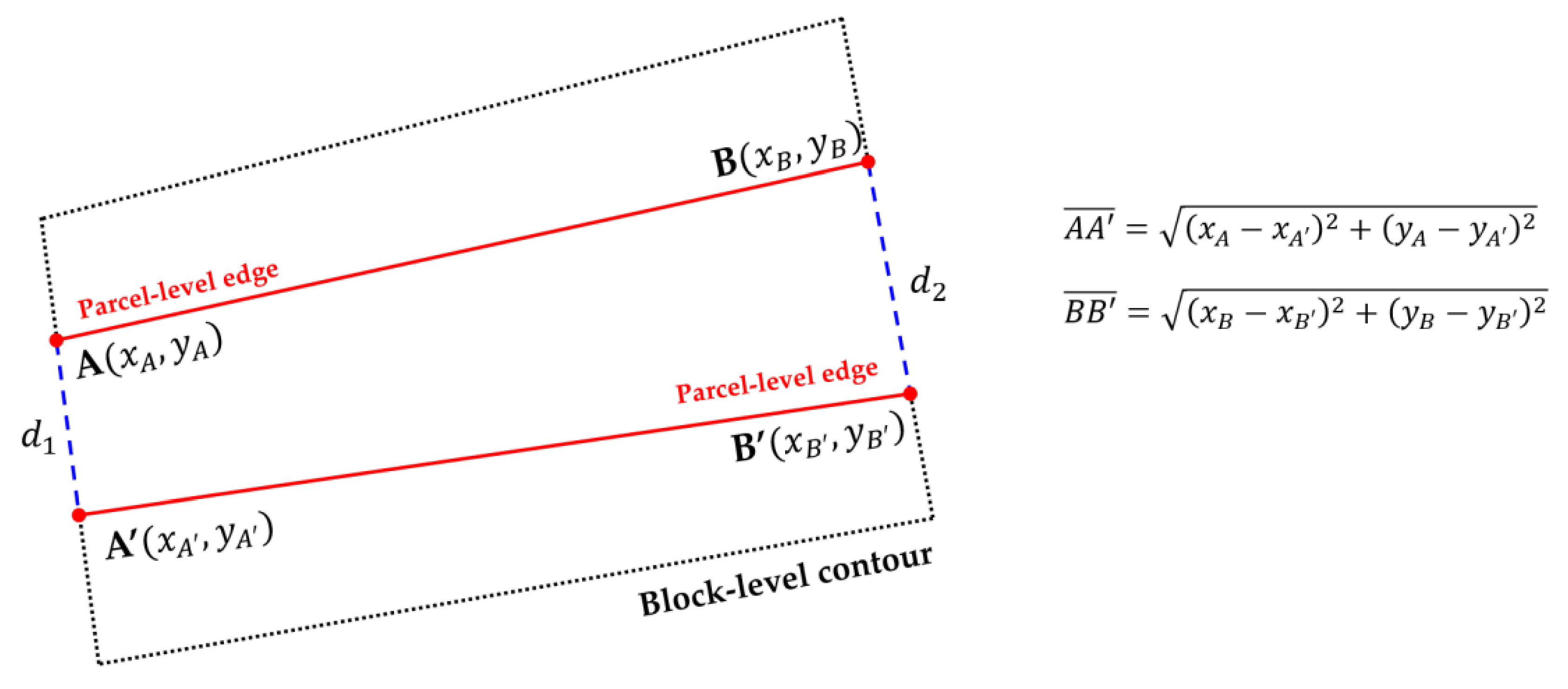
2.2.3. Parcel-Level Edge Extraction from Block-Level Contours

The Canny edge detection algorithm was applied to the grayscale images obtained from Equation (9) (Figure 5a). For paddies and uplands, sensitive edge extraction was required, as both showed a similar intensity in grayscale images. Therefore, a minimum Sobel kernel of 3 × 3 was applied to the gradient calculation (Equation (4)). The values of 80 and 240 were respectively used as low and high hysteresis thresholds through repeated trial and error applications.

The Hough transform was used to extract the parcel edges within the block. Although the Hough transform can be applied to the entirety of pixels within a block, a probabilistic Hough transform that performs a Hough transform on pixels randomly extracted from all target pixels was adopted in this study for computational efficiency. This was because the entire pixel application becomes rapidly inefficient with the increase in image size.

An edge detection resolution of 1-pixel length and 1° angle was set in converting the line segment from the Cartesian coordinate to the Hough domain. Edges with a size less than 25 pixels or within 3 pixels of a mutual distance were ignored, while edges that passed through more than 60 valid pixels were determined as valid.

2.2.4. Parcel Contour Extraction

A specific parcel boundary within a block was extracted by extending a line segment from the Hough transform process to the block contours. The hierarchical relationship between the edges and contours was identified using a ray casting algorithm [41] in combination with a type of inside-polygon test [42] for all pairs of block-level contours and edges within the segment. An arbitrary ray was constructed to cast at a point and determined as the point lying within the contour when the ray meets the contour polygon an odd number of times. The link between the determined points became the parcel and was extended to the contour when both endpoints of the link were within the same block contour. In other words, the edge of either end that was not included in the same block contour was removed (Figure 5b).

To remove noises that did not match the parcel arrangement direction of the inner edges, the angular range $\left[0,\pi \right]$ was divided by $\frac{\mathsf{\pi }}{18}$ rad intervals and the number of edges of each range was determined by calculating all edges’ angles. Based on the regularity of parcel arrangement, only the edges along the direction of the majority of the angular range remained and the other edges with deviated angles were removed (Figure 5c).

The line density was then adjusted by overlapping the inner edges with similar inclinations. The distances of $\overline{{AA}^{\prime }}$ and $\overline{{BB}^{\prime }}$ between both the ends of the two edges $\overline{AB}$ and $\overline{A^{\prime }{B}^{\prime }}$ were calculated (Figure 6), and one edge was removed if both distance values ($\overline{{AA}^{\prime }}, \overline{{BB}^{\prime }}$) were smaller than 5 pixels (Figure 5d). The number of 5 pixels was determined based on trial and error in order to eliminate the redundant finer boundaries as the given resolution of the images used in this study.

The Suzuki85 algorithm was then applied once more to finalize the valid block-level contours and parcel-level edges (Figure 7b). Thereby, all the extracted block-level and parcel-level edges eventually became the parcel-level boundaries, and their coordinate information was stored (Figure 7c).

3. Assessment of Developed Boundary Extraction Algorithm

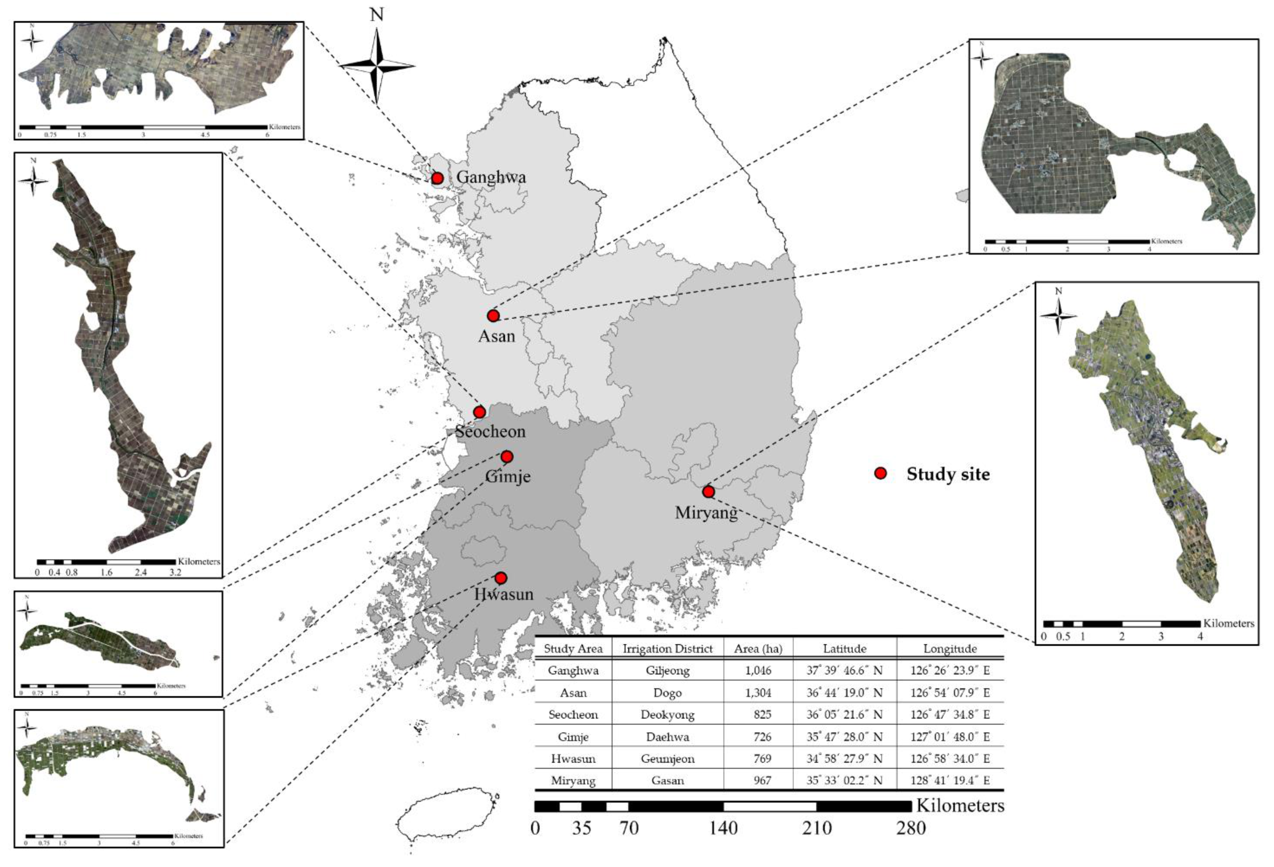
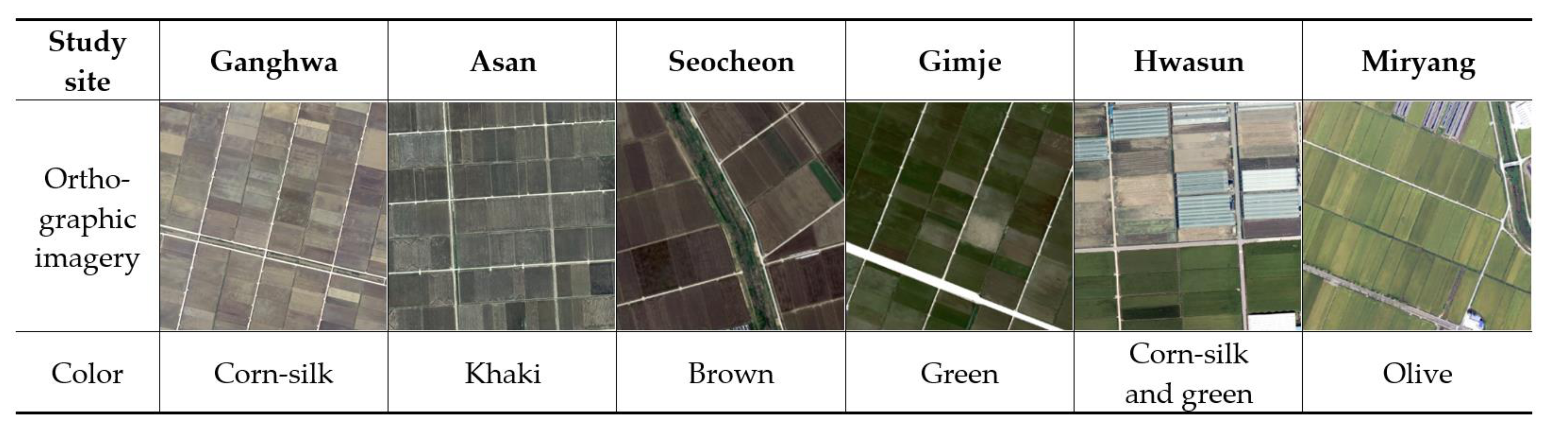
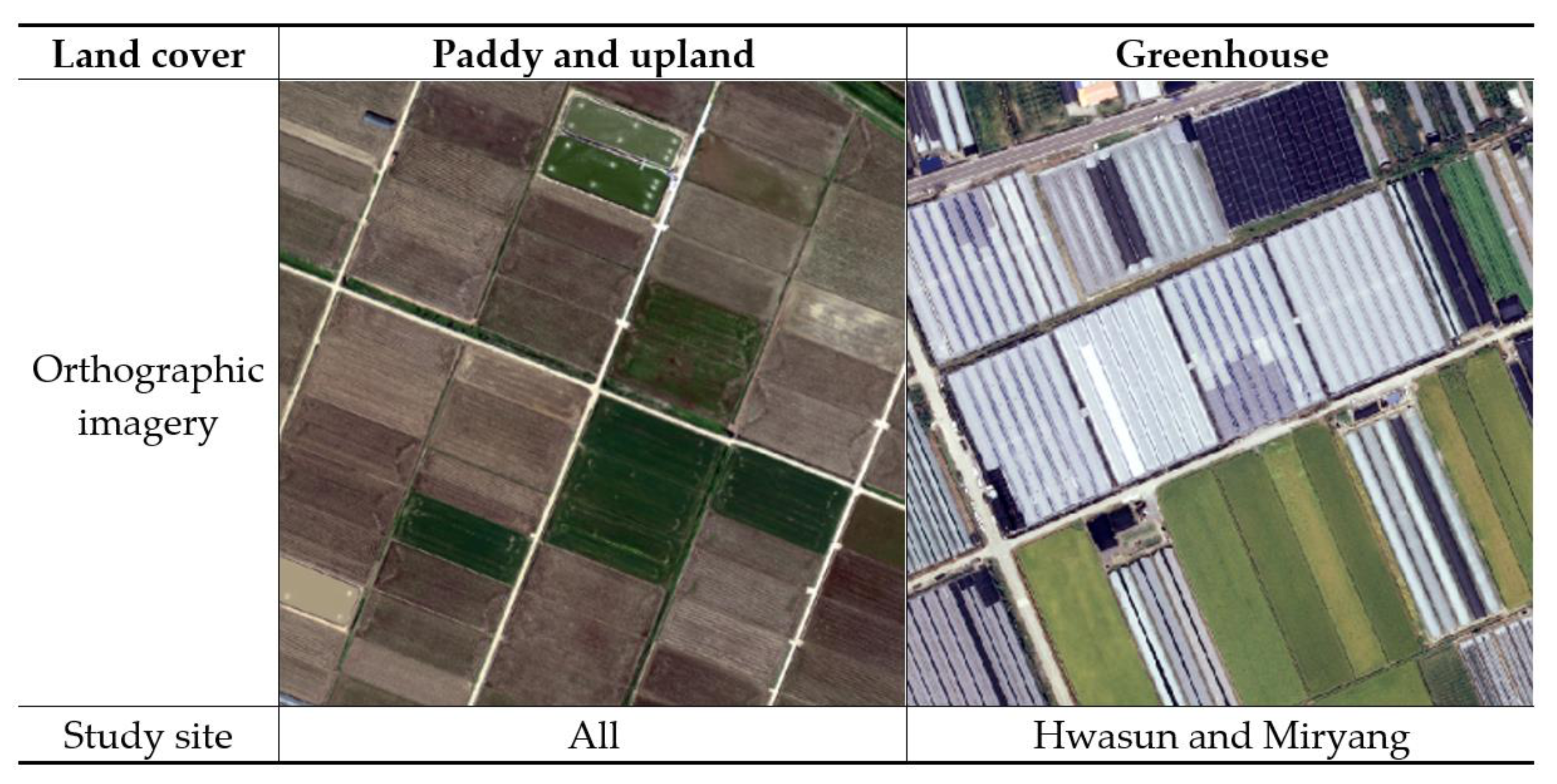
3.1. Study Site

The hues of aerial imagery may vary depending on the surface cover conditions or aerial photographing times. Images of various surface cover conditions are required to evaluate the developed algorithm’s performance in extracting parcel boundaries from aerial images. In this study, six evaluation areas were selected based on the distribution of land parcels, such as paddies, uplands, and greenhouses as well as surface color hues (Figure 8), as edge extraction is highly influenced by the image characteristics of the objects.

The study sites with various surface hues (corn-silk, khaki, brown, green, corn-silk and green, and olive) were selected (Figure 9) to verify the applicability of the developed algorithm for a range of different aerial images. In particular, Hwasun, with two different surface hues of corn-silk and green was included as a study site, since a non-maximum suppression process (Figure 1) through gradient operation tends to be affected heavily by the entire image colors.

The study sites with different land cover types were also selected to evaluate the boundary extraction. All the study sites included paddy and upland as the primary land cover, while the two sites of Hwasun and Miryang were chosen to assess the effect of greenhouse areas on parcel extraction (Figure 10).

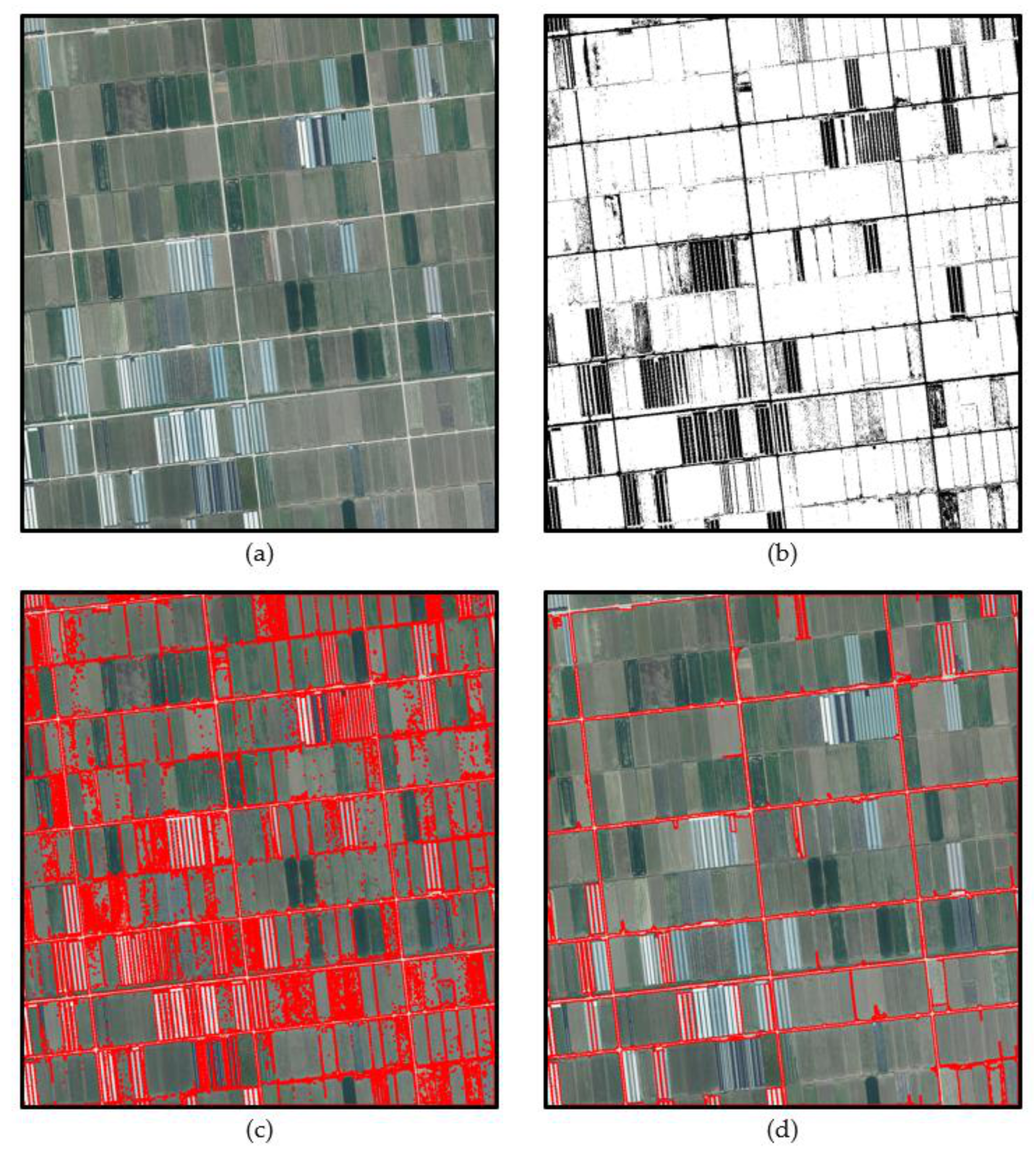
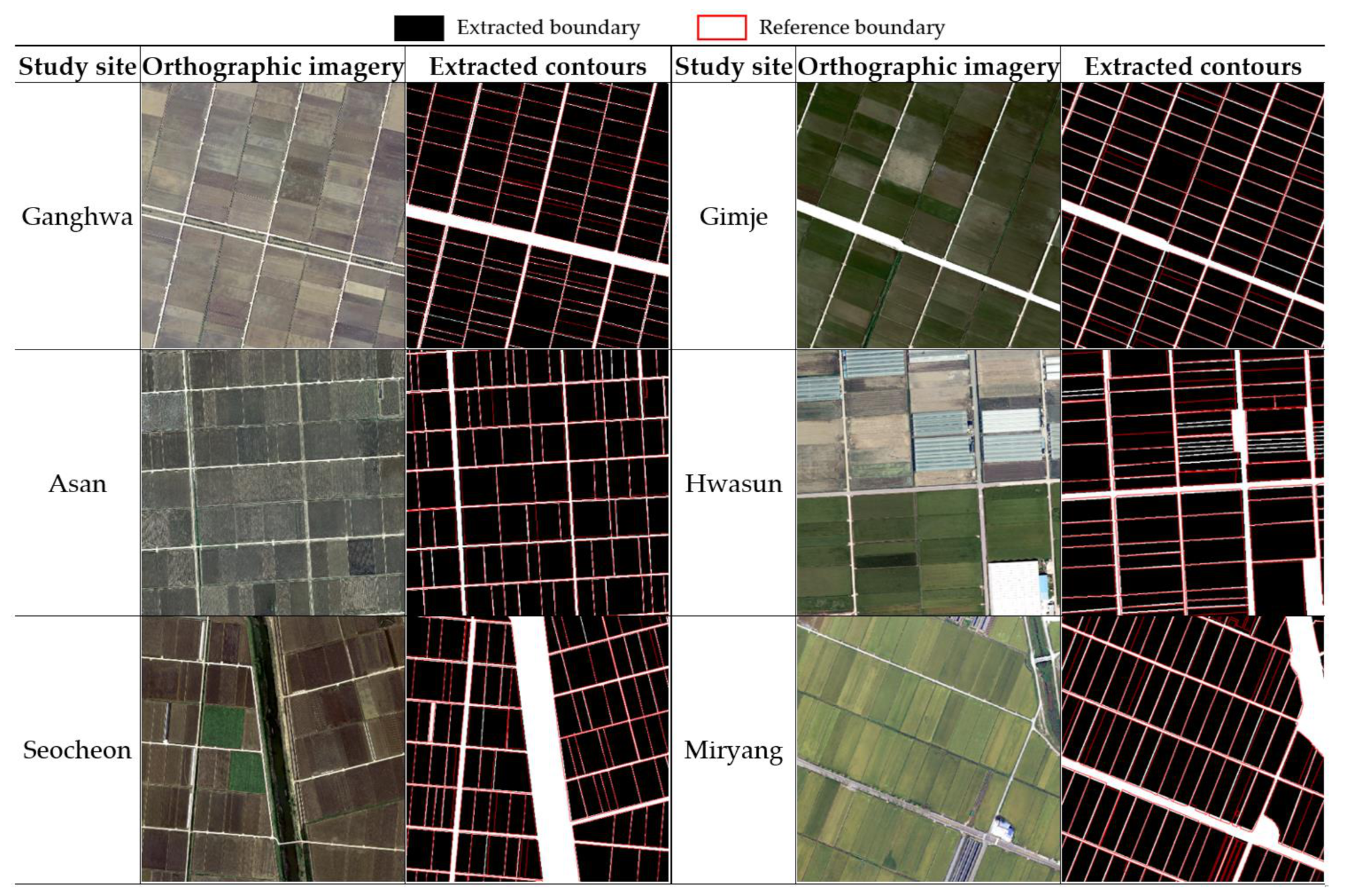
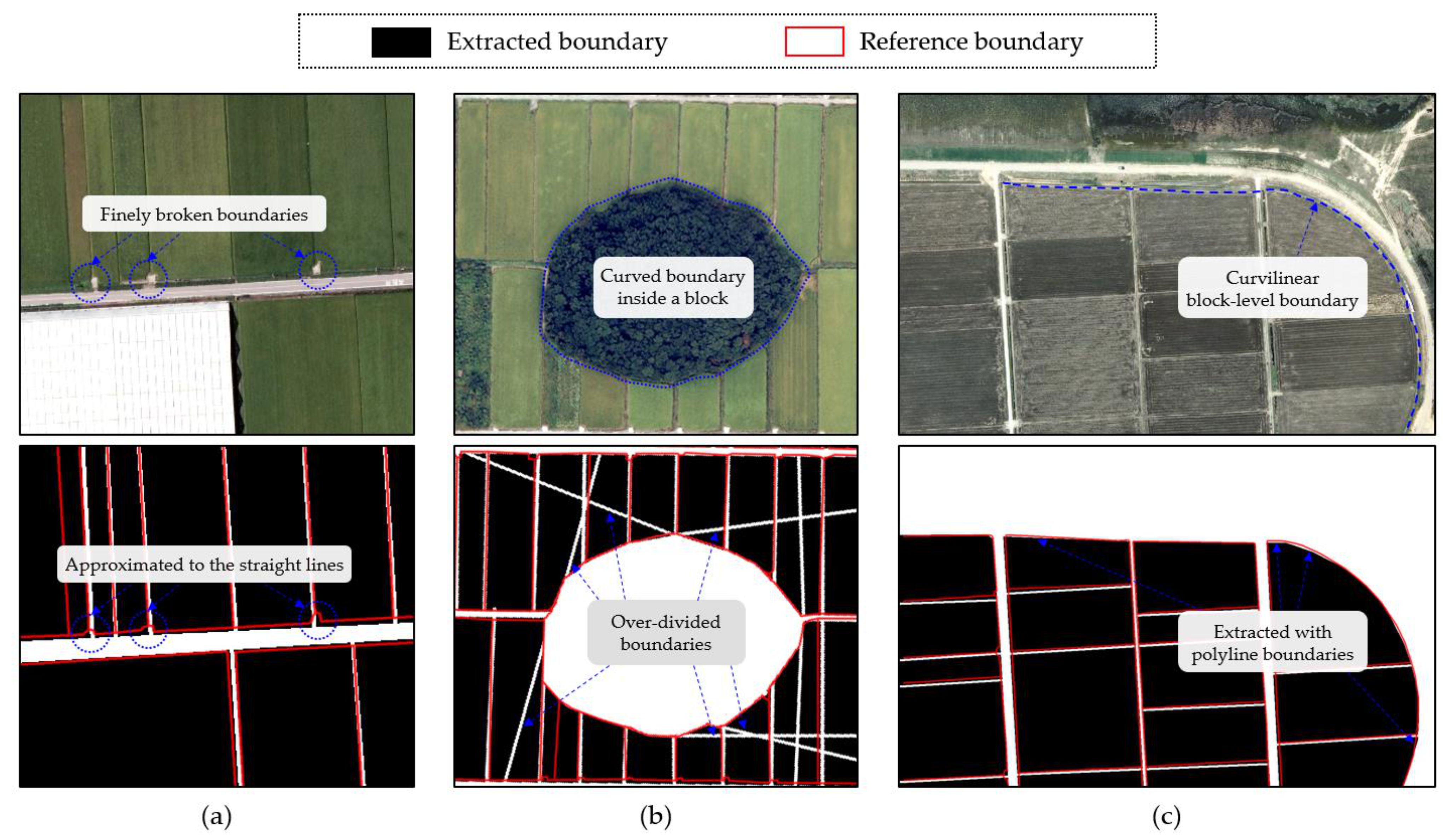
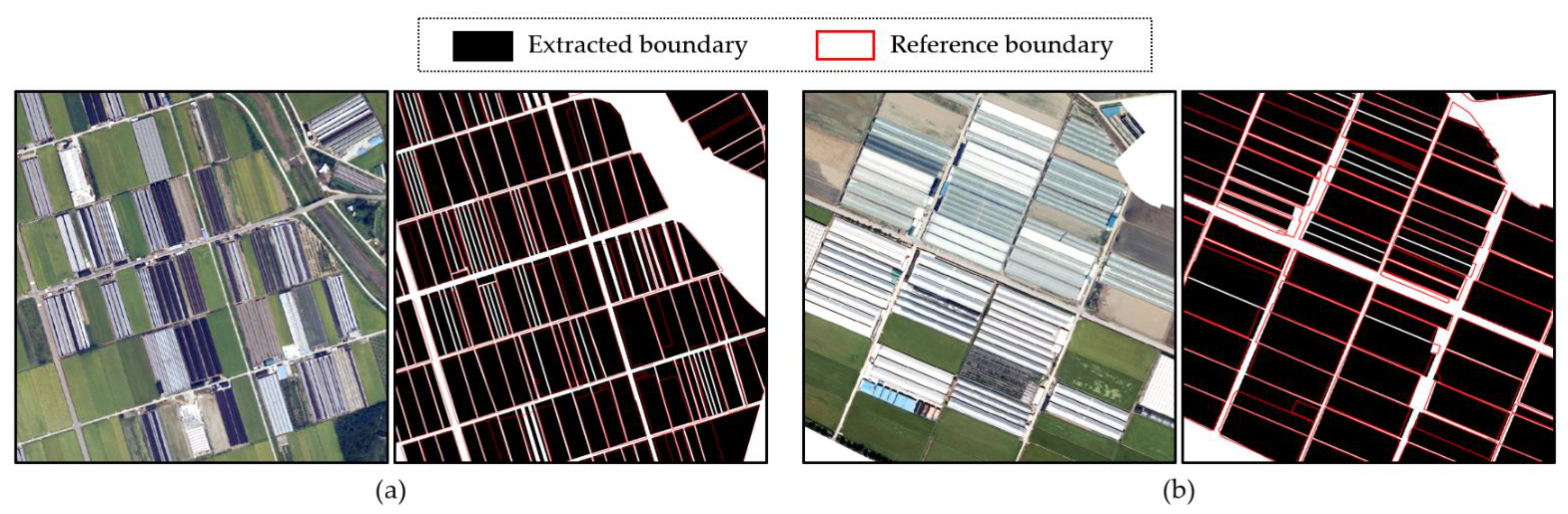
3.2. Parcel Boundary Extraction

As shown in Figure 11, the boundaries between paddy and upland in the original imagery were matched well with the boundaries extracted by the developed algorithm for all the study sites. Although there were rare cases that omitted the boundaries between the parcels with very similar colors, the developed algorithm demonstrated good performance in boundary extraction regardless of the surface color hues, indicating the applicability for different soil colors and aerial photography time.

There are some parcel boundaries that are polyline, arc, and curved line due to various environmental and artificial factors. Thus, some anomalies between a straight line through the Hough transform and the actual parcel boundary shape appeared. The first anomaly was finely broken lines that resulted from farm entry road features (Figure 12a). This can be approximated to a straight line of rectangular boundaries by the density regulation of the parcel contour extraction process. The second anomaly was over-divided boundaries (white lines in Figure 12b). This case was rather rare and occurred when isolated curved features, such as forests or unconsolidated small segments existed within the block-level boundary. Most of these features can be removed by the noise removing process, as described in Section 2.2.4. The third anomaly was curvilinear block-level contours (Figure 12c). This was not affected by the Hough transform and could be well extracted by the Suzuki85 algorithm.

The developed algorithm also performed well in extracting parcel boundaries for the sites with greenhouses by clearly differentiating greenhouses from paddies and uplands (Figure 13). However, the parcels with greenhouses tended to be dissected further with individual greenhouse structures as independent parcels. This is because distinctive greenhouse structures are aligned in parallel to the long side of a land parcel, and thereby the algorithm tends to render individual greenhouses recognizable as independent land parcels. Considering the unique and regular appearance of greenhouses, the identification of an individual greenhouse as a parcel may be agreeable or multiple structures may be merged into a single parcel with an additional algorithm in the future.

3.3. Boundary Extraction Accuracy Assessment

An official farm map was used as the reference land parcel boundary data for the algorithm performance assessment. The farm map is the electronic version of the national farmland registration provided by the Ministry of Agriculture, Food and Rural Affairs of Korea. This map was generated and regularly updated by onscreen manual digitizing of farmland information using the aerial photographs and the national cadastral map along with extensive field inspection for verification. Four different major farm categories of paddies, uplands, orchards, and greenhouses were established in the farm map as the shape data.

The algorithm’s parcel boundary extraction performance was evaluated in two aspects: the boundaries themselves and the sections formed by the boundaries.

3.3.1. Matching the Extracted Boundaries with the Reference Boundaries

The boundary of a parcel extracted by the developed algorithm must match with the respective boundary in the farm map for the evaluation of the model accuracy. For this, the maximum overlap area method was applied to compute the coincidence degree $O_{ij}$ between two boundaries consisting of all the extracted and the reference [43]:

$$O_{ij}=\frac{1}{2}\left(\frac{A_{e,i}\cap A_{r,j}}{A_{e,i}}+\frac{A_{e,i}\cap A_{r,j}}{A_{r,j}}\right),$$

(13)

where $A_{e,i}$ denotes the area of the $i\mathrm{th} \mathrm{extracted} \mathrm{boundary}$, $A_{r,j}$ is the area of the $j$th reference boundary. The one with the maximum coincidence degree among the extracted boundaries was matched to the respective reference boundary.

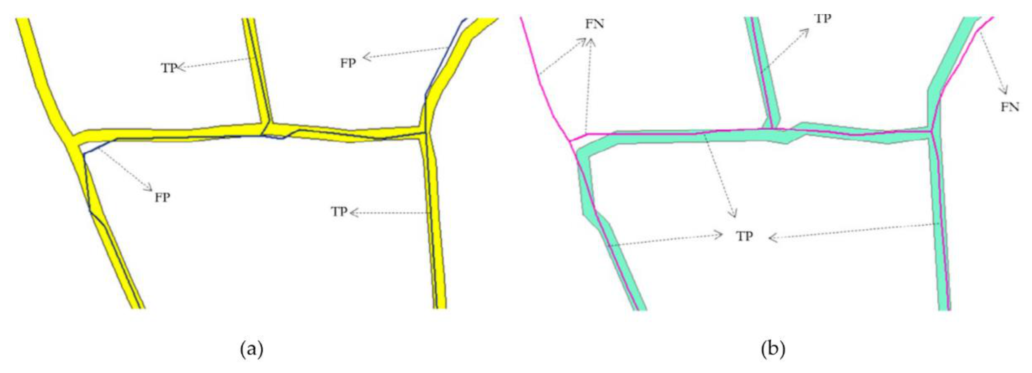
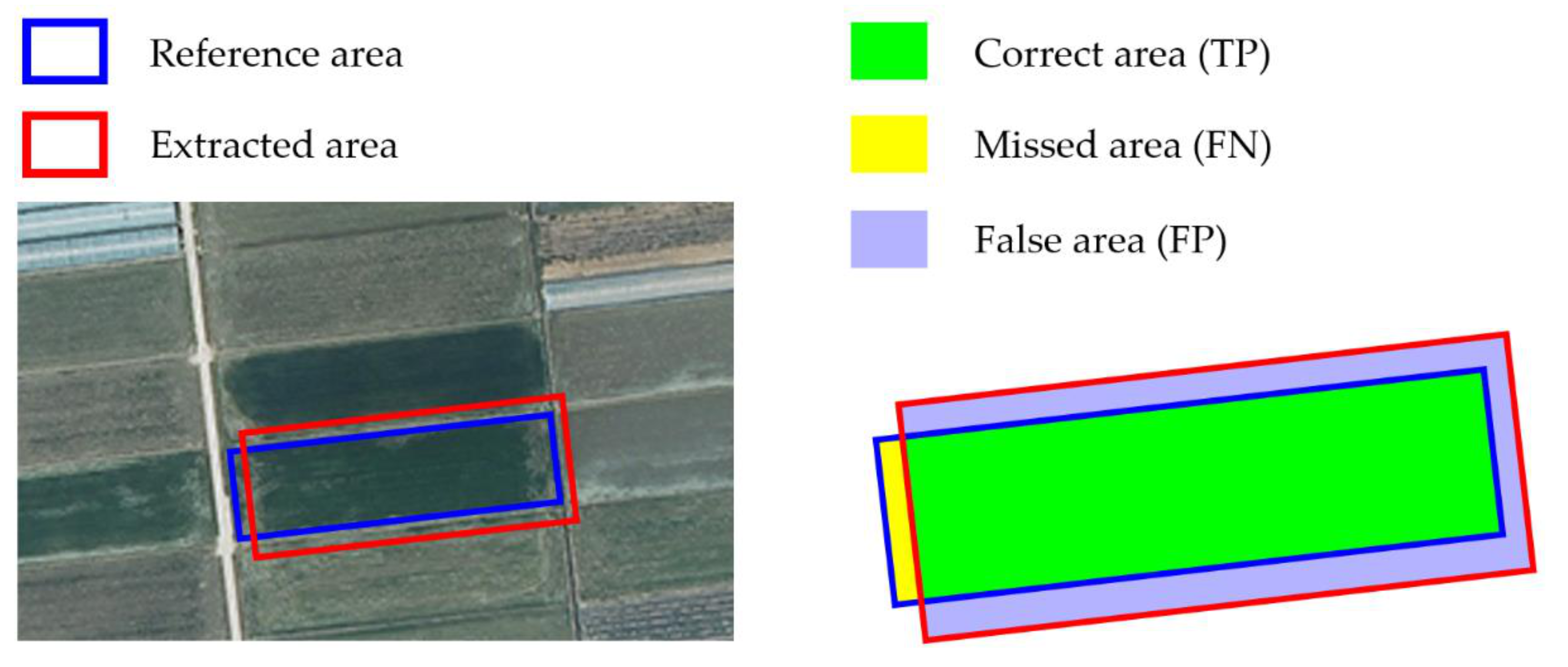
3.3.2. Boundary Level Accuracy Assessments

The extracted boundaries were assessed quantitatively by applying a buffer overlay method [44,45,46]. When the extracted boundaries are overlaid to the buffer around the reference boundaries, the overlapping ones on the buffer are true positive (TP), otherwise FP. Similarly, by overlaying the reference boundaries on the buffer around the extracted boundaries, true negative (TN) and false negative (FN) were determined. TP, FP, FN, and TN are demonstrated in

Table 1. Definitions of true positive, false positive, false negative, and true negative results regarding the extracted results and the reference.

Reference	Extracted Results
	Positive	Negative
Positive	True positive (TP, correct)	False negative (FN, missed)
Negative	False positive (FP, false)	True negative (TN)

and Figure 14 [47].

The International Association on Assessing Officers (IAAO) proposed a buffer width limit of 2.4 m for sufficient accuracy in the boundaries of rural areas [48]. A buffer width of 2.0 m was used in this study. TP, FP, and FN were calculated by converting the extracted (or reference) polygon boundaries into line features and overlaying this on the buffer of the paired reference (or extracted) boundaries. The calculated lengths of TP, FP and FN were then used to evaluate the completeness, correctness, and quality of the extracted boundaries using Equations (14)–(16):

$$\mathrm{Correctness}=\frac{\mathrm{TP}}{\mathrm{TP}+\mathrm{FP}},$$

(14)

$$\mathrm{Completeness}=\frac{\mathrm{TP}}{\mathrm{TP}+\mathrm{FN}},$$

(15)

$$\mathrm{Quality}=\frac{\mathrm{TP}}{\mathrm{TP}+\mathrm{FP}+\mathrm{FN}}.$$

(16)

Each indicator has a value between 0 and 1, and the closer to 1, the better the algorithm’s performance. The correctness, completeness, and quality of the extracted boundaries were calculated for the entire parcels of the respective study sites and are presented in

Table 2. The correctness, completeness, and quality of the extracted boundaries.

Study Site	Correctness (%)	Completeness (%)	Quality (%)
Ganghwa	82.8	82.7	70.6
Asan	80.9	79.9	67.3
Seocheon	83.9	83.4	71.9
Gimje	81.4	81.0	68.3
Hwasun	77.2	73.9	60.6
Miryang	77.6	77.4	63.3
Mean	80.7	79.7	67.0

.

In general, correctness showed a greater value compared with completeness, which is expected because the reference boundaries better reflect the non-smooth curves of reality. In particular, the correctness, completeness, and quality for the Hwasun and Miryang sites, which included greater areas of greenhouses, appeared to be relatively low. Greenhouses have distinctive image characteristics compared to paddies and uplands that lead to clear identification and more subdivision of the boundaries between greenhouses compared with the reference boundaries (Figure 13). This was the primary reason for the high rates of FP and FN, resulting in smaller values of quality of the extracted boundaries. The mean correctness, completeness, and quality over the six study sites were 80.7%, 79.7%, and 67.0%, respectively. Considering the previous study results with the respective values of 73.3%, 73.0%, and 59.7% by Khadanga et al. [17], the developed algorithm performed reasonably well in boundary extraction.

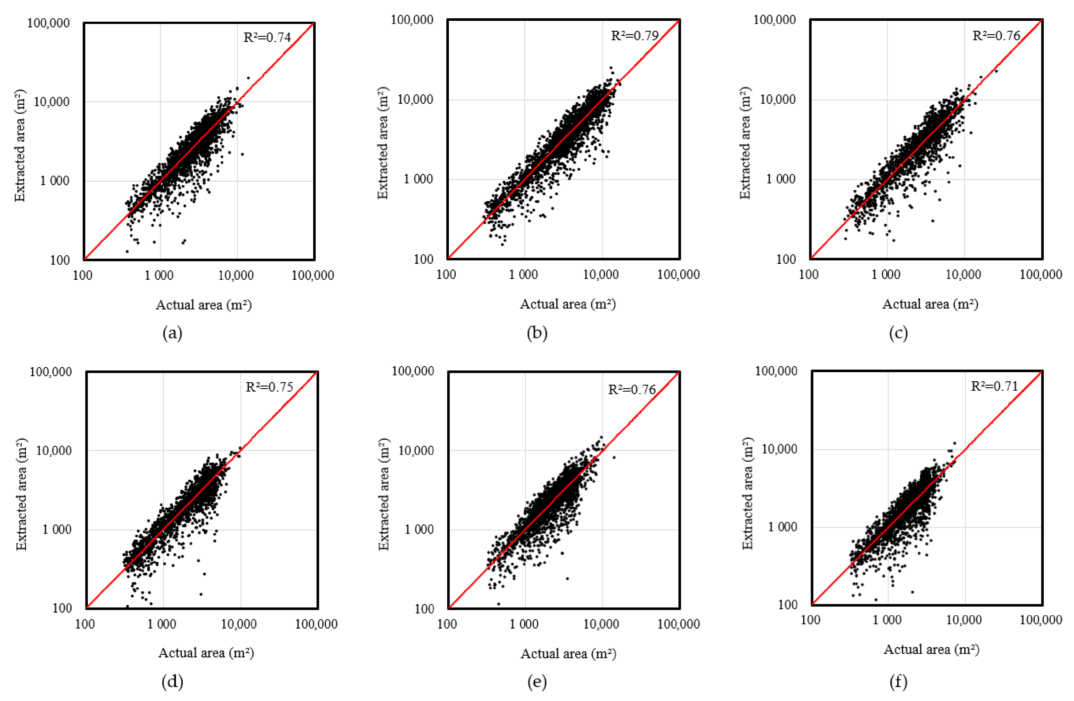
3.3.3. Section Level Accuracy Assessments

To analyze the developed algorithm’s accuracy on the section level, two measures in terms of the area and the number of extracted boundaries were applied. These measures are methods that can be used to analyze the accuracy of single feature extraction, such as boundary extraction based on object-based image analysis (OBIA) [43].

The area-based accuracy assessment method measured the correctness, completeness, and quality of the extracted boundaries. These were calculated using Equations (14)–(16) for the entire parcels based on the results exemplified in Table 1 and Figure 15.

The correctness, completeness, and quality of the extracted sections were calculated for the entire parcels of the respective study sites and are presented in

Table 3. Area-based accuracy measures of the extracted sections.

Study Site	Total Area of Parcels (m2)			Correctness (%)	Completeness (%)	Quality (%)
	Reference	Extracted	Correct
Ganghwa	6,809,013	6,839,701	6,213,570	90.8	91.3	83.6
Asan	10,480,100	10,600,606	9,493,488	89.6	90.6	81.9
Seocheon	5,172,362	5,191,725	4,672,918	90.0	90.3	82.1
Gimje	4,335,019	4,344,432	3,991,849	91.9	92.1	85.2
Hwasun	5,607,757	5,613,631	4,895,097	87.2	87.3	77.4
Miryang	5,145,164	5,142,539	4,558,913	88.7	88.6	79.6
Mean				89.7	90.0	81.6

.

The mean correctness, completeness, and quality of the area-based assessments were 89.7%, 90.0%, and 81.6%, respectively, indicating good performance of the algorithm. Some of the overly dissected parcels were removed during the density regulation process, while thresholding resulted in a reduction of completeness and quality.

The number-based accuracy assessment method measured the correct, false, and missing rates relying on the number of boundaries. Each measure had a value between 0 and 1, and these were calculated as:

$$\mathrm{Correct} \mathrm{rate}=\frac{N_c}{N_c+N_f},$$

(17)

$$\mathrm{False} \mathrm{rate}=\frac{N_f}{N_c+N_f},$$

(18)

$$\mathrm{Missing} \mathrm{rate}=\frac{N_m}{N_c+N_m},$$

(19)

where $N_c$, $N_f$, and $N_m$ denote the number of correct, false, and missed extracted boundaries. The closer the correct rate was to 1, and the closer to 0 for false and missing rates, the better the algorithm’s performance. The coincidence degree was applied as a criterion for determining whether the extracted boundary was correct, false, or missed. These were determined based on a coincidence degree threshold value of 0.8, and the extracted boundary that was not matched to the reference boundary was determined as false. The correct, false, and missing rates for each study site were calculated based on the number of correct, false, and missed boundaries (

Table 4. Number-based accuracy measures of the extracted sections.

Study Site	Number of Parcels				Correct Rate (%)	False Rate (%)	Missing Rate (%)
	Reference	Correct	False	Missed
Ganghwa	2384	2113	252	276	89.3	10.7	11.6
Asan	2582	2236	259	275	89.6	10.4	11.0
Seocheon	1653	1508	179	144	89.4	10.6	8.7
Gimje	1798	1617	186	167	89.7	10.3	9.4
Hwasun	2263	1903	315	224	85.8	14.2	10.5
Miryang	2619	2159	347	210	86.2	13.8	8.9
Mean					88.3	11.7	10.0

).

The mean values of number-based indicators were 88.3%, 11.7%, and 10.0% for correct, false, and missing rates, respectively. The overall percentage of falsely extracted boundaries was relatively greater for the Hwasun and Miryang sites, which contained greater areas of greenhouses. Scatter plots of the reference areas against the extracted areas were well aligned along the 1:1 line, as shown in Figure 16. However, the sizes of the reference parcel boundary appeared to be consistently greater compared with those of the extracted boundaries for all the study sites. This means that the algorithm tended to subdivide land parcels as compared to the reference area primarily due to the greenhouse structure as aforementioned in Section 3.3.2.

The resulting values of the area- and number-based accuracy measures were comparable with the results of previous studies [17,49,50]. Thus, the developed model can be used to facilitate rapid updates of farm maps through the automation of farmland boundary extraction. However, the current algorithm is only applicable for the regularly arranged land parcels and further development is required for more general applications to non-regular shapes of land, possibly with the help of the artificial intelligence.

4. Conclusions

In an effort to automate parcel boundary extraction from aerial images in agricultural areas, we developed a parcel-level boundary extraction algorithm in this study, and its performance was evaluated over six study sites. The set of computational and mathematical methods used for the developed algorithm include the Suzuki85 algorithm, Canny edge detection, and Hough transform.

As for the match-ness assessment between the extracted and reference boundary, the developed algorithm demonstrated 80.7%, 79.7%, and 67.0% correctness, completeness, and quality, respectively. The area-based accuracy measures of correctness, completeness, and quality were 89.7%, 90.0%, and 81.6%, respectively. These results appeared to be comparable or better when compared with the results of the previous studies, and thus the developed algorithm can be used in farmland parcel boundary extraction.

Since the developed algorithm is based on the assumption that land parcel boundaries are straight lines, a cautious approach should be taken in applications with non-regular shaped land parcels. The developed algorithm tended to subdivide land parcels further when distinctive features, such as greenhouse structures or isolated, were land parcels within the land blocks.

The developed boundary extraction algorithm is currently only applicable to regularly arranged agricultural lands. A wide range of applications is possible by selectively extracting the boundaries of various objects as well as agricultural parcels. For applications beyond the regular shaped boundaries, further study, potentially with a decision tree or artificial intelligence, is needed.

References

1. Frédéricque, B.; Daniel, S.; Bédard, Y.; Paparoditis, N. Populating a building multi representation data base with photogrammetric tools: Recent progress. ISPRS J. Photogramm. Remote Sens. 2008, 63, 441–460. [Google Scholar] [CrossRef]
2. Xie, Y.; Weng, A.; Weng, Q. Population estimation of urban residential communities using remotely sensed morphologic data. IEEE Geosci. Remote Sens. Lett. 2015, 12, 1111–1115. [Google Scholar]
3. Crommelinck, S.; Bennett, R.; Gerke, M.; Yang, M.Y.; Vosselman, G. Contour Detection for UAV-Based Cadastral Mapping. Remote Sens. 2017, 9, 171. [Google Scholar] [CrossRef] [Green Version]
4. Fetai, B.; Oštir, K.; Kosmatin Fras, M.; Lisec, A. Extraction of Visible Boundaries for Cadastral Mapping Based on UAV Imagery. Remote Sens. 2019, 11, 1510. [Google Scholar] [CrossRef] [Green Version]
5. Paravolidakis, V.; Ragia, L.; Moirogiorgou, K.; Zervakis, M.E. Automatic coastline extraction using edge detection and optimization procedures. Geosciences 2018, 8, 407. [Google Scholar] [CrossRef] [Green Version]
6. Turker, M.; Kok, E.M. Field-based sub-boundary extraction from remote sensing imagery using perceptual grouping. ISPRS J. Photogramm. Remote Sens. 2013, 79, 106–121. [Google Scholar] [CrossRef]
7. Yan, L.; Roy, D.P. Automated crop field extraction from multi-temporal web enabled Landsat data. Remote Sens. Environ. 2014, 144, 42–64. [Google Scholar] [CrossRef] [Green Version]
8. Cho, H.B.; Lee, K.I.; Choi, H.S.; Cho, W.S.; Cho, Y.W. Extracting building boundary from aerial LiDAR points data using extended χ algorithm. J. Korean Soc. Surv. Geod. Photogram. Cartogr. 2013, 31, 111–119. [Google Scholar] [CrossRef] [Green Version]
9. Lee, J.H.; Kim, Y.I. Extraction and modeling of curved building boundaries from airborne lidar data. J. Korean Soc. Geospat. Inf. Syst. 2012, 20, 117–125. [Google Scholar]
10. Segl, K.; Kaufmann, H. Detection of small objects from high-resolution panchromatic satellite imagery based on supervised image segmentation. IEEE Trans. Geosci. Remote Sens. 2001, 39, 2080–2083. [Google Scholar] [CrossRef]
11. Da Costa, J.P.; Michelet, F.; Germain, C.; Lavialle, O.; Grimier, G. Delineation of vine parcels by segmentation of high resolution remote sensed images. Precis Agric. 2007, 8, 95–110. [Google Scholar] [CrossRef]
12. Yang, G.; Zhang, Q.; Zhang, G. EANet: Edge-Aware Network for the extraction of buildings from aerial images. Remote Sens. 2020, 12, 2161. [Google Scholar] [CrossRef]
13. Rabbi, J.; Ray, N.; Schubert, M.; Chowdhury, S.; Chao, D. Small-object detection in remote sensing images with end-to-end edge-enhanced GAN and object detector network. Remote Sens. 2020, 12, 1432. [Google Scholar] [CrossRef]
14. Nguyen, T.H.; Daniel, S.; Guériot, D.; Sintès, C.; Le Caillec, J.-M. Super-resolution-based snake model—An unsupervised method for large-scale building extraction using airborne LiDAR data and optical image. Remote Sens. 2020, 12, 1702. [Google Scholar] [CrossRef]
15. Kass, M.; Witkin, A.; Terzopoulos, D. Snakes: Active contour models. Int. J. Comput. Vis. 1988, 1, 321–331. [Google Scholar] [CrossRef]
16. Xu, C.; Prince, J.L. Snakes, shapes, and gradient vector flow. IEEE Trans. Image Process. 1998, 7, 359–369. [Google Scholar]
17. Khadanga, G.; Jain, K. Cadastral parcel boundary extraction from UAV images. J. Indian Soc. Remote Sens. 2020. [Google Scholar] [CrossRef]
18. North, H.C.; Pairman, D.; Belliss, S.E. Boundary delineation of agricultural fields in multitemporal satellite imagery. IEEE J. Sel. Top. Appl. Earth Obs. Remote Sens. 2019, 12, 237–251. [Google Scholar] [CrossRef]
19. Wagner, M.P.; Oppelt, N. Extracting agricultural fields from remote sensing imagery using graph-based growing contours. Remote Sens. 2020, 12, 1205. [Google Scholar] [CrossRef] [Green Version]
20. Kang, M.S.; Park, S.W.; Yoon, K.S. Land cover classification of image data using artificial neural networks. J. Korean Soc. Rural Plan. 2006, 12, 75–83. [Google Scholar]
21. Park, J.; Jang, S.; Hong, R.; Suh, K.; Song, I. Development of land cover classification model using AI based FusionNet network. Remote Sens. 2020, 12, 3171. [Google Scholar] [CrossRef]
22. García-Pedrero, A.; Gonzalo-Martin, C.; Lillo-Saavedra, M. A machine learning approach for agricultural parcel delineation through agglomerative segmentation. Int. J. Remote Sens. 2016, 38, 1809–1819. [Google Scholar] [CrossRef] [Green Version]
23. Waldner, F.; Diakogiannis, F.I. Deep learning on edge: Extracting field boundaries from satellite images with a convolutional neural network. Remote Sens. Environ. 2020, 245, 111741. [Google Scholar] [CrossRef]
24. Suzuki, S.; Abe, K. Topological structural analysis of digitized binary images by border following. Comput. Vis. Graph. Image Process. 1985, 30, 32–46. [Google Scholar] [CrossRef]
25. Canny, J. A Computational approach to edge detection. IEEE Trans. Pattern Anal. Mach. Intell. 1986, 8, 679–698. [Google Scholar] [CrossRef]
26. Hough, P.V.C. Method and Means for Recognizing Complex Patterns. U.S. Patent 3,069,654, 28 December 1962. [Google Scholar]
27. Pratt, W.K. Digital Image Processing: PIKS Scientific Inside, 3rd ed.; John Wiley and Sons, Inc.: New York, NY, USA, 2001; p. 736. [Google Scholar]
28. Hlavac, V.; Sonka, M.; Boyle, R. Image Processing, Analysis, and Machine Vision; Springer: Boston, MA, USA, 1993; pp. 112–191. [Google Scholar]
29. Rajashekar, P. Evaluation of stopping criterion in contour tracing algorithms. Int. J. Comput. Sci. Inf. Technol. 2012, 3, 3888–3894. [Google Scholar]
30. Pavlidis, T. Algorithms for Graphics and Image Processing, 1st ed.; Springer: Berlin/Heidelberg, Germany; New York, NY, USA, 1982; p. 438. [Google Scholar]
31. Bradski, G. The OpenCV Library. Dr. Dobb’s J. Softw. Tools 2000, 5, 120–125. [Google Scholar]
32. Lee, D.Y.; Shin, D.K.; Shin, D.I. A finger counting method for gesture recognition. J. Internet Comput. Serv. 2016, 17, 29–37. [Google Scholar] [CrossRef] [Green Version]
33. Hagen, N.; Decennia, E.L. Gaussian profile estimation in two dimensions. Appl. Opt. 2008, 47, 6842–6851. [Google Scholar] [CrossRef]
34. Dim, J.R.; Takamura, T. Alternative approach for satellite cloud classification: Edge gradient application. Adv. Meteorol. 2013, 2013, 1–8. [Google Scholar] [CrossRef] [Green Version]
35. Lee, H.W. Modified canny edge detection algorithm for detecting subway platform screen door invasion. J. Korea Inst. Electron. Commun. Sci. 2019, 14, 663–670. [Google Scholar]
36. Richard, O.D.; Peter, E.H. Use of the Hough transformation to detect lines and curves in pictures. Commun. ACM 1971, 15, 11–15. [Google Scholar]
37. Lakhwani, K.; Murarka, P.D.; Chauhan, N.S. Color space transformation for visual enhancement of noisy color image. Int. J. ICT Manag. 2015, 3, 9–13. [Google Scholar]
38. Otsu, N. A Threshold selection method from gray-level histograms. IEEE Trans. Syst. Man Cybern. 1979, 9, 62–66. [Google Scholar] [CrossRef] [Green Version]
39. Douglas, D.H.; Peucker, T.K. Algorithms for the reduction of the number of points required to represent a digitized line or its caricature. In Classics in Cartography: Reflections on Influential Articles from Cartographica; Dodge, M., Ed.; John Wiley and Sons, Inc.: New York, NY, USA, 2011; pp. 15–28. [Google Scholar]
40. Wu, S.T.; Marquez, M. A non-self-intersection Douglas-Peucker algorithm. In Proceedings of the 16th Brazilian Symposium on Computer Graphics and Image Processing (SIBGRAPI 2003), Sao Carlos, Brazil, 12–15 October 2003; pp. 60–66. [Google Scholar]
41. Shimrat, M. Algorithm 112: Position of point relative to polygon. Commun. ACM 1962, 5, 434. [Google Scholar] [CrossRef]
42. Hormann, K.; Agathos, A. The point in polygon problem for arbitrary polygons. Comput. Geom. 2001, 20, 131–144. [Google Scholar] [CrossRef] [Green Version]
43. Cai, L.; Shi, W.; Miao, Z.; Hao, M. Accuracy assessment measures for object extraction from remote sensing images. Remote Sens. 2018, 10, 303. [Google Scholar] [CrossRef] [Green Version]
44. Heipke, C.; Mayer, H.; Wiedemann, C. Evaluation of automatic road extraction. Int. Arch. Photogramm. Remote Sens. 1997, 32, 151–156. [Google Scholar]
45. Tveite, H. An accuracy assessment method for geographical line data sets based on buffering. Int. J. Geogr. Inf. Sci. 1999, 13, 27–47. [Google Scholar] [CrossRef]
46. Jin, X.; Davis, C.H. Automated building extraction from high-resolution satellite imagery in urban areas using structural, contextual, and spectral information. EURASIP J. Adv. Signal Process. 2005, 2005, 2196–2206. [Google Scholar] [CrossRef] [Green Version]
47. Wassie, Y.A.; Koeva, M.N.; Bennett, R.M.; Lemmen, C.H.J. A procedure for semi-automated cadastral boundary feature extraction from high-resolution satellite imagery. J. Spat. Sci. 2018, 63, 75–92. [Google Scholar] [CrossRef] [Green Version]
48. IAAO. Standard on Digital Cadastral Maps and Parcel Identifiers; International Association of Assessing Officers: Kanas City, MI, USA, 2015. [Google Scholar]
49. Cal, A. High-resolution object-based building extraction using PCA of LiDAR nDSM and aerial photos. In Spatial Variability in Environmental Science—Patterns, Processes, and Analyses; Tiefenbacher, J.P., Poreh, D., Eds.; IntechOpen: London, UK, 2020. [Google Scholar]
50. Comert, R.; Avdan, U.; Gorum, T.; Nefeslioglu, H.A. Mapping of shallow landslides with object-based image analysis from unmanned aerial vehicle data. Eng. Geol. 2019, 260, 105264. [Google Scholar] [CrossRef]
Figure 1. A graphic example of non-maximum suppression, where A, B, and C represent three gradient points. If the value at point A is the largest, then A becomes an edge pixel, and points B and C are nullified.
Remotesensing 13 01167 g001
Figure 2. Graphic illustration of a Hough transform.
Remotesensing 13 01167 g002
Figure 3. Flow chart of the parcel-level boundary extraction procedures. The process stages are marked in different colors: pre-processing in green, the main process in blue, and post-processing in yellow.
Remotesensing 13 01167 g003
Figure 4. Block-level contour extraction steps from (a) the original image, (b) binary image, (c) unprocessed contours, and (d) processed contours. Red lines represent the block-level contours.
Remotesensing 13 01167 g004
Figure 5. Parcel-level edge extraction including (a) Canny edge detection, (b) initial internal edge detection, (c) noise cancelling, and (d) density regulation. Red lines represent the block-level contours, while blue lines represent the parcel edges.
Remotesensing 13 01167 g005
Figure 6. The density regulation method.
Remotesensing 13 01167 g006
Figure 7. Parcel-level contour extraction, from (a) the original image, (b) detected edges, and (c) extracted boundaries. Colors in (c) indicate parcel separation by different block borders.
Remotesensing 13 01167 g007
Figure 8. Location of the six selected study sites.
Remotesensing 13 01167 g008
Figure 9. Orthographic imagery of selected study sites with their respective surface colors.
Remotesensing 13 01167 g009
Figure 10. Orthographic imagery of the primary land cover types of the study sites.
Remotesensing 13 01167 g010
Figure 11. Orthographic imagery and the parcel contour extraction results for paddies and uplands.
Remotesensing 13 01167 g011
Figure 12. Some anomalies resulted from the Hough transform: (a) boundaries approximated into a rectangle, (b) over-divided boundaries by internal island-shape, and (c) curvilinear block-level boundaries.
Remotesensing 13 01167 g012
Figure 13. Parcel boundary extraction for greenhouse sites of (a) Miryang and (b) Hwasun (left and right are the original and boundary extracted images for the respective sites).
Remotesensing 13 01167 g013
Figure 14. Graphic representation of the TP, FP, and FN boundaries adopted from [47]: (a) extracted boundary (blue line) overlaid on buffer (yellow) around the reference boundary, and (b) reference boundary (purple line) overlaid on buffer (cyan) around the extracted boundary.
Remotesensing 13 01167 g014
Figure 15. Graphic representation of the correct, missed, and false areas for the matched reference and extracted boundaries.
Remotesensing 13 01167 g015
Figure 16. Scatter plots comparing the surface areas from the reference values and extracted values using the developed algorithm for six study sites (a) Ganghwa, (b) Asan, (c) Seocheon, (d) Gimje, (e) Hwasun, and (f) Miryang.
Remotesensing 13 01167 g016