High-Precision GNSS PWV and Its Variation Characteristics in China Based on Individual Station Meteorological Data

Abstract

The Global Navigation Satellite System (GNSS) plays an important role in retrieving high temporal–spatial resolution precipitable water vapor (PWV) and its applications. The weighted mean temperature (T_m) is a key parameter for the GNSS PWV estimation, which acts as the conversion factor from the zenith wet delay (ZWD) to the PWV. The T_m is determined by the air pressure and water vapor pressure, while it is not available nearby most GNSS stations. The empirical formular is often applied for the GNSS station surface temperature (T_s) but has a lower accuracy. In this paper, the temporal and spatial distribution characteristics of the coefficients of the linear T_m-T_s model are analyzed, and then a piecewise-linear T_m-T_s relationship is established for each GPS station using radiosonde data collected from 2011 to 2019. The T_m accuracy was increased by more than 10% and 20% for 86 and 52 radiosonde stations, respectively. The PWV time series at 377 GNSS stations from the infrastructure construction of national geodetic datum modernization and Crustal Movement Observation Network of China (CMONC) were further obtained from the GPS observations and meteorological data from 2011 to 2019. The PWV accuracy was improved when compared with the Bevis model. Furthermore, the daily and monthly average values, long-term trend, and its change characteristics of the PWV were analyzed using the high-precision inversion model. The results showed that the averaged PWV was higher in Central-Eastern China and Southern China and lower in Northwest China, Northeast China, and North China. The PWV is increasing in most parts of China, while the some PWVs in North China show a downward trend.

1. Introduction

Water vapor is an important part of the Earth’s hydrosphere and plays a key role in the energy exchange and water cycle in nature. The atmospheric water vapor content is limited by local temperature and pressure and is closely related to the formation of various precipitation, such as clouds, rain, and snow [1]. Accurate measurements of water vapor and its distribution changes have become one of the basic problems in synoptics, weather forecasting, and climate research [2,3,4,5]. One of the indicators to measure the amount of atmospheric water vapor is the precipitable water vapor (PWV), which represents a certain height of the water column produced by the condensation of all tropospheric atmospheric water vapor in the column per unit bottom area at any time into liquid water. Since the demand for real-time and accurate weather services is becoming more and more urgent, the traditional detection technologies such as radiosondes, water vapor radiometers, and solar photometers cannot meet the application requirements for continuous high-precision, high-temporal resolution monitoring of water vapor.

Nowadays, Global Navigation Satellite System (GNSS) technology has become an important means to obtain precipitable water vapor with high temporal and spatial resolution, and many scholars have used GNSS technology to study global or regional climate change and characteristics [6,7,8,9,10,11,12]. Bevis et al. first proposed the concept of GPS meteorology and obtained the global surface temperature and weighted mean temperature from 8718 radiosonde stations in North America and explained the linear relationship coefficient and specific process of ground-based GPS inversion of water vapor [13]. Ross and Rosenfeld used 23 years of profile data from 53 radiosonde stations from the National Center for Atmospheric Research to calculate the global T_m-T_s linear coefficient and demonstrated that it was related to the station and the season except the equatorial region [14]. Several T_m-T_s conversion models were established for different regions and different seasons using limited meteorological observation data [15,16,17,18]. Yao et al. established the nonlinear transformation relationship by combining mathematical statistics and derivation, which can improve the accuracy of fitting in China [19]. However, many GPS stations are not equipped with temperature and pressure sensors due to cost and other reasons. Hence, it is impossible to use transformation coefficient from real observations to calculate T_m.

Many researchers used the National Centers for Environmental Prediction (NCEP), and the European Center for Medium-term Weather Prediction (ECMWF) reanalyzed data and interpolated data from the ground meteorological observation station to obtain ground temperature and air pressure for ground-based GNSS PWV inversion [20,21,22,23,24,25]. Yao et al. established a global T_m model and a tropospheric delay model using spherical harmonic functions with considering annual, semi-annual, and diurnal changes, which greatly improved the accuracy of the PWV estimation [26,27]. However, the empirical models have relatively low accuracy. The research on T_m-T_s models in the region of China was mostly focused on climate zones and seasonal divisions. Since many GPS stations in China lacked meteorological data in the past, they cannot obtain precise PWV, as well as investigate their long-term variation characteristics of GPS PWV.

In this study, we collected more radiosonde stations observations at co-located GNSS stations from the infrastructure construction of national geodetic datum modernization and Crustal Movement Observation Network of China (CMONC). The temporal and spatial distribution characteristics of the T_m-T_s model were analyzed from radiosonde data, and a piecewise-linear model was established at each radiosonde station in China. With this model, the nine-year GPS PWV time series at GNSS stations was obtained from CMONC GNSS observations and meteorological data. The precision of the PWV was evaluated, and the distribution characteristics and their changes were investigated. Section 2 shows the data and methods, evaluation and comparison are presented in Section 3, variations in the characteristics of GNSS PWV are presented in Section 4, and finally, the conclusions are given in Section 5.

2. Data and Methods

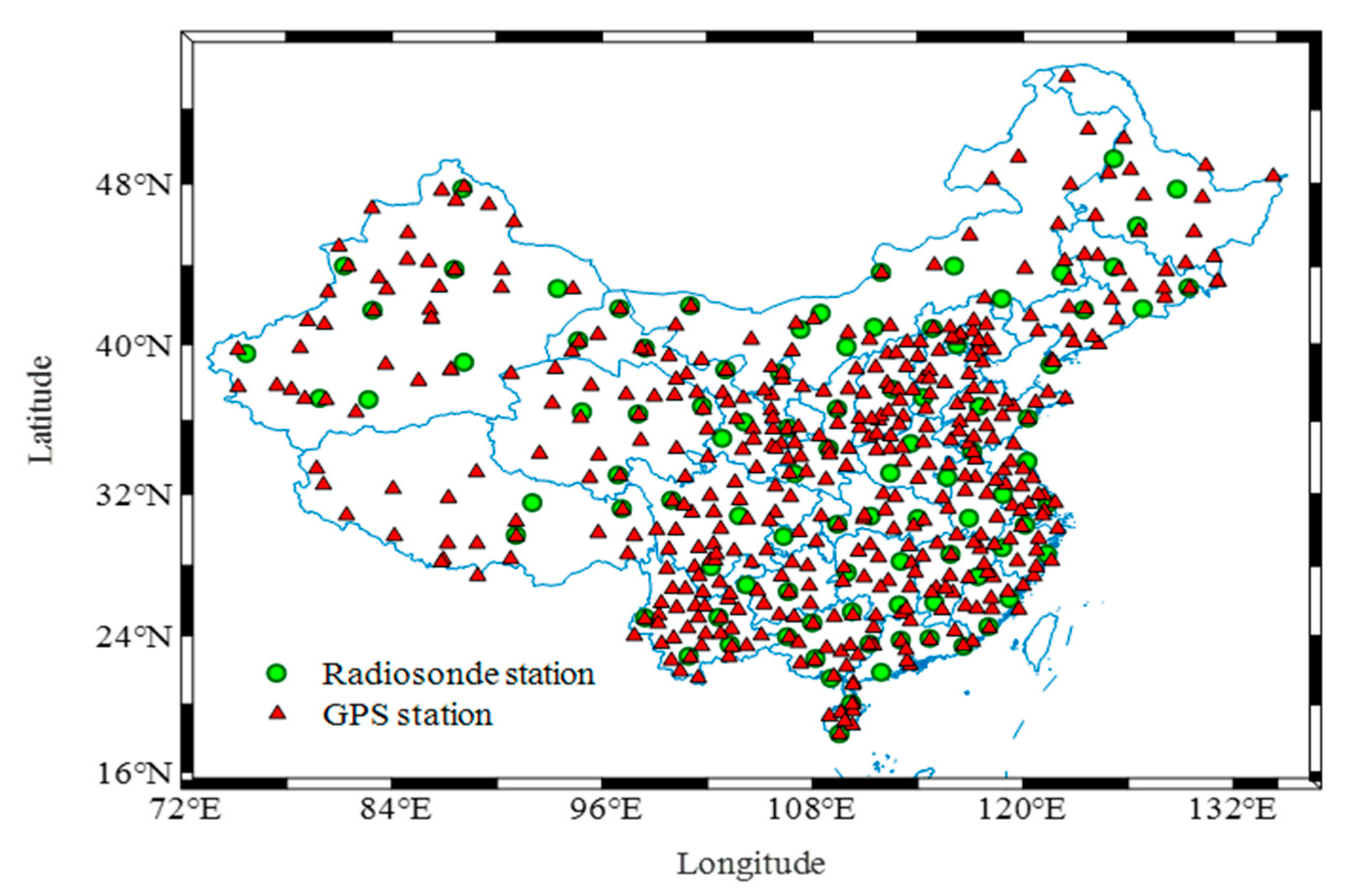
2.1. Observation Data

The infrastructure construction of national geodetic datum modernization in China was launched in 2012 and completed in 2017, which contained 210 GPS stations. A high-precision, dynamic, and unified modern surveying and mapping datum system was established to provide coordinate frame services, including data products, real-time positioning, processing and analysis, and other services [28]. Crustal Movement Observation Network of China (CMONC) was established in 2006 and completed in 2012, which contained 360 GPS stations [29,30]. The National Geomatics Center of China (NGCC) provided the hourly ZTD data and 1-h measured temperature and atmospheric pressure data at these GPS stations from 2011 to 2019. We used BERNESE 5.2 software [31] to process the raw data, including the implementation of daily solutions and adjustments [32].

The Integrated Global Radiosonde Archive (IGRA) has released radiosonde and pilot balloon observations with more than 2700 stations around the world since 1905, including air pressure, temperature, geopotential height, and relative humidity (ftp://ftp.ncdc.noaa.gov/pub/data/igra, accessed on 24 January 2021), whose temporal resolution is 12 h. We used IGRA-released radiosonde profiles in China from 2011 to 2019 to calculate the T_m at each radiosonde station. Figure 1 shows all the used GPS stations and radiosonde stations.

2.2. Establishment of Site-Specific Piecewise-Linear T_m-T_s Relationship

T_m is related to the temperature and vapor pressure at different altitudes in the atmosphere, which can be obtained from the IGRA. The method to calculating the 12-h T_m can be expressed as [13]:

$$T_m=\frac{{\int }_{z_0}^{+\infty }\left(\frac{e}{T}\right)dz}{{\int }_{z_0}^{+\infty }\left(\frac{e}{T^2}\right)dz}\approx \frac{{\sum }_{i=1}^N\left(\frac{e_i}{T_i}\right)\mathsf{\Delta }{z}_i}{{\sum }_{i=1}^N\left(\frac{e_i}{T_i^2}\right)\mathsf{\Delta }{z}_i}$$

(1)

where e (hPa) refers to the water vapor pressure, T (K) is the corresponding temperature, and Z (m) denotes the starting height of integration. $\mathsf{\Delta }{z}_i$ (m) denotes the altitude of the ith atmospheric layer, $N$ denotes the number of the atmospheric layer, $e_i$ (hPa) denotes the water vapor pressure of ith atmospheric layer, and $T_i$ (K) denotes the temperature of ith atmospheric layer. We converted the geopotential height into the geoid height in the calculation process.

The empirical formula based on the long-term radiosonde data in the study area and the linear relationship between surface temperature T_s and T_m can be established by a regression analysis as:

$$T_m=a·T_s+b$$

(2)

where $a$ and $b$ are the linear regression equation parameters.

The T_m variation has a significant annual variation. In some studies, the half-year variations and the daily variations are also considered when building the model. In order to get the time-varying characteristics of the T_m-T_s coefficient, a piecewise-linear least squares fitting is performed for each radiosonde station for one month.

2.3. PWV from Site-Specific Piecewise-Linear T_m-T_s Relationship

Three hundred and seventy-seven GPS stations were selected for estimating the PWV time series. Since the cubic spline method has a higher accuracy than the nearest-neighbor interpolation method and linear interpolation method, we used the cubic spline method to obtain the T_m-T_s model coefficients $a$ and $b$ at the GPS stations in the corresponding time period.

ZTD is the sum of Zenith Hydrostatic Delay (ZHD) and Zenith Wet Delay (ZWD), as

$$\mathrm{ZTD}=\mathrm{ZHD}+\mathrm{ZWD}$$

(3)

The Saastamoinent model has been widely used for ZHD computation [33], as

$$\mathrm{ZHD}=0.002277·\frac{P}{1-0.0026·cos (2\varphi )-0.00028·h_0}$$

(4)

where $P$ (hPa) denotes the ground pressure of the GPS station, $\varphi$ denotes the latitude of the GPS station, and $h_0$ (m) denotes the elevation of the GPS station.

The ZWD is caused by water vapor in the atmosphere under nonstatic equilibrium. Generally, empirical models and meteorological parameters at GPS station are used to obtain the ZHD, and then, the ZHD is deducted from the ZTD to obtain the ZWD.

$$\mathrm{ZWD}=\mathrm{ZTD}-\mathrm{ZHD}$$

(5)

The linear relationship between the ZWD and PWV can be expressed as [13]

$$\mathrm{PWV}=\mathsf{\Pi }·\mathrm{ZWD}$$

(6)

$$\mathsf{\Pi }= \frac{{10}^6}{{\rho }_w·\frac{R}{m_w}·\left[\frac{k_3}{T_m} + k_2 - \frac{m_w}{m_d}·k_1\right]}$$

(7)

where Π is the conversion factors between the ZWD and PWV; Π is a function of T_m; ${\rho }_w$ represents the density of the liquid water; $R$ is the universal gas constant and $R$ = 8314 Pa·m³·K⁻¹·kmol⁻¹; $m_w$ represents the molar mass of water vapor and $m_w$ = 18.02 kg·kmol⁻¹; $m_d$ represents the molar mass of the dry atmosphere and $m_d$ = 28.96 kg·kmol⁻¹; and $k_1, k_2,$ and $k_3$ are constants ($k_1$ = 77.604 ± 0.014 K/hPa, $k_2$ = 70. 4 K/hPa, and $k_3$= (3.776 ± 0.014) × 10⁵ K²/hPa) [13].

In general, approximately 6.7 mm of ZTD error will cause a PWV error of 1 mm. Hence, the ZTD with a Root Mean Square Error (RMSE) of greater than 6.7 mm are eliminated. In addition, ZTD data and meteorological parameters are missing at some stations in a few time periods. For sites with missing data for more than one year, they will not be used when analyzing the long-term changes. Then, Equations (3)–(6) were used for high-precision PWV estimations based on the site-specific piecewise-linear T_m-T_s relationship in China. Finally, the PWV time series derived from 377 GPS stations in China from 2011 to 2019 were obtained.

2.4. PWV from Radiosonde

The PWV at the radiosonde station is calculated as follows:

$$\mathrm{PWV}={{\displaystyle \int }}_0^{p_0}\frac{q}{{\rho }_{w}g}{d}_p$$

(8)

where $p$ (hPa) denotes the atmospheric pressure, $p_0$ (hPa) is the ground pressure at the GPS station, $q$(g·kg⁻¹) denotes the specific humidity, $g$ (m·s⁻²) is the acceleration of gravity, and ${\rho }_w$ (g·cm⁻³) refers to the density of the liquid water. By discretizing Equation (8), the integral equation of PWV from the ground to the top of the atmosphere is obtained as follows:

$$\mathrm{PWV}=-\frac{1}{g}{\displaystyle \sum }_{p_0}^{p}q\times p$$

(9)

2.5. Fitting Function of the PWV Time Series

Jin and Luo [34] analyzed the PWV series derived from 155 globally distributed GPS sites observations and found that most of the periods of the PWV series were 1 year, 0.5 years, 1 day, and 0.5 days. To fit the PWV time series of 377 GPS stations in China, we established the following equation:

$$\begin{gathered} \mathrm{PWV}=k_0+k_1·\cos \left(\frac{DOY-c_1}{365.25}·2\mathsf{\pi }\right)+k_2·\cos \left(\frac{DOY-c_2}{365.25}·4\mathsf{\pi }\right)+k_3·\cos \left(\frac{HOD-c_3}{24}·2\mathsf{\pi }\right)+k_4 \\ ·\cos \left(\frac{HOD-c_4}{24}·4\mathsf{\pi }\right)+\epsilon \end{gathered}$$

(10)

where $k_0$ is a constant term; $k_1$, $k_2,k_3,k_4,c_1,c_2,c_3$, and $c_4$ are the amplitude and phase at the period (1 year, 0.5 years, 1 day, and 0.5 days); DOY is the day of year; HOD is the hour of day; and $\epsilon$ is the residual. The least square method was used to determine the unknown parameters in Equation (10) with the PWV time series.

3. Evaluation and Comparison

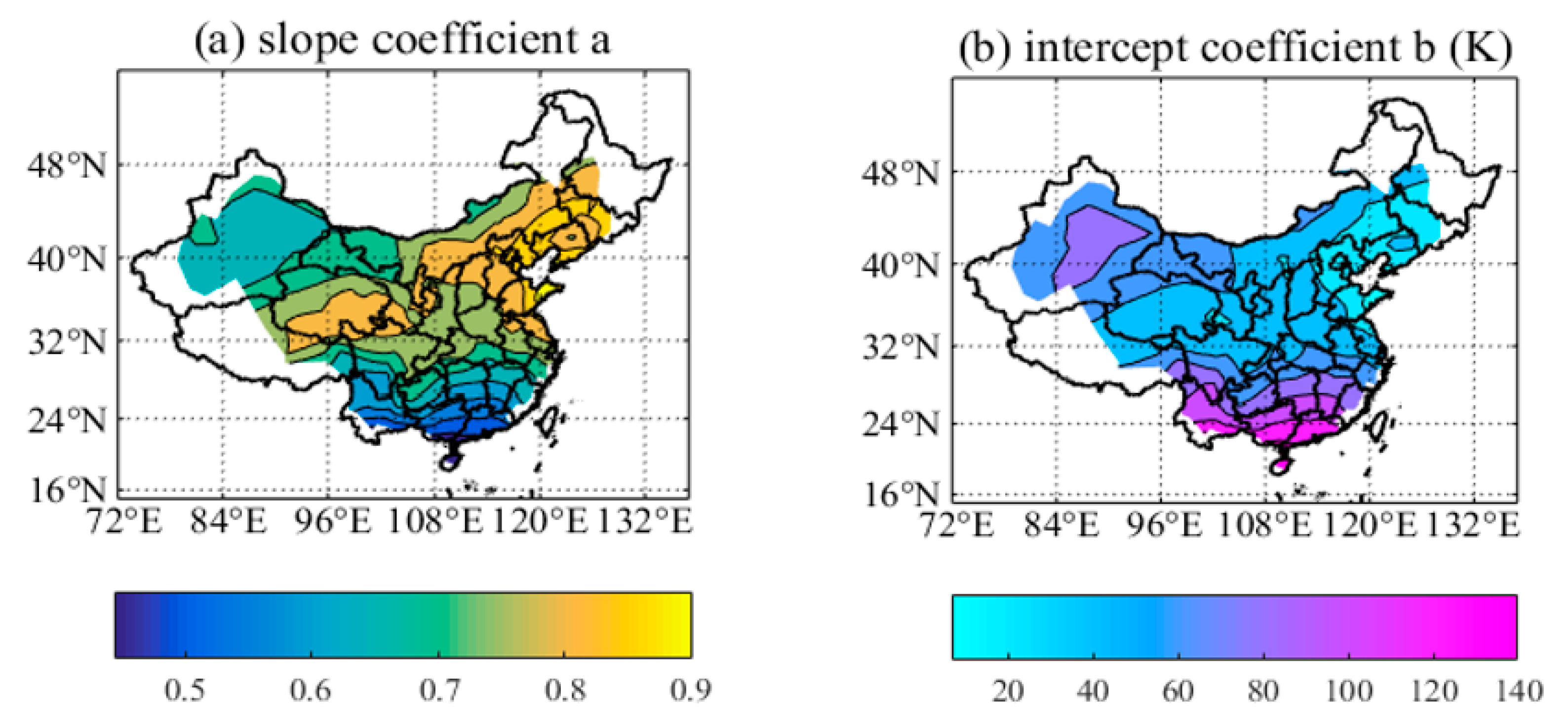
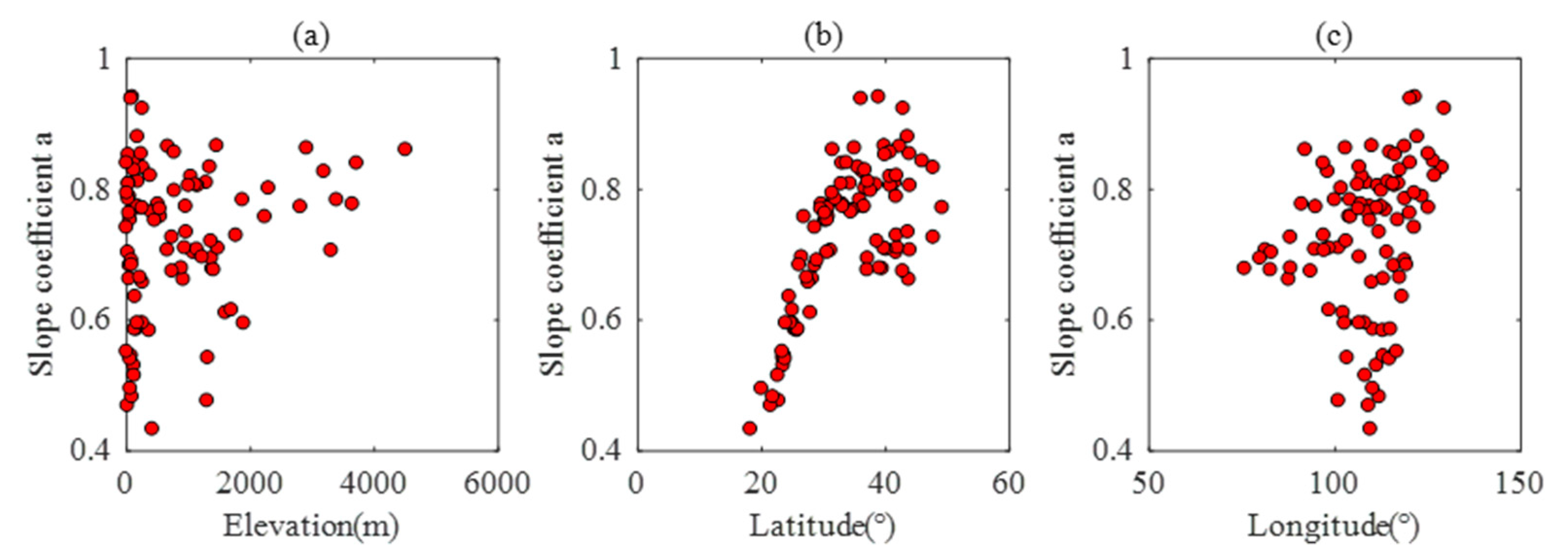
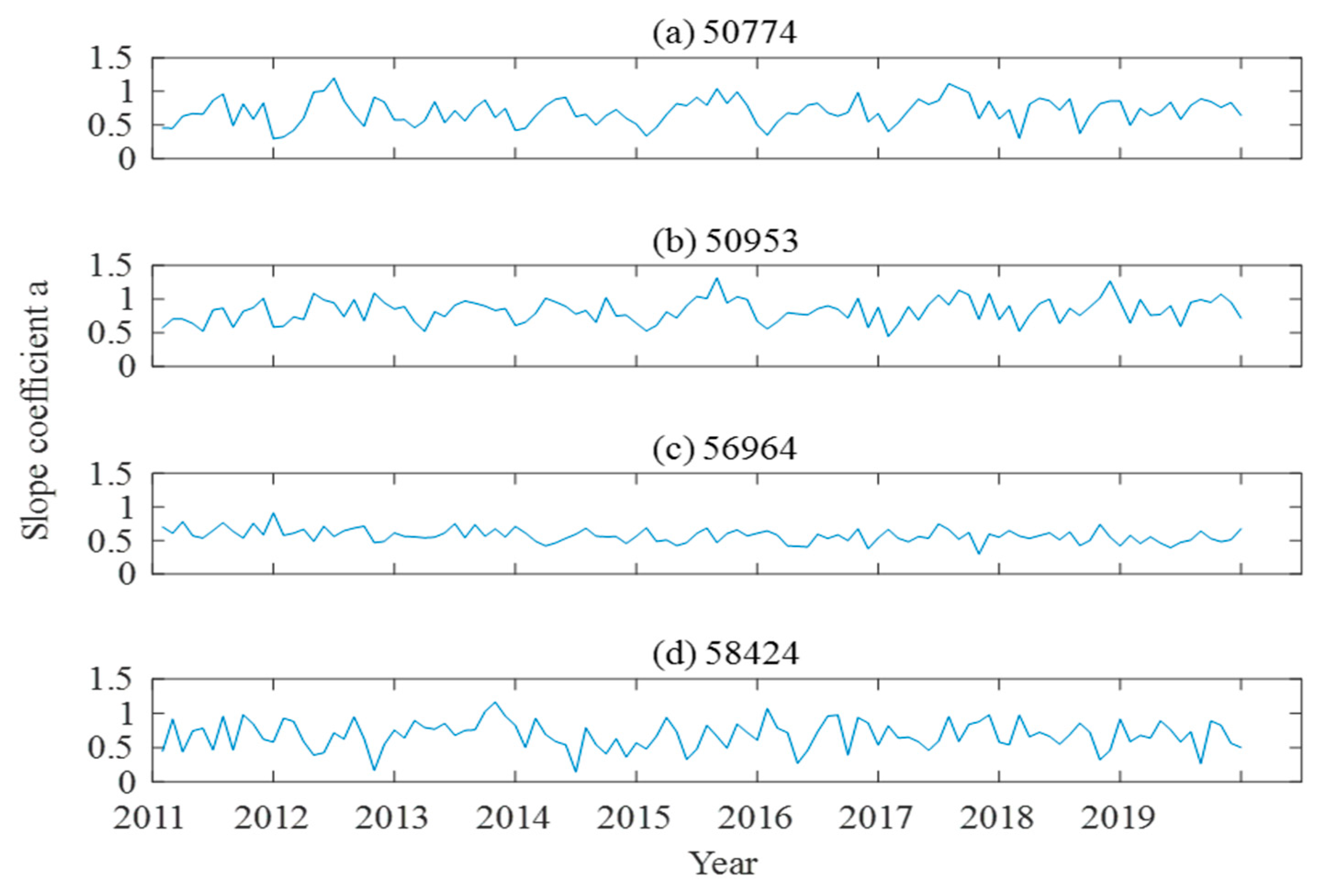
3.1. Spatial Distribution and Time-Varying Characteristics of the T_m-T_s Coefficient

Figure 2 shows the spatial distribution of the T_m-T_s relationship coefficients. The slope coefficient ranges from 0.5 to 0.7 in South China, around 0.7 in Northwest China, and about 0.8 in Central and Northeast China. As shown in the right panel, the intercept coefficient is from 80 to 140 in Southern China, about 60 in Central and Northwestern China, and approximately 20 in Northeastern China.

Figure 3 shows the distribution diagram of the slope coefficient with the elevation, latitude, and longitude. No evident correlation is found with the elevation and longitude, whereas there is strong positive correlation with the latitude, especially in low-latitude areas. Some studies have shown that when the same T_m-T_s coefficient is used at a global scale, it will cause different errors in the T_m of different latitudes [35,36]. Wang et al. found that the T_m derived from the Bevis T_m-T_s relationship has a cold bias in the tropics and subtropics and a warm bias in middle and high latitudes, and furthermore, the RMS was dominated by the mean bias rather than the random error. Therefore, the distribution of the T_m-T_s coefficients is mostly related to the latitude. The slope coefficient $a$ is generally less than 0.6 in low-latitude areas, which is consistent with the previous results of some global T_m-T_s models.

The monthly coefficients of the T_m-T_s model are obtained. The slope coefficients have obvious annual cycle at most stations. The time series of slope coefficients at four radiosonde stations are randomly selected and shown in Figure 4. The information of the four stations is shown in

Table 1. Information about the 4 stations used in Figure 4.

Name	Number	Latitude (°)	Longitude (°)	Height (m)
YICHUN	50,774	47.72	128.83	264.8
HARBIN	50,953	45.93	126.57	118.3
SIMAO	56,964	22.77	100.98	1303.0
ANQING	58,424	30.62	116.97	62.0

. The slope coefficients of the T_m-T_s model vary greatly with the time, from about 0.5–1. The regression slope and its changing tendency are smaller at the SIMAO station, which is due to the lower latitude.

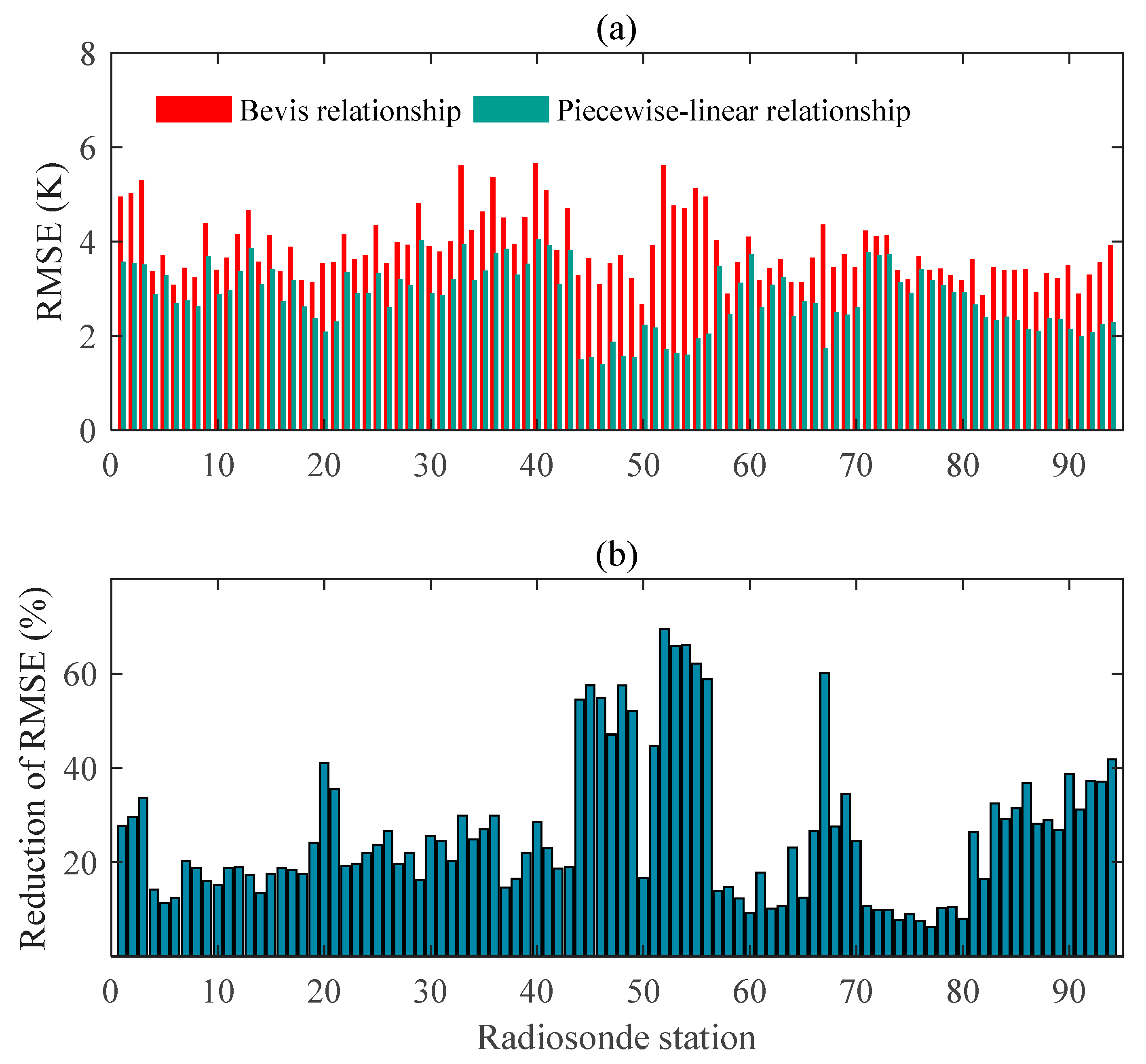
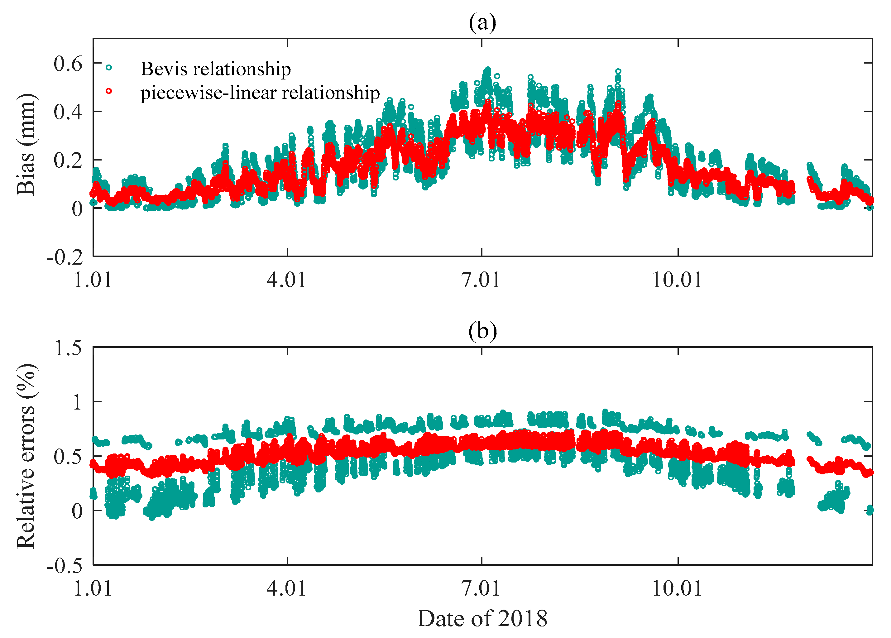
3.2. Comparison with Bevis T_m-T_s Relationship

We calculated the root mean square error (RMSE) (in unit of K) and accuracy improvement (%) of T_m for 94 radiosonde station, which are shown in Figure 5. Compared with the Bevis model, the site-specific piecewise-linear model has a significant improvement in the regression accuracy at most stations due to the consideration of the temporal and spatial distributions of the T_m-T_s conversion coefficient. According to the statistics, the T_m accuracy with 86 radiosonde stations is increased by more than 10% and by more than 20% with 52 radiosonde stations, and the lowest is increased by 6% (station 58457, 30.23° N, 120.17° E), and the highest is increased by 69% (station 56691, 26.87° N, 104.28° E).

Figure 6 shows the RMSE distribution of the Bevis model and the site-specific piecewise-linear model. As we can see, compared with the Bevis model, the single-station piecewise-linear model has a greater accuracy improvement in the southern, southwest, and northeastern regions by more than 30%. The increase in the central and northwestern regions is relatively small and approximately 15%.

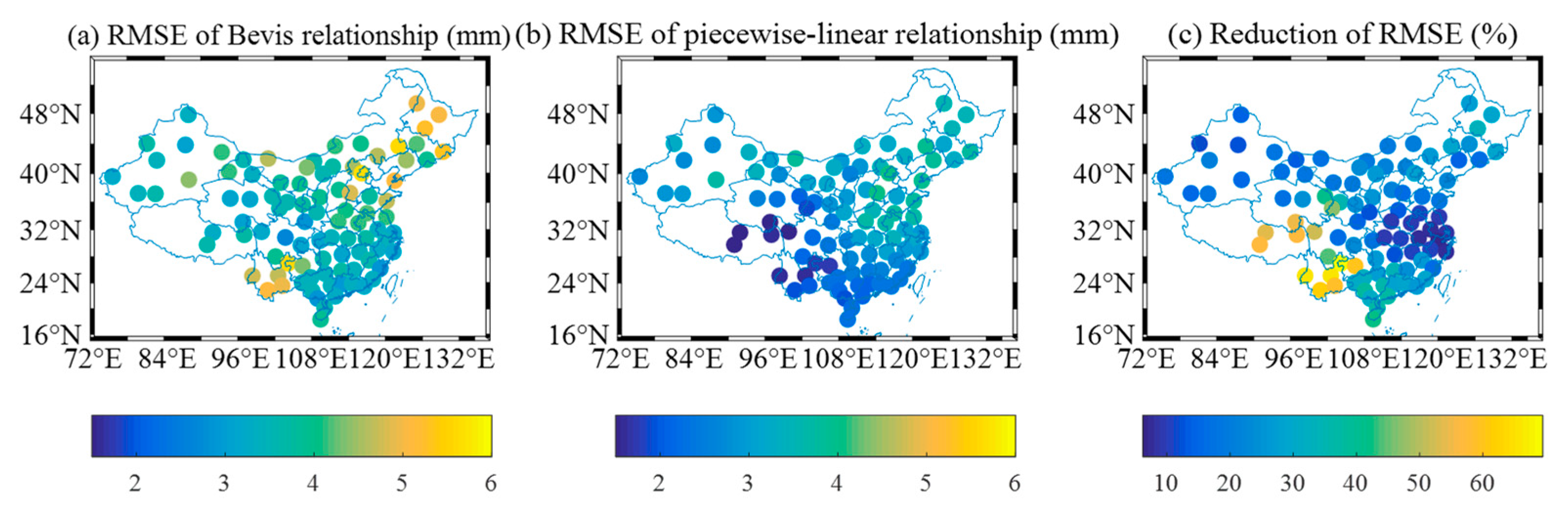
3.3. Comparison with GPS-Derived PWV and Radiosonde PWV

The selected GPS stations are closer to the radiosonde, in which the horizontal distance is less than 10 km and the elevation difference is less than 100 m. The water vapor obtained by the integral of the radiosonde profile data was used to evaluate the ground-based GPS PWV based on the Bevis model and the site-specific piecewise-linear T_m-T_s model. We calculated the deviation bias (in unit of mm) and relative errors. For example, Figure 7 shows the results at GXHC station in 2018. The accuracy of the PWV is better based on the site-specific piecewise-linear T_m-T_s relationship when compared to the Bevis’s model.

The distribution of water vapor in the atmosphere is not uniform. Thus, the ground-based GPS water vapor can get the average distribution of water vapor in each satellite signal direction. In addition, the layered meteorological parameter data of the radiosonde is not strictly vertical. These factors will bring errors into the PWV results. However, it still can be seen that the accuracy of the PWV is significantly improved based on site-specific piecewise-linear T_m-T_s relationship, especially when there are more atmospheric water vapors in the summer.

4. Variations Characteristics of GNSS PWV

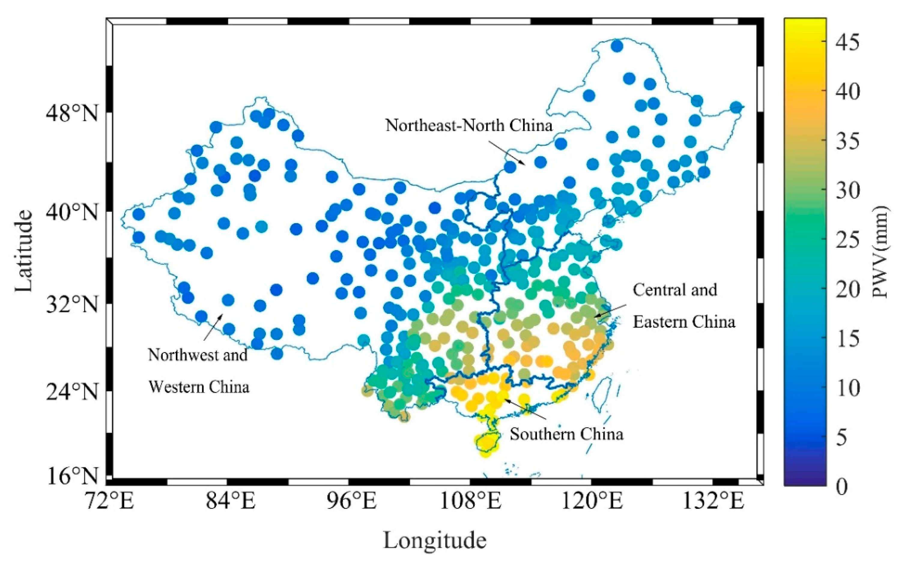
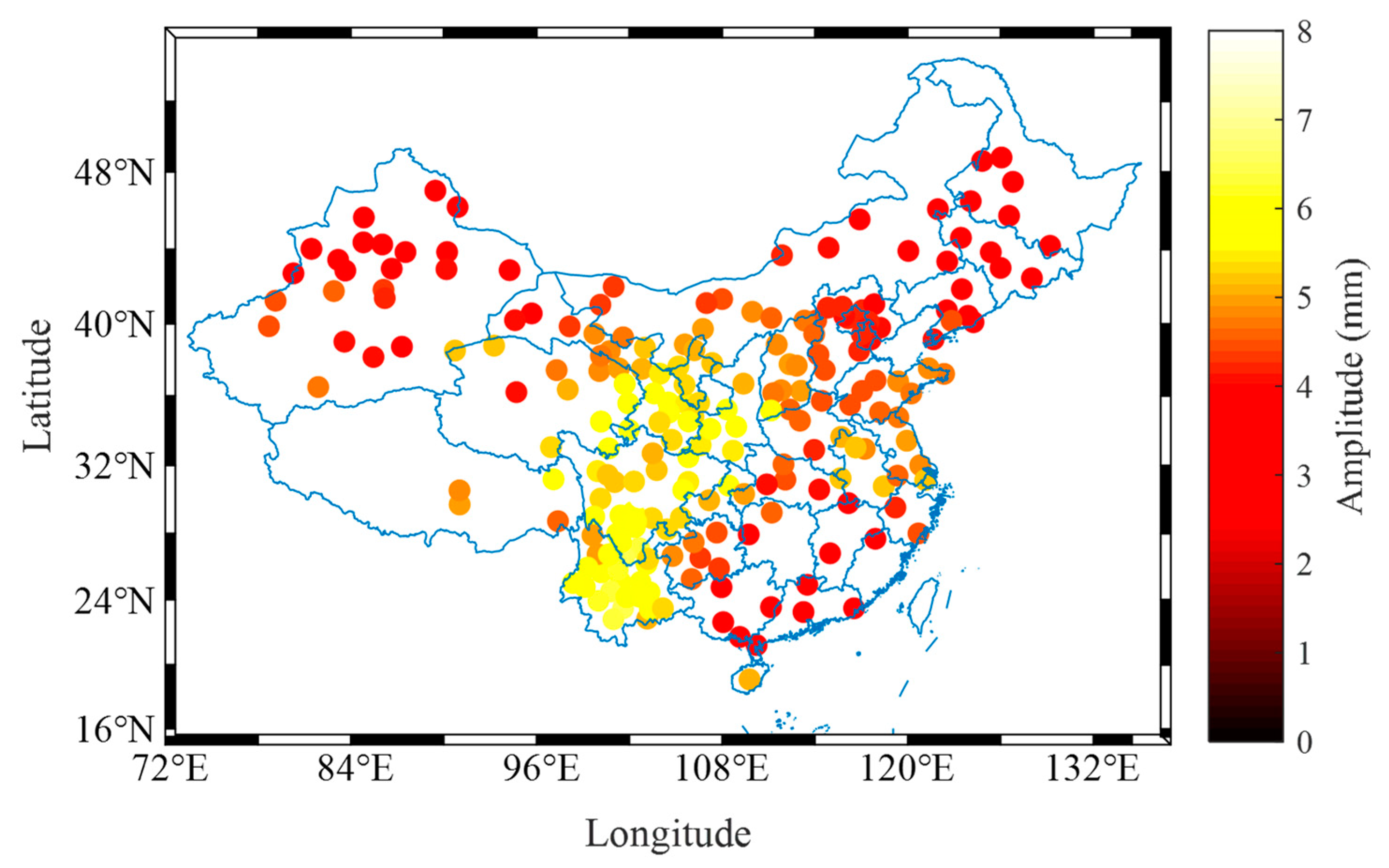
4.1. Spatial Distribution of PWV in China

The annual averaged PWV at all GPS stations from 2011 to 2019 in China range from 0 to 48 mm. As shown in Figure 8, the annual averaged PWV in Central-Eastern China and Southern China are relatively high, reaching above 25 mm, while the annual averaged PWV in Northwest, Northeast, and Northern China regions are lower, below 15 mm. Southeast China has a low latitude and is close to the East China Sea and the South China Sea, which are subject to subtropical monsoons. Monsoons transport water vapor from the sea to these areas, resulting in the higher annual averaged PWV [37]. Northwest China has a relatively high latitude and is an inland region with a temperate continental climate, so the annual averaged PWV is lower.

The GPS stations are divided into four regions: the eastern central region (24.5°–37° N, 105°–123° E), the southern region (19°–24. 5° N, 105°–120° E), the northwestern region (42°–49° N, 80°–90° E), and the northeastern region (37°–50° N, 110°–130° E). Figure 9 shows the nine-year daily averaged PWV of these four regions. The variation characteristics of the PWV in each region are consistent throughout the year, with the peaks in June and July and the droughts in January and December. Among them, the peak in Southern China appeared the earliest, which was affected by the south-to-north monsoon. Atmospheric circulation transported the water vapor to the Yangtze River Basin and then continued to transport it to other regions [38].

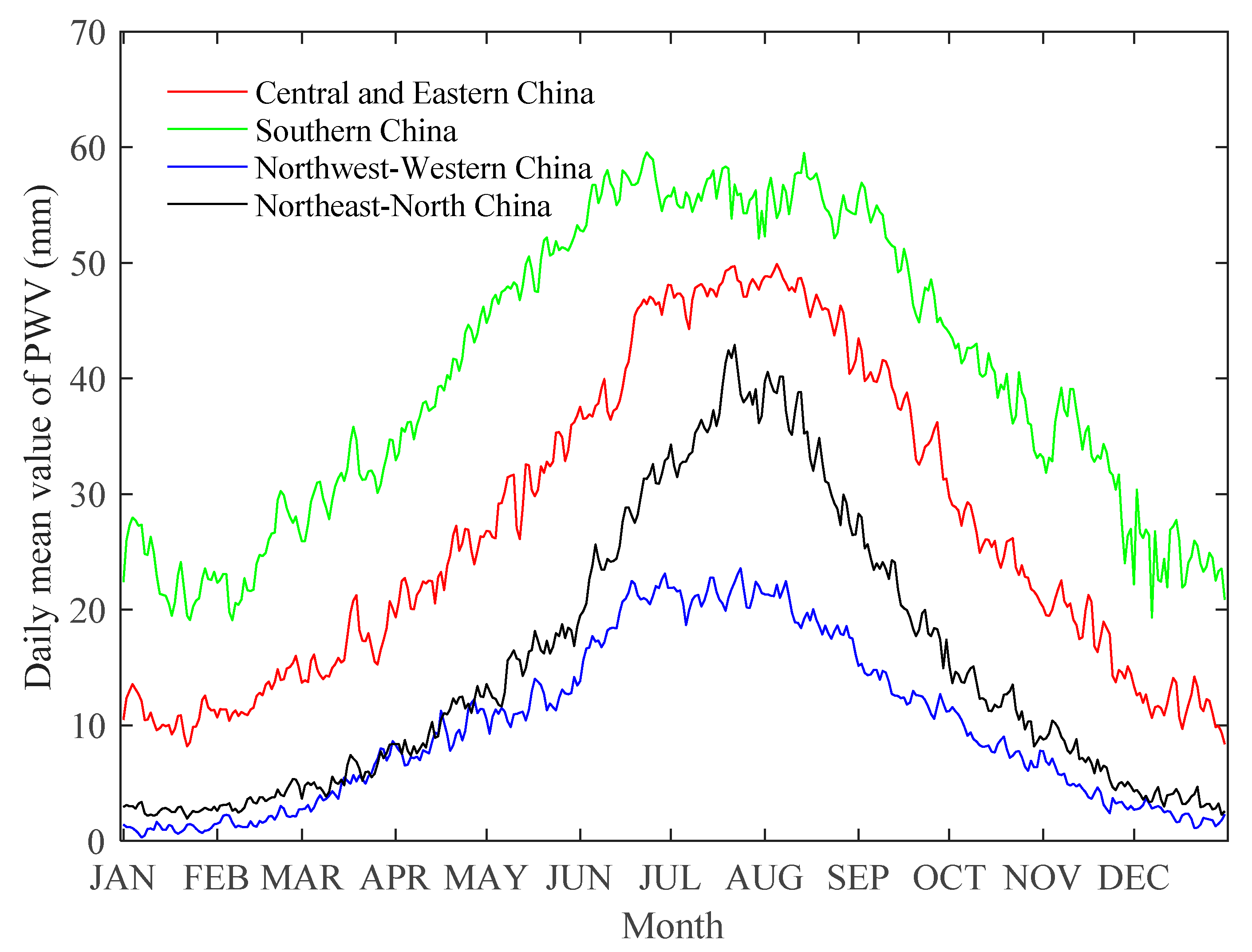
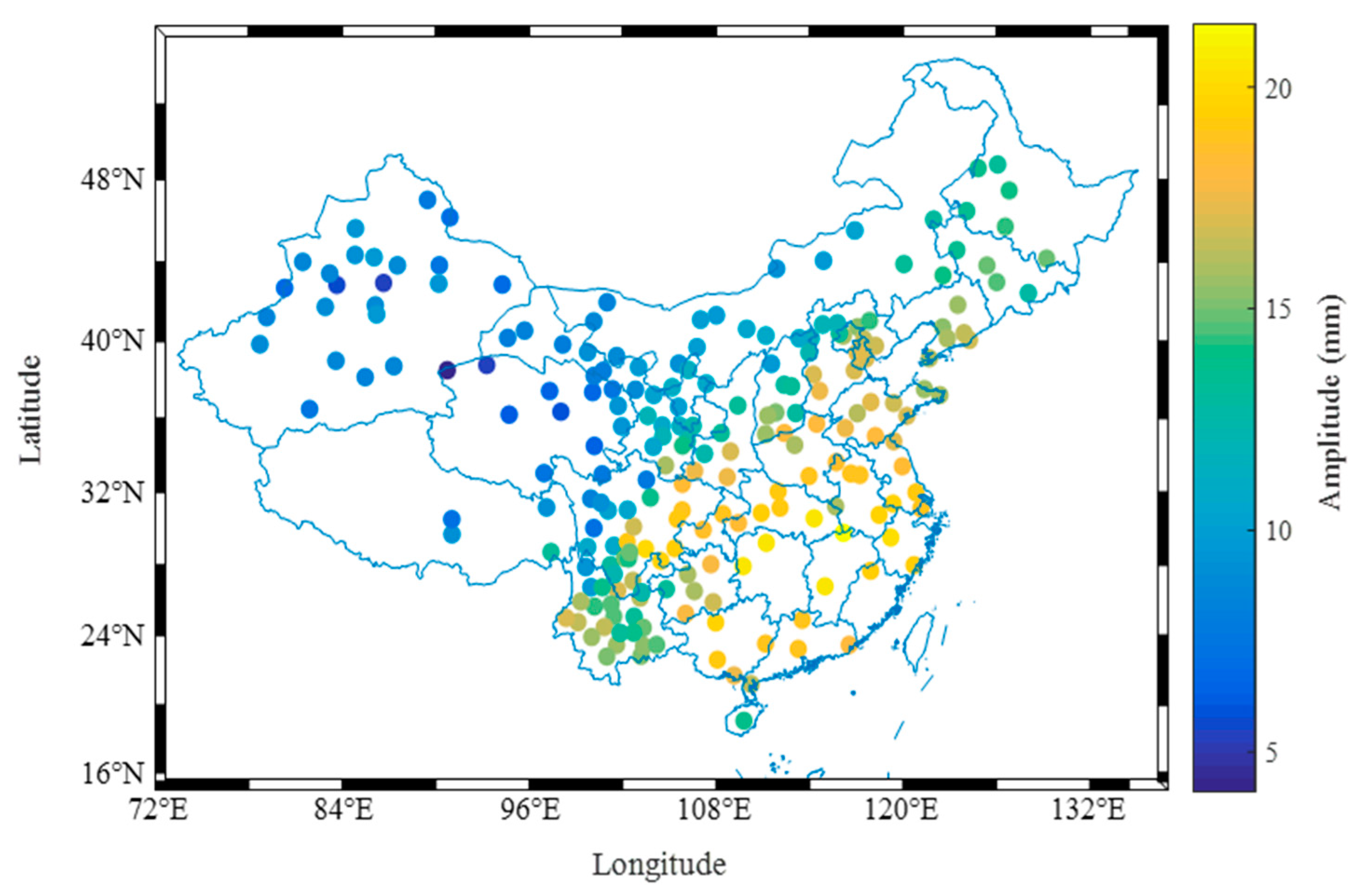
4.2. Seasonal Variations of PWV in China

Figure 10 and Figure 11 show the annual and semiannual PWV variation amplitudes at 377 GPS sites. The spatial distribution of the annual PWV variations is similar to the annual average distribution of the PWV. Central China, Southern China, and the southeast coastal areas have higher annual PWV variation amplitudes, reaching about 15 mm, while the annual cycle amplitude in Northwest China is lower, below 10 mm. The semiannual PWV variation amplitudes are relatively small, about 3–9 mm. Among them, the semiannual PWV variation amplitudes are the highest in Central China and Southwest China, reaching above 6 mm, while the semiannual PWV variation amplitudes in Southern China and Northwestern China are lower, below 5 mm.

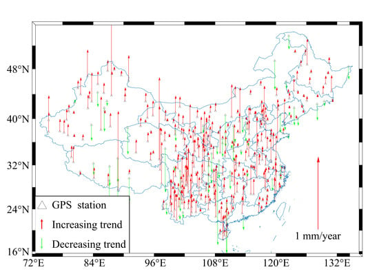
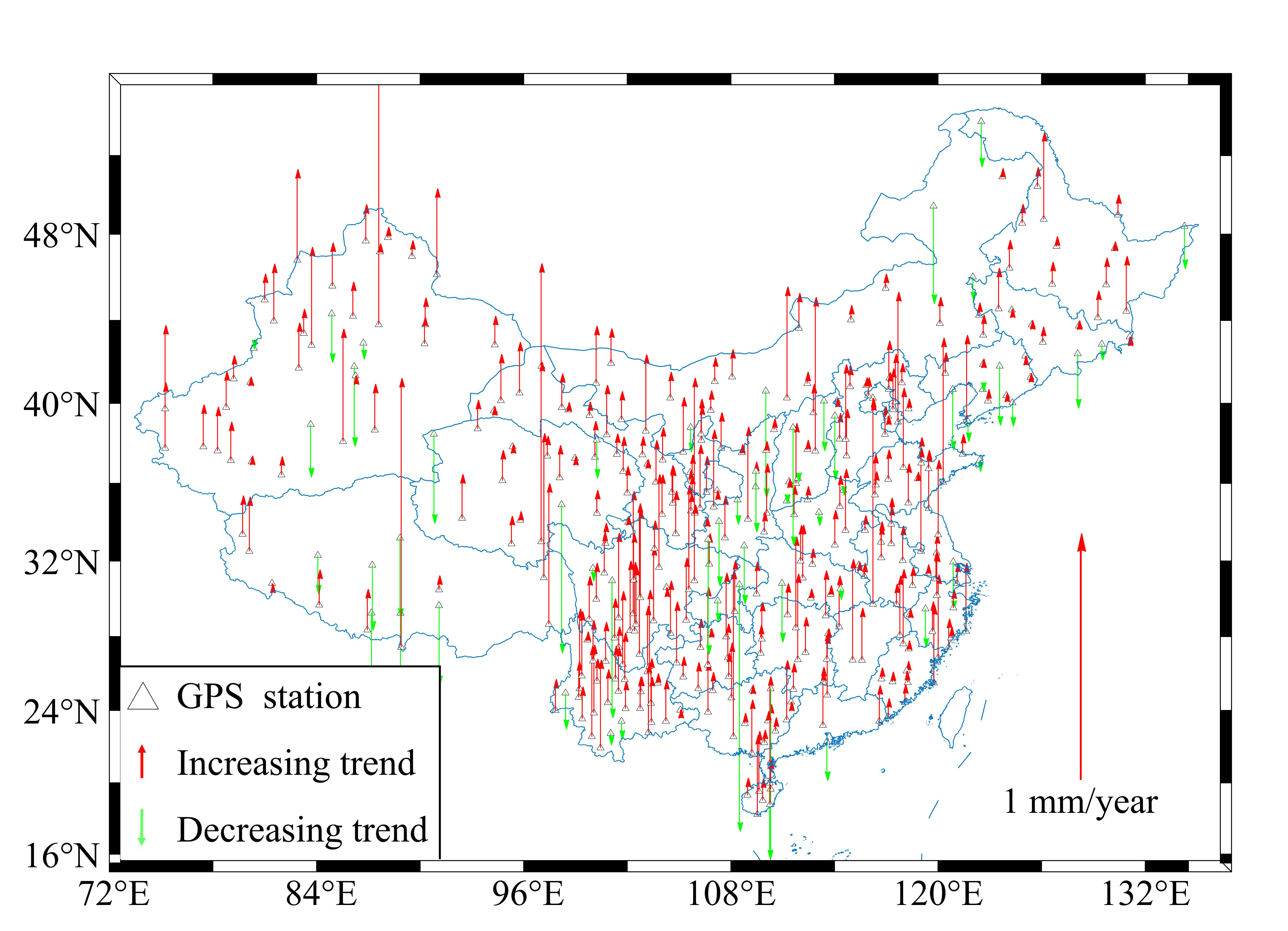
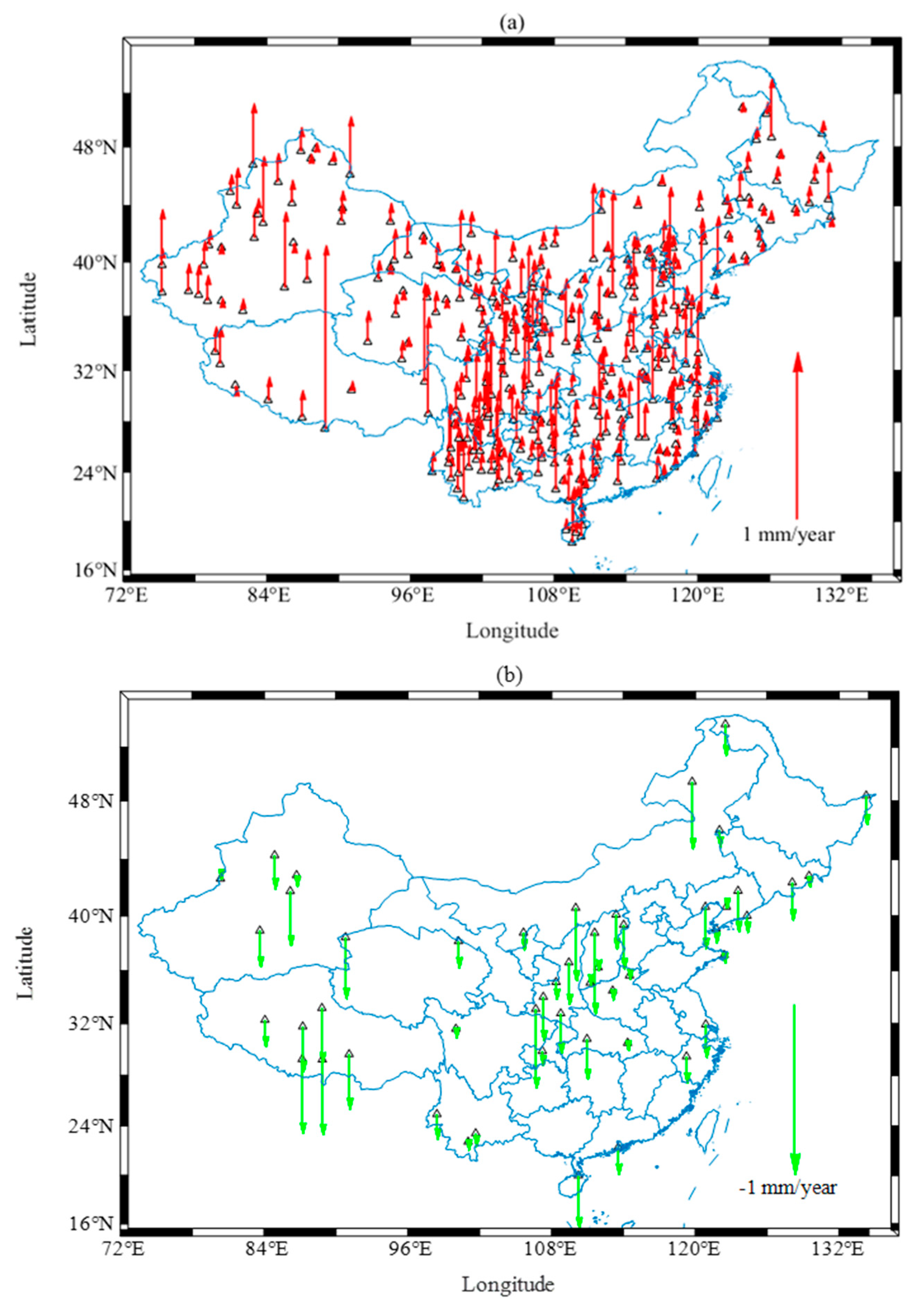
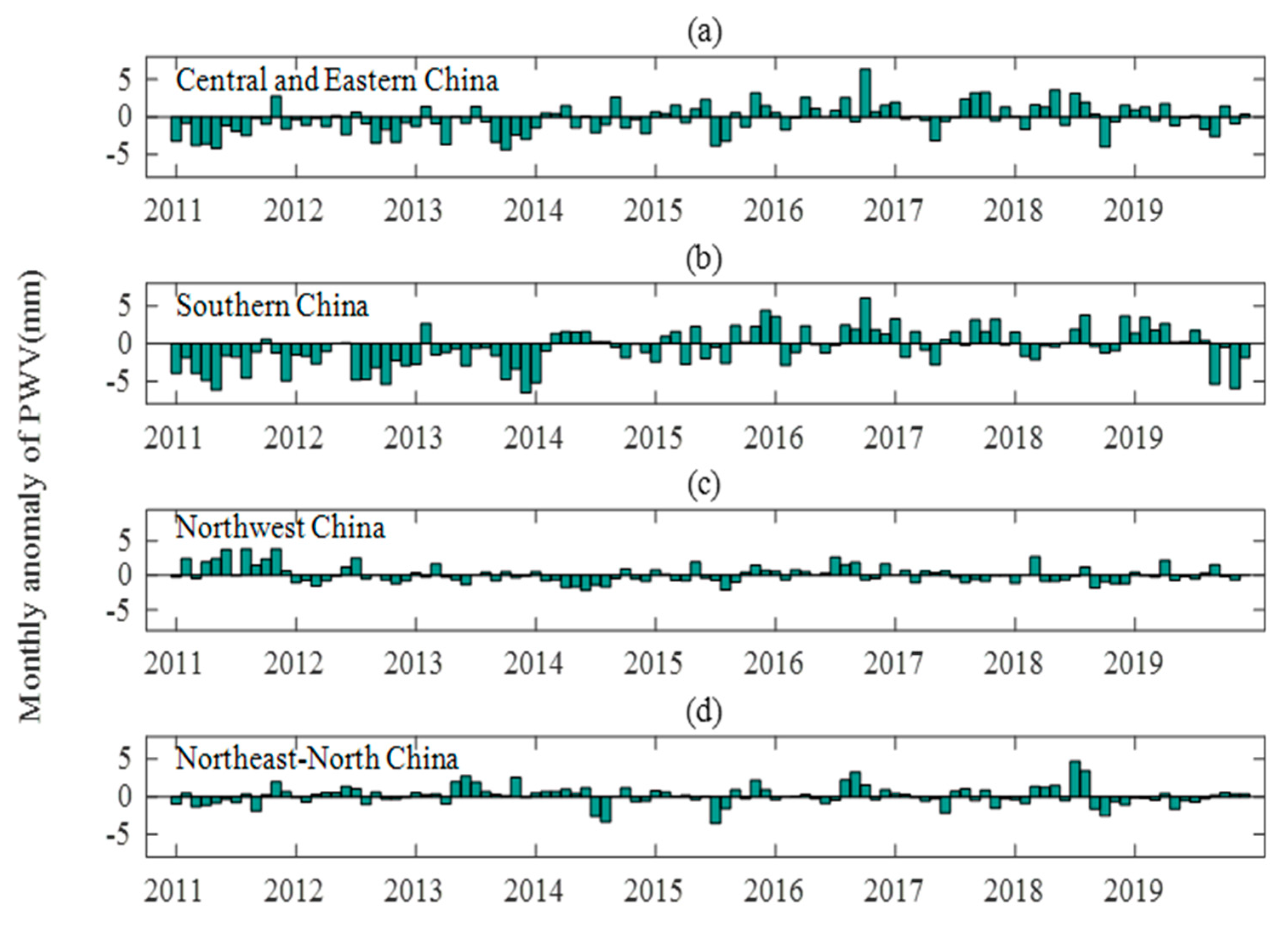
4.3. Long-Term Variation Trend of PWV in China

Figure 12 shows the long-term variation trends of the PWV (mm/year) of all GPS stations from 2011 to 2019. It can be seen that the PWV has been increasing in most parts of China, while the PWV in Northeast China shows a downward trend. To understand the variations of the PWV in more detail, a monthly anomaly of the PWV is obtained by subtracting the monthly averaged PWV of every month from the mean value of the monthly averaged nine-year PWV in each region, which can be seen in Figure 13. The monthly anomaly of the PWV was mainly negative before 2015 and then turned negative. The PWV in Northwest China, Northeast China, and Northern China were relatively stable, and the monthly mean value changed little, which was related to the dry inland climate.

5. Discussion

Most of the published T_m models that considered the temporal and spatial distributions of the relationship between the T_m and meteorological measurements have been empirical models on a global scale. Their accuracy remains to be verified in a specific area and a period of time. Here, we estimated the monthly coefficients at each station, and

Table 2. Statistics of the T_m estimates for different models.

Statistics	Bevis	TVGG	NN-I	Piecewise Linear
Bias (K)	−0.74	−1.25	0.03	0.00
RMS (K)	4.58	3.84	3.62	3.38

shows the comparison between the piecewise-linear model and two recently published representative models: the time-varying global-gridded T_s–T_m model (TVGG) and neural network-based T_m model (NN). We tested our model with radiosonde data from 2011 to 2019, and the results showed that our model has the best accuracy.

The spatial distribution characteristics of the PWV are consistent with other studies in different years [39,40]. There are bimodal characteristics of the PWV in Southern China, and the formation mechanism of the bimodal characteristics remains to be further studied. The past results of some studies in China indicated that the PWV showed a downward trend from 1995 to 2012 [41,42,43], while the trends of this article are upward from 2011 to 2019. Most PWV in Central and Eastern China and Southern China show an upward trend and some PWV in North China is downward from 2011 to 2019. The monthly averaged PWV increased significantly in 2015, which was affected by the El Niño.

6. Conclusions

In this study, we analyzed the temporal and spatial distribution characteristics of the coefficients of the linear T_m-T_s model and showed that the distribution of T_m-T_s coefficients is mainly related to the latitude. The T_m-T_s conversion coefficient changes with the time and has an obvious annual cycle. Based on the spatial distribution and time-varying characteristics of the T_m-T_s coefficients, a site-specific piecewise-linear model was established. Compared with the Bevis model, this model reduced the T_m RMS by more than 20% for the most of the tested radiosondes. The accuracy of GPS PWV is better based on the site-specific piecewise-linear T_m-T_s relationship when compared to the Bevis model. Furthermore, the PWV time series at 377 GNSS stations were further obtained and analyzed from the GPS observations and meteorological data from 2011 to 2019. The results showed that the average PWV in Central and Eastern China and Southern China is higher, reaching more than 25 mm, while the average value is lower and below 15 mm in Northwest China, Northeast China, and North China. The PWV is increasing in most parts of China, while some PWV in North China show a downward trend.

References

1. Philipona, R.; Dürr, B.; Ohmura, A.; Ruckstuhl, C. Anthropogenic greenhouse forcing and strong water vapor feedback increase temperature in Europe. Geophys. Res. Lett. 2005, 32. [Google Scholar] [CrossRef]
2. Gendt, G.; Dick, G.; Reigber, C.; Tomassini, M.; Liu, Y.; Ramatschi, M. Near real time GPS water vapor monitoring for numerical weather prediction in Germany. J. Meteorol. Soc. Jpn. Ser. II 2004, 82, 361–370. [Google Scholar] [CrossRef] [Green Version]
3. Boutiouta, S.; Lahcene, A. Preliminary study of GNSS meteorology techniques in Algeria. Int. J. Remote Sens. 2013, 34, 5105–5118. [Google Scholar] [CrossRef]
4. Sapucci, L.F. Evaluation of modeling water-vapor-weighted mean tropospheric temperature for GNSS-integrated water vapor estimates in Brazil. J. Appl. Meteorol. Climatol. 2014, 53, 715–730. [Google Scholar] [CrossRef]
5. Ning, T.; Wickert, J.; Deng, Z.; Heise, S.; Dick, G.; Vey, S.; Schöne, T. Homogenized time series of the atmospheric water vapor content obtained from the GNSS reprocessed data. J. Clim. 2016, 29, 2443–2456. [Google Scholar] [CrossRef]
6. Jin, S.; Su, K. PPP models and performances from single-to quad-frequency BDS observations. Satell. Navig. 2020, 1, 1–13. [Google Scholar] [CrossRef]
7. Jin, S.; Gao, C.; Li, J. Atmospheric sounding from Fengyun-3C GPS radio occultation observations: First results and validation. Adv. Meteorol. 2019, 1, 1–13. [Google Scholar] [CrossRef] [Green Version]
8. Jin, S.; Li, Z.; Cho, J. Integrated water vapor field and multiscale variations over China from GPS measurements. J. Appl. Meteorol. Climatol. 2008, 47, 3008–3015. [Google Scholar] [CrossRef]
9. Jones, J.; Guerova, G.; Douša, J.; Dick, G.; de Haan, S.; Pottiaux, E.; van Malderen, R. Advanced GNSS Tropospheric Products for Monitoring Severe Weather Events and Climate; COST Action ES1206 Final Action Dissemination Report; Springer: Berlin/Heidelberg, Germany, 2019; p. 563. [Google Scholar]
10. Steiner, A.; Kirchengast, G.; Foelsche, U.; Kornblueh, L.; Manzini, E.; Bengtsson, L. GNSS occultation sounding for climate monitoring. Phys. Chem. Earth Part A Solid Earth Geod. 2001, 26, 113–124. [Google Scholar] [CrossRef]
11. Smith, T.L.; Benjamin, S.G.; Gutman, S.I.; Sahm, S. Short-range forecast impact from assimilation of GPS-IPW observations into the Rapid Update Cycle. Mon. Weather Rev. 2007, 135, 2914–2930. [Google Scholar] [CrossRef]
12. Kourtidis, K.; Stathopoulos, S.; Georgoulias, A.; Alexandri, G.; Rapsomanikis, S. A study of the impact of synoptic weather conditions and water vapor on aerosol–cloud relationships over major urban clusters of China. Atmos. Chem. Phys. 2015, 15, 10955–10964. [Google Scholar] [CrossRef] [Green Version]
13. Bevis, M.; Businger, S.; Herring, T.A.; Rocken, C.; Anthes, R.A.; Ware, R.H. GPS meteorology: Remote sensing of atmospheric water vapor using the Global Positioning System. J. Geophys. Res. Atmos. 1992, 97, 15787–15801. [Google Scholar] [CrossRef]
14. Ross, R.J.; Rosenfeld, S. Estimating mean weighted temperature of the atmosphere for Global Positioning System applications. J. Geophys. Res. Atmos. 1997, 102, 21719–21730. [Google Scholar] [CrossRef] [Green Version]
15. Bokoye, A.I. Multisensor analysis of integrated atmospheric water vapor over Canada and Alaska. J. Geophys. Res. Atmos. 2003, 108, 4480. [Google Scholar] [CrossRef]
16. Emardson, T.R.; Derks, H.J. On the relation between the wet delay and the integrated precipitable water vapour in the European atmosphere. Meteorol. Appl. A J. Forecast. Pract. Appl. Train. Tech. Model. 2000, 7, 61–68. [Google Scholar] [CrossRef]
17. Wang, J.; Zhang, L.; Dai, A.; Hove, T.V.; Baelen, J.V. A near-global, 2-hourly data set of atmospheric precipitable water from ground-based GPS measurements. J. Geophys. Res. Atmos. 2007, 112, 112. [Google Scholar] [CrossRef] [Green Version]
18. Zhang, H.P.; Liu, J.N.; Zhu, W.Y.; Huang, C. Remote sensing of PWV using ground-based GPS data in Wuhan region. Prog. Astron. 2005, 23, 169–179. [Google Scholar]
19. Yao, Y.; Liu, J.; Zhang, B.; He, C. Nonlinear relationships between the surface temperature and the weighted mean temperature. Geomat. Inf. Sci. Wuhan Univ. 2015, 40, 112–116. [Google Scholar]
20. Jade, S.; Vijayan, M. GPS-based atmospheric precipitable water vapor estimation using meteorological parameters interpolated from NCEP global reanalysis data. J. Geophys. Res. Atmos. 2008, 113. [Google Scholar] [CrossRef] [Green Version]
21. Means, J.D.; Cayan, D. Precipitable water from GPS Zenith delays using North American regional reanalysis meteorology. J. Atmos. Ocean. Technol. 2013, 30, 485–495. [Google Scholar] [CrossRef]
22. Zhao, Q.; Yao, Y.; Yao, W.; Zhang, S. GNSS-derived PWV and comparison with radiosonde and ECMWF ERA-Interim data over mainland China. J. Atmos. Sol. Terr. Phys. 2019, 182, 85–92. [Google Scholar] [CrossRef]
23. Lu, C.; Li, X.; Cheng, J.; Dick, G.; Ge, M.; Wickert, J.; Schuh, H. Real-time tropospheric delay retrieval from multi-GNSS PPP ambiguity resolution: Validation with final troposphere products and a numerical weather model. Remote Sens. 2018, 10, 481. [Google Scholar] [CrossRef] [Green Version]
24. Abimbola, O.J.; Falaiye, O.A.; Omojola, J. Estimation of Precipitable Water Vapour in Nigeria Using NIGNET GNSS/GPS, NCEP-DOE Reanalysis II and Surface Meteorological Data. J. Phys. Sci. 2017, 28, 19. [Google Scholar] [CrossRef] [Green Version]
25. Zhang, H.; Yuan, Y.; Li, W.; Zhang, B.; Sensing, R. A real-time precipitable water vapor monitoring system using the national GNSS network of China: Method and preliminary results. IEEE J. Sel. Top. Appl. Earth Obs. 2019, 12, 1587–1598. [Google Scholar] [CrossRef]
26. Yao, Y.; Zhu, S.; Yue, S. A globally applicable, season-specific model for estimating the weighted mean temperature of the atmosphere. J. Geod. 2012, 86, 1125–1135. [Google Scholar] [CrossRef]
27. Yao, Y.; Hu, Y.; Yu, C.; Zhang, B.; Guo, J. An improved global zenith tropospheric delay model GZTD2 considering diurnal variations. Nonlinear Process. Geophys. 2016, 23, 127–136. [Google Scholar] [CrossRef] [Green Version]
28. Zhang, P.; Wu, J.; Sun, Z. Construction and Service of the National Geodetic Datum. Geomat. World 2018, 25, 39–41, 46. [Google Scholar]
29. Gan, W.; Li, Q.; Zhang, R.; Shi, H. Construction and Application of Tectonic and Environmental Observation Network of Mainland China. J. Eng. Stud. 2012, 4, 16–23. [Google Scholar]
30. Jin, S.; Park, P.-H.; Zhu, W. Micro-plate tectonics and kinematics in Northeast Asia inferred from a dense set of GPS observations. Earth Planet. Sci. Lett. 2007, 257, 486–496. [Google Scholar] [CrossRef]
31. Dach, R.; Lutz, S.; Walser, P.; Fridez, P. Bernese GNSS Software, version 5.2; Astronomical Institute, University of Bern: Bern, Switzerland, 2015. [Google Scholar]
32. Li, Z.; Wen, Y.; Zhang, P.; Liu, Y.; Zhang, Y. Joint Inversion of GPS, Leveling, and InSAR Data for The 2013 Lushan (China) Earthquake and Its Seismic Hazard Implications. Remote Sens. 2020, 12, 715. [Google Scholar] [CrossRef] [Green Version]
33. Saastamoinen, J. Contributions to the theory of atmospheric refraction. Bull. Géodésique 1973, 107, 13–34. [Google Scholar] [CrossRef]
34. Jin, S.; Luo, O. Variability and climatology of PWV from global 13-year GPS observations. IEEE Trans. Geosci. Remote Sens. 2009, 47, 1918–1924. [Google Scholar]
35. Liou, Y.-A.; Teng, Y.-T.; Van Hove, T.; Liljegren, J.C. Comparison of Precipitable Water Observations in the Near Tropics by GPS, Microwave Radiometer, and Radiosondes. J. Appl. Meteorol. 2001, 40, 5–15. [Google Scholar] [CrossRef]
36. Wang, J.; Zhang, L.; Dai, A. Global estimates of water-vapor-weighted mean temperature of the atmosphere for GPS applications. J. Geophys. Res. Atmos. 2005, 110. [Google Scholar] [CrossRef] [Green Version]
37. Guan, X.; Yang, L.; Zhang, Y.; Li, J. Spatial distribution, temporal variation, and transport characteristics of atmospheric water vapor over Central Asia and the arid region of China. Glob. Planet. Chang. 2019, 172, 159–178. [Google Scholar] [CrossRef]
38. Liu, Y.; Ding, Y. Analysis of the basic features of the onset of Asian summer monsoon. Acta Meteorol. Sin. 2007, 21, 511–526. [Google Scholar]
39. Zhao, Q.; Yang, P.; Yao, W.; Yao, Y. Hourly PWV Dataset Derived from GNSS Observations in China. Sensors 2020, 20, 231. [Google Scholar] [CrossRef] [PubMed] [Green Version]
40. Gui, K.; Che, H.; Chen, Q.; Zeng, Z.; Zheng, Y.; Long, Q.; Sun, T.; Liu, X.; Wang, Y.; Liao, T.; et al. Water vapor variation and the effect of aerosols in China. Atmos. Environ. 2017, 165, 322–335. [Google Scholar] [CrossRef]
41. Durre, I.; Williams, C.N.; And, X.Y.; Vose, R.S. Radiosonde-based trends in precipitable water over the Northern Hemisphere: An update. J. Geophys. Res. Atmos. 2009, 114. [Google Scholar] [CrossRef]
42. Wang, R. Characteristics of Water Vapor, Precipitation, Temperature and Humidity in Mainland China Based on IGRA and TRMM PR. Ph.D. Thesis, University of Science and Technology of China, Hefei, China, 2019. [Google Scholar]
43. Wong, M.S.; Jin, X.; Liu, Z.; Nichol, J.; Chan, P. Multi-sensors study of precipitable water vapour over mainland China. Int. J. Climatol. 2015, 35, 3146–3159. [Google Scholar] [CrossRef]
Figure 1. Distribution of GPS stations from the infrastructure construction of national geodetic datum modernization and Crustal Movement Observation Network of China (CMONC) in mainland China. The green circle is the radiosonde station, and the red triangle is the GPS station.
Remotesensing 13 01296 g001
Figure 2. Distribution of the Tm-Ts fitting coefficients a and b at each station by T m = a T s + b . (a) The slope coefficient a and (b) the intercept coefficient b .
Remotesensing 13 01296 g002
Figure 3. Distribution of the Tm-Ts model slope coefficient with the elevation (a), latitude (b), and longitude (c).
Remotesensing 13 01296 g003
Figure 4. Monthly slope coefficient of the Tm-Ts model from 2011 to 2019.
Remotesensing 13 01296 g004
Figure 5. RMSE (K) (a) and accuracy improvement of the Tm (b) calculated by the site-specific piecewise-linear and Bevis Tm-Ts relationship.
Remotesensing 13 01296 g005
Figure 6. RMSE (K) distribution of the Tm calculated by the site-specific piecewise-linear relationship (a), Bevis Tm-Ts relationship (b), and reduction of the RMSE (%) by the site-specific piecewise-linear Tm-Ts relationship (c).
Remotesensing 13 01296 g006
Figure 7. Bias (mm) (a) and relative error (%) (b) of the precipitable water vapor (PWV) calculated based on different Tm-Ts models at GXHC station in 2018. The blue dots are the PWV based on the Bevis model, and the red dots are the PWV based on the site-specific piecewise-linear model.
Remotesensing 13 01296 g007
Figure 8. Annual averaged PWV (mm) in China from 2011 to 2019.
Remotesensing 13 01296 g008
Figure 9. Nine-year averaged daily PWV (mm) in four regions of China from 2011 to 2019.
Remotesensing 13 01296 g009
Figure 10. Annual PWV variation amplitudes (mm) at 377 GPS sites.
Remotesensing 13 01296 g010
Figure 11. Semiannual PWV variation amplitudes (mm) at 377 GPS sites.
Remotesensing 13 01296 g011
Figure 12. Long-term variation trend of the PWV. The red upward arrows (a) stand for the increase of the PWV variation trend (mm/year), and the green downward arrows (b) represent the decrease of the PWV variation trend (mm/year).
Remotesensing 13 01296 g012
Figure 13. Monthly anomaly (mm) of the PWV in four regions of China.
Remotesensing 13 01296 g013