Article

Monitoring Dynamic Evolution of the Glacial Lakes by Using Time Series of Sentinel-1A SAR Images

1
Faculty of Geosciences and Environmental Engineering, Southwest Jiaotong University, Chengdu 611756, China
2
State-Province Joint Engineering Laboratory of Spatial Information Technology of High-Speed Rail Safety, Chengdu 611756, China
3
Institute of Mountain Hazards and Environment, Chinese Academy of Sciences, Chengdu 610041, China
*
Author to whom correspondence should be addressed.
Submission received: 16 February 2021 / Revised: 25 March 2021 / Accepted: 26 March 2021 / Published: 30 March 2021

Abstract

:
As an approach with great potential, the interpretation of space-borne synthetic aperture radar (SAR) images has been applied for monitoring the dynamic evolution of the glacial lakes in recent years. Considering unfavorable factors, such as inherent topography-induced effects and speckle noise in SAR images, it is challenging to accurately map and track the dynamic evolution of the glacial lakes by using multi-temporal SAR images. This paper presents an improved neighborhood-based ratio method utilizing a time series of SAR images to identify the boundaries of the glacial lakes and detect their spatiotemporal changes. The proposed method was applied to monitor the dynamic evolution of the two glacial lakes with periodic water discharge at the terminus of the Gongba Glacier in the southeastern Tibetan Plateau by utilizing 144 Sentinel-1A SAR images collected between October of 2014 and November of 2020. We first generated the reference intensity image (RII) by averaging all the SAR images collected when the water in the glacial lakes was wholly discharged, then calculated the neighborhood-based ratio between RII and each SAR intensity image, and finally identified the boundaries of the glacial lakes by a ratio threshold determined statistically. The time series of areas of the glacial lakes were estimated in this way, and the dates for water recharging and discharging were accordingly determined. The testing results showed that the water of the two glacial lakes began to be recharged in April and reached their peak in August and then remained stable dynamically until they began to shrink in October and were discharged entirely in February of the following year. We observed the expansion process with annual growth rates of 3.19% and 12.63% for these two glacial lakes, respectively, and monitored a glacial lake outburst flood event in July 2018. The validation by comparing with the results derived from Sentinel-2A/B optical images indicates that the accuracy for identifying the boundaries of the glacial lakes with Sentinel-1A SAR images can reach up to 96.49%. Generally, this contribution demonstrates the reliability and precision of SAR images to provide regular updates for the dynamic monitoring of glacial lakes.

Graphical Abstract

1. Introduction

Over the past decades, climate warming has exacerbated the melting of glaciers in most of High Mountain Asia [1,2,3,4]. The glaciers in the southeastern Tibetan Plateau and its vicinity have been observed with the most negative mass balances [3,4]. The continuous mass losses of glaciers are generally accompanied by the increase in the amount and the expansion in the area of glacial lakes [5,6], resulting in an increased risk of glacial lake outburst floods (GLOF) [7,8,9]. Monitoring the dynamic evolution of glacial lakes is essential for understanding the interactions between their spatiotemporal changes under climate warming and the risk assessment of related hazards.
Current and accurate mapping of the glacial lakes is the basis for monitoring dynamic evolution and further research. With the emergence of many earth observation satellites, such as the Landsat series and Sentinel-2 A/B constellation, remote sensing technology has been widely used for the inventory and dynamic monitoring of glacial lakes [6,7,8,10,11,12,13]. Some conventional methods, such as spectral classification [14] and spectral transformation methods [15,16], are widely applied to identify the water surface. To enhance water bodies from the adjacent objects, McFeeters (1996) proposed a normalized difference water index (NDWI) algorithm to monitor changes related to water content using green and near-infrared (NIR) wavelengths [17]. Many studies about NDWI have been developed and applied to investigate and inventory glacial lakes [11,18,19,20,21]. However, mapping glacial lakes based on optical remote sensing is susceptible to shadow effects because they are mostly situated in high mountain areas with complex terrains. Also, for areas frequently covered with heavy clouds in the warm season, like the southeast Tibetan Plateau dominated by the Indian and Bengal monsoons, the acquisition of available cloud-free optical images is severely restricted.
Synthetic aperture radar (SAR) represents an alternative to optical satellites for feature classification [22,23] and change detection [24,25] with the capability to collect data under all weather conditions without the restriction of clouds [26]. Since the smooth water surface will cause the incident SAR signal to be specularly reflected, the backscattered intensity in the SAR image corresponding to the water bodies is generally lower than their surroundings. Previous studies mostly used manual digitization or threshold segmentation to delineate the boundaries of glacial lakes [25,27,28,29,30]. However, due to the unique Range–Doppler imaging geometry of SAR images and the physical characteristics of radar waves, several issues may cause low-level amplitude in SAR images, such as incident angle, look direction, moisture on the surface, and the physical composition of the ground feature [26,31,32,33]. In other words, the pixels with low-level backscattered intensity in SAR images are not all matched to the water bodies, with the result that identification of glacial lakes directly based on the intensity values of SAR image may cause misclassification.
Some methods have been reported on change detection for SAR images. Most of them are designed for bitemporal SAR images, such as the neighborhood-based ratio (NR) approach [34,35] and logarithmic transformation ratio (Log-Ratio) method [36]. The main objective of these methods is to detect the changed targets from stable areas between two acquisitions instead of focusing on the mapping of ground objects. Additionally, SAR images are susceptible to speckle noise and physical characteristics of ground objects [26,37], resulting in redundancy and random discriminations. Although these methods have been widely used as indicators of change detection, there are rare studies on the application to extract the boundary and monitor the dynamic evolution for glacial lakes.
In this study, we developed an improved method based on the neighborhood-based ratio method to semi-automatically identify the boundaries of glacial lakes and detect their spatiotemporal changes. We selected two glacial lakes with periodic water discharge at the terminus of Gongba Glacier, southeast Tibetan Plateau, as the study site demonstrated the technique we developed, based on 144 Sentinel-1 C-band SAR images acquired from October 2014 to November 2020.

2. Study Area and Data Sources

2.1. General Information about the Study Area

The Gongba Glacier is located on the west slope of the Mount Gongga (29°35′45″N, 101°52′45″E, 7556 m), southeastern Tibetan Plateau [38,39,40], as shown in Figure 1a. Between the 17th and 19th centuries, the Gongba Glacier was divided into the Dagongba Glacier on the south side and the Xiaogongba Glacier on the north side [39]. According to the second glacial inventory data set of China [41], the Dagongba Glacier has a length of 10.6 km and an area of 19.1 km2 in 2009, and those for Xiaogongba Glacier are 6.46 km and 5.73 km2, respectively. The two glaciers are the typical debris-covered type, with the moraine extended from the terminus at 3900 m elevation to the foot of icefall at 4700 m elevation [42,43].
In recent years, a large number of supraglacial ponds and moraine-dammed lakes have been formed on the glacier tongue, of which the largest two are located at the terminus of Dagongba Glacier and Xiaogongba Glacier, labeled the Dagongba Glacial Lake (DGL) at 4100 m elevation and the Xiaogongba Glacial Lake (XGL) at 4130 m elevation, respectively, with a total area of more than 120,000 m2 (see Figure 1b). By the interpretation of satellite images, the water in both XGL and DGL is characterized by periodic recharging in the warm season and discharging in the cold season. According to our field survey in June and October 2018, the XGL and DGL are formed when the runoff at the glacier surface is obstructed and gathered by the terminal moraine deposits.

2.2. Data Sources

In this study, a total of 144 Sentinel-1A satellite ascending C band SAR images acquired between October 2014 to November 2020 were used for mapping the boundaries of glacial lakes and monitoring their dynamic evolution. All the downloaded SAR images are of the interferometric wide swath mode and the Level-1 single look complex data products with the spatial resolution of 13.96 m in azimuth direction and 2.33 m in range direction [44]. The Sentinel-1 A satellite acquired data covering the study area only in single-polarization (VV) mode between October 2014 and January 2017 (a total of 30 frames in this case) and acquired data using dual-polarization (VV+VH) mode since February 2017. Thus, for all the selected SAR images, the following processing using VV-polarization mode was uniformly performed. In addition to the SAR images, the Shuttle Radar Topography Mission (SRTM) digital elevation model (DEM) with a spatial resolution of approximately 30 m (1 arc-sec) was used for the co-registered processing of SAR images and subsequent projection conversion.
For validation purposes, 40 optical images acquired by the Sentinel-2 satellite from November 2016 to November 2020 were used for comparison and accuracy validation with the derived boundaries of glacial lakes based on SAR images. The Sentinel-2 is comprised of a constellation of two polar-orbiting satellites placed in the same sun-synchronous orbit that has the capacity of a high revisit period of 5 days to obtain multispectral remote sensing images with the resolution of 10 m [45]. However, considering that the acquisition of space-borne optical satellite images covering the Gongba Glacier is vulnerable to obstruction by heavy clouds, especially in summer, all selected optical images are filtered manually to ensure that the area of interest is under cloud-free conditions.

3. Methodology

Figure 2 shows the data processing flow chart of the proposed method. The main steps of the proposed approach include the generation of reference intensity image (RII), calculation of the neighborhood-based ratio, and the selection of a threshold for classification. In the following text, we will first describe the definition of the neighborhood-based ratio method and generation of RII and then discuss the effectiveness of the proposed method in the classification of glacial lakes (Section 3.1). Second, statistical analysis will be used to compute the threshold for automatic classification of time series of ratio maps (Section 3.2). Additionally, the boundaries extracted based on Sentinel-2 A/B satellite images are assumed to be the ground truth to validate the accuracy of the results derived from the proposed method (Section 3.3).

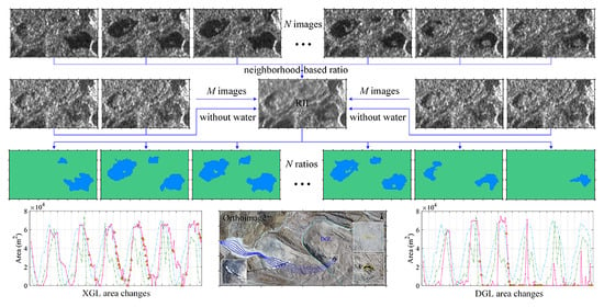
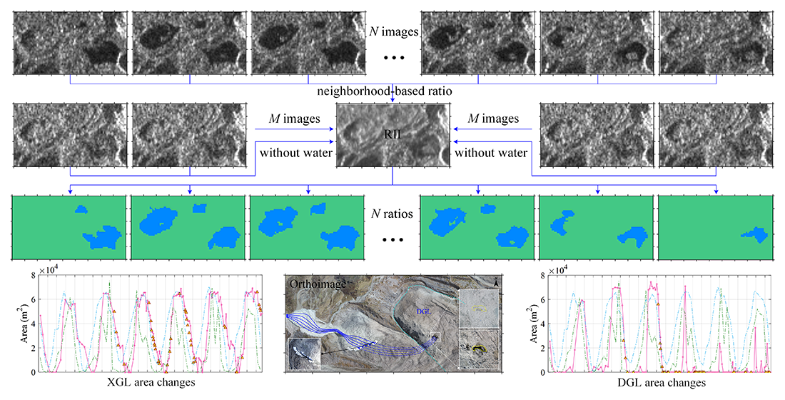
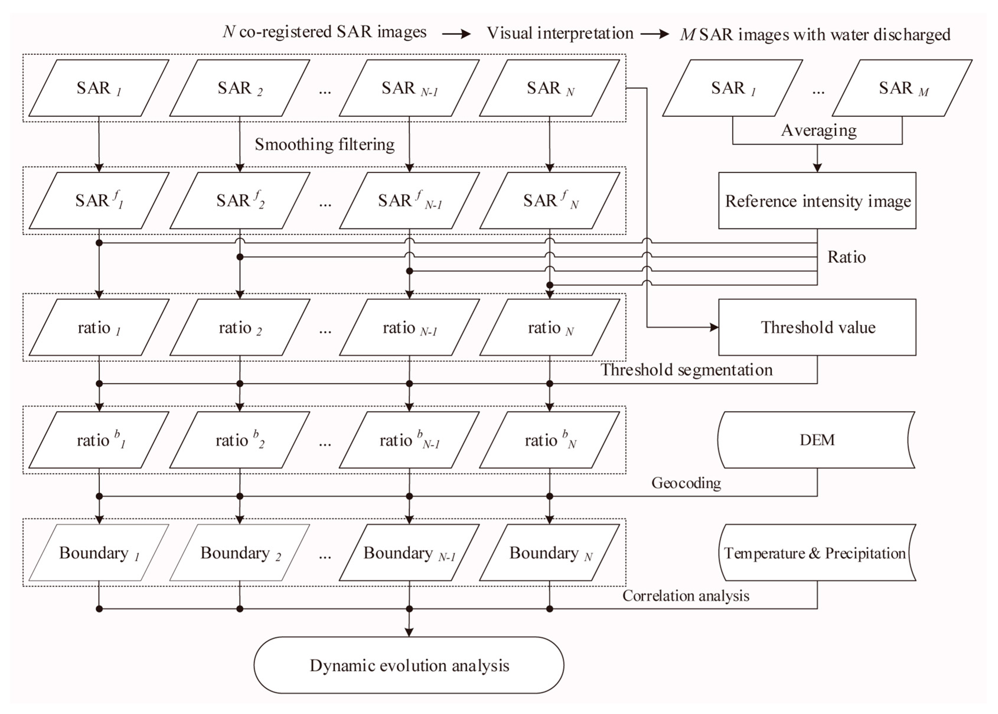
3.1. The Improved Neighborhood-based Ratio Method

For bitemporal SAR images of the same geographical area acquired at different dates, the normalized neighborhood-based ratio (NR) method can be defined as [34]:
NR ( I 1 / I 2 ) = 1 m i n ( μ 1 ( r , c ) μ 2 ( r , c ) , μ 2 ( r , c ) μ 1 ( r , c ) )
where I1 and I2 represent the two co-registered SAR images acquired on different dates; μ1(r,c)and μ2(r,c) denote the local mean intensity values in the defined window size and defined weighting function (e.g., linear weighting and Gaussian weighting) for the pixel position (r,c) in I1 and I2, respectively; and min denotes the minimum operation.
NR represents the similarity of involved SAR images. The larger it is, the greater the resemblance is. The intensity of SAR images is strongly related to topography [26]. The ratio operation can considerably offset the signal differences caused by topography variations [26,34,35,36], and the neighborhood-based averaging around each pixel reduces the influence of speckle noise. However, in this case of identifying the boundaries of glacial lakes based on multi-temporal SAR images, three issues are difficult to apply directly: (1) NR is designed to detect changes for bitemporal SAR images instead of multi-temporal SAR images. (2) The classified targets that are stable will be neutralized in the NR calculation owing to their similar backscattering intensity. (3) Considering the scene of NR that contains various changes with both increasing and decreasing radiometry, the normalization operation will cause redundant change information and result in a negative impact on the mapping and tracking dynamic evolution of the glacial lakes.
To apply the NR method for monitoring the dynamic evolution of the glacial lakes by using multi-temporal SAR images, we propose to use a fixed reference intensity image (RII) to participate in the neighborhood-based ratio operation for time series of SAR images. Ideally, there should be no distribution of water bodies and no disturbance from speckle noise in the RII while retaining the topography-related backscattered intensity discrepancy. Thus, for the calculated time series of ratio maps between RII and each SAR intensity image, the pixel values corresponding to the glacial lakes would be effectively enhanced, while the topography-related intensity changes would also be validly offset.
During the cold season in the Tibetan Plateau, the surface of most glacial lakes would be ice-frozen as they are mainly formed at high altitudes with low temperatures. Furthermore, some glacial lakes formed when the moraines, which block meltwater, are distributed at the terminus of the glacier [46], and the dead ice at the basin of these glacial lakes is frequently interconnected to the subglacial drainage system under the action of water erosion in the warm season, generating periodic water discharged phenomenon. The intensity value corresponding to the coverage area of the glacial lakes would be similar to the surroundings when the water is completely frozen or released. Thus, we propose to generate the RII by averaging all the SAR images collected when the water in the glacial lakes is wholly frozen or discharged. The RII representing the area of glacial lakes is zero and preserves the topographic effect caused by the difference in the local incidence angle of radar signals.
Supposing that M images are selected when the glacial lakes are wholly frozen or discharged from a set of N SAR images, the RII can be generated by averaging the intensity of M images (shown as Equation (2)). For simplifying the operation of NG, each of the N images was filtered with the given window size and defined weighting function for two-dimensional linear filtering (shown as Equation (3)). The N ratio maps were calculated by dividing each pixel of the RII with the corresponding pixel in the N filtered SAR images, image by image (as shown in Equation (4)).
RII ( r , c ) = 1 M i = 1 M SAR i ( r , c )
SAR i f ( r , c ) = i m f i l t e r ( SAR i ( r , c ) ) , ( i = 1 , 2 , 3 , , n )
ratio i ( r , c ) = R I I ( r , c ) SAR i f ( r , c ) , ( i = 1 , 2 , 3 , , n )
where SAR i ( r , c ) and SAR i f ( r , c ) denote the pixel position ( r , c ) of the ith SAR images before and after filtering, respectively; imfilter denotes the linear filtering operation.
We took the SAR image acquired on 9 August 2016 as an example to illustrate the effectiveness of the proposed method. We used the commercial GAMMA software [47] to achieve the pre-processing of SAR images, including co-registration and cropping to the region of interest. The intensity images were multi-looked with five looks in range direction, and one look in the azimuth direction. Since the water of DGL and XGL was discharged entirely in March and April each year by visual interpretation, the RII was generated by averaging 24 SAR images acquired during this period using Equation (2), shown in Figure 3a. Then, we filtered all the SAR images with the window size of 3 × 3 pixels and Gaussian weighting function using Equation (3) and calculated the time series of ratio maps following Equation (4), of which the ratio map for 9 August 2016 is shown in Figure 3d.
Figure 3b,c show the generated 8-bit greyscale intensity map and the color relief map of the selected SAR image, respectively. The high contrast between the covered areas of glacial lakes and the surroundings is because of the lower intensity values of water surface. However, as previously analyzed, there were two issues with the negative impact on tracking the boundaries of glacial lakes, speckle noise caused by the superposition of echo signals from small elementary scatters [26] and topography-induced effects by local incidence angle variations [31].
Comparing Figure 3c,d, the contrast between the pixel values corresponding to the glacial lakes and the surroundings was significantly enhanced in the ratio map, and the speckle noise and topography-induced effects were in parallel successfully decreased. To quantitatively compare the difference between ratio map and intensity map, we extracted their profile lines along the yellow lines “V” and “H”, shown in Figure 3b. By visual interpretation of the covered area of glacial lakes, we used 0.08 and 2 as the thresholds for classifying the intensity map and ratio map, respectively, and then evaluated the classification results empirically. The blue, green, and red dotted lines represent glacial lake, non-glacial lake, and misclassification, respectively, as shown in Figure 4.
Figure 4a,b shows that speckle noise and the topography-induced effects have a strongly negative impact when the intensity image is directly applied for classifying the glacial lakes, leading to multiple apparent misclassifications. In contrast, these errors are significantly neutralized in the ratio map derived by the proposed method (see Figure 4c,d. Of the 200-pixel values captured along the profile lines, the misclassification rates based on intensity image and ratio map are 37% and 0.5%, respectively. This way shows the excellent facilitation of the proposed method in the identification of glacial lake boundaries.

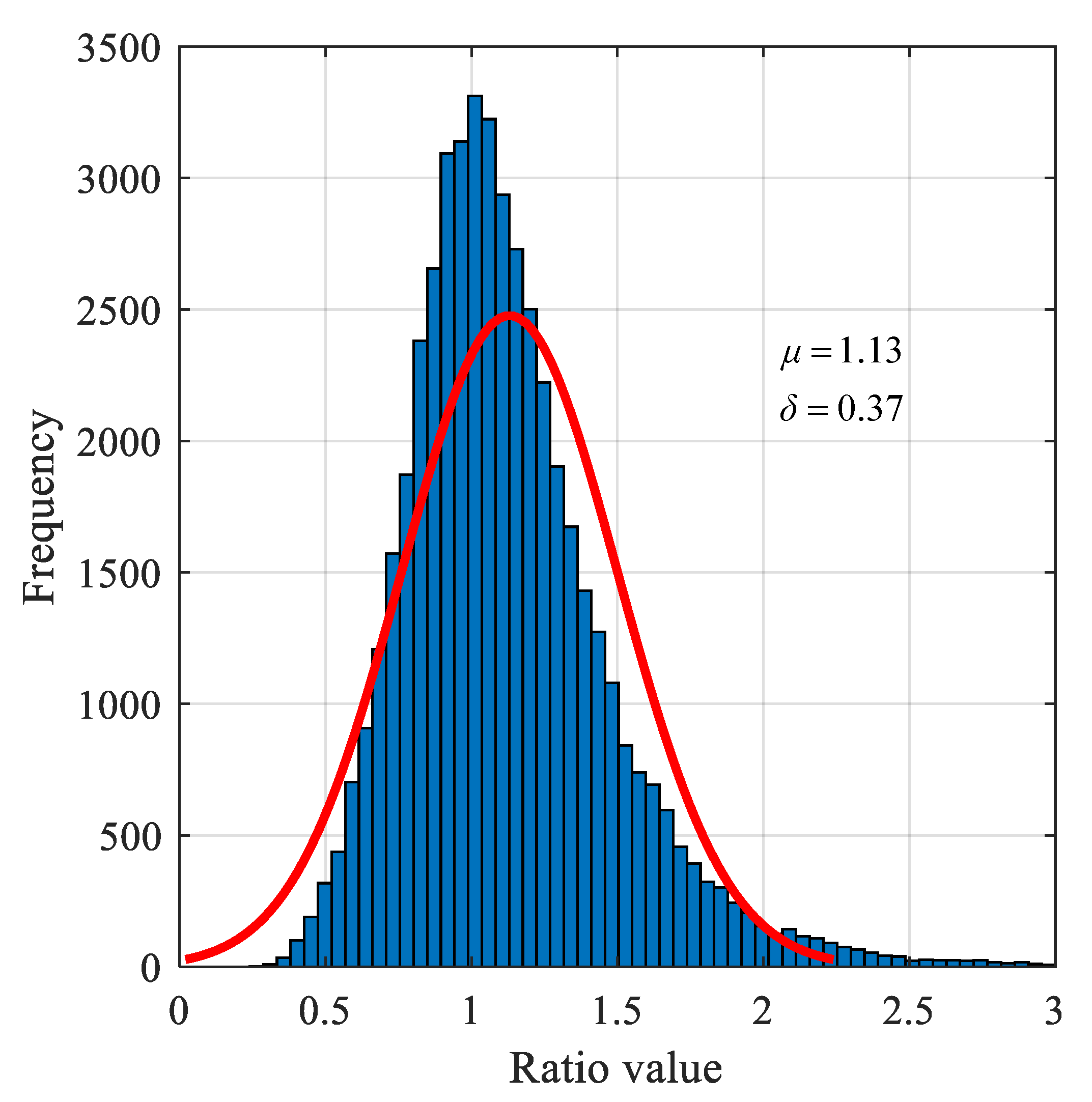
3.2. Determination of Automatic Classification Threshold for Glacial Lakes

The RII we generated in the previous section is based on the averaging of multi-temporal intensity images selected when the basins of glacial lakes are entirely exposed, which means that the coverage areas of glacial lakes and the surroundings in the RII have similar intensity values. When meltwater converged in the glacial lakes, the values of pixels corresponding to the glacial lakes in the ratio maps were exponentially amplified due to the specular reflection of the water surface, while those for the non-glacial lake areas remained unchanged. Thus, we suggest applying the upper confidence interval of the stacked ratio maps corresponding to the non-glacial lake area samples.
In this case, we used the identified non-glacial lake area in the zone “T” (16 by 21 pixels) shown in Figure 3a as the samples for threshold calculation. The histogram of the samples with 48384-pixel values and the fitted normal density function curve is shown in Figure 5. We calculated the mean and standard deviation using the maximum likelihood estimator and then computed the inverse of cumulative distribution function values evaluated at the probability values of 0.997 and its 95% confidence interval for the normal distribution. Finally, 2.14 and 2.15 were solved as the lower and upper confidence bounds, respectively, and 2.15 was used as the fixed threshold for classifying the time series of ratio maps.

3.3. Accuracy Evaluation

We present to suppose the boundaries of the glacial lakes derived from Sentinel-2A/B optical images as the ground truth to validate the accuracy of the proposed method. The normalized difference water index (NDWI) was employed as an indicator for classifying the glacial lakes. NDWI, defined by McFeeters [17], is a normalized ratio index between the green band and near-infrared (NIR) band that has been widely used in the classification of the water for glacial lakes [6,7,8,10,11,12,13], which is defined as
NDWI = ρ G r e e n ρ NIR ρ Green + ρ NIR
where ρ G r e e n and ρ NIR denote the green band and NIR band, respectively; for Sentinel-2 A/B, they are corresponding to the band 3 and band 8 [48].
With the characteristics of the strong absorption in the NIR band and the high reflectivity in the green band of water, the contrast between the water bodies and their vicinities was enhanced in the NDWI map [17,49]. However, the threshold for further classification of glacial lakes based on NDWI varies depending on the local geomorphic conditions. Furthermore, considering that some of the images were acquired without water cover in the basins of glacial lakes, we suggest classifying the time series of NDWI maps using a uniform fixed threshold.
In this case, to ensure the accuracy for classifying the glacial lakes based on the time series of NDWI maps, we tested and applied Otsu’s method for post-processing classification [50]. Otsu’s method is used to perform automatic image thresholding and returns a single intensity threshold that separates pixels into two classes determined by iteratively computing to minimize the intra-class intensity variance. We first selected the nine NDWI maps with the water storage areas by visual interpretation and automatically calculated their thresholds utilizing Otsu’s method image by image, then averaged these nine estimated values as the global threshold for classifying the time series of NDWI maps. Finally, we calculated the relative error of area between the results and the outlines of glacial lakes identified based on the proposed method as the accuracy for evaluation.

4. Experiment and Result

4.1. Classification Results and Dynamic Changes of XGL and DGL

We calculated the time series of ratio maps based on the proposed method for the 144 co-registration SAR images shown in Figure 6 and then binarized them using the threshold obtained in Section 3.2. To further eliminate the disturbance of speckle noise and small supraglacial ponds, we removed the objects with the area of connected components containing fewer than 16 pixels for the results after classification. Then, we used the DEM to complete the projection transformation of the Range–Doppler coordinate to the WGS-84 UTM zone 47N coordinate for the binarized ratio maps. Finally, we resampled the geocoded binarized ratio maps to the 10-m-grid resolution, the same as the Sentinel-2 satellite images. The projection conversion was performed after the classification was completed because the speckle noises were involved in the resampling process and exacerbated in the geocoded results.
Figure 7 shows the time series of classification results of DGL and XGL. The blue and green in each subgraph represent the areas covered by the glacial lake and the non-glacial lake, respectively. Moreover, the time series of boundaries of XGL and DGL, automatically delineated by the edge detection operator, were also mapped and shown as the white polygons superimposed in Figure 7. We computed the areas of XGL and DGL derived from each period of SAR images, respectively. Furthermore, their annual dynamic changes between 2015 and 2020 are shown in Figure 8. During this period, the observed largest area of XGL was 69,100 m2 on 24 August 2020, and that for DGL was 74,440 m2 on 14 August 2017.
We observed periodic water recharging and discharging processes within the dynamic changes of XGL and DGL between 2014 and 2020. The recharging process of XGL began from late April to early May each year. The water area increased rapidly in June and reached its maximum in August or September and then remained stable for about two months until October. Subsequently, the area of XGL gradually shrank until the water body completely disappeared in February of the following year. The pattern of dynamic change for DGL was similar to that of XGL from 2014 to 2017. The water of DGL was rapidly filled from June to July and wholly discharged in November. However, the pattern of periodic water recharge–maintain–discharge was interrupted from 2018. The stage of dynamic stability of the water area was no longer observed. In 2019 and 2020, the maximum water storage area of DGL was surveyed with only 36,600 m2 on 25 June 2020.
We counted the annual maximum water storage area, and corresponding dates for XGL and DGL observed from 2015 to 2020, as shown in Table 1. During this period, the largest annual water area of XGL showed a remarkable increasing trend with an average annual growth rate of 3.19%. Compared with 2015, the largest water area of DGL increased by 25.25% in 2017 (equivalent to 12.63% annually). However, with the anomalous variation of DGL in July 2018, the increasing trend of DGL was also interrupted.

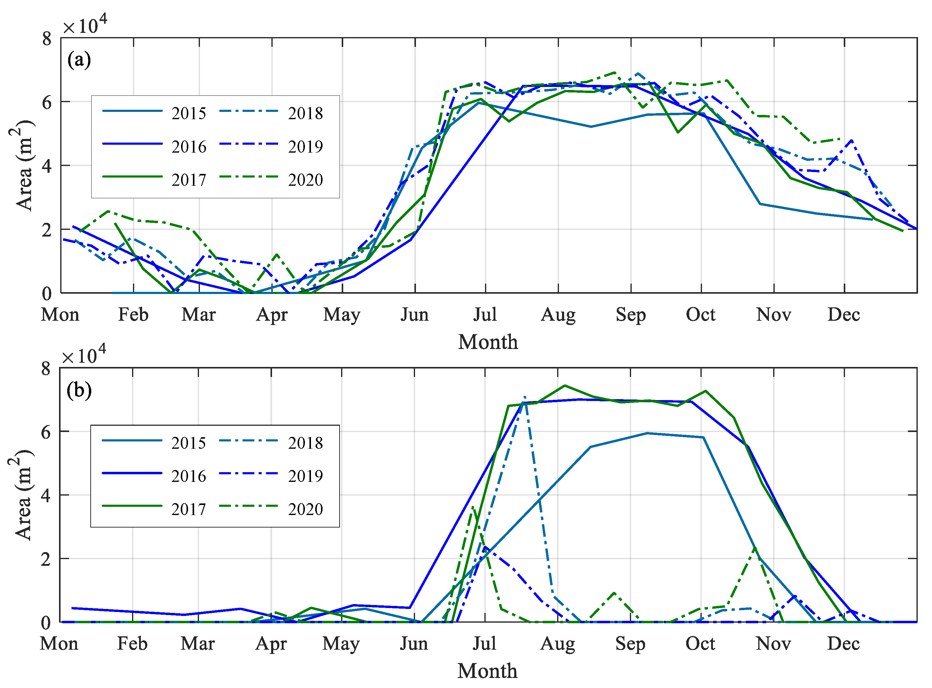
4.2. The Spatiotemporal Evolution Characteristics of DGL and XGL

To explore the phenomenon of periodic water recharge and discharge for XGL and DGL, the daily temperature and precipitation data were used for the correlation analysis with changes in the glacial lakes. Corresponding to the study area and the period of SAR image acquisition, the in situ data recorded by the Jiulong County Meteorological Station (29°00′N, 101°30′E, ~3000 m) in Sichuan Province were also acquired from October 2014 to November 2020. Considering that the altitude of Jiulong Station is about 1000 m lower than the terminus of Gongba Glacier, linear correction was conducted for the recorded temperature data by using the standard temperature lapse rate of −6.49° per 1000 m. Since the precipitation is only used as a reference for qualitative analysis, the variation in precipitation with altitude is assumed to be ignored in this study.
Figure 9a,b show the dynamic area changes of XGL and DGL from October 2014 to November 2020, respectively. The corrected monthly average temperature and monthly accumulated precipitation over the same period are both overlaid in Figure 9. We calculated the Pearson correlation coefficient between these observations to quantitatively analyze the interrelationship between the changes in the glacial lake area and the typical climatic factors, i.e., temperature and precipitation. The correlation coefficients of XGL with temperature and precipitation were 0.65 and 0.64, respectively, and these values were 0.39 and 0.42 for DGL. However, if the monitoring period was divided into two segments on January 1, 2018, the correlation coefficients of the former would be 0.64 and 0.52, respectively, while the values of the latter would be 0.25 and 0.32. These suggest that precipitation and meltwater are important nutrition for glacial lake formation and periodic water recharge. Furthermore, considering that precipitation had a decreasing trend in recent years, the spreading of XGL and DGL also reflects an acceleration of glacial meltwater, representing an aggravation of Gongba Glacier ablation.
The melting of snow and ice on the Gongba Glacier began in March every year with the temperature rising above 0 °C. Since May, the temperature continued warming and was accompanied by enhanced precipitation. The glacier entered a strong ablation phase, part of the meltwater flowed into the downstream river through the subglacial drainage system and some flowed into XGL and DGL through runoff from the debris-covered glacier surface. Subsequently, as the temperature further increased, the snow and ice at the higher altitudes were also beginning to melt, and the rainfall intensity also increased significantly. Thus, the replenishment of abundant meltwater induced the area of XGL and DGL to expand rapidly.
To inquire about the cause of the periodic water discharge of glacial lakes, we made two field trips to the Gongba Glacier on June 9 and October 17, 2018. Numerous exposed ice cliffs and entrances of the subglacial drainage system were identified at the bottom of the DGL basin (see Figure 10), which confirmed that the glacial lake basin was composed of buried dead ice and thick moraines. After the meltwater gathered in the glacial lake basin, the drainage tunnels were gradually dredged under water pressure and water erosion. During July and August, the recharge and discharge of glacial lakes were in a dynamic balance. However, the temperature began to drop, accompanied by the decrease in precipitation. The reduction of meltwater and rainwater resulted in the rapid shrinkage of glacial lakes. Since October, the daily average temperature gradually dropped below 0 degrees, the melting of glaciers gradually weakened, and liquid precipitation almost stagnated. XGL and DGL entered the discharge period until they disappeared completely.

4.3. Differentiation Analysis of XGL and DGL Activity Patterns

As mentioned above, the initiation of water storage of the XGL was earlier than the DGL, while its discharge was completed later than the DGL. The XGL was formed at the terminal moraine ridge of Xiaogongba Glacier, while the DGL was sited at the lateral moraine ridge of Dagongba Glacier (see Figure 1). Furthermore, we found apparent scouring traces of runoff converging to XGL on the surface of Xiaogongba Glacier during our in situ fieldwork and inferred that the XGL absorbed almost all of the meltwater and rainwater that flowed over the glacier surface based on its formation location and topography. The DGL was formed at a branch on the north side of the Dagongba Glacier and absorbed only part of the runoff, with most of the meltwater and rainwater flowing through the main body of the glacier to the terminus.
We speculate that these differences between XGL and DGL led to differences in their water storage and drainage patterns. In the early warm season each year, glacial meltwater was the primary component of the recharged water to the glacial lakes. During this period, most of the meltwater flowing over the surface of Xiaogongba Glacier converged into the XGL, while that for the Dagongba Glacier was drained directly downstream, resulting in an earlier start of water storage of the XGL than the DGL. Considering that the Dagongba Glacier is three times larger than the Xiaogongba Glacier, with increased melting of the glaciers and intensive precipitation, more water was recharged to the DGL, facilitating the rapid expansion of its area. The water replenishment in the drainage phase of the glacial lakes was similar to the storage phase, where the weakened melting of the glacier and the decreased precipitation more significantly affected the DGL.

4.4. The Glacial Lake Outburst Floods of DGL in 2018

From 24 June to 18 July 2018, DGL was quickly almost filled within 24 days and then quickly drained in the next 12 days before July 30 (see Figure 8 and Figure 9). This was significantly different from the pattern observed from 2015 to 2017. Furthermore, in the following warm seasons of 2019 and 2020, the apparent cyclical activity had not recovered. We compared the average temperature and precipitation on a month-by-month basis from 2015 to 2020 cross-sectionally, as shown in Figure 11. During this period, there were no temperature anomalies observed. In terms of precipitation, although it varied when the peak precipitation was recorded in the past six years, there were no anomalies during June and July in 2018 compared to other years.
Compared to June 2018, we found a huge new drainage entrance with an area of about 190 m2 at the bottom of the DGL basin with the benefit of drone imagery during our fieldwork in October 2018 (see Figure 12d,e). Additionally, we found an inverted triangular washed-out gap that was 47 m wide, 20 m deep, 75 m long, and 16000 m3 in volume on the lateral moraine ridge of the outer west side of the DGL (see Figure 12b,c). Considering that the downstream river channel exhibited evident traces of being washed and widened by flood, we speculate that a glacial lake outburst flood occurred in the DGL between the 18th and 30th of July 2018.
We inferred the water flow path at the time of outburst of DGL based on the orthophoto acquired by the drone on 17 October 2018, as shown in the blue lines in Figure 12a. Under years of water erosion and water pressure, the dead ice at the bottom of the DGL basin was unblocked to form a huge subglacial entrance, along with an outlet about 70 m under an ice cliff about 300 m to the west (see Figure 12f). The rushing flood washed away the lateral moraine ridge composed of loose debris deposits. Following that, the debris-laden floodwater advancing downstream along the valley resulted in a visible widening of the approximately three km-long river channels, while the debris and rocks deposited in the channel significantly altered the path of the original river flow. Additionally, a small hydroelectric installation supplying power to the Gongga Monastery and a simple bridge were destroyed in the disaster.
The XGL and DGL served as essential regulators in the water cycle of the Gongba Glacier catchment to buffer the rapid downstream dumping of meltwater. This glacial lake outburst event severely changed the activity cycle of DGL. Both in 2019 and 2020, the DGL burst again before it was filled. The area expansion of XGL and DGL responded to the accelerated melting of the Gongba Glacier in the context of climate warming and reflected the potential disasters of the expanding glacial lakes in the southeast Tibetan Plateau.

4.5. Comparison of Classification Results with Optical Images and Accuracy Assessment

For the data used in this study, since the Sentinel-1 and Sentinel-2 satellites had different revisit intervals, only three times were available where these two satellites collected data on the same day, 23 August 2018, 22 October 2018, and 11 October 2020. We generated their color images, NDWI maps, classification results based on NDWI, SAR images, ratio maps, and classification results based on the proposed method and overlaid boundaries derived from the different methods for visual comparison, shown in Figure 13. The overlaid boundaries shown in the last column of Figure 13 indicate the consistency of the results derived from these two different methods. For an example of the images acquired from 22 October 2018 (second row of Figure 13), an isolated island was exposed in the XGL during the discharged phase and observed on both optical and SAR images with similar outlines. The area changes of XGL and DGL are superimposed in Figure 9a,b, respectively. Comparison between the areas of the glacial lake extracted by Sentinel-1 and Sentinel-2 showed remarkable similarity, and the time series of these two classified results also showed a consistent trend.
However, there were some differences between the boundaries mapped based on SAR images and optical images. (1) The shape of glacial lakes is slightly inconsistent because of the unique geometric distortion and projection distortion of the side-looking imaging SAR system. (2) The glacial lakes area varies because of the different spatial resolutions and separate data processes of these two satellites. Table 2 shows the areas and the differences of the XGL extracted from the three-period optical and SAR images. We assume the results derived from NDWI maps to be the ground truth and calculate the relative error of area for the outlines identified based on the proposed method. The testing results show that the accuracy for identifying the outlines of the glacial lakes with Sentinel-1A SAR images can reach up to 96.49%.

5. Discussion

In this contribution, we developed and showed the use of a simple but effective data processing method for classifying glacial lakes and monitoring their dynamic evolution using time series of SAR images acquired by the Sentinel-1 A satellite for two glacial lakes at the terminus of Gongba Glacier. Instead of calculating thresholds directly using SAR intensity images, we improved the neighborhood ratio model to enhance the contrast between water bodies and their surroundings in each SAR image. Based on the proposed method, we recovered the entire process of area change of these two glacial lakes from 2014 to 2020 and analyzed their evolutionary characteristics by comparing UAV images and meteorological data.
Approximately 6 years of Sentinel-1 A SAR images were used for monitoring the dynamic evolution of the glacial lakes and further addressing the spatio-temporal behavior, e.g., filling, expansion, and even outburst. A series of results showed that the proposed method has excellent persistence and adaptability in this typical application. Above all, the periodic filling and release processes can be tracked for these two lakes, as well as their expansion and the outburst. Furthermore, the proposed method can be developed into an automated processing procedure that allows the acquired data to be used in a real-time environment, which further makes timely and reliable GLOF risk evaluation under the high-frequency SAR image acquisition condition.
The intensity values of homogeneous regions in SAR images could be assumed to follow an approximately log-normal distribution [51]. When the water and non-water bodies in the SAR scene are comparable, the optimal threshold can be calculated utilizing the nature of the bimodal distribution of the log-transformed intensity images. Most of the current methods aim to ensure that the number of samples involved in the optimal threshold calculation is comparable between the water body and the surroundings, as previous authors have investigated [52,53]. However, images with histograms having extremely unequal peaks or only one peak are unsuitable for this assumption, as in this study when the water of the two glacial lakes was about to release or completely released. The proposed method does not respect the distribution of image intensity values and can effectively reduce such errors. Furthermore, the design of RII in the NR model enables the involved SAR images to be under the same criteria, which ensures it is possible to classify multi-temporal SAR images using a single fixed threshold. The developed method allows the classification of glacial lakes in the area of interest, regardless of the specific gravity of the water area in the SAR scene, even for zero.
Regardless of the different imaging modes used, the removal topography-induced effects should be an important factor in the automatic classification of the glacial lake. Basically, features located on the slope facing the radar present higher intensity compared to the intensity from that located in areas of shadow. These noises are often corrected by calculating the local incidence angle and the pixel area normalization factor based on the DEM, as described by O’Grady et al. [54]. Instead of direct correction of backscattered intensity, this study reduces these noises using the same imaging geometry between the generated RII and each SAR image for ratio offset. The proposed method simplifies the data processing and is efficient, avoiding the error propagation caused by the resolution and accuracy of the DEM.
One of the objectives of the proposed method was to develop a generic processing chain applicable to the dynamic monitoring of various types of glacial lakes. In the current work, we studied a pair of types with periodic filling and release, both of them with distinct periods of complete release, providing a basis for the RII generation. For periodic freeze–thaw glacial lakes, the frozen glacial lake surface would become rough and present a backscattering intensity similar to that of the surroundings when snow is attached to it. The work in this paper can be directly applied to such cases since the images acquired after the freezing of the glacial lake can be assumed as zero-area. However, the proposed method may not be available for the glacial lake where liquid water exists all year round, which would present a challenge in knowing how to select the images to generate the RII. Therefore, it may be necessary to adapt the current method so that the zero-area represented by the RII is no longer an underlying condition. For example, multiple images with the smallest area of the glacial lake are visually interpreted to generate the RII, and then the optimal threshold or manual digitization is used to produce a mask representing the RII water area. The area of change is accumulated on the basis of the mask area during the classification of the glacial lake. In addition, this approach can be further extended to rapid assessment of flooded areas using the RII produced from SAR images before the rainy season.
Nevertheless, given the small size of the two glacial lakes studied, we did not consider the wind-induced effect on the backscattered intensity from the water surface. Indeed, wind may influence the smoothness of the water surface, causing a change in the local incidence angle of the radar and, thus, a change in the backscattered intensity [55]. In addition, we also did not consider whether the turbidity of the glacial lake water bodies would influence the classification results for lack of ground truth data. Therefore, the robustness of the new method needs to be tested on more different types of glacial lakes. This task will be studied in future work.

6. Conclusions

In this study, we proposed an improved neighborhood-based ratio method to map the boundaries of glacial lakes and detect their spatiotemporal evolution based on the time series of SAR images. We first generated the reference intensity image by averaging the SAR images that selected the water of glacial lakes when it was discharged entirely, and then calculated the ratio between the reference intensity image and the time series of SAR images after smoothing filtering image by image. Two glacial lakes at the terminus of the Gongba Glacier in the southeastern Tibetan Plateau were selected as the study site, and we achieved the mapping and dynamic monitoring of the two glacial lakes based on 144 Sentinel-1A SAR images acquired from 2014 to 2020.
Through neighborhood ratio operations, the proposed method has advantages in reducing the influences of the topography-induced effects and speckle noises, as well as amplifying inter-class differences between glacial lakes and surroundings. The shared reference intensity image ensures the possibility of classifying water bodies with a single fixed threshold for time series of ratio maps, thus, ensuring the validity and accuracy of glacial lake classification regardless of the percentage of water area in the SAR scene. Furthermore, by comparing the results derived from the multispectral images acquired from Sentinel-2 A/B satellites, the accuracy for identifying the boundaries of the glacial lakes with Sentinel-1A SAR images averaged 96.49%.
Our study covered the entire ascending orbit data of Sentinel-1 A satellite during the monitoring period, recovering the dynamic evolution of the glacial lakes in the study area, including one GLOF. Relevant results showed that the developed data processing chain has excellent persistence and adaptability in addressing glacial lake dynamics monitoring. Furthermore, timely and reliable GLOF risk evaluation can be conducted under the high-frequency SAR image acquisition condition.

Author Contributions

Conceptualization, B.Z., G.L., and R.Z.; methodology, B.Z.; validation, B.Z. and Y.F.; investigation, B.Z., Q.L., and J.C.; data curation, B.Z. and Y.F.; writing—original draft preparation, B.Z.; writing—review and editing, B.Z., G.L., R.Z., X.W., and Z.L.; funding acquisition, G.L., Q.L., and X.W. All authors have read and agreed to the published version of the manuscript.

Funding

This research was jointly funded by the National Natural Science Foundation of China (Grant Number: 41771402, 41871069, 42071410, 41804009) and National Key R&D Program of China, (Grant Number: 2017YFB0502700).

Institutional Review Board Statement

Not applicable.

Informed Consent Statement

Not applicable.

Data Availability Statement

Data is contained within the article.

Acknowledgments

The Sentinel-1 and Sentinel-2 A/B satellite images were provided by the Copernicus mission of the European Space Agency. The SRTM DEM data was downloaded from the United States Geological Survey. The temperature and precipitation data recorded by the Jiulong County Meteorological Station were provided by the China Meteorological Data Service Center (http://data.cma.cn/). The outlines of the Gongba Glacier were provided by National Cryosphere Desert Data Center. (http://www.ncdc.ac.cn).

Conflicts of Interest

The authors declare no conflict of interest.

References

  1. Shean, D.E.; Bhushan, S.; Montesano, P.; Rounce, D.R.; Arendt, A.; Osmanoglu, B. A systematic, regional assessment of high mountain Asia glacier mass balance. Front. Earth Sci. 2020, 7, 363. [Google Scholar] [CrossRef] [Green Version]
  2. Sakai, A.; Fujita, K. Contrasting glacier responses to recent climate change in high-mountain Asia. Sci. Rep. 2017, 7, 1–8. [Google Scholar] [CrossRef]
  3. Dehecq, A.; Gourmelen, N.; Gardner, A.S.; Brun, F.; Goldberg, D.; Nienow, P.W.; Berthier, E.; Vincent, C.; Wagnon, P.; Trouvé, E. Twenty-first century glacier slowdown driven by mass loss in High Mountain Asia. Nat. Geosci. 2019, 12, 22–27. [Google Scholar] [CrossRef]
  4. Brun, F.; Berthier, E.; Wagnon, P.; Kääb, A.; Treichler, D. A spatially resolved estimate of High Mountain Asia glacier mass balances from 2000 to 2016. Nat. Geosci. 2017, 10, 668–673. [Google Scholar] [CrossRef]
  5. Treichler, D.; Kääb, A.; Salzmann, N.; Xu, C.-Y. Recent glacier and lake changes in High Mountain Asia and their relation to precipitation changes. Cryosphere 2019, 13, 2977–3005. [Google Scholar] [CrossRef] [Green Version]
  6. Wang, X.; Siegert, F.; Zhou, A.-G.; Franke, J. Glacier and glacial lake changes and their relationship in the context of climate change, Central Tibetan Plateau 1972–2010. Glob. Planet. Chang. 2013, 111, 246–257. [Google Scholar] [CrossRef]
  7. Wang, W.; Gao, Y.; Anacona, P.I.; Lei, Y.; Xiang, Y.; Zhang, G.; Li, S.; Lu, A. Integrated hazard assessment of Cirenmaco glacial lake in Zhangzangbo valley, Central Himalayas. Geomorphology 2018, 306, 292–305. [Google Scholar] [CrossRef]
  8. Veh, G.; Korup, O.; Von Specht, S.; Roessner, S.; Walz, A. Unchanged frequency of moraine-dammed glacial lake outburst floods in the Himalaya. Nat. Clim. Chang. 2019, 9, 379–383. [Google Scholar] [CrossRef]
  9. Nie, Y.; Liu, Q.; Wang, J.; Zhang, Y.; Sheng, Y.; Liu, S. An inventory of historical glacial lake outburst floods in the Himalayas based on remote sensing observations and geomorphological analysis. Geomorphology 2018, 308, 91–106. [Google Scholar] [CrossRef]
  10. Nie, Y.; Sheng, Y.; Liu, Q.; Liu, L.; Liu, S.; Zhang, Y.; Song, C. A regional-scale assessment of Himalayan glacial lake changes using satellite observations from 1990 to 2015. Remote. Sens. Environ. 2017, 189, 1–13. [Google Scholar] [CrossRef] [Green Version]
  11. Li, J.; Sheng, Y. An automated scheme for glacial lake dynamics mapping using Landsat imagery and digital elevation models: A case study in the Himalayas. Int. J. Remote. Sens. 2012, 33, 5194–5213. [Google Scholar] [CrossRef]
  12. Liu, Q.; Guo, W.; Nie, Y.; Liu, S.; Xu, J. Recent glacier and glacial lake changes and their interactions in the Bugyai Kangri, southeast Tibet. Ann. Glaciol. 2016, 57, 61–69. [Google Scholar] [CrossRef] [Green Version]
  13. Moussavi, M.; Pope, A.; Halberstadt, A.; Trusel, L.; Cioffi, L.; Abdalati, W. Antarctic Supraglacial Lake Detection Using Landsat 8 and Sentinel-2 Imagery: Towards Continental Generation of Lake Volumes. Remote. Sens. 2020, 12, 134. [Google Scholar] [CrossRef] [Green Version]
  14. Doxaran, D.; Froidefond, J.-M.; Lavender, S.; Castaing, P. Spectral signature of highly turbid waters. Remote. Sens. Environ. 2002, 81, 149–161. [Google Scholar] [CrossRef]
  15. Feyisa, G.L.; Meilby, H.; Fensholt, R.; Proud, S.R. Automated Water Extraction Index: A new technique for surface water mapping using Landsat imagery. Remote. Sens. Environ. 2014, 140, 23–35. [Google Scholar] [CrossRef]
  16. Frohn, R.C.; Hinkel, K.M.; Eisner, W.R. Satellite remote sensing classification of thaw lakes and drained thaw lake basins on the North Slope of Alaska. Remote. Sens. Environ. 2005, 97, 116–126. [Google Scholar] [CrossRef]
  17. McFeeters, S.K. The use of the Normalized Difference Water Index (NDWI) in the delineation of open water features. Int. J. Remote. Sens. 1996, 17, 1425–1432. [Google Scholar] [CrossRef]
  18. Huggel, C.; Kääb, A.; Haeberli, W.; Teysseire, P.; Paul, F. Remote sensing based assessment of hazards from glacier lake outbursts: A case study in the Swiss Alps. Can. Geotech. J. 2002, 39, 316–330. [Google Scholar] [CrossRef] [Green Version]
  19. Rogers, A.S.; Kearney, M.S. Reducing signature variability in unmixing coastal marsh Thematic Mapper scenes using spectral indices. Int. J. Remote. Sens. 2004, 25, 2317–2335. [Google Scholar] [CrossRef]
  20. Xu, H. Modification of normalised difference water index (NDWI) to enhance open water features in remotely sensed imagery. Int. J. Remote. Sens. 2006, 27, 3025–3033. [Google Scholar] [CrossRef]
  21. Bhardwaj, A.; Singh, M.K.; Joshi, P.; Snehmani; Singh, S.; Sam, L.; Gupta, R.; Kumar, R. A lake detection algorithm (LDA) using Landsat 8 data: A comparative approach in glacial environment. Int. J. Appl. Earth Obs. Geoinf. 2015, 38, 150–163. [Google Scholar] [CrossRef]
  22. Uhlmann, S.; Kiranyaz, S. Integrating Color Features in Polarimetric SAR Image Classification. IEEE Trans. Geosci. Remote. Sens. 2013, 52, 2197–2216. [Google Scholar] [CrossRef]
  23. Adeli, S.; Salehi, B.; Mahdianpari, M.; Quackenbush, L.; Brisco, B.; Tamiminia, H.; Shaw, S. Wetland Monitoring Using SAR Data: A Meta-Analysis and Comprehensive Review. Remote. Sens. 2020, 12, 2190. [Google Scholar] [CrossRef]
  24. Gong, M.; Li, Y.; Jiao, L.; Jia, M.; Su, L. SAR change detection based on intensity and texture changes. ISPRS J. Photogramm. Remote. Sens. 2014, 93, 123–135. [Google Scholar] [CrossRef]
  25. Strozzi, T.; Wiesmann, A.; Kaab, A.; Joshi, S.; Mool, P.K. Glacial lake mapping with very high resolution satellite SAR data. Nat. Hazards Earth Syst. Sci. 2012, 12, 2487–2498. [Google Scholar] [CrossRef] [Green Version]
  26. Ferretti, A.; Monti-guarnieri, A.; Prati, C.; Rocca, F. InSAR Principles: Guidelines for SAR Interferometry Processing and Interpretation, Part C. InSAR Processing: A Mathematical Approach; ESA Publications: Auckland, New Zealand, 2007. [Google Scholar]
  27. Miles, K.E.; Willis, I.C.; Benedek, C.L.; Williamson, A.G.; Tedesco, M. Toward Monitoring Surface and Subsurface Lakes on the Greenland Ice Sheet Using Sentinel-1 SAR and Landsat-8 OLI Imagery. Front. Earth Sci. 2017, 5, 58. [Google Scholar] [CrossRef] [Green Version]
  28. Zhang, M.; Chen, F.; Tian, B.; Liang, D.; Yang, A. High-Frequency Glacial Lake Mapping Using Time Series of Sentinel-1A/1B SAR Imagery: An Assessment for the Southeastern Tibetan Plateau. Int. J. Environ. Res. Public Health 2020, 17, 1072. [Google Scholar] [CrossRef] [Green Version]
  29. Zhang, M.; Chen, F.; Tian, B.; Liang, D.; Yang, A. Characterization of Kyagar Glacier and Lake Outburst Floods in 2018 Based on Time-Series Sentinel-1A Data. Water 2020, 12, 184. [Google Scholar] [CrossRef] [Green Version]
  30. Zhang, Y.; Zhang, G.; Zhu, T. Seasonal cycles of lakes on the Tibetan Plateau detected by Sentinel-1 SAR data. Sci. Total Environ. 2020, 703, 135563. [Google Scholar] [CrossRef]
  31. Teillet, P.; Guindon, B.; Meunier, J.-F.; Goodenough, D. Slope-aspect effects in synthetic aperture radar imagery. Can. J. Remote. Sens. 1985, 11, 39–49. [Google Scholar] [CrossRef]
  32. Ulander, L. Radiometric slope correction of synthetic-aperture radar images. IEEE Trans. Geosci. Remote. Sens. 1996, 34, 1115–1122. [Google Scholar] [CrossRef]
  33. Castel, T.; Beaudoin, A.; Stach, N.; Stussi, N.; Le Toan, T.; Durand, P. Sensitivity of space-borne SAR data to forest parameters over sloping terrain. Theory and experiment. Int. J. Remote. Sens. 2001, 22, 2351–2376. [Google Scholar] [CrossRef]
  34. Gong, M.; Cao, Y.; Wu, Q. A Neighborhood-Based Ratio Approach for Change Detection in SAR Images. IEEE Geosci. Remote. Sens. Lett. 2012, 9, 307–311. [Google Scholar] [CrossRef]
  35. Ma, J.; Gong, M.; Zhou, Z. Wavelet Fusion on Ratio Images for Change Detection in SAR Images. IEEE Geosci. Remote. Sens. Lett. 2012, 9, 1122–1126. [Google Scholar] [CrossRef]
  36. Bazi, Y.; Bruzzone, L.; Melgani, F. Automatic Identification of the Number and Values of Decision Thresholds in the Log-Ratio Image for Change Detection in SAR Images. IEEE Geosci. Remote. Sens. Lett. 2006, 3, 349–353. [Google Scholar] [CrossRef] [Green Version]
  37. Xie, H.; Pierce, L.; Ulaby, F. SAR speckle reduction using wavelet denoising and Markov random field modeling. IEEE Trans. Geosci. Remote. Sens. 2002, 40, 2196–2212. [Google Scholar] [CrossRef] [Green Version]
  38. Pan, B.T.; Zhang, G.L.; Wang, J.; Cao, B.; Geng, H.P.; Zhang, C.; Ji, Y.P. Glacier changes from 1966–2009 in the Gongga Mountains, on the south-eastern margin of the Qinghai-Tibetan Plateau and their climatic forcing. Cryosphere 2012, 6, 1087–1101. [Google Scholar] [CrossRef] [Green Version]
  39. Su, Z.; Liang, D.; Hong, M. Developing conditions, amounts and distributions of glaciers in Gongga Mountains. J. Glaciol. Glaciol. 1993, 15, 551–558. (In Chinese) [Google Scholar]
  40. Zhang, N.; He, Y.; Duan, K.; Pang, H.; Li, Z. Changes of Gongba Glacier in the west slope of Mt. Gongga during the past 25 years. J. Glaciol. Glaciol. 2008, 30, 380–382. (In Chinese) [Google Scholar]
  41. Liu, S.; Guo, W.; Xu, J. The Second Glacial Catalogue Data set of China (v1.0). National Cryosphere Desert Data Center, 2019. Available online: www.ncdc.ac.cn (accessed on 15 February 2021).
  42. Kang, J. The Characteristics and Forming Process of Glacial Peripheral Moraines at Gongba Glaciers in Mt. Gonngga. J. Glaciol. Glaciol. 1989, 2, 172–176. (In Chinese) [Google Scholar]
  43. Cao, Z. The Hydrologic Characteristics of the Gongba Glacier in the Mount Gongga Area. J. Glaciol. Glaciol. 1988, 10, 57–65. (In Chinese) [Google Scholar]
  44. Torres, R.; Snoeij, P.; Geudtner, D.; Bibby, D.; Davidson, M.; Attema, E.; Potin, P.; Rommen, B.; Floury, N.; Brown, M.; et al. GMES Sentinel-1 mission. Remote Sens. Environ. 2012, 120, 9–24. [Google Scholar] [CrossRef]
  45. Drusch, M.; Del Bello, U.; Carlier, S.; Colin, O.; Fernandez, V.; Gascon, F.; Hoersch, B.; Isola, C.; Laberinti, P.; Martimort, P.; et al. Sentinel-2: ESA’s Optical High-Resolution Mission for GMES Operational Services. Remote. Sens. Environ. 2012, 120, 25–36. [Google Scholar] [CrossRef]
  46. Yao, X.; Liu, S.; Han, L.; Sun, M.; Zhao, L. Definition and classification system of glacial lake for inventory and hazards study. J. Geogr. Sci. 2018, 28, 193–205. [Google Scholar] [CrossRef] [Green Version]
  47. Wegnüller, U.; Werner, C.; Strozzi, T.; Wiesmann, A.; Frey, O.; Santoro, M. Sentinel-1 Support in the GAMMA Software. Procedia Comput. Sci. 2016, 100, 1305–1312. [Google Scholar] [CrossRef] [Green Version]
  48. Yang, X.; Zhao, S.; Qin, X.; Zhao, N.; Liang, L. Mapping of Urban Surface Water Bodies from Sentinel-2 MSI Imagery at 10 m Resolution via NDWI-Based Image Sharpening. Remote. Sens. 2017, 9, 596. [Google Scholar] [CrossRef] [Green Version]
  49. McFeeters, S.K. Using the Normalized Difference Water Index (NDWI) within a Geographic Information System to Detect Swimming Pools for Mosquito Abatement: A Practical Approach. Remote. Sens. 2013, 5, 3544–3561. [Google Scholar] [CrossRef] [Green Version]
  50. Otsu, N. A threshold selection method from gray-level histograms. IEEE Trans. Syst. Man, Cybern. 1979, 9, 62–66. [Google Scholar] [CrossRef] [Green Version]
  51. Ball, G.H.; Hall, D.J. A clustering technique for summarizing multivariate data. Syst. Res. Behav. Sci. 1967, 12, 153–155. [Google Scholar] [CrossRef]
  52. Vickers, H.; Malnes, E.; Høgda, K.-A. Long-Term Water Surface Area Monitoring and Derived Water Level Using Synthetic Aperture Radar (SAR) at Altevatn, a Medium-Sized Arctic Lake. Remote. Sens. 2019, 11, 2780. [Google Scholar] [CrossRef] [Green Version]
  53. Liang, J.; Liu, D. A local thresholding approach to flood water delineation using Sentinel-1 SAR imagery. ISPRS J. Photogramm. Remote. Sens. 2020, 159, 53–62. [Google Scholar] [CrossRef]
  54. O’Grady, D.; Leblanc, M.; Gillieson, D. Relationship of local incidence angle with satellite radar backscatter for different surface conditions. Int. J. Appl. Earth Obs. Geoinf. 2013, 24, 42–53. [Google Scholar] [CrossRef]
  55. O’Grady, D.; Leblanc, M.; Bass, A. The use of radar satellite data from multiple incidence angles improves surface water mapping. Remote. Sens. Environ. 2014, 140, 652–664. [Google Scholar] [CrossRef]
Figure 1. (a) The topography and location of the study area, the blue dotted polygons show outlines of the Gongba Glacier. (b) The Google Earth image of the Xioagongba Glacial Lake (XGL) and Dagongba Glacial Lake (DGL) acquired on 5 October 2017, corresponding to the red rectangular box in (a).
Remotesensing 13 01313 g001
Figure 2. The flow chart of data processing for identifying the boundaries of glacial lakes based on proposed method. SAR N f and ratio N f denote the smoothed filtered synthetic aperture radar (SAR) image and the binarized classified ratio map, respectively.
Remotesensing 13 01313 g002
Figure 3. (a) The generated reference intensity image, the blue dotted lines indicate the shapes of XGL and DGL. (b) The intensity map in the 8-bit format acquired on 9 August 2016, the yellow lines indicate the position of profiles corresponding to Figure 4. (c) The intensity color relief map corresponding to (b). (d) The ratio color relief map for 9 August 2016.
Remotesensing 13 01313 g003
Figure 4. (a,c) show the distributions of intensity values along the yellow profile lines “H” and “V” in Figure 3b based on the intensity map, respectively. (b,d) show the profiles of the same lines corresponding to (a,c) in the ratio map, respectively. The green, blue, and red dotted lines represent non-glacial lakes, glacial lakes, and misclassification under the condition of using a threshold by manual.
Remotesensing 13 01313 g004
Figure 5. The histogram (blue bars) and the fitted normal density function curve (red line) of samples selected in the zone “T” (16 by 21 pixels) are shown in Figure 3. Note: μ and δ represent the mean and standard deviation, respectively.
Remotesensing 13 01313 g005
Figure 6. The 144 ratio maps derived from the 144 Sentinel-1 A SAR images based on the proposed method. The upper left corner of each sub-figure shows the date when the corresponding SAR image was acquired, in the format of “yyyymmdd”. The color bar indicates the ratio level ranging from 0 to 5, noting that the values greater than 5 are also colored with the same exponent as 5. The region with a high ratio level represents the water surface.
Remotesensing 13 01313 g006
Figure 7. The results after the classification of glacial lakes corresponding to the 144 ratio maps shown in Figure 6, noting that the extracted boundaries are superimposed in each subgraph as the white outlines. The region colored in green represents the non-glacial lake area, while blue represents the glacial lake area. The upper left corner of each sub-figure shows the date when the corresponding SAR image was acquired, in the format of “yyyymmdd”. The lower right corner of each sub-figure is marked with its dynamic status in the cycle. and indicate that it is filling and discharging, and ○ indicating it is dynamically stable and completely drained.
Remotesensing 13 01313 g007
Figure 8. (a,b) show the annual water area changes of the XGL and DGL between 2015 and 2020, respectively. The curves corresponding to each year are superimposed for visual comparison.
Remotesensing 13 01313 g008
Figure 9. (a,b) show the XGL and DGL area changes from October 2014 to November 2020, respectively. The blue and green dotted lines represent the corrected monthly average temperature and monthly cumulative precipitation changes, recorded by Jiulong Station. The pink lines and the scattered triangles represent the spatiotemporal changes of glacial lakes calculated based on the Sentinel-1 SAR images and the Sentinel-2A/B optical images.
Remotesensing 13 01313 g009
Figure 10. Photos of the DGL on the field survey on 17 October 2018. (a,b) show the two entrances of the drainage tunnel at the basin of the DGL. The yellow dotted lines show the estimated entrance radius.
Remotesensing 13 01313 g010
Figure 11. (a,b) show the comparison of monthly mean temperature and cumulative precipitation from 2015 to 2020, respectively.
Remotesensing 13 01313 g011
Figure 12. (a) The drainage path of the glacial lake outburst flood in July 2018 for the DGL, with the dashed blue lines being the conjectured subglacial channel, the solid blue lines being drawn based on flood scour traces, and the cyan dotted line showing the outline of the DGL. (b,c) are orthophotos based on images acquired by drones on June 9 and October 17, 2018, respectively, with the red dotted line showing the flood-damaged surface area. (d,e) are orthophotos of the new, large drainage entrance at the bottom of the DGL basin on 9 June and 17 October 2018, respectively, with the yellow line showing the outline of this drainage entrance. (f) shows the outlet of the DGL outburst flood.
Remotesensing 13 01313 g012
Figure 13. Comparison of glacial lake classification results between SAR images and optical images acquired on the same day. The first to third columns are the true color images, the NDWI color relief maps, and the classification results derived from NDWI maps. The fourth to sixth columns are the 8-bit SAR intensity maps, the ratio color relief maps, and the classified binary maps based on SAR images. The seventh column is the comparison of the glacial lake boundaries delineated by SAR image and optical image.
Remotesensing 13 01313 g013
Table 1. Annual largest storage area and corresponding date statistics for DGL and XGL from 2015 to 2020. The variation is calculated by subtracting the area of the two adjacent years.
XGLDGL
YearMax AreaVariationDateMax AreaVariationDate
201559,600 m2/2015-06-2859,400 m2/2015-09-08
201664,900 m2+5300 m22016-07-1670,000 m2+10,6002016-08-09
201765,500 m2+600 m22017-09-0974,400 m2+44002017-08-04
201868,800 m2+3300 m22018-09-0471,000 m2−34002018-07-18
201966,000 m2−2800 m22019-07-0123,700 m2−47,3002019-07-01
202069,100 m2+3100 m22020-08-2436,600 m2+12,9002020-06-25
Table 2. Comparison of the area of the XGL extracted from Sentinel-2 A/B optical images with that extracted from Sentinel-1 SAR image acquired on the same day.
DateSentinel-2 A/BSentinel-1DifferenceAccuracy
23 August 2018,64,500 m262,400 m2−2100 m296.74%
22 October 201849,900 m246,800 m2−3100 m293.79%
11 October 202065,900 m266,600 m2700 m298.94%
//Average1500 m296.49%
Publisher’s Note: MDPI stays neutral with regard to jurisdictional claims in published maps and institutional affiliations.

