
Photogrammetry Using UAV-Mounted GNSS RTK: Georeferencing Strategies without GCPs


Department of Special Geodesy, Faculty of Civil Engineering, Czech Technical University in Prague, Thákurova 7, 166 29 Prague, Czech Republic
*
Author to whom correspondence should be addressed.
Remote Sens. 2021, 13(7), 1336; https://0-doi-org.brum.beds.ac.uk/10.3390/rs13071336
Submission received: 10 March 2021
/
Revised: 27 March 2021
/
Accepted: 28 March 2021
/
Published: 31 March 2021
(This article belongs to the Special Issue UAV Photogrammetry and Remote Sensing)
Abstract
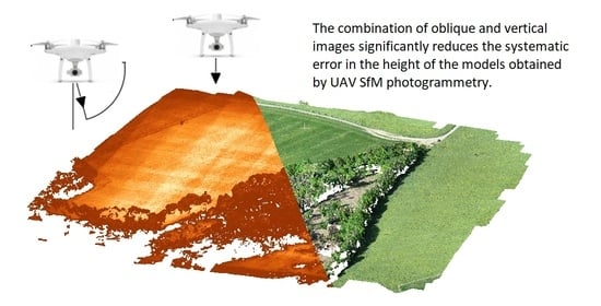
:Georeferencing using ground control points (GCPs) is the most common strategy in photogrammetry modeling using unmanned aerial vehicle (UAV)-acquired imagery. With the increased availability of UAVs with onboard global navigation satellite system–real-time kinematic (GNSS RTK), georeferencing without GCPs is becoming a promising alternative. However, systematic elevation error remains a problem with this technique. We aimed to analyze the reasons for this systematic error and propose strategies for its elimination. Multiple flights differing in the flight altitude and image acquisition axis were performed at two real-world sites. A flight height of 100 m with a vertical (nadiral) image acquisition axis was considered primary, supplemented with flight altitudes of 75 m and 125 m with a vertical image acquisition axis and two flights at 100 m with oblique image acquisition axes (30° and 15°). Each of these flights was performed twice to produce a full double grid. Models were reconstructed from individual flights and their combinations. The elevation error from individual flights or even combinations yielded systematic elevation errors of up to several decimeters. This error was linearly dependent on the deviation of the focal length from the reference value. A combination of two flights at the same altitude (with nadiral and oblique image acquisition) was capable of reducing the systematic elevation error to less than 0.03 m. This study is the first to demonstrate the linear dependence between the systematic elevation error of the models based only on the onboard GNSS RTK data and the deviation in the determined internal orientation parameters (focal length). In addition, we have shown that a combination of two flights with different image acquisition axes can eliminate this systematic error even in real-world conditions and that georeferencing without GCPs is, therefore, a feasible alternative to the use of GCPs.
1. Introduction
UAV photogrammetry combined with the structure from motion (SfM) technique is a well-established method for the mapping and creation of digital terrain models (DTMs), digital elevation models (DEMs), and/or other spatial models. This technique is often used in mining [1,2,3], for monitoring of various natural phenomena and geohazards [4,5], for the detection of agricultural crops/trees [6,7,8], dam and riverbed erosion [9], modeling topographic features [10], updating cadastral data [11], solar irradiation estimates [12], etc. SfM has become so popular that it is currently also used besides ground and UAV photogrammetry in mobile measurement systems [13]; even attempts at creating DTMs using a mobile phone have been reported [14,15,16]. UAV photogrammetry simplifies the work, makes it faster, and improves the quality, although the resulting model accuracy depends on many circumstances, such as the configuration and number of ground control points (GCPs) [17,18], camera pitch [19,20], image overlap [21], flight trajectory [22], camera calibration method [23,24], software used for reconstruction [25], or the quality of global navigation satellite system (GNSS) signal processing [26,27,28]. As well as the point cloud, other outputs, such as orthomosaics, are also widely used [29]. Photogrammetry outcomes are usually evaluated using independent laser scanning or control points (CPs), the position of which is measured by ground surveys, which facilitate the assessment of model deformations [30,31,32]. Correct determination of the elements of internal and external orientation, traditionally performed using GCPs, is crucial for creating an accurate photogrammetric model. At present, the use of UAVs equipped with an onboard global navigation satellite system–real-time kinematic (GNSS RTK) receiver is on the rise. This equipment used to be prohibitively expensive but, lately, it has become more affordable. DJI Phantom 4 RTK multicopter is an example of such a low-end UAV. The knowledge of the camera position during image acquisition (with centimeter accuracy) has been suggested to be able to fully substitute the presence of GCPs for georeferencing of the photogrammetric model [33]. Elimination of the need for GCPs would be a great advantage, potentially making the measurement simpler and/or cheaper; in inaccessible areas, it could be crucial for even making the measurement possible. The resulting model accuracy should correspond to that of the GNSS RTK; the standard deviation should, therefore, not exceed several centimeters. Many studies (e.g., [33]) used such an approach, with satisfactory results. Other studies, however, reported that this approach, combined with the calculation of internal orientation elements when solving bundle adjustment, i.e., without a known camera calibration, yields results systematically shifted in the elevation axis that may be, in some instances, significantly higher than the expected accuracy [34,35,36]. The expected accuracy of the resulting point cloud is 1–2x the ground sampling distance (GSD) [37]; nevertheless, in our previous research, the systematic error was as high as tens of centimeters despite a ground sampling distance (GSD) of 0.03 m [34]. Similar results were presented, for example, by Forlani et al. [38]. The association of such high inaccuracy with the incorrect determination of the focal length (f) was suggested in those studies. Additionally, the systematic error was shown to be more or less random as it differed even between repeated flights on the same site with the same conditions (the same UAV and processed in the same way) [34]. A small number of GCPs [39], or even a single one [34], was, however, shown to significantly reduce this problem. Several studies also suggested methods that should suppress or even remove this phenomenon. Besides the aforementioned use of a minimum number of GCPs, the use of oblique images is another promising alternative [20,36,40]. The presented study aims to propose and test strategies enabling the acquisition of a quality photogrammetric model without the high systematic elevation error while avoiding the use of GCPs. Proof that the source of the error indeed lies in the incorrect focal length determination would show the path to resolving this problem—choosing a flight configuration ensuring a sufficiently accurate calculation of internal orientation elements. We performed image acquisition at two study sites with various flight parameters to independently evaluate the results associated with different external conditions. By processing this acquired imagery in various combinations, we aimed to find a working strategy (configuration) for safe and accurate use of the GNSS RTK-based approach without the systematic elevation error.
2. Materials and Methods
2.1. Data Acquisition
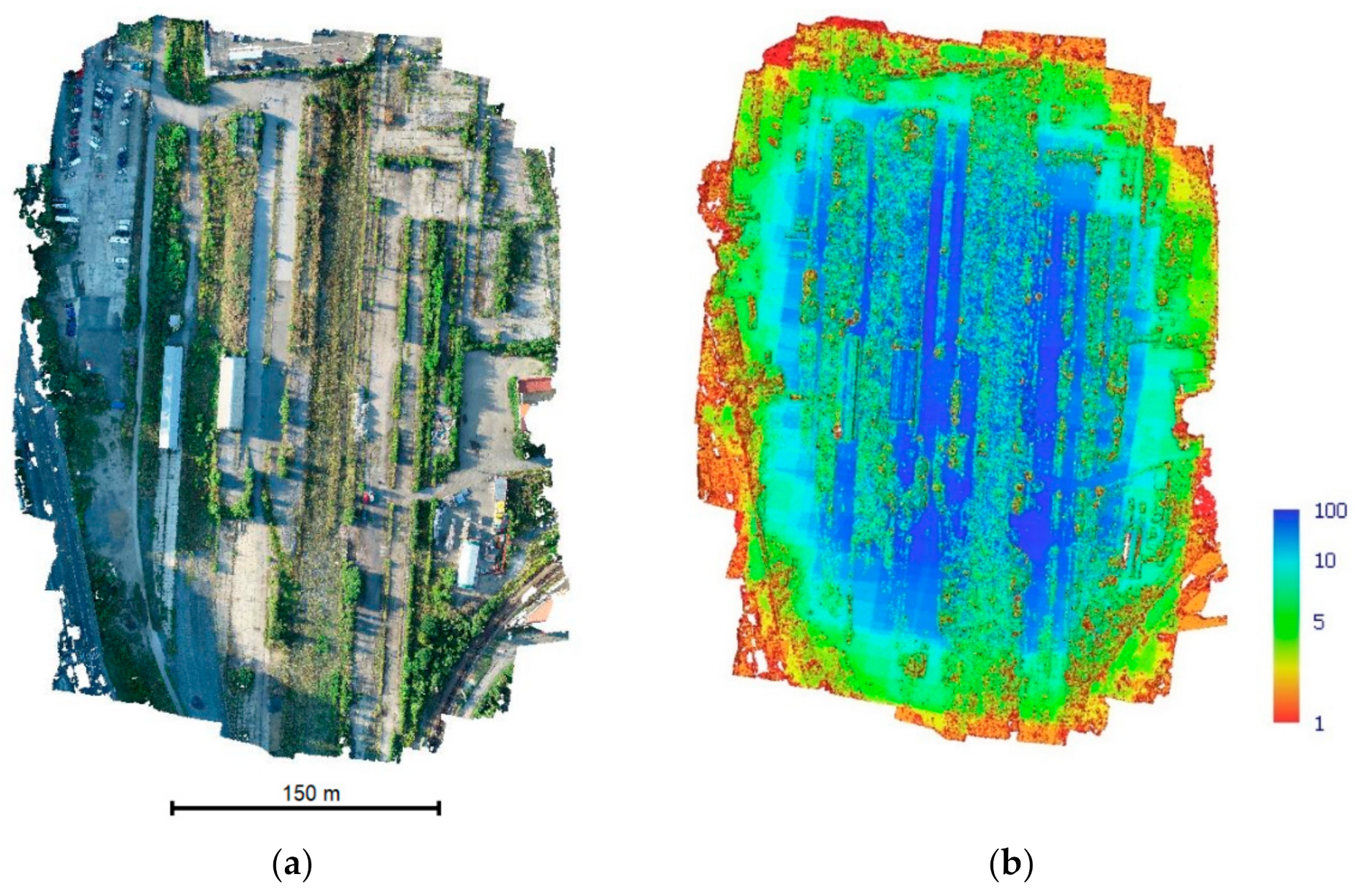
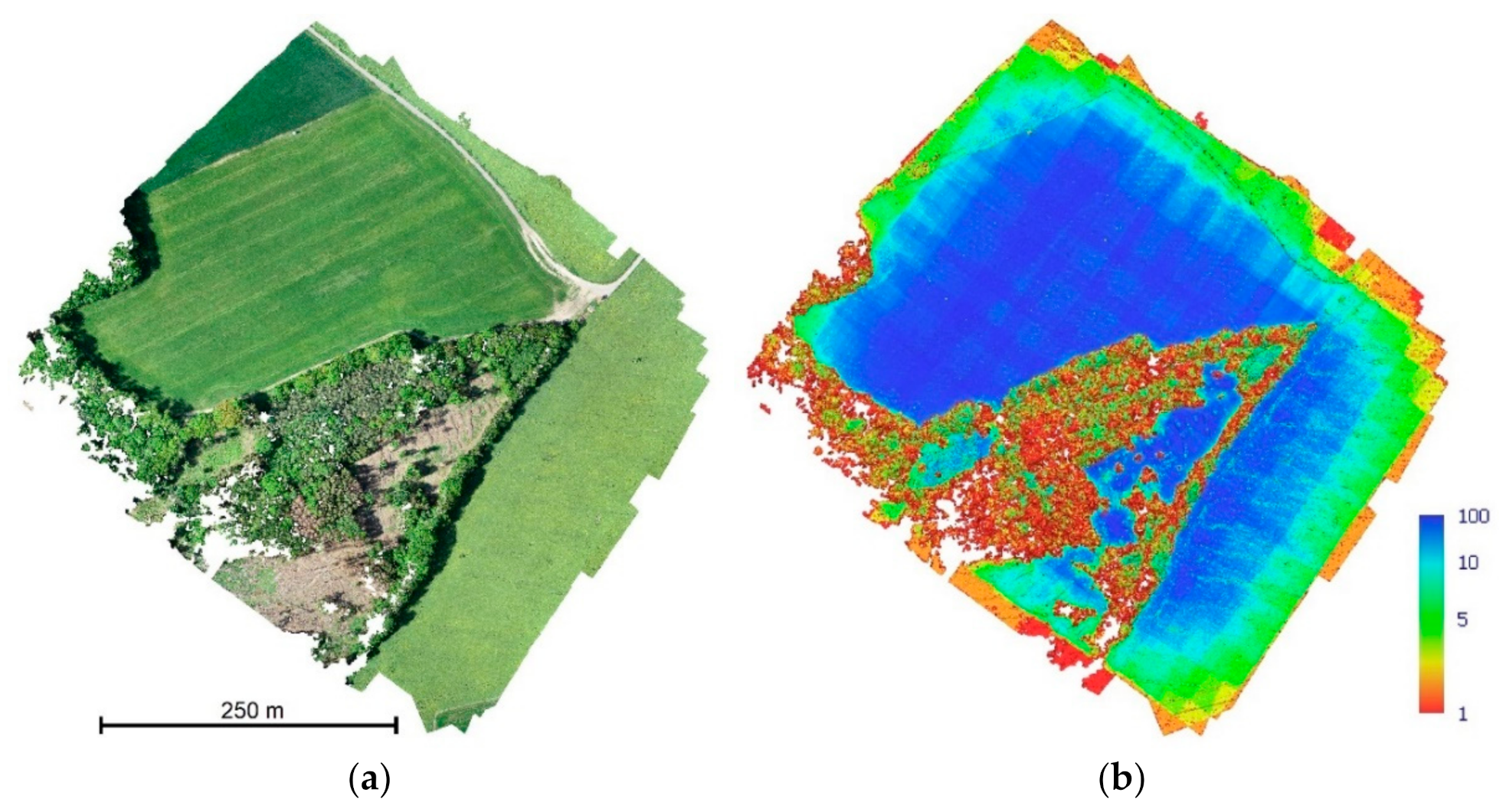
To facilitate the generalization of the results of this study, the experiment was performed in two study sites. The first site—Brownfield—had only a minimum of dense undergrowth, with low buildings, and concrete and natural surfaces without monochromatic areas (Figure 1). The other site—Rural—was characterized by continuous rapeseed fields alternating with more or less dense forest and shrubs (Figure 2). These two sites differ with respect to the present surfaces and their properties. Figure 1 and Figure 2 show the point clouds in colors indicating the reliability of the individual points acquired through SfM in Agisoft Metashape (confidence), with lower numbers indicating lower reliability (confidence; possible range 1–255). The Brownfield site can be, therefore, considered highly suitable for SfM modeling, while the Rural site can be considered problematic, which is particularly true for the part of the site that is covered by dense tree vegetation.
The DJI Phantom 4 RTK UAV mounted with a camera equipped with an FC6310R lens (f = 8.8 mm), resolution of 4864 × 3648 pixels, and with a pixel size of 2.61 × 2.61 μm (total price approx. EUR 6000), was used for image acquisition. The GNSS RTK receiver was connected to the CZEPOS permanent reference station network.
The primary flight altitude was set to 100 m above ground with a vertical image acquisition axis and ground sampling distance (GSD) of 0.03 m; at the same altitude, flights with the image acquisition axis angled by 15° and 30° from the vertical direction were performed. In addition, flights at altitudes of 75 m and 125 m above ground with a nadiral imagery acquisition axis were performed (Figure 3).
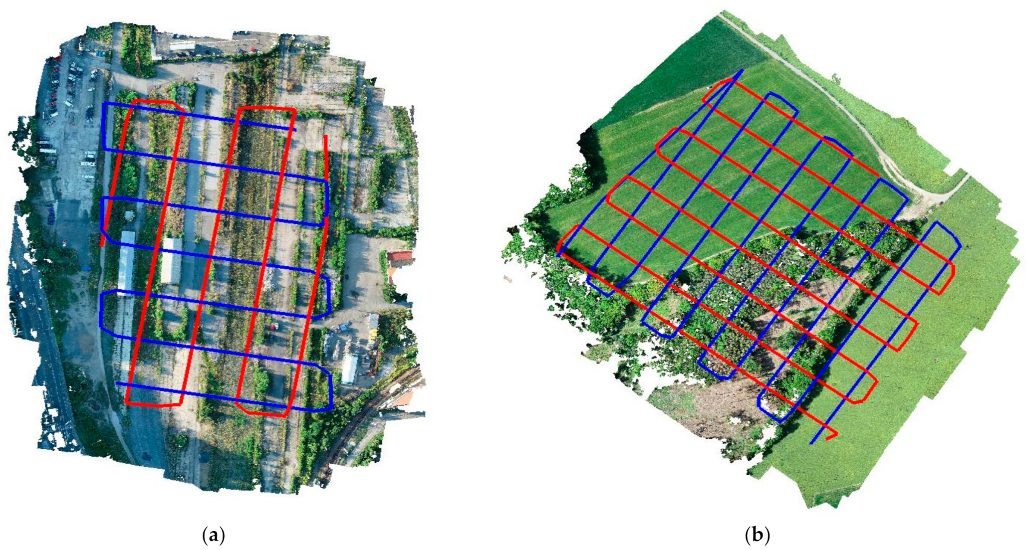
Each flight was performed with a gridded flight plan; two perpendicular flights were performed for each flight setup (forming a double grid, see Figure 4).
Altogether, 10 flights with 75% front and side overlaps were performed. Table 1 shows the parameters of individual flights with the hereinafter used designations and numbers of usable images.
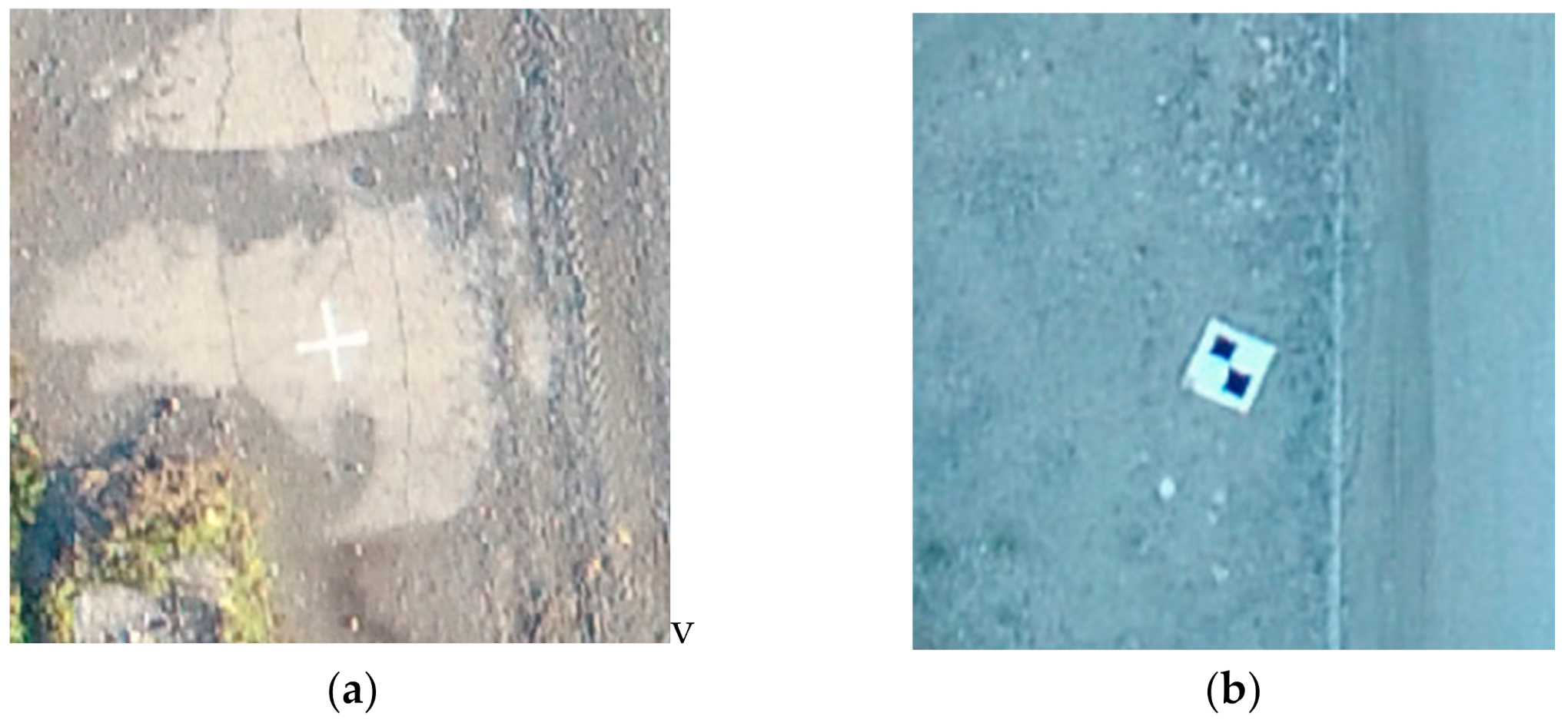
Points that subsequently served, depending on the calculation method, as either control points or ground control points were stabilized at each of the sites. Where possible, these were marked out as a cross painted with a contrast matte spray (Figure 5 left). Where this was not possible, especially in the undergrowth, wooden boards with black and white targets were used (Figure 5, right) and stabilized using a 10 cm long nail. The dimensions of the crosses/targets were approx. 0.40 m × 0.40 m.
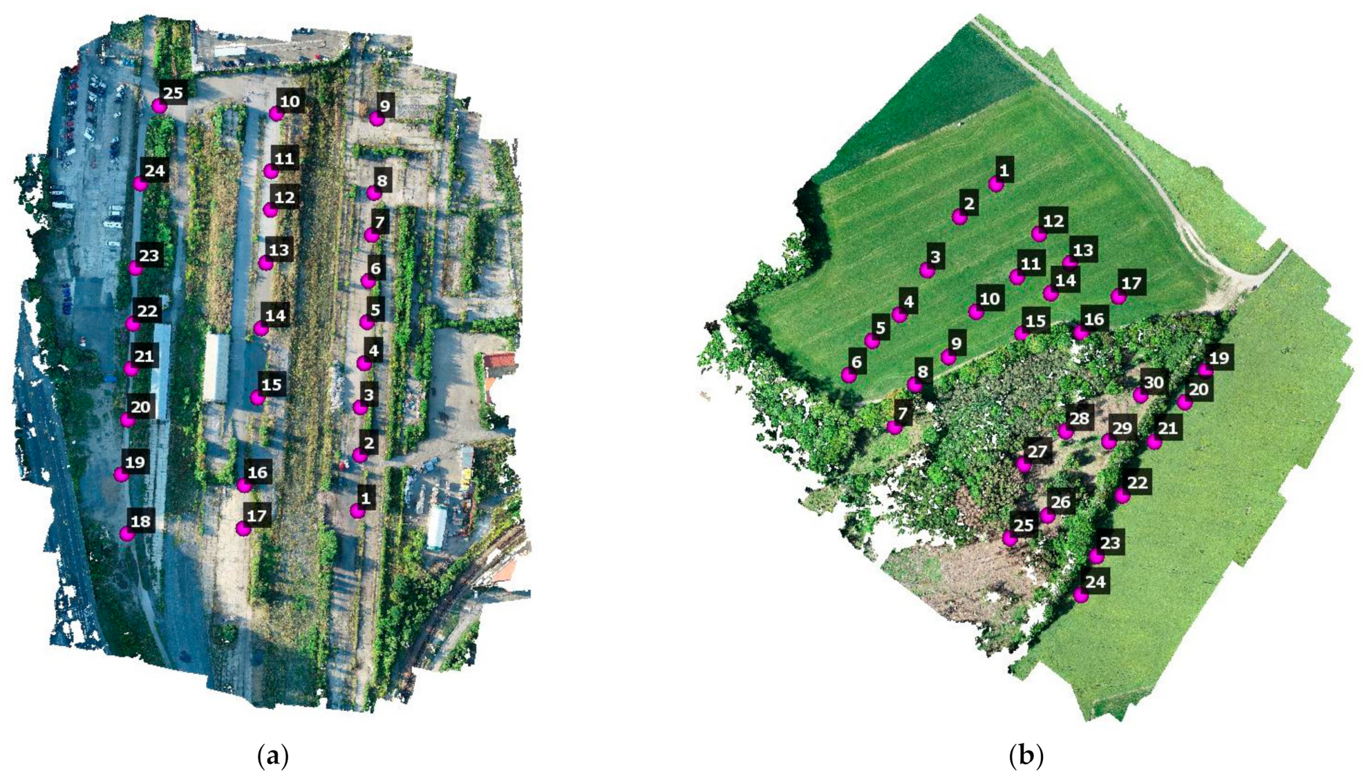
(Ground) control points were distributed as evenly as possible throughout both areas. In all, 25 points were stabilized at the Brownfield site and 30 at the Rural site (Figure 6). The (ground) control points were surveyed using a GNSS RTK Trimble Geo XR receiver with a Zephyr 2 antenna connected into the CZEPOS permanent reference station network (czepos.cuzk.cz). Measurement of each control point was taken three times (before, between, and after UAV flights) for detecting potential errors or variations caused, e.g., by the change of the configuration or satellite availability. The expected nominal accuracy of each coordinate was 0.03 m.
2.2. Data Processing
Both GNSS RTK measurements (UAV onboard and ground receiver) were processed using the same methods. First, the terrestrial GNSS RTK measurements were exported from the receiver in the WGS 84 coordinate system (latitude, longitude, ellipsoidal height). Similarly, the spatial position (in the same coordinate system) was extracted from the GNSS RTK data-containing images using Exiftool. The offset between the GNSS receiver antenna reference point (ARP) and the camera center (CC) was automatically considered by the software. Subsequently, all data were converted into the Czech national coordinate positioning system (S-JTSK, System of Unified Trigonometric Cadastral Network) and the Bpv vertical datum (Balt after adjustment) using the EasyTransform software (http://adjustsolutions.cz/easytransform/, accessed on 1 March 2021) to ensure that the same algorithm was used on all data and thereby to eliminate potential systematic errors that could occur as a result of different transformation algorithms. The three measurements taken for each point by the terrestrial GNSS RTK receiver were used for the calculation of the standard deviation. Then, images were processed in Agisoft Metashape 1.6.1 using the structure from motion calculation method (SfM) with the custom settings listed in Table 2.
The UAV was not equipped with a professional metric camera. Although pre-calibration is generally recommended, the stability of the parameters in non-metric UAV-mounted cameras cannot be fully ascertained and other studies have shown that laboratory calibration does not provide better results than the method used in this study [41,42]. The interior orientation parameters were, therefore, calculated in the usual way.
In all, five duplicate flights were performed at each site. The geometries of the imagery from individual flights differed (the bundles intersected at different points due to different flight altitudes and/or camera angles). Each flight (i.e., 10 flights at each site) was processed separately. In addition, joint processing of the two duplicate flights was also performed (i.e., 5 for each site), which allowed investigation of whether a simple increase in the number of images can improve the accuracy.
The primary flight was at an altitude of 100 m with nadiral image acquisition; the remaining flights were performed to acquire data for testing possible accuracy improvement strategies. Hence, all possible combinations of the 100 m altitude flight with nadiral image acquisition (the primary flight) and flights with other configurations were calculated, i.e.,: 100m_1 + 75m_1; 100m_1 + 125m_1; 100m_1 + 60°_1; 100m_1 + 75°_1; 100m_1 + 75m_2; 100m_1 + 125m_2; 100m_1 + 60°_2; 100m_1 + 75°_2; the same was done for the second primary flight (100m_2). Therefore, 16 such combinations were calculated for each site.
Each of the variants described above was calculated with onboard GNSS RTK data only (All_RTK) and with a combination of the onboard GNSS RTK receiver data with GCP coordinates (All_Combined).
The processing sequence was the same in all flights—alignment, sparse cloud computation, system optimization, dense cloud calculation. Dense cloud was subsequently manually cropped along the convex envelope of GCPs and filtered in CloudCompare 2.11.0 using the CSF filter to remove trees and shrubs that could potentially cause uncertainty in comparisons of the dense clouds.
Subsequently, parameters of the regression and coefficient of determination describing the relationship between the difference in the focal length f (acquired from the respective flight and from all available data from the respective site, i.e., the All_Combined calculation variant) and the (mean) systematic error in the entire model elevation were calculated for each site. Similarly, the correlation between the systematic error in model elevation and the principal point offset difference (Cx, Cy) was also calculated. The aim was to show the association between the elevation error and the calculation of internal orientation elements.
3. Results
3.1. The Accuracy of the GNSS RTK Ground Geodetic Survey
The accuracy of the GCP/checkpoints survey was evaluated through a calculation of standard deviations in individual coordinates SX, SY, SH from the replicates detailed in Table 3. The results confirm the expected accuracy of 0.03 m in each coordinate.
3.2. Elevation Errors and Related Parameters
As shown, e.g., in our previous study [34], the elevation component of the resulting model is the most problematic one when using direct georeferencing based only on onboard GNSS RTK measurements. Therefore, the mean difference in elevation of the control points between the onboard GNSS RTK and the geodetic survey was calculated to obtain the systematic error (Table 4 and Table 5). The residual error was then characterized by the standard deviation, the total error is described by the root mean square error (RMS). Similarly, residual systematic error between the recorded and adjusted camera elevations was calculated for the camera coordinates; the mean difference for individual flights was always equal to zero, and the standard deviation did not exceed 0.03 m (approx. 1x GSD), which confirms that the coordinates recorded during flights were correct. Table 4 and Table 5 also detail other parameters, including the focal length f and the coordinates of the principal point offset Cx and Cy. The first two rows of each table represent the reference values calculated from all images using all available images together with the measured GCP coordinates (All_Combined) and using GNSS RTK coordinates only (All_RTK).
These results indicate that systematic (average) elevation error in individual flights is highly variable, with values as high as 0.85 m in some flights (Brownfield 75° (100 m)−1). It is also apparent that even results derived from two flights at the same height and with the same image acquisition angle differ (both between sites and within the same site). The standard deviation of elevation is approximately 0.03 m, which is in accordance with the expected GNSS RTK measurement accuracy.
The All_Combined variants demonstrate a very good agreement of all measured images and coordinates, i.e., that no outliers or erroneous measurements are present. The agreement of internal orientation elements is also very good (a bit worse between sites).
It should be also noted that a higher systematic elevation error was observed in flights where a higher difference between the focal length f calculated for the particular flight and the most likely value determined from the All_Combined calculation occurred. Similar conclusions can be made with respect to the coordinates of the principal point offset.
Table 6 and Table 7 show the results of calculations performed using both corresponding flights. Obviously, the increase in the number of images from the two mutually perpendicular flights led to a reduction of the systematic (mean) elevation error, which is particularly true for the Brownfield site. However, it still exceeds the expected measurement accuracy.
Table 8 and Table 9 detail the values of combined calculations. It is obvious that in the Brownfield site, basically any non-homogeneous combination of flight parameters improved the results to such a degree that the maximum mean elevation error did not exceed 0.05 m and the total error (RMS) of 0.053 m, which is still less than two GSDs. On the other hand, no such improvement was observed when data from flights performed at two different heights were combined at the Rural site; the systematic error still remained up to 0.4 m. However, the combination of the flight at 100 m and flights with oblique image acquisition improved the systematic errors; the improvement increased when increasing the image acquisition angle from the nadiral direction. The standard deviations are similar in all these cases, approximately 0.03 m.
3.3. Analysis of the Association between the Systematic Error in Elevation and the Deviation of the Focal Length f
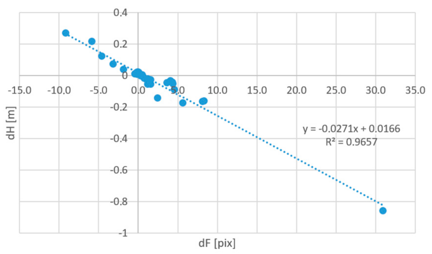
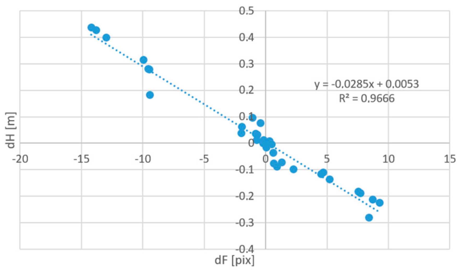
The data detailed in Table 4, Table 5, Table 6, Table 7, Table 8, and Table 9 were used for the calculation of the differences between the determined focal lengths and the reference value determined from the All-Combined calculation variant. The relationship is shown in Figure 7 and Figure 8, along with the regression coefficients and determination coefficient (calculated in MS Excel).
Both the graphical record and the determination coefficient R2, which is in both cases close to 1 (0.97), prove a practically linear association of the systematic error and the focal length error, which confirms the hypothesis stated, for example, in our previous paper [34].
The linear regression parameters can be further interpreted. The constant element represents the independent constant error (mutual difference) between coordinates determined by the onboard UAV GNSS RTK receiver and the terrestrial GNSS RTK survey. The detected size of the difference (max 0.017 m) corresponds to the declared accuracy of 0.03 m. The line direction can also be interpreted; using triangle similarity, the following simple equation can be derived:
describing the geometric configuration of the regression line direction as h/f, where h is the flight altitude above the terrain and f is the focal length. The primary flight altitude in the performed experiments was always h = 100 m and the focal length f = 3685 pix, the ratio h/f was therefore 0.027 m/pix, which is very close to the experimentally determined h/f values (0.0271 for the Brownfield site and −0.0285 for the Rural site).
The practically linear relationship between the constant chamber deviation and the systematic error in elevation proves that the inaccuracy of the internal orientation element calculation is indeed the source of that error. The focal length f determined during model calculation can, therefore, be used as an indicator of this error.
A similar approach to the calculation of the correlation coefficient was also applied to the coordinates of the principal point offset Cx and Cy. However, in this case, no reasonable correlation was found; there is, therefore, no direct relationship between the erroneous computation of the principal point offset and the systematic elevation error.
3.4. Comparison of Dense Clouds
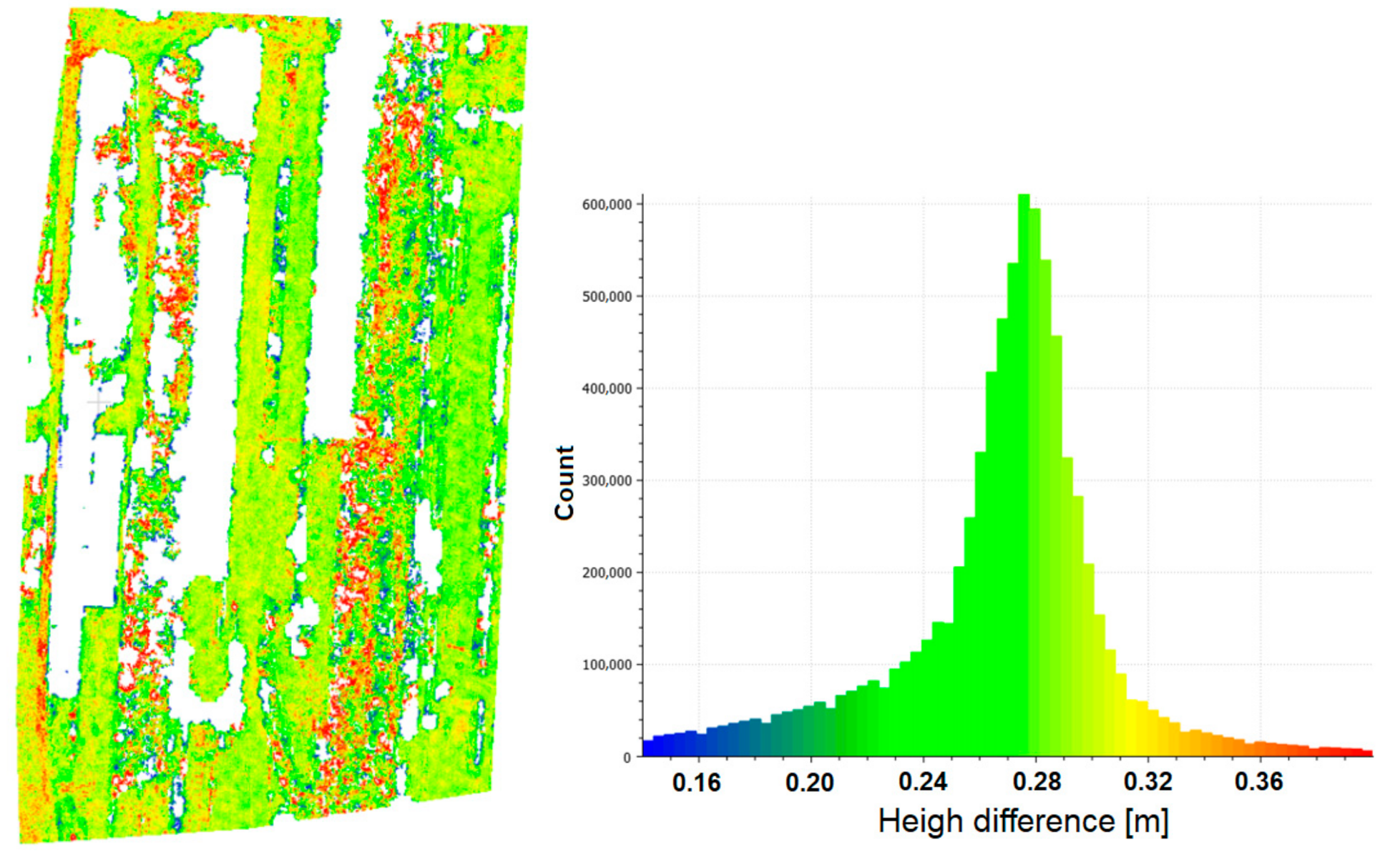
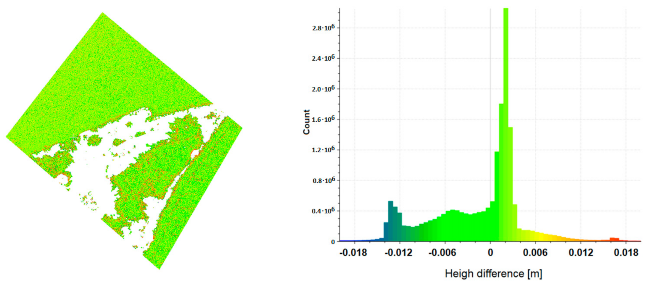
Thus far, all comparisons and evaluations in this paper were performed using control points (CPs) in CloudCompare software. It is, therefore, necessary to show that this acquired information also has general validity, i.e., that it is also valid for the generated dense cloud point. For this purpose, the data were cropped, filtered to remove trees and shrubs, and the resulting cloud points were compared. The data from All_Combined calculations (utilizing all available data) were, again, used as the reference. Below, results of the comparisons of the All_Combined calculations to calculations from the primary flight providing the worse result from each location are shown. The comparison of the point clouds from the 100 m−1 flight and All_Combined dataset for Brownfield returned a systematic elevation error of 0.268 m with a standard deviation of elevation of 0.038 m, as illustrated by Figure 9. This systematic shift corresponds very well to the value calculated from control points (see Table 4). The comparison of the All_Combined data and 100m_2 flight for the Rural site illustrated in Figure 10 revealed a systematic error of 0.305 m with a standard deviation of 0.029 m. Again, this systematic shift corresponds very well to the value obtained from the control points (0.315 m; see Table 5). The last presented comparison focused on the difference between All_Combined and All_RTK point clouds, which demonstrates the practical agreement of the resulting point clouds; it is obvious that no deformation has occurred and the elevation difference is practically constant (the systematic shift is 0.002 m and the standard deviation is 0.006 m).
The comparisons of the point cloud elevations to the All_Combined variant detailed in Figure 9, Figure 10 and Figure 11 clearly show that the average difference value corresponds to that calculated using control points, and the same can be said about the standard deviation. The results of analyses of the remaining point clouds were in agreement with this statement, which proves that the difference is indeed caused by a systematic shift of the point cloud in the nadiral direction without deformation in the horizontal plane.
It is also obvious that the All_RTK and All_Combined calculation variants produced practically identical results, which implies that if the internal orientation elements are determined correctly, the result is correct even if only onboard RTK data are used.
4. Discussion
Many studies have tested the use of UAV photogrammetry with onboard GNSS RTK for preparing a point cloud representing a DTM and subsequent calculations. Although, in principle, it is possible to perform the whole calculation without the use of GCPs, practical testing revealed that simultaneous calculation of the internal and external orientation elements may, in some cases, lead to a systematic elevation error, although all measurements are correct. This elevation error is random in a way, as it differed even in duplicate flights with the same configuration and the same UAV. This is in accordance with the findings by other authors (e.g., [34,36,38,39]), regardless of whether a fixed-wing or rotary-wing UAV was used.
James and Robson described in 2014 a so-called doming effect when creating a photogrammetric model solely from photographs without the use of reference points. This was not observed in our paper, which can be explained by the fact that the current algorithms used in Agisoft Metashape already consider the camera coordinates during construction of the model [43].
A detailed analysis of the results revealed that incorrect calculation of the internal orientation elements, particularly of the focal length f, is the most likely reason for this problem (e.g., [34,38,40]). Various strategies to deal with this problem have been proposed, such as the use of oblique images (e.g., [19,36,40]), including a small number of GCPs (e.g., [36,39,40,44]) or camera pre-calibration (e.g., [34,42]). Disregarding the use of GCPs (a reliable solution which, however, negates the principal goal of this study, i.e., the simplification of the measurement by avoiding the use of GCPs), it is necessary to try to propose a measurement strategy (flight configuration, processing method, other techniques) to prevent the systematic error. In this study, we aimed to prove the association between the systematic elevation error and erroneous determination of the internal orientation elements and to test various strategies for eliminating the systematic elevation error. We have shown experimentally in two sites (33 models calculated at each site) that the systematic error in elevation and deviation of the focal length are practically linearly dependent, with a coefficient of determination of more than 0.96. The regression coefficients also correspond very well to the relationship between the flight altitude and focal length (Equation (1)). This implies that it is necessary to adopt a strategy ensuring the best possible determination of the internal orientation elements. Here, we must also note that the correct camera calibration is indeed a principal problem of photogrammetry. There are methods that can be used for this purpose, but they usually rely on the use of GCPs and a very specific image acquisition configuration. Additionally, it is also well known that pre/post-calibration, i.e., calibration independent of the particular flight, brings (when using UAVs with non-metric cameras) poorer results than the calibration performed within the scope of the particular flight [45]. It is, therefore, necessary to choose approaches that are actually feasible from the perspective of the camera mounted on the UAV and that can be simply implemented in the image acquisition flight. Here, we combined the primary flight (100 m altitude, nadiral image acquisition) with imagery acquired from other flights. The results of the evaluation of such combined calculations revealed that:
- Performing duplicate flights, even if the second flight is perpendicular to the first one (double-grid), brings only a minor improvement; however, the accuracy still remains above the expected limit of 1–2 GSD. In some cases, it may still fail with a systematic shift of up to 0.18 m.
- Geometrically different combinations (i.e., the primary flight combined with flights at other altitudes or with different camera angles) led to a significant improvement. This was especially apparent at the Brownfield site where any of these combinations led to the expected accuracy (elevation difference below 0.05 m). Still, the error at the Rural site remained in some instances as high as 0.4 m. It is, therefore, obvious that the quality and selection of the key points for image matching affect the quality of the calibration.
- The best results were obtained from the combinations of the primary flight and flights with oblique image acquisition. This was the only strategy that worked well at both sites in all tested combinations. The variant with the higher angle (30° from the vertical direction) provided the best results, with even the worst systematic error not exceeding 0.03 m (1 GSD).
In our experiment, only relatively small camera angles (15° and 30° from the vertical direction) were used to prevent disruption of image alignment, which could pose problems in rugged terrain (i.e., terrain with sloped surfaces). Obviously, the higher the difference in the camera angle, the greater are the differences between the appearance of the same area in the images and, therefore, the more difficult the image matching. Some studies [36,40] used a greater angle (45°) but these were performed on an “ideal” flat terrain. The possible angles and their effect on the resulting accuracy should be subject to further research.
5. Conclusions
UAVs equipped with onboard GNSS RTK receivers are becoming financially more accessible. Their usage for SfM modeling without the need for GCPs seems to be a natural path to take; however, the usual flight configuration with nadiral image acquisition and self-calibration often produces results with significant systematic elevation error. In this study, we have proved that the principal cause for this is the incorrect determination of the internal orientation parameters as the resulting elevation error is practically directly proportional to the error in the determination of the focal length (coefficient of determination of 0.96). This was also confirmed by the numerical agreement with the geometrical relationship.
To be able to use an onboard GNSS RTK receiver for direct georeferencing, it is, therefore, necessary to ensure correct calibration of the internal orientation elements; where the use of GCPs and/or accurate camera calibration is not possible or feasible, the results can be improved by adjusting the flight geometry and calculation method. We have tested strategies of joint calculations of two flights that were (i) geometrically identical and (ii) geometrically different. A major difference was revealed between sites; at the site with surfaces suitable for SfM, all tested non-homogeneous flight combinations yielded satisfactory results and the systematic error was reduced to approx. 1 GSD; on the contrary, at the Rural site, covered predominantly with rapeseed, shrubs, trees, and other vegetation, combining different flight altitudes did not result in sufficient improvement. However, combinations of two flights at the same altitude with different camera acquisition axes (nadiral and oblique) performed very well. The combination with the higher difference in acquisition angle (i.e., of nadiral and 30 deg from nadiral image acquisition axes) performed best, capable of reducing the systematic elevation error to approx. 1 GSD even in the Rural area with a surface highly unsuitable for photogrammetry.
Author Contributions
Conceptualization: M.Š.; methodology: M.Š.; ground data acquisition: T.R. and J.S.; UAV data acquisition: J.B.; data processing of UAV imagery: T.R. and J.S.; analysis and interpretation of results: M.Š. and R.U.; manuscript drafting: M.Š. and R.U. All authors have read and agreed to the published version of the manuscript.
Funding
This research was funded by the Grant Agency of CTU in Prague—grant number SGS21/053/OHK1/1T/11 “Optimization of acquisition and processing of 3D data for purpose of engineering surveying, geodesy in underground spaces and 3D scanning”.
Institutional Review Board Statement
Not applicable.
Informed Consent Statement
Not applicable.
Data Availability Statement
Not applicable.
Conflicts of Interest
The authors declare no conflict of interest. The funders had no role in the design of the study; in the collection, analyses, or interpretation of data; in the writing of the manuscript, or in the decision to publish the results.
References
- Park, S.; Choi, Y. Applications of Unmanned Aerial Vehicles in Mining from Exploration to Reclamation: A Review. Minerals 2020, 10, 663. [Google Scholar] [CrossRef]
- Kršák, B.; Blišťan, P.; Pauliková, A.; Puškárová, P.; Kovanič, L.; Palková, J.; Zelizňaková, V. Use of low-cost UAV photogrammetry to analyze the accuracy of a digital elevation model in a case study. Meas. J. Int. Meas. Confed. 2016, 91, 276–287. [Google Scholar] [CrossRef]
- Blistan, P.; Jacko, S.; Kovanič, Ľ.; Kondela, J.; Pukanská, K.; Bartoš, K. TLS and SfM Approach for Bulk Density Determination of Excavated Heterogeneous Raw Materials. Minerals 2020, 10, 174. [Google Scholar] [CrossRef] [Green Version]
- Pavelka, K.; Šedina, J.; Matoušková, E.; Hlaváčová, I.; Korth, W. Examples of different techniques for glaciers motion monitoring using InSAR and RPAS. Eur. J. Remote Sens. 2019, 5, 219–232, ISSN 2279-7254. [Google Scholar] [CrossRef] [Green Version]
- Kovanič, Ľ.; Blistan, P.; Urban, R.; Štroner, M.; Blišťanová, M.; Bartoš, K.; Pukanská, K. Analysis of the Suitability of High-Resolution DEM Obtained Using ALS and UAS (SfM) for the Identification of Changes and Monitoring the Development of Selected Geohazards in the Alpine Environment—A Case Study in High Tatras, Slovakia. Remote Sens. 2020, 12, 3901. [Google Scholar] [CrossRef]
- Komárek, J.; Klouček, T.; Prošek, J. The potential of Unmanned Aerial Systems: A tool towards precision classification of hard-to-distinguish vegetation types? Int. J. Appl. Earth Obs. Geoinf. 2018, 71, 9–19. [Google Scholar] [CrossRef]
- Klouček, T.; Komárek, J.; Surový, P.; Hrach, K.; Janata, P.; Vašíček, B. The Use of UAV Mounted Sensors for Precise Detection of Bark Beetle Infestation. Remote Sens. 2019, 11, 1561. [Google Scholar] [CrossRef] [Green Version]
- Šedina, J.; Housarová, E.; Raeva, P. Using of rpas in precision agriculture. In 17th International Multidisciplinary Scientific Geoconference, Conference Proceedings Volume 17, Informatics, Geoinformatics and Remote Sensing Issue 22, Geodesy and Mine Surveying. Sofia: International Multidisciplinary Scientific GeoConference SGEM; STEF92 Technology Ltd.: Sofia, Bulgaria, 2017; Volume 17, pp. 331–338, ISSN 1314-2704; ISBN 978-619-7408-02-7. [Google Scholar] [CrossRef]
- Buffi, G.; Manciola, P.; Grassi, S.; Barberini, M.; Gambi, A. Survey of the Ridracoli Dam: UAV–based photogrammetry and traditional topographic techniques in the inspection of vertical structures. Geomat. Nat. Hazards Risk 2017, 8, 1562–1579. [Google Scholar] [CrossRef] [Green Version]
- Kumhálová, J.; Moudrý, V. Topographical characteristics for precision agriculture in conditions of the Czech Republic. Appl. Geogr. 2014, 50, 90–98. [Google Scholar] [CrossRef]
- Puniach, E.; Bieda, A.; C´wia˛kała, P.; Kwartnik-Pruc, A.; Parzych, P. Use of Unmanned Aerial Vehicles (UAVs) for Updating Farmland Cadastral Data in Areas Subject to Landslides. ISPRS Int. J. Geo-Inf. 2018, 7, 331. [Google Scholar] [CrossRef] [Green Version]
- Moudrý, V.; Beková, A.; Lagner, O. Evaluation of a high resolution UAV imagery model for rooftop solar irradiation estimates. Remote Sens. Lett. 2019, 10, 1077–1085. [Google Scholar] [CrossRef]
- Kalvoda, P.; Nosek, J.; Kuruc, M.; Volařík, T.; Kalvodova, P. Accuracy Evaluation and Comparison of Mobile Laser Scanning and Mobile Photogrammetry Data; IOP Conference Series: Earth and Environmental Science; IOP Publishing Ltd.: Bristol, UK, 2020; pp. 1–10, ISSN 1755-1307. [Google Scholar] [CrossRef]
- Tavani, S.; Pignalosa, A.; Corradetti, A.; Mercuri, M.; Smeraglia, L.; Riccardi, U.; Seers, T.; Pavlis, T.; Billi, A. Photogrammetric 3D Model via Smartphone GNSS Sensor: Workflow, Error Estimate, and Best Practices. Remote Sens. 2020, 12, 3613. [Google Scholar] [CrossRef]
- Tavani, S.; Corradetti, A.; Granado, P.; Snidero, M.; Seers, T.D.; Mazzoli, S. Smartphone: An alternative to ground control points for orienting virtual outcrop models and assessing their quality. Geosphere 2019, 15, 2043–2052. [Google Scholar] [CrossRef]
- Jaud, M.; Bertin, S.; Beauverger, M.; Augereau, E.; Delacourt, C. RTK GNSS-Assisted Terrestrial SfM Photogrammetry without GCP: Application to Coastal Morphodynamics Monitoring. Remote Sens. 2020, 12, 1889. [Google Scholar] [CrossRef]
- Sanz-Ablanedo, E.; Chandler, J.H.; Rodríguez-Pérez, J.R.; Ordóñez, C. Accuracy of Unmanned Aerial Vehicle (UAV) and SfM Photogrammetry Survey as a Function of the Number and Location of Ground Control Points Used. Remote Sens. 2018, 10, 1606. [Google Scholar] [CrossRef] [Green Version]
- Agüera-Vega, F.; Carvajal-Ramírez, F.; Martínez-Carricondo, P. Assessment of photogrammetric mapping accuracy based on variation ground control points number using unmanned aerial vehicle. Measurement 2017, 98, 221–227. [Google Scholar] [CrossRef]
- Vacca, G.; Dessì, A.; Sacco, A. The Use of Nadir and Oblique UAV Images for Building Knowledge. ISPRS Int. J. Geo-Inf. 2017, 6, 393. [Google Scholar] [CrossRef] [Green Version]
- Nesbit, P.R.; Hugenholtz, C.H. Enhancing UAV–SfM 3D Model Accuracy in High-Relief Landscapes by Incorporating Oblique Images. Remote Sens. 2019, 11, 239. [Google Scholar] [CrossRef] [Green Version]
- Gerke, M.; Nex, F.; Remondino, F.; Jacobsen, K.; Kremer, J.; Karel, W.; Hu, H.; Ostrowski, W. Orientation of oblique airborne image sets–experiences from the isprs/eurosdr benchmark on multi-platform photogrammetry. Int. Arch. Photogramm. Remote Sens. Spatial Inf. Sci. 2016, 41, 185–191. [Google Scholar] [CrossRef] [Green Version]
- Gerke, M.; Przybilla, H.J. Accuracy Analysis of Photogrammetric UAV Image Blocks: Influence of Onboard RTK-GNSS and Cross Flight Patterns. Photogramm. Fernerkund. Geoinf. 2016, 2016, 17–30. [Google Scholar] [CrossRef] [Green Version]
- Forlani, G.; Diotri, F.; Morra di Cella, U.; Roncella, R. UAV Block GEOREFERENCING and control by on-board GNSS data. Int. Arch. Photogramm. Remote Sens. Spatial Inf. Sci 2020, XLIII-B2-2020, 9–16. [Google Scholar] [CrossRef]
- Jon, J.; Koska, B.; Pospíšil, J. Autonomous Airship Equipped with Multi-Sensor Mapping Platform. ISPRS-Int. Arch. Photogramm. Remote Sens. Spat. Inf. Sci. 2013, 40, 119–124, ISSN 2194-9034. [Google Scholar] [CrossRef] [Green Version]
- Jaud, M.; Passot, S.; Le Bivic, R.; Delacourt, C.; Grandjean, P.; Le Dantec, N. Assessing the Accuracy of High Resolution Digital Surface Models Computed by PhotoScan® and MicMac® in Sub-Optimal Survey Conditions. Remote Sens. 2016, 8, 465. [Google Scholar] [CrossRef] [Green Version]
- Tahar, K.N.; Kamarudin, S.S. Uav onboard gps in positioning determination. Int. Arch. Photogramm. Remote Sens. Spatial Inf. Sci. 2016, XLI-B1, 1037–1042. [Google Scholar] [CrossRef] [Green Version]
- Urban, R.; Štroner, M.; Kuric, I. The use of onboard UAV GNSS navigation data for area and volume calculation. Acta Montan. Slovaca 2020, 25, 361–374. [Google Scholar] [CrossRef]
- Padró, J.C.; Munoz, F.J.; Planas, J.; Pons, X. Comparison of four UAV georeferencing methods for environmental monitoring purposes focusing on the combined use with airborne and satellite remote sensing platforms. Int. J. Appl. Earth Obs. Geoinf. 2019, 75, 130–140. [Google Scholar] [CrossRef]
- Hung, I.-K.; Unger, D.; Kulhavy, D.; Zhang, Y. Positional Precision Analysis of Orthomosaics Derived from Drone Captured Aerial Imagery. Drones 2019, 3, 46. [Google Scholar] [CrossRef] [Green Version]
- Křemen, T. Measurement and Documentation of St. Spirit Church in Liběchov. In Advances and Trends in Geodesy, Cartography and Geoinformatics II; Taylor & Francis Group: London, UK, 2020; pp. 44–49. ISBN 978-0-367-34651-5. [Google Scholar] [CrossRef]
- Koska, B.; Křemen, T. The Combination of Laser Scanning and Structure from Motion Technology for Creation of Accurate Exterior and Interior Orthophotos of St. Nicholas Baroque Church. ISPRS Int. Arch. Photogramm. Remote Sens. Spat. Inf. Sci. 2013, XL-5/W1, 133–138, ISSN 2194-9034. [Google Scholar] [CrossRef] [Green Version]
- Moudrý, V.; Lecours, V.; Gdulová, K.; Gábor, L.; Moudrá, L.; Kropáček, J.; Wild, J. On the use of global DEMs in ecological modelling and the accuracy of new bare-earth DEMs. Ecol. Model. 2018, 383, 3–9, ISSN 0304-3800. [Google Scholar] [CrossRef]
- Tomaštík, J.; Mokroš, M.; Surový, P.; Grznárová, A.; Merganič, J. UAV RTK/PPK Method—An Optimal Solution for Mapping Inaccessible Forested Areas? Remote Sens. 2019, 11, 721. [Google Scholar] [CrossRef] [Green Version]
- Štroner, M.; Urban, R.; Reindl, T.; Seidl, J.; Brouček, J. Evaluation of the Georeferencing Accuracy of a Photogrammetric Model Using a Quadrocopter with Onboard GNSS RTK. Sensors 2020, 20, 2318. [Google Scholar] [CrossRef] [PubMed] [Green Version]
- Peppa, M.V.; Hall, J.; Goodyear, J.; Mills, J.P. Photogrammetric Assessment and Comparison of DJI Phantom 4 Pro and Phantom 4 RTK Small Unmanned Aircraft Systems. Int. Arch. Photogramm. Remote Sens. Spat. Inf. Sci 2019, XLII-2/W13, 503–509. [Google Scholar] [CrossRef] [Green Version]
- Taddia, Y.; Stecchi, F.; Pellegrinelli, A. Coastal Mapping using DJI Phantom 4 RTK in Post-Processing Kinematic Mode. Drones 2020, 4, 9. [Google Scholar] [CrossRef] [Green Version]
- Santise, M.; Fornari, M.; Forlani, G.; Roncella, R. Evaluation of DEM generation accuracy from UAS imagery. Int. Arch. Photogramm. Remote Sens. Spatial Inf. Sci. 2014, XL-5, 529–536. [Google Scholar] [CrossRef] [Green Version]
- Forlani, G.; Dall’Asta, E.; Diotri, F.; Cella, U.M.; Roncella, R.; Santise, M. Quality Assessment of DSMs Produced from UAV Flights Georeferenced with On-Board RTK Positioning. Remote Sens. 2018, 10, 311. [Google Scholar] [CrossRef] [Green Version]
- Le Van Canh, X.; Cao Xuan Cuong, X.; Nguyen Quoc Long, X.; Le Thi Thu Ha, X.; Tran Trung Anh, X.; Xuan-Nam Bui, X. Experimental Investigation on the Performance of DJI Phantom 4 RTK in the PPK Mode for 3D Mapping Open-Pit Mines. Inz. Miner. J. Pol. Miner. Eng. Soc. 2020, 46, 65–74, ISSN 1640-4920. [Google Scholar] [CrossRef]
- Teppati Losè, L.; Chiabrando, F.; Giulio Tonolo, F. Boosting the Timeliness of UAV Large Scale Mapping. Direct Georeferencing Approaches: Operational Strategies and Best Practices. ISPRS Int. J. Geo-Inf. 2020, 9, 578. [Google Scholar] [CrossRef]
- Cramer, M.; Przybilla, H.-J.; Zurhorst, A. UAV cameras: Overview and geometric calibration benchmark. Int. Arch. Photogramm. Remote Sens. Spatial Inf. Sci. 2017, XLII-2/W6, 85–92. [Google Scholar] [CrossRef] [Green Version]
- Harwin, S.; Lucieer, A.; Osborn, J. The Impact of the Calibration Method on the Accuracy of Point Clouds Derived Using Unmanned Aerial Vehicle Multi-View Stereopsis. Remote Sens. 2015, 7, 11933–11953. [Google Scholar] [CrossRef] [Green Version]
- James, M.R.; Robson, S. Mitigating systematic error in topographic models derived from UAV and ground-based image networks. Earth Surf. Proc. Landf. 2014, 39, 1413–1420. [Google Scholar] [CrossRef] [Green Version]
- Zhang, H.; Aldana-Jague, E.; Clapuyt, F.; Wilken, F.; Vanacker, V.; Van Oost, K. Evaluating the potential of post-processing kinematic (PPK) georeferencing for UAV-based structure- from-motion (SfM) photogrammetry and surface change detection. Earth Surf. Dynam. 2019, 7, 807–827. [Google Scholar] [CrossRef] [Green Version]
- Przybilla, H.-J.; Bäumker, M.; Luhmann, T.; Hastedt, H.; Eilers, M. Interaction between direct georeferencing, control point configuration and camera self-calibration for rtk-based uav photogrammetry. Int. Arch. Photogramm. Remote Sens. Spatial Inf. Sci. 2020, 43, 485–492. [Google Scholar] [CrossRef]
Figure 1.
Brownfield site ((a) orthomosaic, (b) point cloud color-coded according to confidence).

Figure 2.
Rural site ((a) orthomosaic, (b) point cloud color-coded according to confidence).

Figure 3.
Flight altitudes and image acquisition directions.

Figure 4.
Flight trajectory: (a) Brownfield; (b) Rural. Flight 1 in red, Flight 2 in blue.

Figure 5.
(Ground) control points; (a) marking using a spray; (b) using black and white target.

Figure 6.
Distribution of the (ground) control points throughout the study sites—Brownfield (a), Rural (b).
Figure 6.
Distribution of the (ground) control points throughout the study sites—Brownfield (a), Rural (b).

Figure 7.
The systematic error of elevation as a function of the deviation of the focal length f from the reference value—Brownfields).
Figure 7.
The systematic error of elevation as a function of the deviation of the focal length f from the reference value—Brownfields).

Figure 8.
The systematic error of elevation as a function of the deviation of the focal length f from the reference value—Rural.
Figure 8.
The systematic error of elevation as a function of the deviation of the focal length f from the reference value—Rural.

Figure 9.
Height differences between 100m_1 RTK and All_Combined point clouds—Brownfield (area cropped along outer control points).
Figure 9.
Height differences between 100m_1 RTK and All_Combined point clouds—Brownfield (area cropped along outer control points).

Figure 10.
Comparison of All_Combined to the worst result of individual flights, i.e., the flight 100m_2—Rural (area cropped along outer control points).
Figure 10.
Comparison of All_Combined to the worst result of individual flights, i.e., the flight 100m_2—Rural (area cropped along outer control points).

Figure 11.
Comparison of All_RTK to All_Combined —Rural.


Table 1.
Image acquisition flights and their properties.
| Site | Designation | Flight Altitude above the Terrain (m) | Imagery Acquisition—Deviation from the Nadiral Direction (°) | Number of Images—Flight 1 | Number of Images—Flight 2 |
|---|---|---|---|---|---|
| Brownfield | 75 m | 75 | 0 | 78 | 76 |
| 100 m | 100 | 0 | 50 | 53 | |
| 125 m | 125 | 0 | 39 | 41 | |
| 60° (100 m) | 100 | 30 | 67 | 80 | |
| 75° (100 m) | 100 | 15 | 58 | 66 | |
| Rural | 75 m | 75 | 0 | 176 | 183 |
| 100 m | 100 | 0 | 112 | 122 | |
| 125 m | 125 | 0 | 84 | 84 | |
| 60° (100 m) | 100 | 30 | 147 | 160 | |
| 75° (100 m) | 100 | 15 | 128 | 140 |
Table 2.
Agisoft Metashape settings used for calculations.
| Setting | Value |
|---|---|
| Align Photos | |
| -Accuracy | High |
| -Key point limit | 40,000 |
| -Tie point limit | 4000 |
| Optimize Camera Alignment | Fit all constants (f, cx, cy, k1–k4, p1–p4) |
| Build Dense Cloud | |
| -Quality | High |
| -Depth filtering | Moderate |
| Digital Elevation Model | |
| -Coordinate System | S-JTSK, Bpv |
| -Parameters | |
| -Source data | Dense Cloud |
| -Interpolation | Enabled |
| -Advanced | |
| -Resolution | 2.8 cm/pix (implicit) |
| (Settings not detailed above were kept at default). | |
Table 3.
Agisoft Metashape settings used for calculations.
| Site | SX (m) | SY (m) | SH (m) | S in 3D Position (m) |
|---|---|---|---|---|
| Rural | 0.0063 | 0.0046 | 0.0069 | 0.010 |
| Brownfield | 0.0061 | 0.0051 | 0.0067 | 0.010 |
Table 4.
Results of calculation variants—individual flights—Brownfield.
| Calculation Variant | Mean Difference (m) | StDev (m) | RMS (m) | f (Pixels) | Cx (Pixels) | Cy (Pixels) |
|---|---|---|---|---|---|---|
| All_Combined | 0.0201 | 0.0063 | 0.0211 | 3685.4568 | 9.9062 | 28.3165 |
| All_RTK | 0.0254 | 0.0063 | 0.0261 | 3685.3472 | 9.9037 | 28.3546 |
| 75m_1 | 0.0412 | 0.0080 | 0.0419 | 3683.5605 | 9.5506 | 27.7429 |
| 75m_2 | 0.0769 | 0.0107 | 0.0776 | 3682.2500 | 9.5145 | 27.7860 |
| 100m_1 | 0.2715 | 0.0115 | 0.2717 | 3676.2500 | 9.8893 | 27.4269 |
| 100m_2 | 0.1252 | 0.0104 | 0.1256 | 3680.7900 | 9.3435 | 27.6945 |
| 125m_1 | −0.1701 | 0.0225 | 0.1716 | 3691.0449 | 9.8862 | 27.5684 |
| 125m_2 | 0.2200 | 0.0153 | 0.2205 | 3679.5466 | 9.5863 | 27.7279 |
| 60° (100m)_1 | −0.1398 | 0.0093 | 0.1401 | 3687.8589 | 9.6792 | 22.6777 |
| 60° (100m)_2 | −0.0541 | 0.0100 | 0.0550 | 3687.0000 | 9.5963 | 25.4033 |
| 75° (100m)_1 | −0.8557 | 0.0115 | 0.8558 | 3716.3172 | 12.1673 | 13.5000 |
| 75° (100m)_2 | −0.1610 | 0.0113 | 0.1613 | 3693.5500 | 11.0213 | 26.6421 |
Table 5.
Results of calculation variants—individual flights—Rural.
| Calculation Variant | Mean (m) | StDev (m) | RMS (m) | f (Pixels) | Cx (Pixels) | Cy (Pixels) |
|---|---|---|---|---|---|---|
| All_Combined | −0.0126 | 0.0237 | 0.0265 | 3685.1506 | 9.0573 | 29.2059 |
| All_RTK | −0.0145 | 0.0241 | 0.0278 | 3685.1948 | 9.0573 | 29.1926 |
| 75m_1 | −0.1813 | 0.0211 | 0.1825 | 3692.6899 | 9.4703 | 27.8337 |
| 75m_2 | 0.1829 | 0.0376 | 0.1866 | 3675.7142 | 8.9789 | 30.0060 |
| 100m_1 | 0.0369 | 0.0243 | 0.0440 | 3684.3132 | 9.5869 | 30.4881 |
| 100m_2 | 0.3154 | 0.0318 | 0.3170 | 3675.1982 | 9.4326 | 30.2998 |
| 125m_1 | −0.0755 | 0.0231 | 0.0789 | 3685.7920 | 8.2727 | 27.9129 |
| 125m_2 | 0.4000 | 0.0238 | 0.4007 | 3672.1744 | 8.1549 | 28.0104 |
| 60° (100m)_1 | −0.0971 | 0.0297 | 0.1014 | 3687.4122 | 9.9673 | 24.2402 |
| 60° (100m)_2 | 0.0761 | 0.0274 | 0.0807 | 3684.7123 | 8.3047 | 31.9379 |
| 75° (100m)_1 | −0.2793 | 0.0403 | 0.2821 | 3693.5554 | 9.6960 | 23.1674 |
| 75° (100m)_2 | −0.0715 | 0.0315 | 0.0780 | 3686.4340 | 9.0964 | 29.4237 |
Table 6.
Results of calculation variants: joint calculation of duplicate flights—Brownfield.
| Calculation Variant | Mean (m) | StDev (m) | RMS (m) | F (Pixels) | Cx (Pixels) | Cy (Pixels) |
|---|---|---|---|---|---|---|
| All_Combined | 0.0201 | 0.0063 | 0.0211 | 3685.4568 | 9.9062 | 28.3165 |
| 75m_1 + 75m_2 | −0.0869 | 0.0080 | 0.0873 | 3690.0200 | 9.6071 | 28.0833 |
| 100m_1 + 100m_2 | 0.0089 | 0.0070 | 0.0112 | 3685.3100 | 9.6407 | 27.9082 |
| 125m_1 + 125m_2 | 0.0217 | 0.0142 | 0.0257 | 3685.2400 | 9.7382 | 27.7874 |
| 60°_1 + 60°_2 (100m) | −0.0517 | 0.0073 | 0.0522 | 3686.6200 | 9.4244 | 25.6123 |
| 75°_1 + 75°_2 (100m) | −0.1596 | 0.0104 | 0.1600 | 3693.7200 | 11.1567 | 26.3864 |
Table 7.
Results of calculation variants: joint calculation of duplicate flights—Rural.
| Calculation Variant | Mean (m) | StDev (m) | RMS (m) | F (Pixels) | Cx (Pixels) | Cy (Pixels) |
|---|---|---|---|---|---|---|
| All_Combined | −0.0126 | 0.0237 | 0.0265 | 3685.1506 | 9.0573 | 29.2059 |
| 75m_1 + 75m_2 | −0.1879 | 0.0266 | 0.1897 | 3692.8619 | 9.2088 | 29.2684 |
| 100m_1 + 100m_2 | −0.1088 | 0.0253 | 0.1116 | 3689.8473 | 9.4996 | 30.5776 |
| 125m_1 + 125m_2 | −0.0865 | 0.0215 | 0.0890 | 3686.0700 | 8.3529 | 28.1841 |
| 60°_1 + 60°_2 (100m) | 0.0962 | 0.0235 | 0.0989 | 3684.0718 | 8.5973 | 31.4189 |
| 75°_1 + 75°_2 (100m) | −0.0343 | 0.0299 | 0.0452 | 3685.7482 | 9.0306 | 28.9058 |
Table 8.
Results of calculation variants: non-homogenous combinations of the flight at 100 m with nadiral axis of image acquisition and other flights—Brownfield.
Table 8.
Results of calculation variants: non-homogenous combinations of the flight at 100 m with nadiral axis of image acquisition and other flights—Brownfield.
| Calculation Variant | Mean (m) | StDev (m) | RMS (m) | F (Pixels) | Cx (Pixels) | Cy (Pixels) |
|---|---|---|---|---|---|---|
| All_Combined | 0.0201 | 0.0063 | 0.0211 | 3685.4568 | 9.9062 | 28.3165 |
| 100m_1 + 75m_1 | −0.0197 | 0.0073 | 0.0210 | 3686.6469 | 9.6673 | 27.8125 |
| 100m_1 + 75m_2 | −0.0246 | 0.0084 | 0.0259 | 3687.0021 | 9.8057 | 27.7864 |
| 100m_2 + 75m_1 | −0.0010 | 0.0074 | 0.0073 | 3685.7385 | 9.4378 | 27.8479 |
| 100m_2 + 75m_2 | −0.0046 | 0.0086 | 0.0096 | 3686.0403 | 9.4761 | 27.9108 |
| 100m_1 + 125m_1 | 0.0012 | 0.0155 | 0.0152 | 3685.9121 | 9.7736 | 27.6163 |
| 100m_1 + 125m_2 | 0.0061 | 0.0105 | 0.0119 | 3685.9438 | 9.8531 | 27.7257 |
| 100m_2 + 125m_1 | −0.0272 | 0.0146 | 0.0308 | 3686.5826 | 9.5823 | 27.8234 |
| 100m_2 + 125m_2 | −0.0141 | 0.0106 | 0.0175 | 3686.1716 | 9.4705 | 27.8232 |
| 100m_1 + 60°_1 | 0.0181 | 0.0079 | 0.0196 | 3685.2030 | 9.8340 | 27.4012 |
| 100m_1 + 60°_2 | 0.0218 | 0.0093 | 0.0237 | 3685.4790 | 9.8563 | 27.5374 |
| 100m_2 + 60°_1 | 0.0137 | 0.0084 | 0.0159 | 3684.9970 | 9.4563 | 27.8556 |
| 100m_2 + 60°_2 | 0.0188 | 0.0078 | 0.0203 | 3685.2289 | 9.4574 | 27.7306 |
| 100m_1 + 75°_1 | −0.0311 | 0.0099 | 0.0326 | 3689.4667 | 10.4964 | 27.9219 |
| 100m_1 + 75°_2 | −0.0409 | 0.0122 | 0.0426 | 3689.7403 | 10.4778 | 28.1390 |
| 100m_2 + 75°_1 | −0.0439 | 0.0079 | 0.0446 | 3689.0670 | 10.2551 | 28.0417 |
| 100m_2 + 75°_2 | −0.0504 | 0.0159 | 0.0527 | 3689.8025 | 10.2318 | 28.2601 |
Table 9.
Results of calculation variants: non-homogenous combinations of the flight at 100 m with nadiral axis of image acquisition and other flights—Rural.
Table 9.
Results of calculation variants: non-homogenous combinations of the flight at 100 m with nadiral axis of image acquisition and other flights—Rural.
| Calculation Variant | Mean (m) | StDev (m) | RMS (m) | F (Pixels) | Cx (Pixels) | Cy (Pixels) |
|---|---|---|---|---|---|---|
| All_Combined | −0.0126 | 0.0237 | 0.0265 | 3685.1506 | 9.0573 | 29.2059 |
| 100m_1 + 75m_1 | −0.1148 | 0.0219 | 0.1168 | 3689.6683 | 9.6098 | 29.3811 |
| 100m_1 + 75m_2 | −0.1343 | 0.0319 | 0.1379 | 3690.3496 | 9.4486 | 30.4642 |
| 100m_2 + 75m_1 | −0.2110 | 0.0246 | 0.2124 | 3693.8792 | 9.5771 | 29.1683 |
| 100m_2 + 75m_2 | −0.2231 | 0.0358 | 0.2258 | 3694.4234 | 9.5165 | 30.2986 |
| 100m_1 + 125m_1 | 0.2818 | 0.0246 | 0.2828 | 3675.5925 | 8.8262 | 29.1363 |
| 100m_1 + 125m_2 | 0.2790 | 0.0238 | 0.2800 | 3675.6822 | 8.9231 | 29.2559 |
| 100m_2 + 125m_1 | 0.4269 | 0.0269 | 0.4277 | 3671.3294 | 8.8258 | 28.9144 |
| 100m_2 + 125m_2 | 0.4379 | 0.0249 | 0.4386 | 3670.9576 | 8.8740 | 29.2264 |
| 100m_1 + 60°_1 | 0.0127 | 0.0251 | 0.0277 | 3684.4032 | 9.5076 | 29.8877 |
| 100m_1 + 60°_2 | −0.0036 | 0.0248 | 0.0246 | 3685.6338 | 9.2217 | 30.2379 |
| 100m_2 + 60°_1 | 0.0334 | 0.0261 | 0.0422 | 3684.4453 | 9.5665 | 29.8517 |
| 100m_2 + 60°_2 | 0.0085 | 0.0264 | 0.0273 | 3685.4680 | 9.3255 | 30.0001 |
| 100m_1 + 75°_1 | 0.0400 | 0.0253 | 0.0471 | 3683.1644 | 9.3780 | 29.8556 |
| 100m_1 + 75°_2 | 0.0010 | 0.0265 | 0.0261 | 3684.9419 | 9.4006 | 30.6061 |
| 100m_2 + 75°_1 | 0.0628 | 0.0266 | 0.0680 | 3683.2049 | 9.3918 | 29.8083 |
| 100m_2 + 75°_2 | 0.0126 | 0.0299 | 0.0320 | 3684.9628 | 9.4726 | 30.3318 |
Publisher’s Note: MDPI stays neutral with regard to jurisdictional claims in published maps and institutional affiliations. |
© 2021 by the authors. Licensee MDPI, Basel, Switzerland. This article is an open access article distributed under the terms and conditions of the Creative Commons Attribution (CC BY) license (https://creativecommons.org/licenses/by/4.0/).
Share and Cite
MDPI and ACS Style
Štroner, M.; Urban, R.; Seidl, J.; Reindl, T.; Brouček, J. Photogrammetry Using UAV-Mounted GNSS RTK: Georeferencing Strategies without GCPs. Remote Sens. 2021, 13, 1336. https://0-doi-org.brum.beds.ac.uk/10.3390/rs13071336
AMA Style
Štroner M, Urban R, Seidl J, Reindl T, Brouček J. Photogrammetry Using UAV-Mounted GNSS RTK: Georeferencing Strategies without GCPs. Remote Sensing. 2021; 13(7):1336. https://0-doi-org.brum.beds.ac.uk/10.3390/rs13071336
Chicago/Turabian StyleŠtroner, Martin, Rudolf Urban, Jan Seidl, Tomáš Reindl, and Josef Brouček. 2021. "Photogrammetry Using UAV-Mounted GNSS RTK: Georeferencing Strategies without GCPs" Remote Sensing 13, no. 7: 1336. https://0-doi-org.brum.beds.ac.uk/10.3390/rs13071336
Note that from the first issue of 2016, this journal uses article numbers instead of page numbers. See further details here.