
Quantifying Understory Complexity in Unmanaged Forests Using TLS and Identifying Some of Its Major Drivers

 , , ,
, , ,
Abstract
: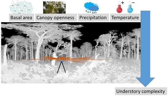
1. Introduction
2. Material and Methods
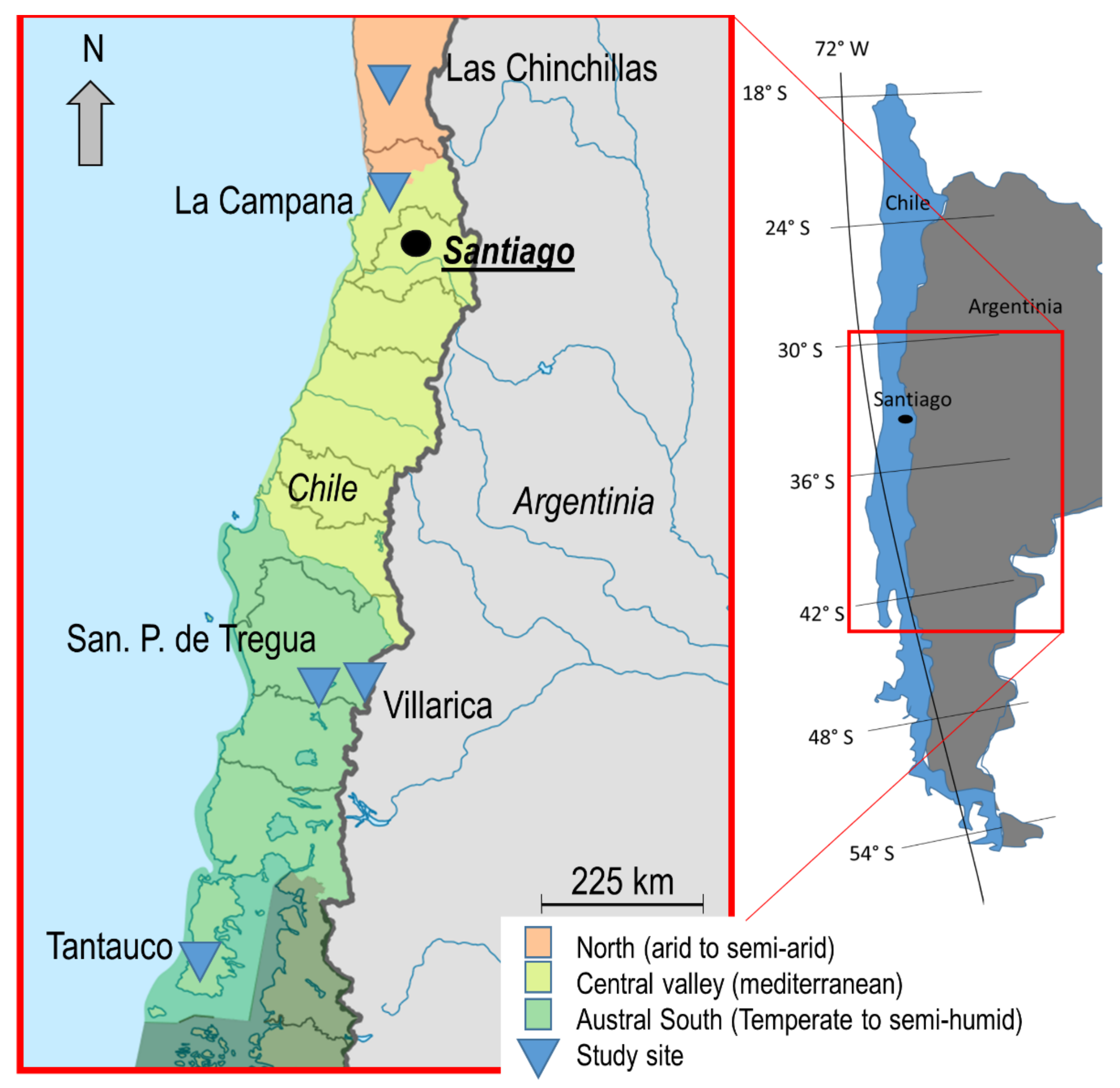
2.1. Study Sites
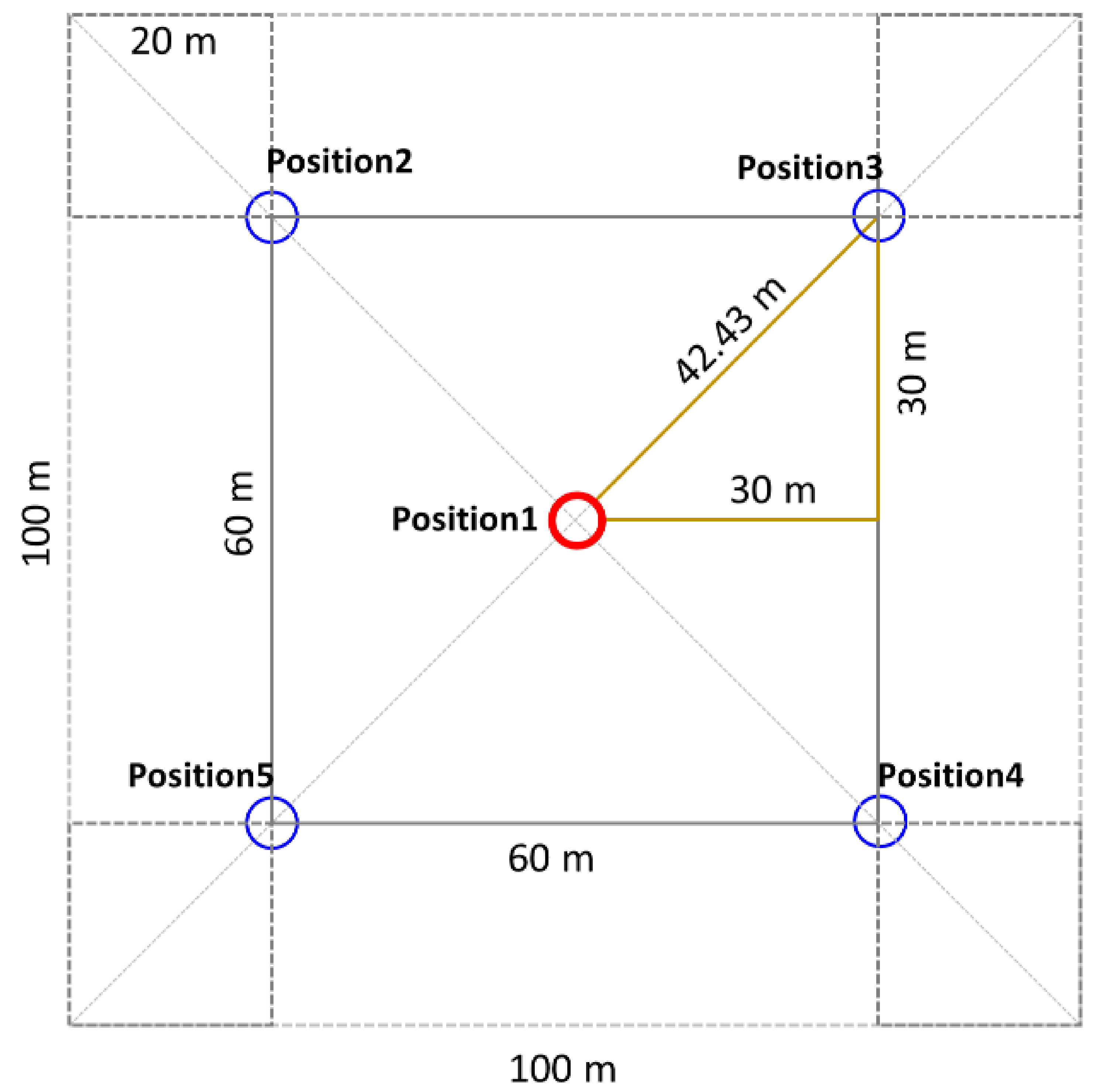
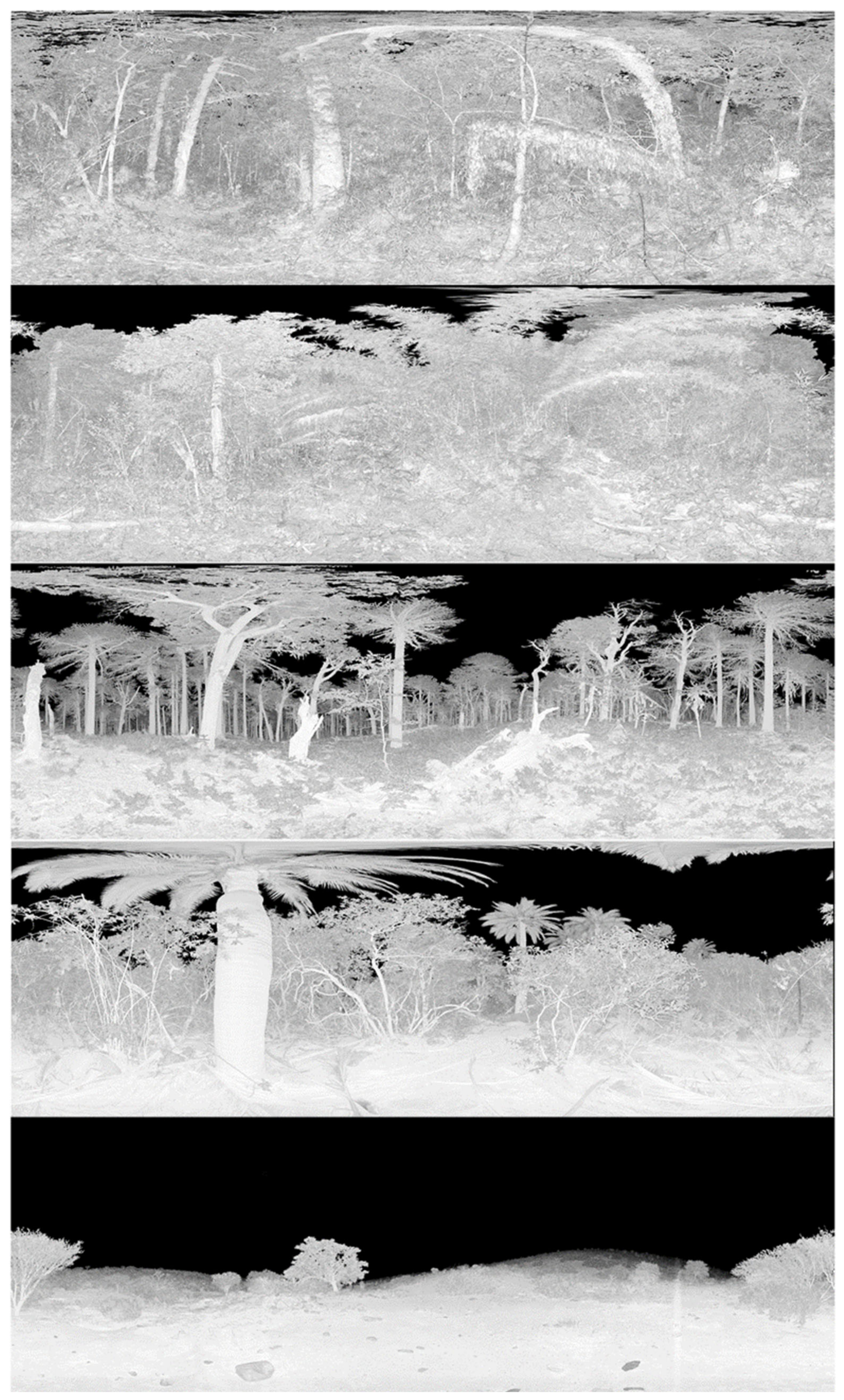
2.2. Sampling Scheme and Scan Settings

| Parque Tantauco | San Pablo de Tregua | Parque N. Villarica | Parque N. la Campana | Reserva Nacional las Chinchillas | |
|---|---|---|---|---|---|
| Abbreviation | Tantauco | San P. de Tregua | Villarica | La Campana | Las Chinchillas |
| Geographical coordinates | 43°1′4″ S 73°47′44″ W | 39°36’14″ S 72°5′43″ W | 39°34′54″ S 71°30′50″ W | 32°56′41″ S 71°4′57″ W | 31°30′28″ S 71°6′39″ W |
| Biogeographic region | South temperate 15 | North temperate 15 | North temperate 15 | South Mediterranean 15 | Central Mediterranean 15 |
| Bedrock | Metamorphic 1 | Volcanic ash 10 | Volcanic ash 11 | Granite 12 | Granite 13 |
| Soil moisture regime | Udic 14 | Udic 14 | Udic 14 | Xeric 14 | Xeric 14 |
| Landscape type | Forest | Forest | Forest | Forest | Shrubland |
| Region | Los Lagos | Los Rios | Araucania | Valparaiso | Coquimbo |
| Province | Chiloé | Valdivia | Cautín | Quillota | Chaopa |
| Nearest City | Quellón | Panguipulli | Curarrehue | Hijuelas | Illapel |
| Founded | 2005 | 1972 | 1940 | 1967 | 1983 |
| Management | Old-growth | Old-growth | Old-growth | Old-growth | Old-growth |
| Status | Private Park | Reserve | National Park | National Park | Reserve |
| Size (ha) | 118.000 | 2.184 | 63.000 | 8.000 | 4.229 |
| Mean annual temperature (°C) (1970–2000) 9 | 9.39 | 8.35 | 6.78 | 14.42 | 14.09 |
| Mean annual precipitation (mm) (1970–2000) 9 | 2295.85 | 2055.43 | 1252.75 | 343.80 | 185.00 |
| Main overstory tree species | ND, NB, DW, AL, SC, LP, PN 1,2,3 | ND, SC, LP 3,4,5 | AA, ND, NA, EC, ND 3,6 | JC, QS, LC, PCH, CA, AC, PB 3,7 | QS, LC, MB, PL, PCH 3,8 |
| Main understory tree species | Bt, Mc, DS, Cv, Lr 1,3 | Bt, Lr, Hi, Cv 3,5 | Pl, Lr, Lq 3 | Ech, Al, Bl, Co 3 | Ech, Al, Bl, Co 3 |
| No. of plots | 9 | 7 | 3 | 4 | 4 |
| No. of scans | 33 * | 35 | 15 | 20 | 20 |
| Mean basal area (m²/ha) | 34.18 | 52.34 | 57.73 | 28.00 | 0.5 |
| Mean canopy openness (%) | 5 | 7 | 30 | 25 | 96 |
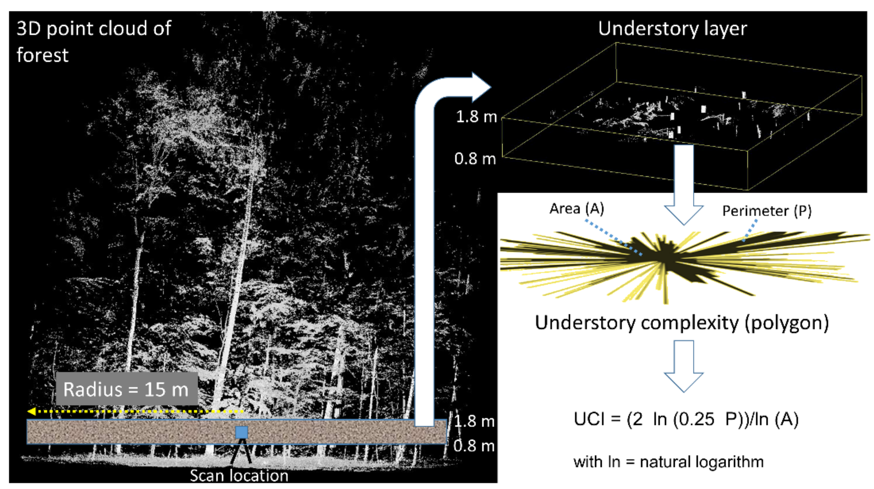
2.3. Calculation of Understory Layer Complexity and Canopy Openness from Laser Scans
2.4. Climate Data
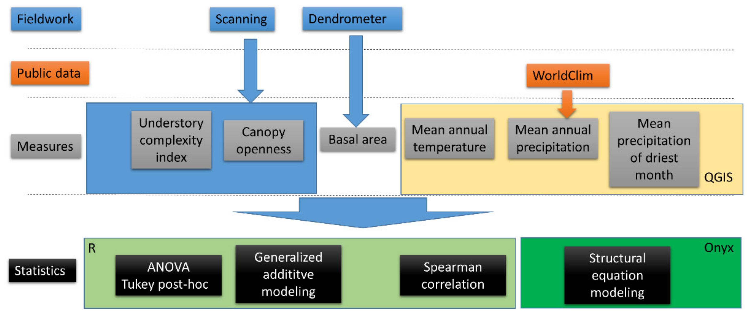
2.5. Statistical Analysis
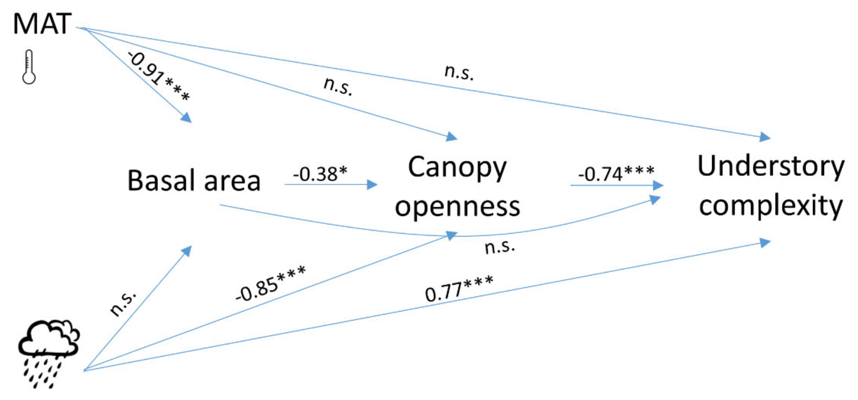
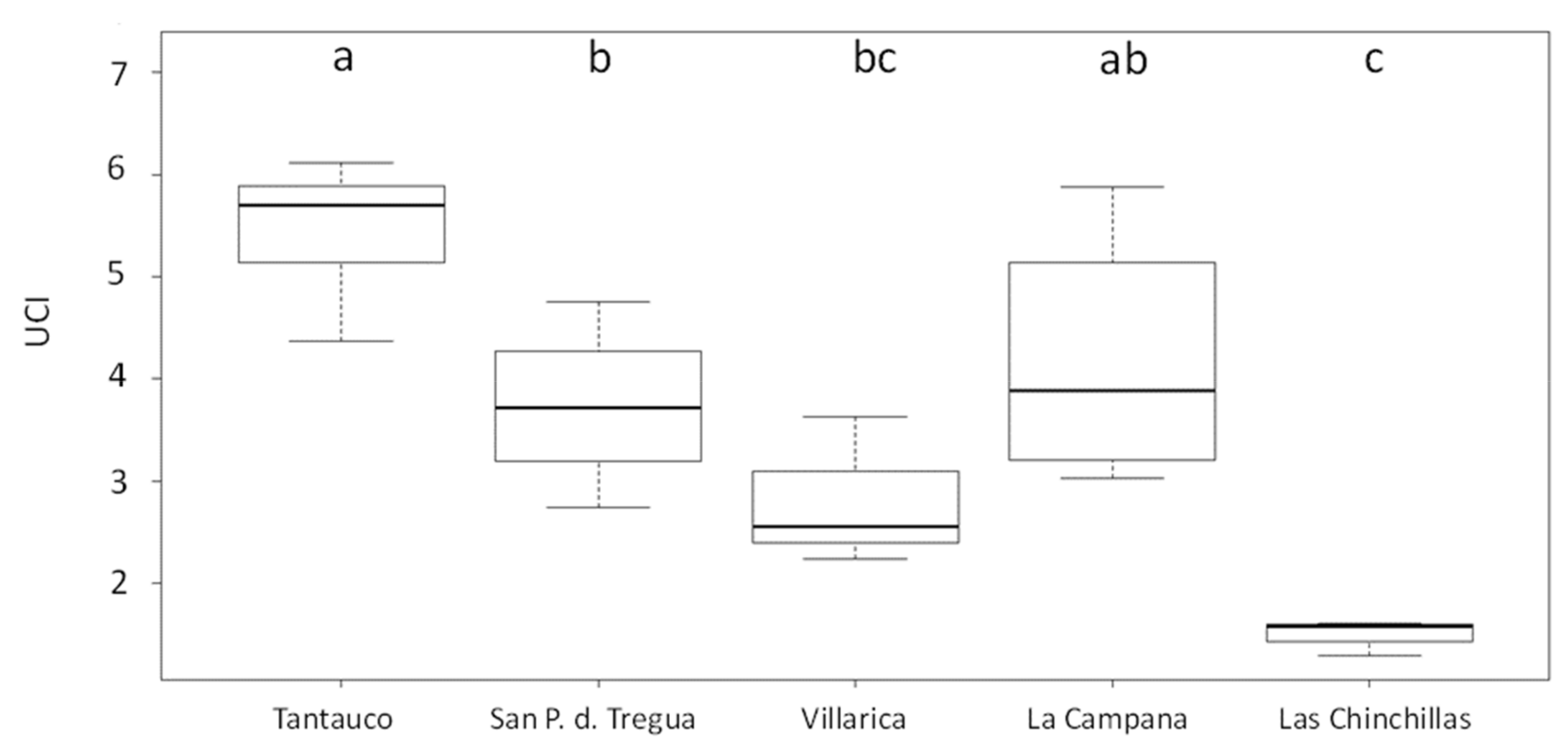
3. Results
4. Discussion
5. Conclusions
Author Contributions
Funding
Institutional Review Board Statement
Informed Consent Statement
Data Availability Statement
Acknowledgments
Conflicts of Interest
References
- Augusto, L.; Dupouey, J.-L.; Ranger, J. Effects of tree species on understory vegetation and environmental conditions in temperate forests. Ann. For. Sci. 2003, 60, 823–831. [Google Scholar] [CrossRef]
- Hartley, M.J. Rationale and methods for conserving biodiversity in plantation forests. For. Ecol. Manag. 2002, 155, 81–95. [Google Scholar] [CrossRef]
- Thomas, S.C.; Halpern, C.B.; Falk, D.A.; Liguori, D.A.; Austin, K.A. Plant diversity in managed forests: Understory responses to thinning and fertilization. Ecol. Appl. 1999, 9, 864–879. [Google Scholar] [CrossRef]
- Kimmins, J.P. The Biogeochemical Cycle: Nutrient Cycling Within Ecosystems. In Forest Ecology: A Foundation for Sustainable Forest Management and Environmental Ethics in Forestry, 3rd ed.; Prentice Hall: Upper Saddle River, NJ, USA, 2004; pp. 103–104. [Google Scholar]
- Eichhorn, M.P.; Ryding, J.; Smith, M.J.; Gill, R.M.; Siriwardena, G.M.; Fuller, R.J. Effects of deer on woodland structure revealed through terrestrial laser scanning. J. Appl. Ecol. 2017, 54, 1615–1626. [Google Scholar] [CrossRef] [Green Version]
- Antos, J.A. Understory Plants in Temperate Forests. For. For. Plants 2009, 1, 262–279. [Google Scholar]
- Soto, D.P.; Donoso, P.J. Patrones de regeneración en renovales de Drimys winteri en el centro-norte de la Isla de Chiloé: Cambios de acuerdo al tamaño y la densidad relativa. Bosque 2006, 27, 241–249. [Google Scholar]
- Lu, H.C.; Buongiorno, J. Long-and short-term effects of alternative cutting regimes on economic returns and ecological diversity in mixed-species forests. For. Ecol. Manag. 1993, 58, 173–192. [Google Scholar] [CrossRef]
- Donoso, P.J.; Nyland, R.D. Densidad de plántulas de acuerdo a la estructura, dominancia y cobertura del sotobosque en bosques siempreverdes adultos en la cordillera de la Costa de Chile. Rev. Chil. Hist. Nat. 2005, 78, 51–63. [Google Scholar]
- Soto, D.P.; Puettmann, K.J.; Fuente, C.; Jacobs, D.F. Regeneration niches in Nothofagus-dominated old-growth forests after partial disturbance: Insights to overcome arrested succession. For. Ecol. Manag. 2019, 445, 26–36. [Google Scholar] [CrossRef]
- Teste, F.P.; Kardol, P.; Turner, B.L.; Wardle, D.A.; Zemunik, G.; Renton, M.; Laliberté, E. Plant-soil feedback and the maintenance of diversity in Mediterranean-climate shrublands. Science 2017, 355, 173–176. [Google Scholar] [CrossRef] [PubMed] [Green Version]
- Liira, J.; Sepp, T.; Kohv, K. The ecology of tree regeneration in mature and old forests: Combined knowledge for sustainable forest management. J. For. Res. 2011, 16, 184–193. [Google Scholar] [CrossRef]
- Stiers, M.; Willim, K.; Seidel, D.; Ehbrecht, M.; Kabal, M.; Ammer, C.; Annighöfer, P. A quantitative comparison of the structural complexity of managed, lately unmanaged and primary European beech (Fagus sylvatica L.) forests. For. Ecol. Manag. 2018, 430, 357–365. [Google Scholar] [CrossRef]
- Puettmann, K.J.; Ammer, C. Trends in North American and European regeneration research under the ecosystem management paradigm. Eur. J. For. Res. 2007, 126, 1–9. [Google Scholar] [CrossRef]
- Soto, D.P.; Puettmann, K.J. Topsoil removal through scarification improves natural regeneration in high-graded Nothofagus old-growth forests. J. Appl. Ecol. 2018, 55, 967–976. [Google Scholar] [CrossRef]
- Donoso, P.J.; Soto, D.P.; Coopman, R.E.; Rodríguez-Bertos, S. Early performance of planted Nothofagus dombeyi and Nothofagus alpina in response to light availability and gap size in a high-graded forest in the south-central Andes of Chile. Bosque 2013, 34, 23–32. [Google Scholar] [CrossRef] [Green Version]
- Pacala, S.W.; Canham, C.D.; Saponara, J.; Silander, J.A., Jr.; Kobe, R.K.; Ribbens, E. Forest models defined by field measurements: Estimation, error analysis and dynamics. Ecol. Monogr. 1996, 66, 1–43. [Google Scholar] [CrossRef]
- Soto, D.P.; Jacobs, D.F.; Salas, C.; Donoso, P.J.; Fuentes, C.; Puettmann, K.J. Light and nitrogen interact to influence regeneration in old-growth Nothofagus-dominated forests in south-central Chile. For. Ecol. Manag. 2017, 384, 303–313. [Google Scholar] [CrossRef]
- Catovsky, S.; Kobe, R.K.; Bazzaz, F.A. Nitrogen-induced changes in seedling regeneration and dynamics of mixed coniferbroad-leaved forests. Ecol. Appl. 2002, 12, 1611–1625. [Google Scholar]
- Annighöfer, P.J.; Seidel, D.; Mölder, A.; Ammer, C. Advanced aboveground spatial analysis as proxy for the competitive environment affecting sapling development. Front. Plant Sci. 2019, 10, 690. [Google Scholar] [CrossRef] [Green Version]
- Madsen, P. Effects of soil water content, fertilization, light, weed competition and seedbed type on natural regeneration of beech (Fagus sylvatica). For. Ecol. Manag. 1995, 72, 251–264. [Google Scholar] [CrossRef]
- Ceccon, E.; Huante, P.; Campo, J. Effects of nitrogen and phosphorus fertilization on the survival and recruitment of seedlings of dominant tree species in two abandoned tropical dry forests in Yucatán, Mexico. For. Ecol. Manag. 2003, 182, 387–402. [Google Scholar] [CrossRef]
- Hannah, L.; Midgley, G.; Millar, D. Climate change-integrated conservation strategies. Glob. Ecol. Biogeogr. 2002, 11, 485–495. [Google Scholar] [CrossRef] [Green Version]
- Couralet, C.; Sterck, F.J.; Sass-Klaassen, U.; Van Acker, J.; Beeckman, H. Species-specific growth responses to climate variations in understory trees of a Central African rain forest. Biotropica 2010, 42, 503–511. [Google Scholar] [CrossRef]
- Hurteau, M.; North, M. Mixed-conifer understory response to climate change, nitrogen, and fire. Glob. Chang. Biol. 2008, 14, 1543–1552. [Google Scholar] [CrossRef]
- Tsuyama, I.; Nakao, K.; Matsui, T.; Higa, M.; Horikawa, M.; Kominami, Y.; Tanaka, N. Climatic controls of a keystone understory species, Sasamorpha borealis, and an impact assessment of climate change in Japan. Ann. For. Sci. 2011, 68, 689–699. [Google Scholar] [CrossRef] [Green Version]
- McElhinny, C.; Gibbons, P.; Brack, C.; Bauhus, J. Forest and woodland stand structural complexity: Its definition and measurement. For. Ecol. Manag. 2005, 218, 1–24. [Google Scholar] [CrossRef]
- Davies, A.B.; Asner, G.P. Advances in animal ecology from 3D-LiDAR ecosystem mapping. Trends Ecol. Evol. 2014, 29, 681–691. [Google Scholar] [CrossRef] [PubMed]
- Forrester, D.I.; Bauhus, J. A review of processes behind diversity—productivity relationships in forests. Curr. For. Rep. 2016, 2, 45–61. [Google Scholar] [CrossRef] [Green Version]
- Gough, C.M.; Atkins, J.W.; Fahey, R.T.; Hardiman, B.S. High rates of primary production in structurally complex forests. Ecology 2019, 100, e02864. [Google Scholar] [CrossRef] [Green Version]
- Luyssaert, S.; Schulze, E.D.; Börner, A.; Knohl, A.; Hessenmöller, D.; Law, B.E.; Ciais, P.; Grace, J. Old-growth forests as global carbon sinks. Nature 2008, 455, 213–215. [Google Scholar] [CrossRef] [PubMed]
- Seidel, D.; Albert, K.; Fehrmann, L.; Ammer, C. The potential of terrestrial laser scanning for the estimation of understory biomass in coppice-with-standard systems. Biomass Bioenergy 2012, 47, 20–25. [Google Scholar] [CrossRef]
- Seidel, D.; Ehbrecht, M.; Puettmann, K.J. Assessing different components of three-dimensional forest structure with single-scan terrestrial laser scanning: A case study. For. Ecol. Manag. 2016, 381, 196–208. [Google Scholar] [CrossRef]
- Ehbrecht, M.; Schall, P.; Ammer, C.; Seidel, D. Quantifying stand structural complexity and its relationship with forest management, tree species diversity and microclimate. Agric. For. Meteorol. 2017, 242, 1–9. [Google Scholar] [CrossRef]
- Seidel, D. A holistic approach to determine tree structural complexity based on laser scanning data and fractal analysis. Ecol. Evol. 2018, 8, 128–134. [Google Scholar] [CrossRef] [PubMed]
- Seidel, D.; Ehbrecht, M.; Dorji, Y.; Jambay, J.; Ammer, C.; Annighöfer, P. Identifying architectural characteristics that determine tree structural complexity. Trees 2019, 33, 911–919. [Google Scholar] [CrossRef]
- Juchheim, J.; Ehbrecht, M.; Schall, P.; Ammer, C.; Seidel, D. Effect of tree species mixing on stand structural complexity. For. Int. J. For. Res. 2020, 93, 75–83. [Google Scholar] [CrossRef]
- Frey, J.; Asbeck, T.; Bauhus, J. Predicting tree-related microhabitats by multisensor close-range remote sensing structural parameters for the selection of retention elements. Remote Sens. 2020, 12, 867. [Google Scholar] [CrossRef] [Green Version]
- Seidel, D.; Ehbrecht, M.; Annighöfer, P.; Ammer, C. From tree to stand-level structural complexity—Which properties make a forest stand complex? Agricultural and Forest Meteorology 2019, 278, 107699. [Google Scholar] [CrossRef]
- Frey, J.; Joa, B.; Schraml, U.; Koch, B. Same viewpoint different perspectives—A comparison of expert ratings with a TLS derived forest stand structural complexity index. Remote Sens. 2019, 11, 1137. [Google Scholar] [CrossRef] [Green Version]
- Ehbrecht, M.; Seidel, D.; Annighöfer, P.; Kreft, H.; Köhler, M.; Zemp, D.C.; Puettmann, K.; Nilus, R.; Babweteera, F.; Willim, K.; et al. Global patterns and climatic controls of forest structural complexity. Nat. Commun. 2021, 12, 519. [Google Scholar] [CrossRef]
- Willim, K.; Stiers, M.; Annighöfer, P.; Ammer, C.; Ehbrecht, M.; Kabal, M.; Stillhard, J.; Seidel, D. Assessing understory complexity in beech-dominated forests (Fagus sylvatica L.) in Central Europe—From managed to primary forests. Sensors 2019, 19, 1684. [Google Scholar] [CrossRef] [PubMed] [Green Version]
- Stolpe, N.; Undurraga, P. Long term climatic trends in Chile and effects on soil moisture and temperature regimes. Chil. J. Agric. Res. 2016, 76, 487–496. [Google Scholar] [CrossRef] [Green Version]
- Bitterlich, W. Die Winkelzählprobe. Forstwissenschaftliches Centralblatt 1952, 71, 215–225. [Google Scholar] [CrossRef]
- Kramer, H.; Akca, A. Leitfaden zur Waldmesslehre; 266 S; JD Sauerländer‘s Verlag: Göttingen, Germany, 2002. [Google Scholar]
- Bannister, J.; Donoso, P. Forest typification to characterize the structure and composition of old-growth evergreen forests on Chiloe Island, North Patagonia (Chile). Forests 2013, 4, 1087–1105. [Google Scholar] [CrossRef]
- Donoso, P.J.; Soto, D.P. Does site quality affect the additive basal area phenomenon? Results from Chilean old-growth temperate rainforests. Can. J. For. Res. 2016, 46, 1330–1336. [Google Scholar] [CrossRef] [Green Version]
- Donoso, C. Estructura y Dinámica de los Bosques del Cono sur de América; Edición Universidad Mayor: Santiago, Chile, 2015; 406p. [Google Scholar]
- Donoso, P.J.; Lusk, C.H. Differential effects of emergent Nothofagus dombeyi on growth and basal area of canopy species in an old-growth temperate rainforest. J. Veg. Sci. 2007, 18, 675–684. [Google Scholar] [CrossRef]
- Veblen, T.T.; Schlegel, F.M.; BEscobar, R. Structure and dynamics of old-growth Nothofagus forests in the Valdivian Andes, Chile. J. Ecol. 1980, 68, 1–31. [Google Scholar] [CrossRef]
- Fajardo, A.; González, M.E. Replacement patterns and species coexistence in an Andean Araucaria–Nothofagus forest. J. Veg. Sci. 2009, 20, 1176–1190. [Google Scholar] [CrossRef]
- Miranda, A.; Hernández, H.J.; Bustamante, R.; Díaz, E.; González, L.A.; Altamirano, A. Regeneración natural y patrones de distribución espacial de la palma chilena Jubaea chilensis (Molina) Baillon en los bosques mediterráneos de Chile central. Gayana. Botánica 2016, 73, 54–63. [Google Scholar] [CrossRef] [Green Version]
- Gutiérrez, J.R.; Arancio, G.; Jaksic, F.M. Variation in vegetation and seed bank in a Chilean semi-arid community affected by ENSO 1997. J. Veg. Sci. 2000, 11, 641–648. [Google Scholar] [CrossRef]
- Fick, S.E.; Hijmans, R.J. Worldclim 2: New 1-km spatial resolution climate surfaces for global land areas. Int. J. Climatol. 2017, 37, 4302–4315. [Google Scholar] [CrossRef]
- Oyarzún, C.E.; Godoy, R.; Staelens, J.; Donoso, P.; Verhoest, N.E. Seasonal and annual throughfall and stemflow in Andean temperate rainforests. Hydrol. Process. 2011, 25, 623–633. [Google Scholar] [CrossRef]
- Luzio Leighton, W. Suelos de Chile; Impresos Maval: Santiago, Chile, 2010; 364p. [Google Scholar]
- González, M.E.; Veblen, T.T.; Sibold, J.S. Fire history of Araucaria–Nothofagus forests in Villarrica National Park, Chile. J. Biogeogr. 2005, 32, 1187–1202. [Google Scholar] [CrossRef]
- Pliscoff, P. Climatología. In Parque Nacional La Campana: Origen de Una Reserva de la Biosfera en Chile Central, 2nd ed.; Elórtegui, S., Moreira Muñoz, A., Eds.; Taller La Era: Viña del Mar, Chile, 2009; pp. 22–26. [Google Scholar]
- Bannister, J.R.; Vidal, O.J.; Teneb, E.; Sandoval, V. Latitudinal patterns and regionalization of plant diversity along a 4270-km gradient in continental Chile. Austral Ecol. 2012, 37, 500–509. [Google Scholar] [CrossRef]
- McGarigal, K.; Marks, B. Fragstats: Spatial Pattern Analysis Program for Quantifying Landscape Structure. Vers. 2; U.S. Department of Agriculture, Forest Service, Pacific Northwest Research Station: Corvallis, OR, USA, 1994; Volume 141, p. 7. [Google Scholar]
- Zheng, G.; Moskal, L.M.; Kim, S.H. Retrieval of effective leaf area index in heterogeneous forests with terrestrial laser scanning. IEEE Transit. Geosci. Remote Sens. 2013, 51, 777–786. [Google Scholar] [CrossRef]
- Ehbrecht, M.; Schall, P.; Ammer, C.; Fischer, M.; Seidel, D. Effects of structural heterogeneity on the diurnal temperature range in temperate forest ecosystems. For. Ecol. Manag. 2019, 432, 860–867. [Google Scholar] [CrossRef]
- Wood, S.N. Generalized Additive Models: An Introduction with R, 2nd ed.; Chapman and Hall/CRC Texts in Statistical Science; CRC Press: Portland, OR, USA, 2017. [Google Scholar]
- Otto, S.A.; Diekmann, R.; Flinkman, J.; Kornilovs, G.; Möllmann, C. Habitat heterogeneity determines climate impact on zooplankton community structure and dynamics. PLoS ONE 2014, 9, e90875. [Google Scholar] [CrossRef] [Green Version]
- Ciannelli, L.; Chan, K.-S.; Bailey, K.M.; Stenseth, N.C. Nonadditive effects of the environment on the survival of a large marine fish population. Ecology 2004, 85, 3418–3427. [Google Scholar] [CrossRef] [Green Version]
- Von Oertzen, T.; Brandmaier, A.M.; Tsang, S. Structural equation modeling with Ωnyx. Struct. Equ. Model. Multidiscip. J. 2015, 22, 148–161. [Google Scholar] [CrossRef]
- Korhonen, L.; Korhonen, K.T.; Stenberg, P.; Maltamo, M.; Rautiainen, M. Local models for forest canopy cover with beta regression. Silva Fenn. 2007, 41, 671–685. [Google Scholar] [CrossRef] [Green Version]
- Bolstad, P.V.; Elliott, K.J.; Miniat, C.F. Forests, shrubs, and terrain: Top-down and bottom-up controls on forest structure. Ecosphere 2018, 9, e02185. [Google Scholar] [CrossRef]
- Chrimes, D.; Nilson, K. Overstorey density influence on the height of Picea abies regeneration in northern Sweden. Forestry 2005, 78, 433–442. [Google Scholar] [CrossRef] [Green Version]
- Comeau, P.; Heineman, J.; Newsome, T. Evaluation of relationships between understory light and aspen basal area in the British Columbia central interior. For. Ecol. Manag. 2006, 226, 80–87. [Google Scholar] [CrossRef]
- Rodríguez-Calcerrada, J.; Mutke, S.; Alonso, J.; Gil, L.; Pardos, J.A.; Aranda, I. Influence of overstory density on understory light, soil moisture, and survival of two underplanted oak species in a Mediterranean montane Scots pine forest. For. Syst. 2008, 17, 31–38. [Google Scholar] [CrossRef] [Green Version]
- Donoso, P.J.; Ponce, D.B.; Pinto, J.B.; Triviño, I.L. Cambios en cobertura y regeneración arbórea en bosques siempreverdes en diferentes estados sucesionales en el sitio experimental de Llancahue, Cordillera de la Coa de Valdivia, Chile. Gayana Bot. 2018, 75, 657–662. [Google Scholar] [CrossRef] [Green Version]
- Bannister, J.R.; Kremer, K.; Carrasco-Farías, N.; Galindo, N. Importance of structure for species richness and tree species regeneration niches in old-growth Patagonian swamp forests. For. Ecol. Manag. 2017, 401, 33–44. [Google Scholar] [CrossRef]
- Enoki, T.; Abe, A. Saplings distribution in relation to topography and canopy openness in an evergreen broad-leaved forest. Plant Ecol. 2004, 173, 283–291. [Google Scholar] [CrossRef]
- Machado, J.L.; Reich, P.B. Evaluation of several measures of canopy openness as predictors of photosynthetic photon flux density in deeply shaded conifer-dominated forest understory. Can. J. For. Res. 1999, 29, 1438–1444. [Google Scholar] [CrossRef]
- McCarthy, B.C.; Robison, S.A. Canopy openness, understory light environments, and oak regeneration. In Characteristics of Mixed Oak Forest Ecosystems in Southern Ohio Prior to the Reintroduction of Fire; Sutherland, E.K., Hutchinson, T.F., Eds.; US Department of Agriculture, Forest Service, Northeastern Research Station: Newtown Square, PA, USA, 2003; Volume 299, pp. 57–66. [Google Scholar]
- Majasalmi, T.; Rautiainen, M. The impact of tree canopy structure on understory variation in a boreal forest. For. Ecol. Manag. 2020, 466, 118100. [Google Scholar] [CrossRef]
- Donoso, C. Estructura, Variación y Dinámica de Bosques Templados de Chile y Argentina; Ecología Forestal; Editorial Universitaria: Santiago, Chile, 1993; 369p. [Google Scholar]
- Suarez, M.L.; Kitzberger, T. Differential effects of climate variability on forest dynamics along a precipitation gradient in northern Patagonia. J. Ecol. 2010, 98, 1023–1034. [Google Scholar] [CrossRef]
- Soto, D.P.; Donoso, P.J.; Zamorano-Elgueta, C.; Rios, A.I.; Promis, A. Precipitation declines influence the understory patterns in Nothofagus pumilio old-growth forests in northwestern Patagonia. For. Ecol. Manag. 2021, 491, 119169. [Google Scholar] [CrossRef]
- Asner, G.P.; Carlson, K.M.; Martin, R.E. Substrate age and precipitation effects on Hawaiian forest canopies from spaceborne imaging spectroscopy. Remote Sens. Environ. 2005, 98, 457–467. [Google Scholar] [CrossRef]
- Holdridge, R. Life Zone Ecology; Tropical Science Center: San Jose, Costa Rica, 1967; 206p. [Google Scholar]
- Whittaker, R.H. Communities and Ecosystems; Macmillan: Princeton, NJ, USA, 1970. [Google Scholar]
- Robinson, T.M.; La Pierre, K.J.; Vadeboncoeur, M.A.; Byrne, K.M.; Thomey, M.L.; Colby, S.E. Seasonal, not annual precipitation drives community productivity across ecosystems. Oikos 2013, 122, 727–738. [Google Scholar] [CrossRef] [Green Version]
- Tague, C.; Peng, H. The sensitivity of forest water use to the timing of precipitation and snowmelt recharge in the California Sierra: Implications for a warming climate. J. Geophys. Res. Biogeosci. 2013, 118, 875–887. [Google Scholar] [CrossRef]
- Pan, Y.; Birdsey, R.A.; Phillips, O.L.; Jackson, R.B. The structure, distribution, and biomass of the world’s forests. Annu. Rev. Ecol. Evol. Syst. 2013, 44, 593–622. [Google Scholar] [CrossRef] [Green Version]


 |
| Structural Equation Models Compared | AIC | Chi-Square | p-Value |
|---|---|---|---|
| MMP ‣ BA ‣ UCI vs. MMP ‣ BA ‣ UCI + MMP ‣ UCI | 235.9 vs. 217.7 | 20.2 vs. 0 | <0.001 |
| MAP ‣ BA ‣ UCI vs. MAP ‣ BA ‣ UCI + MAP ‣ UCI | 227.1 vs. 214.5 | 14.6 vs. 0 | <0.001 |
| MAT ‣ BA ‣ UCI vs. MAT ‣ BA ‣ UCI + MAT ‣ UCI | 208.5 vs. 209.8 | 0.7 vs. 0 | Not significant |
| MAT ‣ CO ‣ UCI vs. MAT ‣ CO ‣ UCI + MAT ‣ UCI | 203.5 vs. 201.0 | 4.5 vs. 0 | <0.05 |
| MAP ‣ CO ‣ UCI vs. MAP ‣ CO ‣ UCI + MAP ‣ UCI | 129.5 vs. 191.2 | 0.2 vs. 0 | Not significant |
| MMP ‣ CO ‣ UCI vs. MMP ‣ CO ‣ UCI + MMP ‣ UCI | 199.7 vs. 195.0 | 6.7 vs. 0 | <0.01 |
| MAT ‣ UCI + MAP ‣ UCI vs. (MAP + MAT) ‣ UCI | 217.1 vs. 193.8 | 27.3 vs. 0 | <0.001 |
| MAT ‣ UCI + MMP ‣ UCI vs. (MMP + MAT) ‣ UCI | 215.9 vs. 208.7 | 11.1 vs. 0 | <0.01 |
Publisher’s Note: MDPI stays neutral with regard to jurisdictional claims in published maps and institutional affiliations. |
© 2021 by the authors. Licensee MDPI, Basel, Switzerland. This article is an open access article distributed under the terms and conditions of the Creative Commons Attribution (CC BY) license (https://creativecommons.org/licenses/by/4.0/).
Share and Cite
Seidel, D.; Annighöfer, P.; Ammer, C.; Ehbrecht, M.; Willim, K.; Bannister, J.; Soto, D.P. Quantifying Understory Complexity in Unmanaged Forests Using TLS and Identifying Some of Its Major Drivers. Remote Sens. 2021, 13, 1513. https://0-doi-org.brum.beds.ac.uk/10.3390/rs13081513
Seidel D, Annighöfer P, Ammer C, Ehbrecht M, Willim K, Bannister J, Soto DP. Quantifying Understory Complexity in Unmanaged Forests Using TLS and Identifying Some of Its Major Drivers. Remote Sensing. 2021; 13(8):1513. https://0-doi-org.brum.beds.ac.uk/10.3390/rs13081513
Chicago/Turabian StyleSeidel, Dominik, Peter Annighöfer, Christian Ammer, Martin Ehbrecht, Katharina Willim, Jan Bannister, and Daniel P. Soto. 2021. "Quantifying Understory Complexity in Unmanaged Forests Using TLS and Identifying Some of Its Major Drivers" Remote Sensing 13, no. 8: 1513. https://0-doi-org.brum.beds.ac.uk/10.3390/rs13081513