
A Neural-Network Based Spatial Resolution Downscaling Method for Soil Moisture: Case Study of Qinghai Province


1
Key Laboratory of Water Cycle and Related Land Surface Processes, Institute of Geographic Sciences and Natural Resources Research, CAS, Beijing 100101, China
2
University of Chinese Academy of Sciences, Beijing 100049, China
3
School of Surveying and Mapping Science and Engineering, Shandong University of Science and Technology, Qingdao 266000, China
*
Author to whom correspondence should be addressed.
Remote Sens. 2021, 13(8), 1583; https://0-doi-org.brum.beds.ac.uk/10.3390/rs13081583
Submission received: 29 March 2021
/
Revised: 16 April 2021
/
Accepted: 16 April 2021
/
Published: 19 April 2021
(This article belongs to the Special Issue Remote Sensing in Hydrology and Water Resources Management)
Abstract
:Currently, soil-moisture data extracted from microwave data suffer from poor spatial resolution. To overcome this problem, this study proposes a method to downscale the soil moisture spatial resolution. The proposed method establishes a statistical relationship between low-spatial-resolution input data and soil-moisture data from a land-surface model based on a neural network (NN). This statistical relationship is then applied to high-spatial-resolution input data to obtain high-spatial-resolution soil-moisture data. The input data include passive microwave data (SMAP, AMSR2), active microwave data (ASCAT), MODIS data, and terrain data. The target soil moisture data were collected from CLDAS dataset. The results show that the addition of data such as the land-surface temperature (LST), the normalized difference vegetation index (NDVI), the normalized shortwave-infrared difference bare soil moisture indices (NSDSI), the digital elevation model (DEM), and calculated slope data (SLOPE) to active and passive microwave data improves the retrieval accuracy of the model. Taking the CLDAS soil moisture data as a benchmark, the spatial correlation increases from 0.597 to 0.669, the temporal correlation increases from 0.401 to 0.475, the root mean square error decreases from 0.051 to 0.046, and the mean absolute error decreases from 0.041 to 0.036. Triple collocation was applied in the form of [NN, FY3C, GEOS-5] based on the extracted retrieved soil-moisture data to obtain the error variance and correlation coefficient between each product and the actual soil-moisture data. Therefore, we conclude that NN data, which have the lowest error variance (0.00003) and the highest correlation coefficient (0.811), are the most applicable to Qinghai Province. The high-spatial-resolution data obtained from the NN, CLDAS data, SMAP data, and AMSR2 data were correlated with the ground-station data respectively, and the result of better NN data quality was obtained. This analysis demonstrates that the NN-based method is a promising approach for obtaining high-spatial-resolution soil-moisture data.
1. Introduction
Moisture stored in surface soil accounts for less than 0.001% of total global freshwater by volume but plays an important role in connecting global terrestrial water, energy, and carbon cycling processes [1]. By influencing soil evaporation and transpiration, soil moisture (SM) strongly affects the interaction between the land surface and the atmosphere [2]. Thus, a thorough understanding of SM can contribute to efficient monitoring of the climate and environmental changes and provide valuable guidance for drought monitoring and flood forecasting in agriculture and forestry [3]. In addition, SM determines the distribution of precipitation infiltration and surface runoff, which controls plant growth [4]. Therefore, high-quality SM data is crucial in multiple technological fields, such as hydrology, meteorology, climatology, and water-resources management.
Traditional methods to monitor SM usually rely on automatic or manual collection methods, which have the advantages of temporal continuity and guaranteed accuracy. However, these methods are unsatisfactory because, for starters, there are insufficient observation stations, which is especially serious because SM results are representative only of the soil near the given station. In addition to poor spatial representation, these methods are time-consuming and labor-intensive [5].
However, recent developments in remote-sensing methods have created the possibility to obtain large-scale, long-term soil-moisture data. In this field, microwave radiometers have become the most important source of global SM data due to their better temporal sampling features. In particular, microwave bands such as the L (0.5–1.5 GHz), C (4–8 GHz), and X (8–12 GHz) bands have been widely used to measure SM [6]. Currently, four passive microwave satellites and one active microwave satellite monitor SM globally. Four passive microwave sensors are currently in orbit: the microwave radiation imager (MWRI), which operates in the X-band, onboard the Fengyun-3 (FY3) satellite launched by the China National Space Administration (2008–present) [7], the Advanced Microwave Scanning Radiometer (AMSR2), which operates in the X and C bands, onboard the Global Change Observation Mission-Water (GCOM-W) satellite launched by the Japan Aerospace Exploration Agency (JAXA) (2012–present) [8], and two dedicated satellites equipped with L-band radiometers: the Soil Moisture and Ocean Salinity (SMOS) (2009–present) instrument launched by the European Space Agency (2010–present) [9] and the Soil Moisture Active Passive (SMAP) instrument launched by the National Aeronautics and Space Administration (NASA) (2015–present) [10]. Another contributor is the ASCAT (2007–present) instrument, which monitors active scatterer in the C band from the MEOP satellite launched by the ESA and is an important source of active microwave data [11]. These microwave radiometers have the advantages of providing a complete observation of the global land surface within two to three days and providing surface soil-moisture information on a large scale. Their major disadvantage, however, is the poor spatial resolution of the microwave radiometer, which is typically about 25–40 km. However, SM is subject to complex interactions between topography, soil, vegetation, and other meteorological factors, which leads to high spatial variability. Therefore, many regional hydrological and agricultural applications require SM data with a spatial resolution of several kilometers or even tens of meters. It is thus vital to develop techniques to obtain accurate, high-precision, soil-moisture data with high coverage.
The low spatial resolution of soil-moisture data extracted from passive microwave data is typically downscaled by combining it with other high-spatial-resolution data. Based on the combined data type, the following two categories emerge: (i) combinations of active and passive microwave data and (ii) combinations of visible, infrared, and microwave data. In previous work, Njoku et al. combined radar (active) and radiometer (passive) data to study SM under vegetated-terrain cover and analyzed the sensitivity with which multichannel low-frequency passive and active measurements can detect SM under different vegetation conditions [12]. In other work, Das et al. obtained a linear relationship between radar backscatter and soil-moisture data by merging coarse-scale radiometer SMAP SM data with the fine-scale backscatter coefficient to produce high-spatial-resolution (9 km) SM data [13]. Zhan et al. used a Bayesian method to merge relatively accurate 36-km radiometer brightness temperature with the relatively noisy 3-km radar backscatter coefficient and explored the potential for retrieving SM from these results. Their results prove that the Bayesian method produces better data than direct extraction of either the brightness temperature or radar backscatter [14]. To combine visible and infrared remote sensing with passive microwave data, Wilson et al. combined and weighted terrain maps and other spatial attributes according to the correlations to generate SM data [15]. Srivastava et al. used artificial neural networks (NN), support vector machines, relevance vector machines, and generalized linear models to combine MODIS surface temperature with SM retrieved by SMOS to conclude that the artificial NN produced better results than other methods [16]. Yang et al. estimated soil parameters by assimilating the brightness temperature data simulated by the land surface model and the radiative transfer model. By minimizing the brightness temperature errors of AMSR2, they estimated the SM [17]. In researching SM downscaling, Chen et al. used dual Kalman filters to assimilate the brightness temperature of AMSR-E with the MODIS surface temperature [18]. Finally, Chauhan et al. used the universal triangle approach to link the high-resolution normalized difference vegetation index (NDVI), surface albedo, and land-surface temperature to SM data, thereby disaggregating low-spatial-resolution microwave SM into high-spatial-resolution SM [19]. The common idea behind these methods is to establish a statistical correlation or physical model between SM and auxiliary variables.
Qinghai Province is in the northeastern part of the Qinghai-Tibet Plateau, which is the source of the Yangtze River, the Yellow River, and the Lancang-Mekong River, and is an important water-conserving area in China and Asia [20]. In recent years, under the influence of global warming, the climate of Qinghai has been warming and humidifying, glaciers and snowfields are shrinking year by year, rivers, lakes, and wetlands are shrinking, soil erosion is expanding, and the water-conserving function is deteriorating seriously. Soil moisture is an important surface characteristic parameter and has an irreplaceable role in related land degradation, drought monitoring, and water conservation monitoring [21]. Therefore, an urgent need exists to systematically monitor the soil moisture information in Qinghai Province, which is an area that seriously lacks ground truth data, making the use of remote sensing data to retrieve SM in Qinghai Province of significant potential value.
The quality of remote sensing data largely determines the results of remote-sensing retrieval of soil moisture. Existing studies, such as those mentioned above, usually involve only a single passive microwave radiometer or a single passive microwave radiometer combined with a single active microwave radar for SM retrieval and do not involve the three bands L, C, and X simultaneously [22]. In this paper, we use the powerful multivariate and nonlinear fitting capability of NN to analyze the single-band as well as multi-band synergy in detecting soil moisture in the region of Qinghai Province for the three bands L, C, and X and select multiple microwave sensors (SMAP, AMSR2, FY3C, ASCAT) as data sources. The ability to detect SM information in Qinghai Province through multi-band synergy compensates for the shortcomings of insufficient information from a single sensor. At the same time, elevation and slope data are introduced to treat the complex topography of Qinghai Province to make the algorithm more universal [23]. Finally, we use MODIS data with high spatial resolution and topographic data to downscale SM experiments with the NN model trained with low-resolution data.
2. Materials and Methods
2.1. Data
2.1.1. Microwave Data
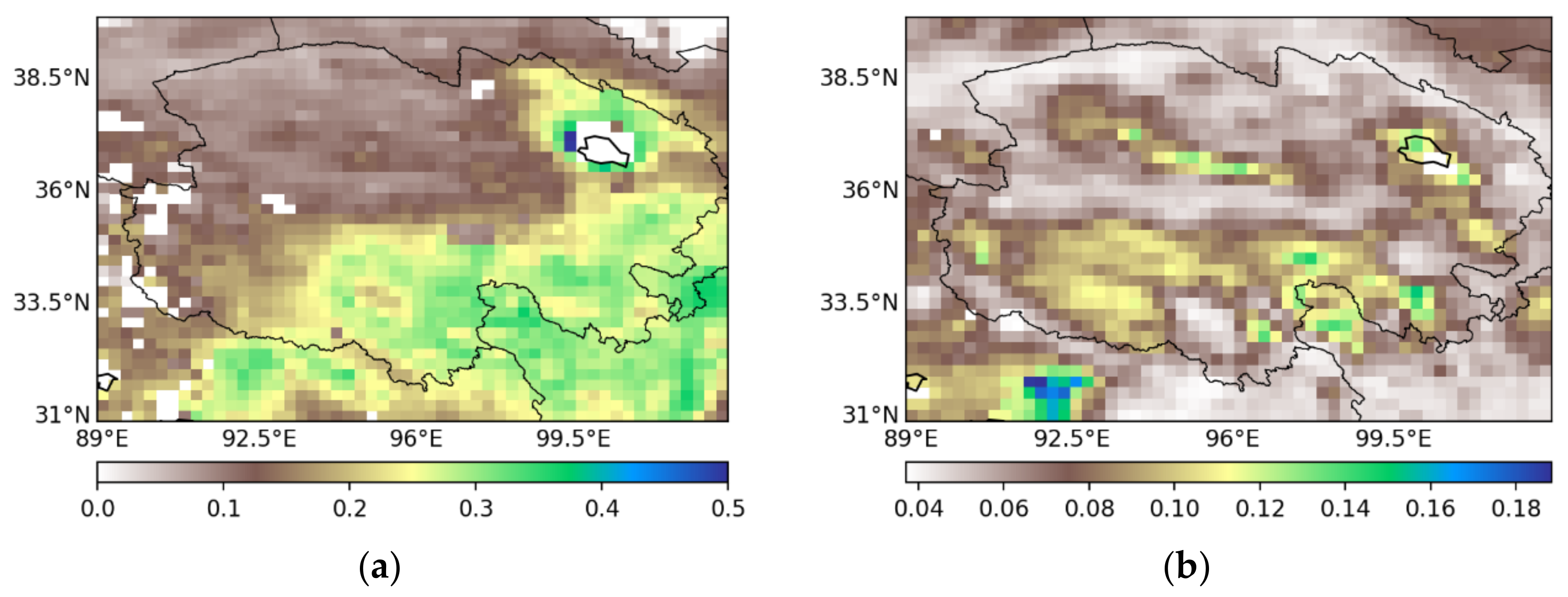
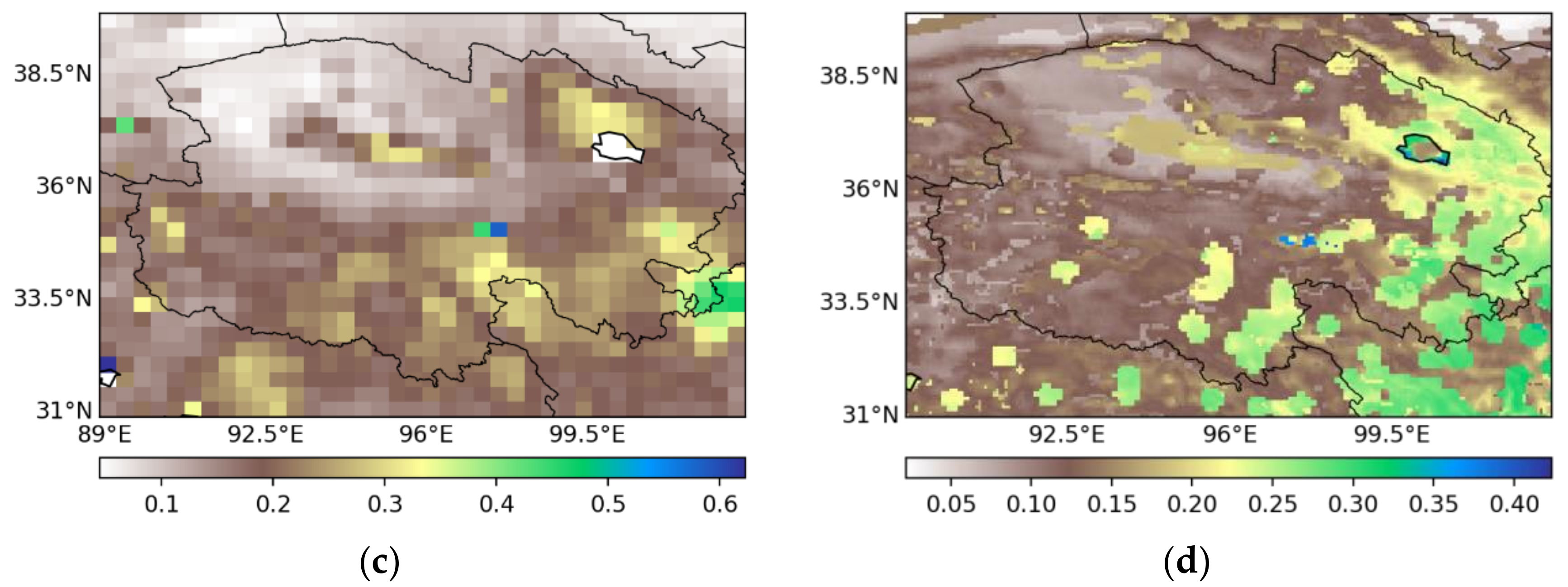
This study relies mainly on the passive microwave soil-moisture datasets SMAP, FY3C, and AMSR2 and the active microwave soil-moisture dataset of ASCAT as input microwave data. The datasets FY3C (10.65, 18.7, 23.8, 36.8, 89 GHz) and AMSR2 (6.925, 7.3, 10.65, 18.7, 23.8, 36.5, 89 GHz) have multiple frequencies, whereas SMAP (1.41 GHz) and ASCAT (5.3 GHz) have fixed frequencies; see Table 1 for details. In general, the L, C, and X bands are sensitive to SM, whereas other bands in other frequency ranges are not sensitive to SM. Therefore, this study uses the brightness temperature from the 1.41 GHz channel from SMAP, from the 6.9, 7.3, and 10.65 GHz channels of AMSR2, and from the 10.65 GHz channel of FY3C. Specifically, the SMAP radiometer uses a 24 MHz bandwidth centered at 1.41 GHz. The AMSR2 radiometer uses 0.35, 0.35, 0.10 GHz bandwidths centered at 6.9, 7.3, and 10.65 GHz, respectively. The FY3C radiometer uses a 180% ± 10% MHz bandwidth centered at 10.65 GHz. In addition, we use the backscatter coefficient (σ40) from the 5.3 GHz channel of the ASCAT active microwave data as the input variables for the NN. The specific spatial distribution of soil moisture is shown in Figure 1.
2.1.2. Data from Land Surface Model
As target data, we use the CLDAS soil volumetric water content analysis product, which is published by China Meteorological Data Service Centre. Comparing the quality-controlled SM observation data from automated monitoring stations in China with the CLDAS-V2.0 soil volumetric water content data shows that the CLDAS soil volumetric water content product fits the actual ground observation data [24], with a national regional average correlation coefficient of 0.89, a root mean square error (RMSE) of 0.02 m3/m3, and a deviation of 0.01 m3/m3. Therefore, CLDAS SM products are considered of higher quality than similar international products (such as the GLDAS and NLDAS products), and they also offer better spatial and temporal resolution. In addition, we use the SM data from the SM ground model GEOS-5 as the input product for triple collocation (TC). The GEOS-5 model provides hourly products, and this study uses the time of 05:30 for the surface SM dataset to represent the SM between 0 and 7 cm within the surface layer [25].
2.1.3. MODIS Data and Terrain Data
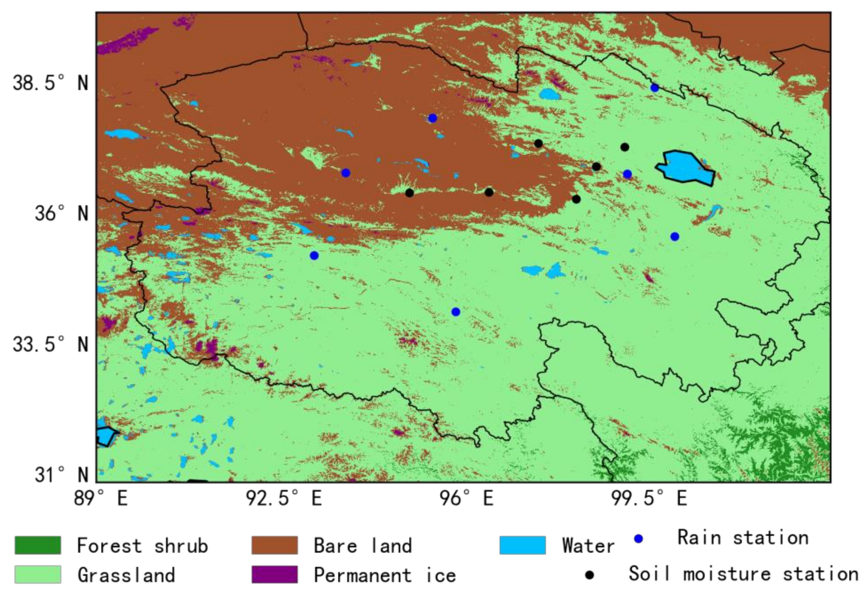
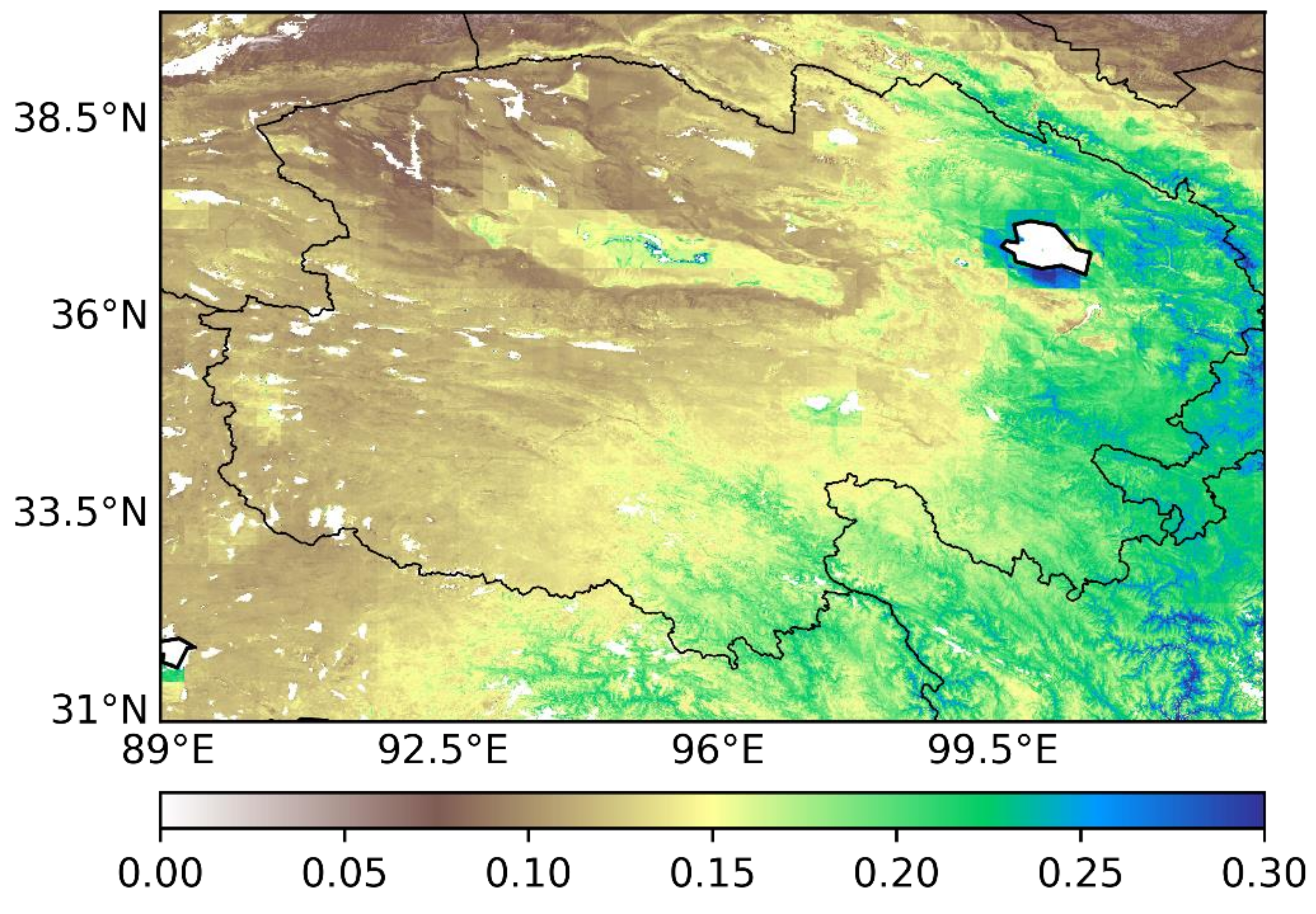
The auxiliary input data included land surface temperature (LST) and vegetation index (VI), and the VI data further included the enhanced VI (EVI) and the NDVI [26]. The daily LST data were provided by the MODIS-Terra LST product (MOD11A1) with a spatial resolution of 1 km. The EVI and NDVI data were provided by the MODIS-Terra VI products (MOD13A2) and have a temporal resolution of 16 days and a spatial resolution of 1 km. This study also uses data from the MODIS-Terra surface reflectance product (MOD09A1), with a temporal resolution of 8 days and a spatial resolution of 500 m. The annual land cover data (MCD12Q1) were also used here. The specific spatial distribution of vegetation cover is shown in Figure 2. In addition, we use the results of the SRTM 90-m digital elevation model (DEM) data and the calculated slope data (SLOPE) based on the DEM data for the study area. Table 2 summarizes the datasets used. The above data were obtained from the land processes distributed active archive center (https://lpdaac.usgs.gov/, accessed on 29 March 2021).
2.1.4. In Situ Observations
The measured data used in this paper are mainly divided into SM data and precipitation data from stations in Qinghai area. SM data are obtained from a soil depth of 10 cm and in time intervals of hours from six automated SM stations (Delingha, Dulan, Golmud, Nomuhong, Tianjun, and Wulan). The time interval for precipitation data is one day, and the areas contain the seven stations Yeniugou, Xiaozaohuo, Dachaidan, Chaka, Wudaoliang, Xinghai, Qumarai.
2.1.5. Data Preprocessing
Due to snow and ice coverage in winter, active and passive microwave data were not available from December to March in the study area because snow cover and frozen soil typically cover the land surface, which might introduce large biases in satellite-retrieved products such as SM [27]. Therefore, this study uses the satellite data and ground station data for Qinghai Province (31°–40° N, 89°–103° E) from 1 April 2017 to 30 November 2017 and from 1 April 2018 to 30 November 2018. To apply satellite observation data and SM data in the NN model, all data were resampled to a grid of 0.25° × 0.3125°. SMAP and AMSR2 data were treated by using bilinear interpolation, ASCAT and FY3C data by the inverse distance weighted method, and CLDAS, MODIS, and terrain data by simple average aggregation. Since the passive microwave datasets (SMAP, AMSR2, and FY3C) include both ascending and descending orbits, we processed the data from these orbits separately. In addition, the brightness temperature data of the passive microwave data could be divided into vertical and horizontal polarization channels, based on which the microwave polarization difference index (MPDI) is calculated as [28]
where Tbv and Tbh are the brightness temperature of the vertical and horizontal polarizations, respectively. Based on the assumption that the microwave channel is not subject to strong atmospheric attenuation, the MPDI is designed to eliminate the influence of surface temperature on microwave signals. In addition, it is a normalized polarization difference, which can serve as an indicator of SM status as a function of incident angle. In addition, the MPDI is sensitive to the dielectric properties of soil, and even more so to the surface roughness. Therefore, the MPDI is high for flat surfaces but relatively low for rough surfaces, such as areas with vegetation cover. In the preprocessing of the ASCAT data, the σ40 time series of each grid was renormalized to the range of [0 1], which means that the highest (lowest) backscatter value measured in this study is assigned the value 1 (0). The backscatter time index obtained from this preprocessed ASCAT data is abbreviated “BTI” [29]. This processing method emphasizes the time mode of the ASCAT signal and has been shown to reduce the retrieval time. However, since the processing is performed on the grid, it might reduce the spatial information provided by the radar.
MPDI = (Tbv − Tbh)/(Tbv + Tbh),
2.2. Method
2.2.1. Triple Collocation Method
The traditional error estimation method typically compares retrieved SM data with actual observation data obtained from ground stations. However, such comparisons are usually limited in number and location of instrument verification points, which makes it difficult to ensure robust datasets. In addition, the spatial mismatch between the ground data and the remote-sensing satellite data, as well as the heterogeneity of the ground surface, lead to representative errors and scale-conversion errors. Therefore, we used TC analysis [30,31,32] to estimate SM error. Compared with the traditional method to estimate SM error, it (1) does not require a high-quality reference dataset, which means that it can verify the three different SM data in the study area without ground measurement data. (2) Triple collocation simultaneously obtains the error variances of the three different SM data and (3) avoids the representative error caused by the spatial mismatch between the ground measurement data and the remote-sensing satellite data in the traditional estimation method. (4) Finally, the improved extended TC method [33] detects correlations between the retrieved SM data and the actual surface layer SM data. The error variance is expressed by [33]
where is the variance of X, and is the covariance of X and Y. The correlation coefficient is [33]
where is the correlation between X and the unknown true SM state.
In this study, the SMs retrieved by the NN method, collected from satellite data, and obtained from the ground model GEOS-5 are triple-matched in the form [NN data, satellite data, reanalysis data] to estimate the error variance and correlation coefficient of the TC. The SM obtained from the NN method is evaluated based on these results.
2.2.2. Evaluation Index
This study uses spatial correlation, temporal correlation, root mean square error, and mean absolute error to quantitatively analyze the aspects that differentiate SM retrieved by the NN and SM obtained from a model, as well as aspects that differentiate SM retrieved by the NN and SM collected from ground stations.
- (1)
- Spatial correlation: ρspatial
Spatial correlation serves to evaluate the accuracy with which the spatial model retrieves SM. It is obtained by calculating the Pearson correlation coefficient between the retrieved SM, which produces a daily correlation value between the whole area and the simulated SM map. For a better comparison, the average spatial correlation is calculated as the average of all daily spatial correlations with a significance greater than 95%.
- (2)
- Temporal correlation: ρtemporal
Temporal correlation is used to evaluate how well the retrieved SM matches the temporal variations in the SM. It is a location-related metric calculated at the pixel level. The Pearson correlation between the retrieved time series and the modeled SM is calculated for each pixel, which gives a correlation map. The mean temporal correlation is the mean value of all the pixels in the temporal correlation map.
- (3)
- Root mean square error: RMSE
The RMSE is calculated based on the unit error and the deviation from a reference of the unit error. Therefore, it provides a comprehensive assessment of recalculation, including the accuracy and precision of data retrieval. The RMSE is calculated at the pixel level by using the original SM time series, and a map of the RMSE is obtained for each retrieval. The mean RMSE is the mean value of all the pixels in the RMSE map.
- (4)
- Mean absolute error: MAE
The MAE is the absolute error between the retrieved SM and the simulated SM. It is calculated at the pixel level, and each search generates a map. The MAE correlation is the mean value of all the pixels in the MAE map.2.2.3. Downscaling scheme based on neural network.
A NN [34,35,36] is essentially a system to do nonlinear mathematical calculations and can represent any complex nonlinear process. The multivariable nature and nonlinear ability of NN fully exploit the synergy between different data. The NN used in this study has three parts: (1) an input layer, which receives the satellite observation data and auxiliary variable inputs; (2) a hidden layer; and (3) an output layer, which provides the SM. This structure suffices to fit any continuous function.
The NN was trained with satellite observation data as input data and the corresponding ground model data as target data. The training dataset must represent the entire range of expected scenarios, which means that it must include all climate regimes and seasons. If the training data are well selected, the NN’s performance when applied to the training data should differ little from its performance when applied to the entire dataset. Similarly, a NN should perform in the same way when applied to two sufficiently representative but completely different target datasets, meaning that any potential local or regional bias in the target data is corrected. These characteristics can be traced to the fact that the estimated spatial-temporal structure of the NN is determined by satellite observations instead of by target data [37]. In addition, the NN correlates the satellite observations with the most common SM among the input values in the target data, regardless of the location or acquisition time of the data [29].
The NN constructed in this study uses the Levenberg-Marquardt (LM) [38,39] training algorithm and applies error backpropagation [40] to update the weights. Since the LM algorithm stops when it finds a local minimum, the error surface is not fully explored. Therefore, in this study, the NN training was repeated four times, each time using random initial NN weights to ensure different starting points on the error surface; the optimal NN was selected for retrieving SM products.
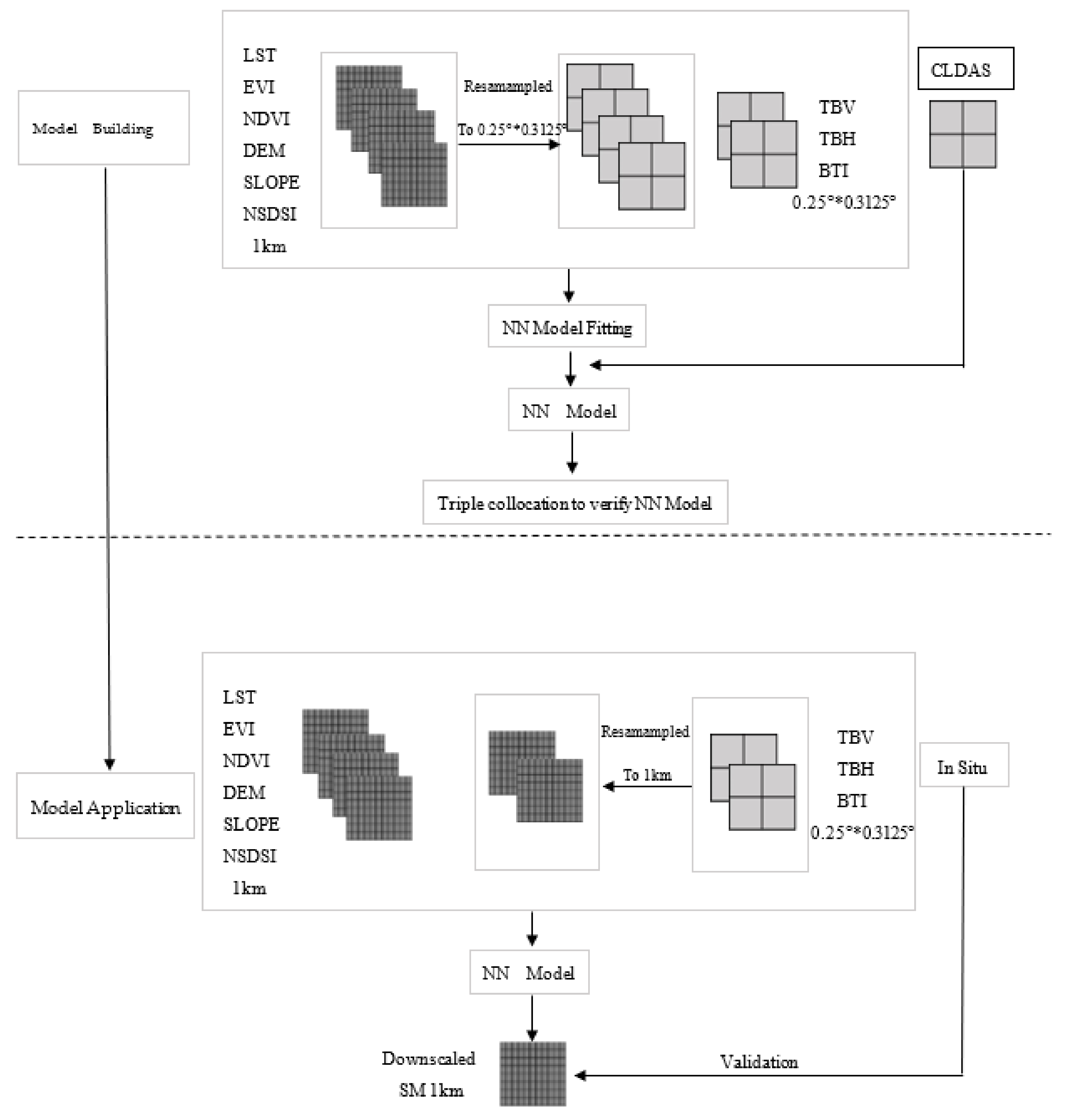
The key step in downscaling SM in this study is to build a statistical relationship using low spatial-resolution data, and then input high-spatial-resolution data into the statistical relationships to obtain the downscaled SM. [26,41,42] The spatial scale of different data is unified and scaled by different resampling methods, as shown in Section 2.1.5. In particular, the low-spatial-resolution microwave data are resampled to 1 km spatial resolution by replication expansion, without changing the specific values, to make them consistent with the spatial resolution of MODIS and other auxiliary data. Figure 3 shows a flow chart of this process, which is described as follows:
- Aggregate auxiliary data (NDVI, EVI, LST, NSDSI, DEM, and SLOPE) into a grid with a resolution of 0.25° × 0.3125°, which is consistent with the spatial resolution of the resampling microwave data (Tbh, Tbv, σ40, and BTI). Specific bands of microwave data are available in Section 2.1.1. The relationship between these different input variables and the ground model CLDAS SM was established through the NN, and the quality of the NN SM was evaluated by comparing it with the CLDAS SM.
- Evaluate the SM dataset obtained from the NN model by using the TC method.
- Input the 1 km medium-resolution data from 2017 to 2018 into the verified NN model to obtain 1-km-resolution SM data.
- Use the data collected from the ground station to verify the downscaled NN SM data.
3. Results and Discussion
3.1. Selection Microwave Band
By studying the quality of data retrieved from various satellites and in different bands, we identified the SM data from different sensors. This exercise was done using the CLDAS SM dataset as reference data. Although the NN model was trained on a small subset of the available dataset, the entire dataset was used for retrieval and evaluation. Table 3 summarizes the average quality index of the SM calculated by comparing a single microwave input dataset with the target SM dataset (CLDAS). Table 4 summarizes the average quality index of the SM calculated by comparing a combination microwave input dataset with the target SM dataset (CLDAS). Below, we discuss in detail the results of using different satellites and different bands.
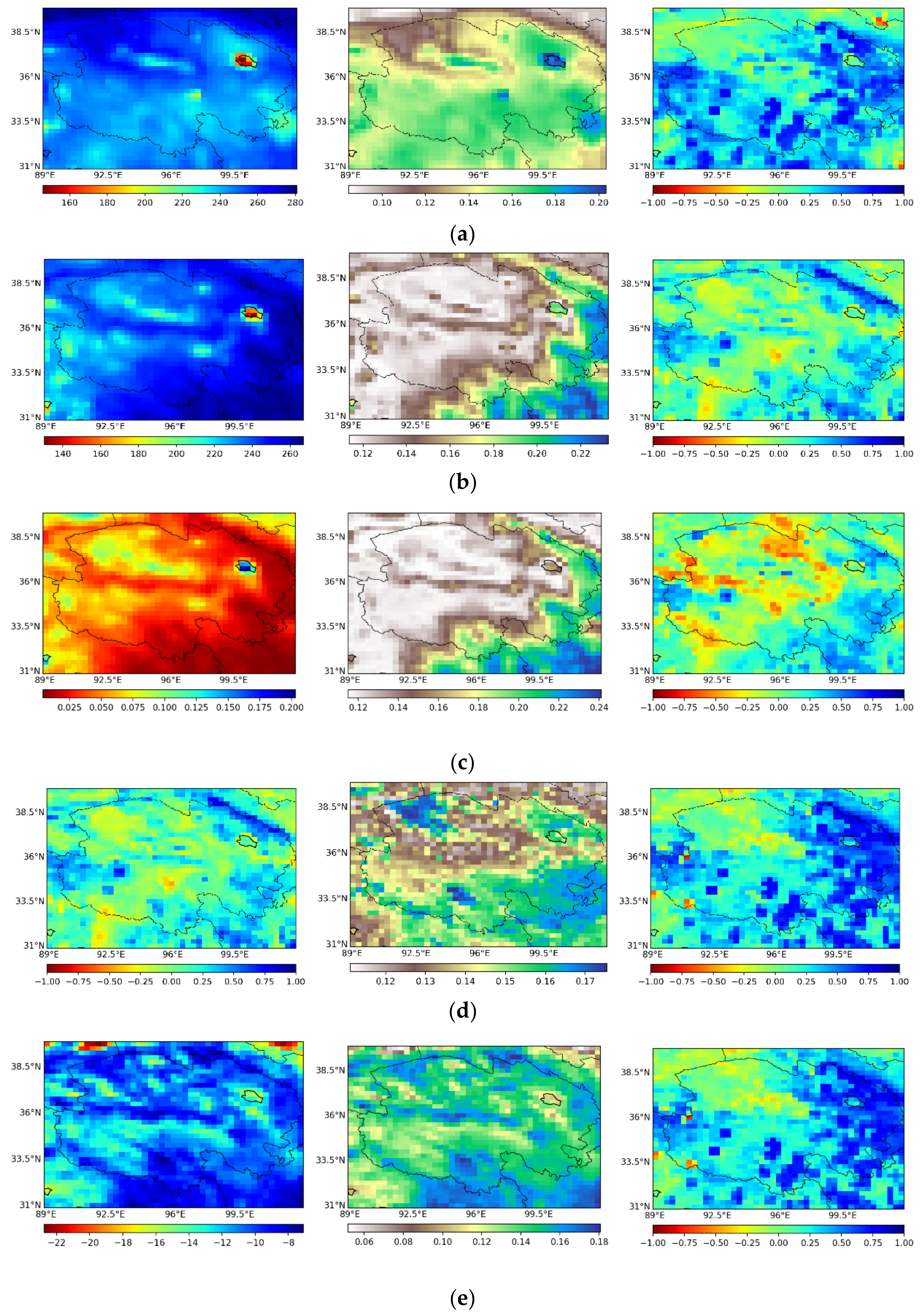
As shown in Table 3, in the 1.41 GHz (SMAP) band, Tbv has a higher spatial sensitivity to SM than Tbh, and the quality of Tbv in the ascending orbit exceeds that of Tbv in the descending orbit, with the average spatial correlation increased by 0.014 and the average temporal correlation increased by 0.087, and RMSE and MAE decreased by 0.001 and 0.002, respectively. In the 6.9, 7.3, and 10.7 GHz bands, Tbh is more sensitive to SM than is Tbv. In addition, the MPDI obtained from preprocessing in these bands also has greater spatial sensitivity to SM. Based on the AMSR2 microwave data, the 10.7 GHz band produces greater spatial and temporal correlation and lower RMSE and MAE in Qinghai Province compared with the 6.9 and 7.3 GHz bands and FY3C’s 10.7 GHz band, which indicate a higher sensitivity to SM. In addition, the experiments show that Tbh and MPDI are highly similar in terms of spatial distribution in the 6.9, 7.3, and 10.7 GHz bands but differ significantly from Tbv in the 1.41 GHz band, which leads to the assumption that complementary relationships exist between them. The processed BTI data were also more sensitive to soil moisture than the original σ40 data, with an increase of 0.01 in the average spatial correlation and an increase of 0.002 in the average temporal correlation, whereas the RMSE and MAE decreased by 0.002 and 0.001, respectively. Finally, the best microwave band combination in Qinghai province was selected by joint retrieval of Tbv in the ascending orbit of 1.41Ghz (SMAP) band, Tbh and MPDI in the descending orbit of 10.7Ghz (AMSR2) band, and BTI, σ40 data of ASCAT. Figure 4 shows the raw images of these five single bands, a map of daily average SM as obtained by the NN, and a map of the temporal correlation between the NN SM and the CLDAS SM, respectively.
Figure 4 shows the SM monitoring capability of different wavebands in Qinghai Province. The first row of Figure 4 shows that the original Tbv data at 1.41 GHz indicate higher temperatures in bare land and forest areas than in grassland areas, and both bare land and forest areas have lower daily average SM, which means that more information is needed to distinguish forest areas from bare lands when retrieving SM. Meanwhile, lake areas, such as the Qinghai Lake area in the northeast, are coolest. The temporal correlation map indicates a weak negative correlation in hotter areas (higher Tbv), such as the bare lands in the northwest (Qaidam Basin) and the bare lands in the northeast corner, and a strong positive correlation in cooler areas. The original Tbh maps in the second row reveal a high sensitivity to vegetation; combining these with the maps of average daily SM shows that higher vegetation coverage and higher temperature results in greater SM. However, the poor distinction between the bare lands in the northwest and the mixture of bare lands and grassland in the southwest indicates that more information is needed to distinguish between these two areas. The observation of the MPDI image in the third row shows a high similarity in spatial distribution with the TBH in the second row. The BTI maps in the fourth row show higher BTIs in the grassland in the southeast and in the hinterland of the Qaidam Basin in the northwest, which reflects greater SM in the SM map, and the mixture of bare lands and grassland around the Qaidam Basin has a lower BTI, which reflect a lower SM. Therefore, the correlation map shows a negative correlation of BTI in the northwest corner of Qaidam Basin and a strong positive correlation for the mixture of bare lands and grassland in the southwest and the mixture of bare lands and grassland in the northeast. The observation of the σ40 image in the fifth row shows that its spatial distribution is highly similar to that of the NN SM and CLDAS SM time correlation map of BTI in the fourth row. However, the differentiation between different areas of vegetation cover is worse in the SM map.
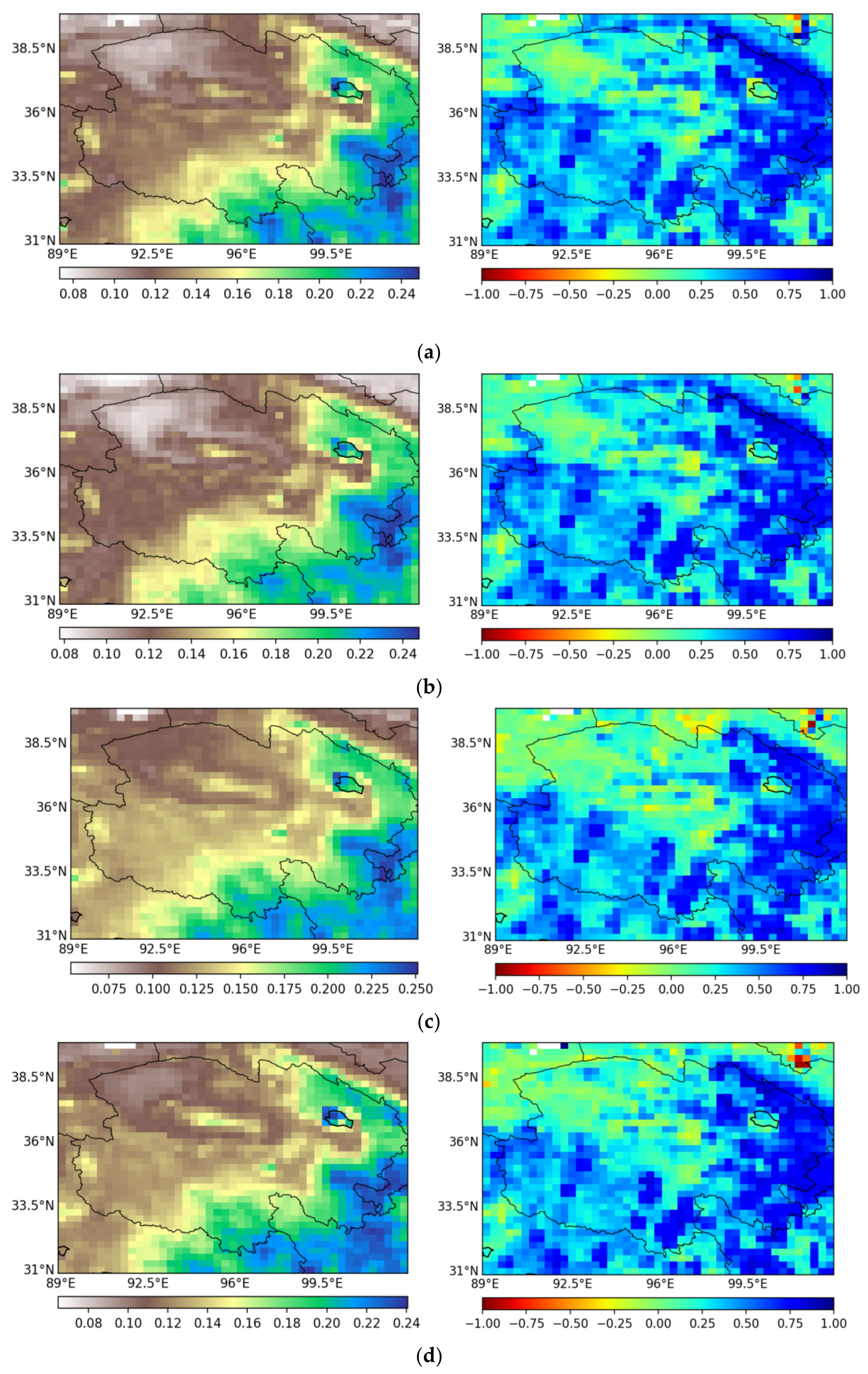
Figure 5 shows that the spatial distributions of SM obtained by NN retrieval of the four different combinations of data are highly similar to each other, and the overall SM increases from northwest to southeast, which clearly distinguishes bare soil areas, bare soil and grassland mixed areas, grassland areas, and forest areas, making up for the lack of detection capability of the single microwave band in Figure 4. Figure 5b,d with BTI data added at the same time do a better job distinguishing bare soil areas compared with Figure 5a,c with σ40 added [i.e., bare soil areas in Figure 5b,d have lower SM values and are better distinguished compared with grassland areas in the same image]. The NN SM and CLDAS SM time-correlation maps show that all four images are poorly correlated with CLDAS data in the northwest bare soil region and in the southeast corner of the mixed forest-steppe region but achieve better correlation in all other regions. Figure 5a,b show greater positive correlation in the northeast region than do Figure 5c,d, which confirms that the 10.7 Ghz (AMSR2) band descending-orbit TBH is more capable of detecting SM information in Qinghai province than is the 10.7Ghz (AMSR2) band descending-orbit MPDI.
The results in Table 4 show that the combined SMAP_TBV_A and AMSR2_TBH_D produce higher-quality SM data than the combination of SMAP_TBV_A and AMSR2_MPDI_D. Taking the CLDAS soil moisture data as a benchmark, for SMAP_TBV_A and AMSR2_TBH_D the combination spatial correlation and temporal correlation reach 0.621 and 0.393, respectively, for SMAP_TBV_A and AMSR2_MPDI_D the spatial correlation and temporal correlation reach 0.600 and 0.354, respectively. Meanwhile, given the high similarity between Tbh and MPDI (see Figure 4), AMSR2_TBH_D is used as a final input variable. Furthermore, the addition of σ40 and BTI to the above NN reduces the RMSE and MAE. Compared with the original σ40 data, BTI data obtained after preprocessing translate into a greater temporal correlation between the SM obtained by the NN model and CLDAS data. And based on experience, active and passive microwaves have different sensitivities to SM, vegetation, and surface roughness. The 5.3 GHz observation frequency of ASCAT also differs significantly from that of SMAP (1.41 GHz) and AMSR2 (10.7 GHz). Therefore, the ASCAT dataset is considered as a potentially useful dataset that could compensate for the combination of passive microwave data in the NN. BTI is used as a final input variable.
Finally, the input variables are ascending Tbv in the 1.41 GHz (SMAP) band, descending Tbh in the 10.7 GHz (AMSR2) band, and BTI data from ASCAT.
3.2. Selection of Auxiliary Data
This section discusses the results of a collaborative analysis of microwave data and auxiliary input data for SM retrieval. The purpose is to determine the content and type of information that can be extracted from microwave data and auxiliary observation data and determine how to combine these data to provide maximal information for SM retrieval. Experimental trials were conducted to add and combine various auxiliary input data based on microwave data and to retrieve SM from different combinations of datasets using the NN model. These results are compared with the CLDAS data to determine the optimal combination (see detailed results in Table 5). In addition, for completeness, the SM products retrieved from all available data are compared among themselves.
The brightness temperature and backscattering coefficient obtained by active and passive microwave data are all affected by the opacity of vegetation cover, which reduces the radiation from the soil surface. Therefore, information about the vegetation strongly affects SM retrieval. Table 5 also shows that adding the VI data to the microwave data improves spatial and temporal correlations and reduces MAE and RMSE. Compared with EVI, NDVI improves the spatial correlation to 0.623. Given the high correlation between NDVI and EVI, NDVI is used as a final input variable.
Terrain data such as DEM and SLOPE also play an important role in the retrieval of SM by physical models. The complex mountainous terrain reduces the quality of the microwave data retrieved. In addition, precipitation is mainly concentrated at higher altitudes in many areas of Qinghai Province, leading to relatively lush vegetation cover, which strongly affects the SM. As a result, DEM and SLOPE are also used as final input variables. Table 5 shows that adding DEM to the NN model improves the spatial correlation to 0.634 and the temporal correlation to 0.412. When NDVI, DEM, and SLOPE are all added to the NN model, the spatial correlation reaches 0.676, and the temporal correlation reaches 0.450. The surface temperature information strongly affects the soil surface emissivity, which directly affects the brightness temperature and the backscatter coefficient. Table 5 shows that when a single auxiliary input variable for the NN model, adding LST produces the greatest improvement of the temporal correlation, which attains 0.441.
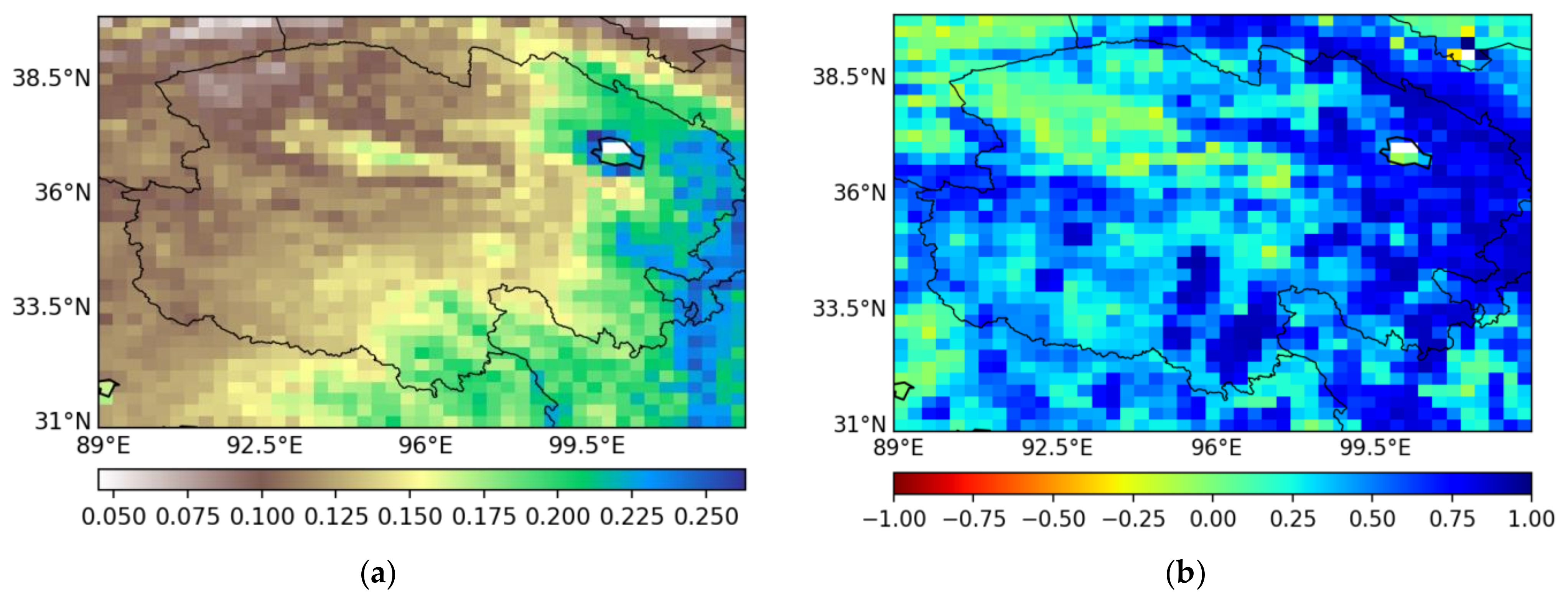
Compared with CLDAS data, the SM retrieved (see Table 5) from the combination of microwave data and auxiliary inputs NSDSI, NDVI, DEM, and SLOPE produces the highest spatial correlation of 0.684, whereas the temporal correlation is only 0.453. The SM retrieved from the combination of microwave data and auxiliary inputs LST, NDVI, DEM, and SLOPE produces the highest temporal correlation of 0.477, whereas the spatial correlation is only 0.663. The SM retrieved from the combination of microwave data and auxiliary inputs NSDSI, LST, NDVI, DEM, and SLOPE produces a spatial correlation of 0.669 and a temporal correlation of 0.475, which is the most balanced combination. Therefore, we use herein the microwave data and auxiliary inputs NDVI, DEM, SLOPE, LST, NSDSI, etc. as final input variables to obtain the daily average SM map of Qinghai Province, which is shown on the left side of Figure 6. On the right side of Figure 4 is shown the correlation map between SM data retrieved from the NN and CLDAS SM data.
Figure 6 shows that the overall SM in the entire study area increases from northwest to southeast. Also, the high positive correlation in the grassland areas and poor correlations in the Qaidam Basin (northwest corner) and the mixture of forest and grassland (southeast corner) show that the above input variables do not allow us to retrieve SM from bare lands and forest areas but do allow us to retrieve SM from grassland areas.
3.3. Triple Collocation Method to Verify Soil Moisture as Determined by Neural Network
To estimate how accurately the NN model determines the SM on a large scale, we apply TC to analyze the SM from the NN. TC estimates the distribution of spatial error for each dataset by locally solving the linear relationships between the three SM datasets. One of the assumptions is that the errors in all three datasets are independent, so the FY3C SM data, which were not used to train the NN model, are combined with the GEOS-5 ground-model SM data and the SM data used to train the NN model in the form of [NN SM, FY3C SM, GEOS-5 SM] for TC. Furthermore, to ensure the accuracy of the TC results, the areas with a correlation coefficient between the three different datasets less than 0.2 are masked and are not involved in the final TC calculation. Finally, the error variance and correlation coefficient are estimated between the NN data and the actual SM data.
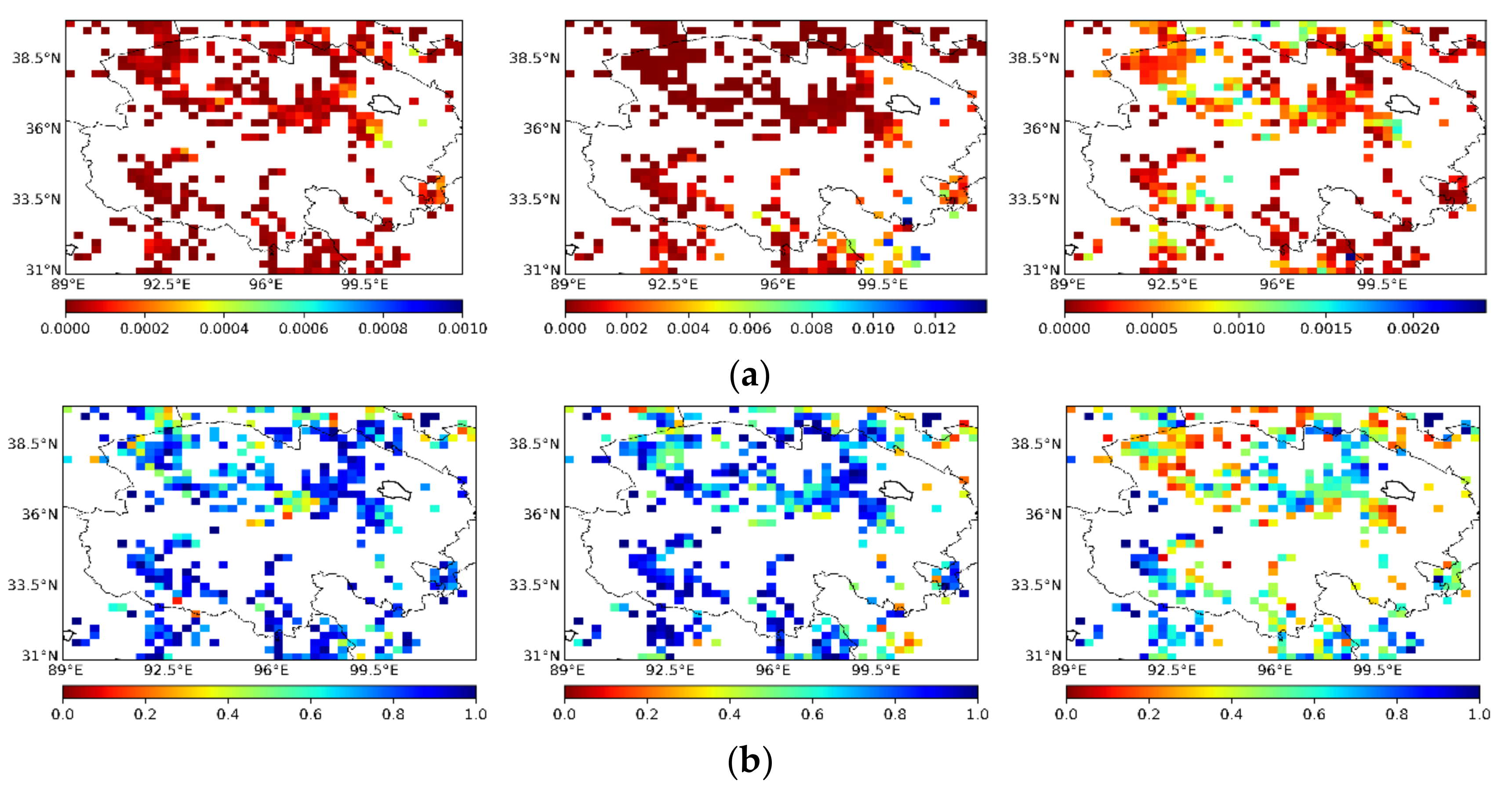
The spatial distribution shown in Figure 7 of the variance in TC error indicates that the variance in error between the SM retrieved from NN and FY3C and the actual SM is lowest in the Qaidam Basin in the northwest, whereas the variance in the error between the SM retrieved from GEOS-5 and the actual SM in the Qaidam Basin area is significantly greater. Combining these results with the maps of the spatial distribution of TC correlation coefficients shows that the spatial distribution of the correlation coefficient between the SM retrieved from NN and FY3C and the actual SM correlates to the error variance, meaning that the areas with greater error variance correlate more to the actual SM data.
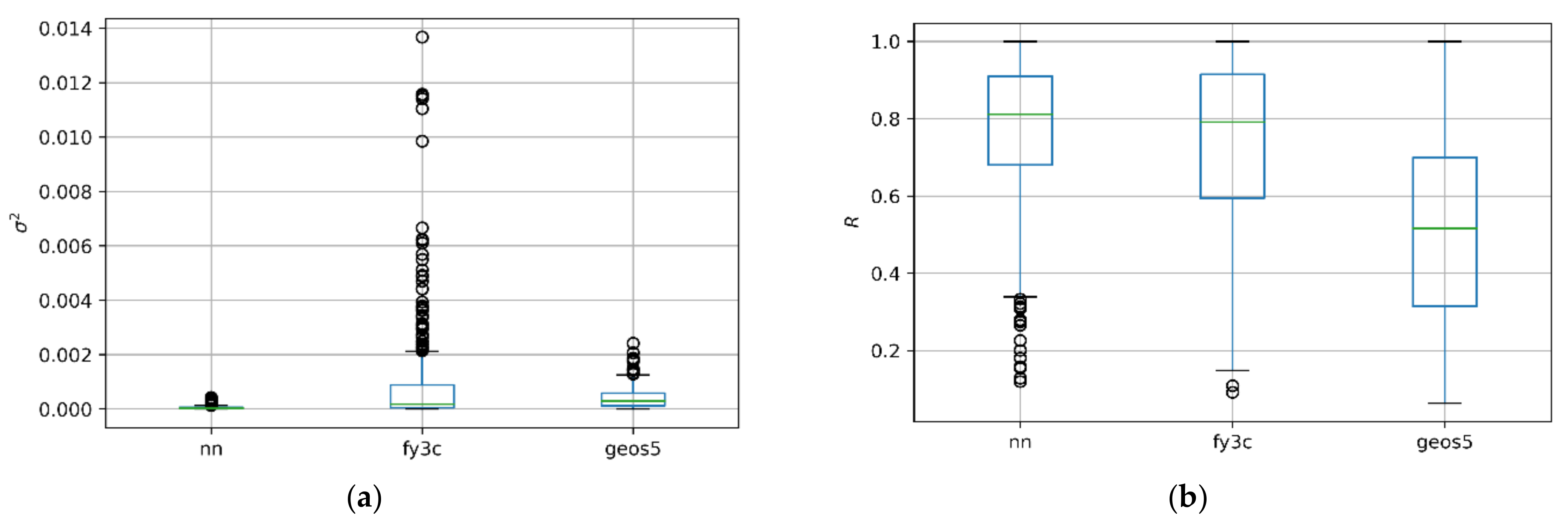
Figure 8 show that the error variance between NN SM and the actual SM is much less than the error variance between (i) FY3C SM and GEOS-5 SM and (ii) the actual SM, with a median error variance of 0.0003 (NN) < 0.00017 (FY3C) < 0.00030 (GEOS-5). The correlation coefficient between (i) NN SM and FY3C SM and (ii) the actual SM is much greater than that for GEOS-5 SM, with a median correlation coefficient of 0.811 (NN) > 0.792 (FY3C) > 0.516 (GEOS-5). Among these three datasets, NN and FY3C have similar median correlation coefficients, but NN has Q1 = 0.681 and a lower-limit outlier of 0.338, which are much greater than for FY3C (Q1 = 0.594 and lower-limit outlier of 0.115). Therefore, after comprehensive analysis and comparison, the SM data retrieved by the NN model is of better quality for Qinghai Province.
3.4. Verification of Downscaled Soil Moisture from Neural Network
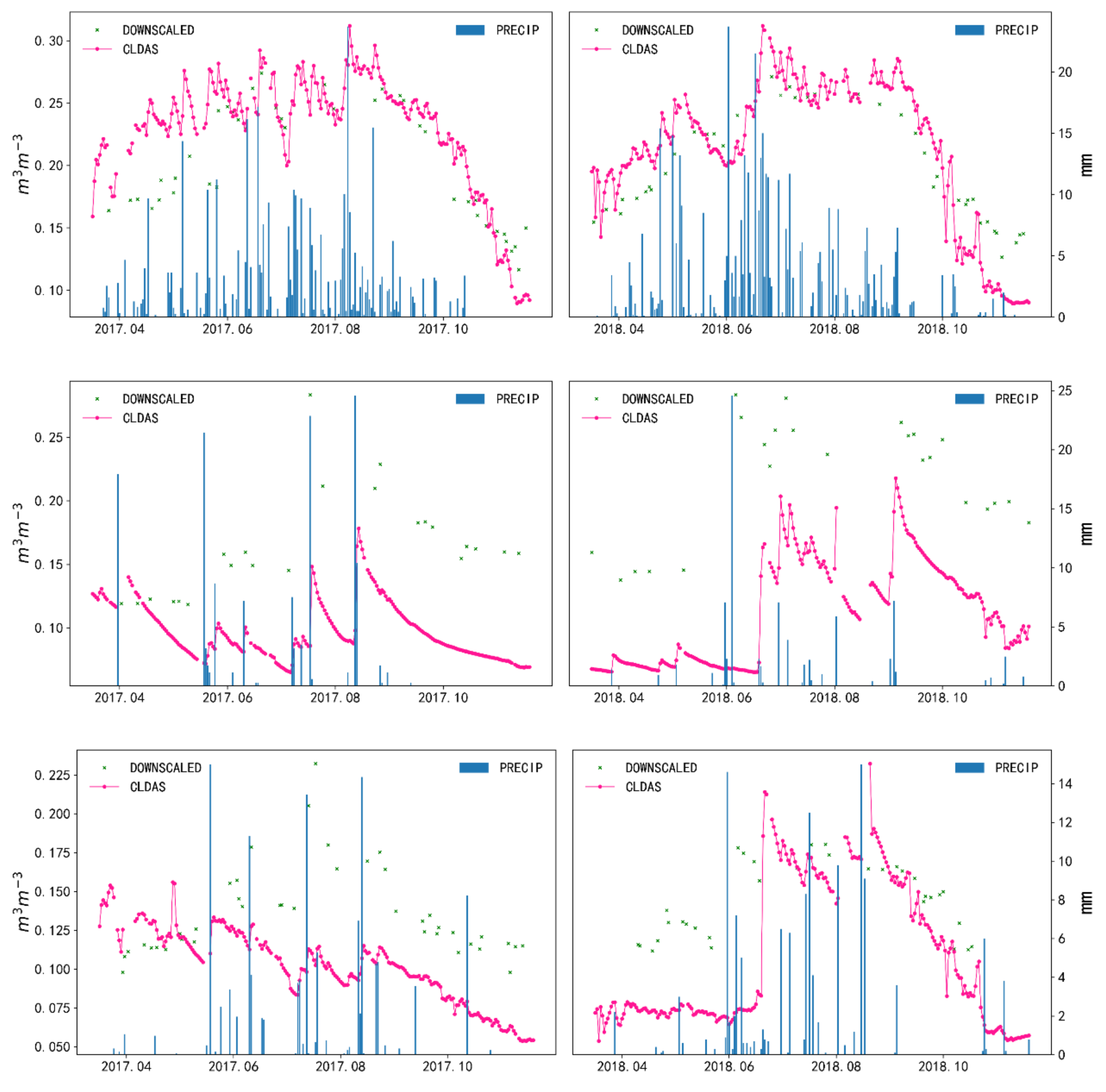
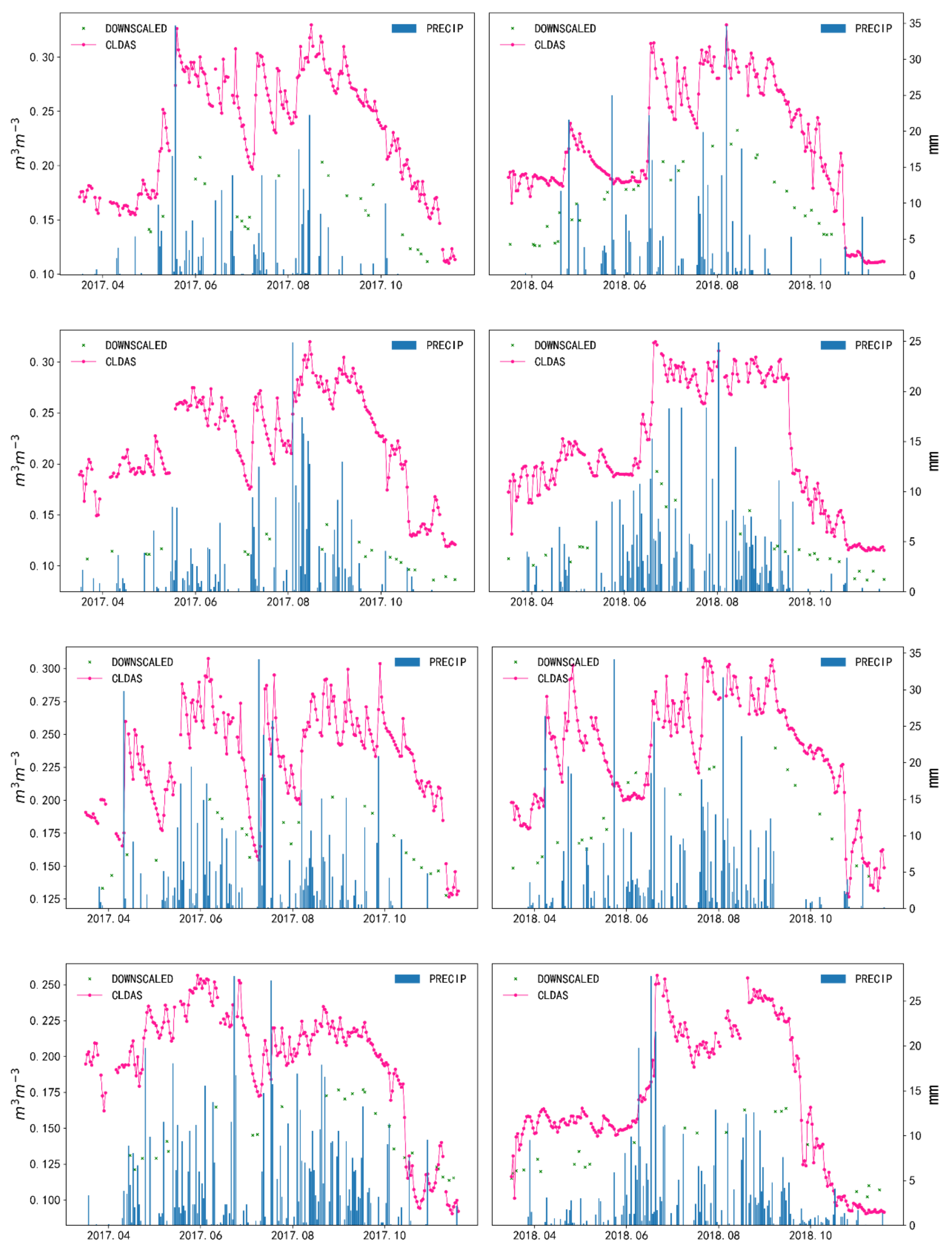
In this study, the downscaled SM dataset for Qinghai Province and the map of the daily average SM (Figure 9) were obtained by inputting MODIS data with high spatial resolution and resampled microwave data into the NN model verified by the TC. To verify the adaptability of the downscaled SM data for Qinghai Province, we apply a correlation analysis where we compare the downscaled 1 km SM data, original SMAP SM data, original AMSR2 SM data, and CLDAS SM data with the SM data collected from six ground stations in Qinghai Province. In terms of data selection, for each time series, we use data from all available at ground stations and from CLDAS, SMAP, AMSR2, and NN. In addition, each time series extends over at least 30 days to obtain good statistics. Furthermore, to determine whether the downscaled SM data capture the actual ground SM dynamics, we verify the variations over time of the downscaled SM by studying the time series of the seven ground precipitation stations (see Figure 10).
Table 6 shows that the correlation of the downscaled SM results of the NN model at the Dulan, Tianjun, and WuUlan sites exceeds 0.6, which is a larger average than CLDAS, SMAP, and AMSR2, thereby demonstrating that the NN model properly downscales the SM. Table 6 also reveals negative correlations with CLDAS SM at both the Golmud and Nuomuhong sites, whereas SMAP, AMSR2, and NN produce negative correlations at the Golmud site but positive correlations at the Nuomuhong site. This indicates that the temporal and spatial structures based on the NN model are driven by the satellite observations rather than by the target data. Figure 7 shows a map of the daily average SM in Qinghai Province after downscaling; these results provide much more SM information than do large-scale maps of SM.
Figure 10 shows that the downscaled SM strongly correlates with the precipitation data because the SM increases significantly after precipitation and decreases significantly during drought. Furthermore, the downscaled SM data from Xiaozaohuo, Chaka, Wudaoliang and other sites depart significantly from the absolute value of the CLDAS data, whereas both maintain good time consistency. The results demonstrate that downscaling the SM captures better the variations in precipitation over time, which indicates that the downscaled SM better reflects the actual variations in SM over time.
4. Conclusions
This paper presents a method to retrieve soil moisture (SM) by combining multi-instrument observation data. The method is based on a neural network (NN) to retrieve SM information from passive microwave sensors SMAP and AMSR2, active microwave sensors ASCAT, as well as MODIS data (LST, NSDSI, NDVI) and topographic data (DEM, SLOPE). The greatest advantage of this method is that it can give full play to the potential of the joint retrieval of SM by each microwave sensor and also make full use of the segmentation capability of high-spatial-resolution MODIS data and topographic data.
From the microwave band selection, the best retrieval effect was achieved by the combination of Tbv in the ascending orbit for the 1.41 GHz (SMAP) band, Tbh in the descending orbit for the 10.7 GHz (AMSR2) band, and BTI data of ASCAT through the neural network method. The final NN SM dataset is obtained by combining the auxiliary data LST, NDVI, NSDSI, DEM, and SLOPE with the above three bands of microwave data. The above two models were compared with the CLDAS model SM dataset, and the result shows that the spatial correlation increases from 0.597 to 0.669, the temporal correlation increases from 0.401 to 0.475, the root mean square error decreases from 0.051 to 0.046, and the mean absolute error decreases from 0.041 to 0.036. All indicators improve, which confirms that the use of the auxiliary data improves the performance of the NN model.
The low-resolution SM products obtained from the NN retrieval in the triple collocation are higher quality than the SM products from the FY3C satellite and the ground model GEOS5 in Qinghai Province (i.e., the NN low-resolution products have the highest median correlation of 0.811, the highest correlation Q1 value of 0.681, and the lowest error variance of 0.00003).
Based on the comparison with the ground stations data, the NN SM dataset obtained on the small scale is also of better quality than the CLDAS product, and the correlation with SM at three stations, namely, Dulan (0.768), Tianjun (0.620), and Wulan (0.616), exceeds 0.6, showing strong correlation. The correlation between CLDAS SM products is greater than 0.6 only in Dulan (0.759) and Wulan (0.670). In addition, comparing with the rainfall site data shows that downscaled NN SM data also better capture the dynamic changes of SM in the study area, producing higher SM values when there is more rainfall and a decrease in SM during the long dry season. Comparing the images before and after downscaling also shows that the SM after downscaling can provide more detailed SM information. We also discuss some shortcomings in the downscaling process. The downscaled SM is susceptible to interference from clouds and rain, leading to a significant quantity of missing data, so future work will focus on data completion.
The results of this study confirm that the NN method can be used to obtain SM with high spatial resolution and can be applied to the Qinghai Province area. The data used herein can be downloaded for free from the official websites of the National Aeronautics and Space Administration (NASA), the Japan Aerospace Exploration Agency (JAXA), the European Centre for Medium-Range Weather Forecasts (ECMWF), and the China Meteorological Information Sharing Platform (CIMISS) without regional restrictions and can be used to produce sTable 1 km SM data in the Qinghai Province area.
Author Contributions
A.L. designed and conduct the study. Z.Z. performed the data analysis and wrote the manuscript. H.Z. read and edited the manuscript. All authors reviewed and approved the manuscript. All authors have read and agreed to the published version of the manuscript.
Funding
This research was funded the National Natural Science Foundation of China (41671026), the Important Science & Technology Specific Projects of Qinghai Province (2019-SF-A4-1) and Scientific Research and Promotion Projects of the Second Phase Project of Ecological Protection and Construction of the Three Rivers Source in Qinghai Province (2018-S-3).
Institutional Review Board Statement
Not applicable.
Informed Consent Statement
Not applicable.
Data Availability Statement
The data used in this study were downloaded from the National Aeronautics and Space Administration (NASA), the Japan Aerospace Exploration Agency (JAXA), the European Centre for Medium-Range Weather Forecasts (ECMWF), and the China In-tegrated Meteorological Information Service System (CIMISS).
Acknowledgments
We are very grateful to the teams at NASA, JAXA, ECMWF, and CIMISS who have made their datasets available and ready to use.
Conflicts of Interest
The authors declare no conflict of interest.
References
- McColl, K.A.; Alemohammad, S.H.; Akbar, R.; Konings, A.G.; Yueh, S.; Entekhabi, D. The global distribution and dynamics of surface soil moisture. Nat. Geosci. 2017, 10, 100–104. [Google Scholar]
- Peng, J.; Loew, A.; Merlin, O.; Verhoest, N.E.C. A review of spatial downscaling of satellite remotely sensed soil moisture. Rev. Geophys. 2017, 55, 341–366. [Google Scholar]
- Keshavarz, M.R.; Vazifedoust, M.; Alizadeh, A. Drought monitoring using a Soil Wetness Deficit Index (SWDI) derived from MODIS satellite data. Agric. Water Manag. 2014, 132, 37–45. [Google Scholar]
- Rosenzweig, C.; Tubiello, F.N.; Goldberg, R.; Mills, E.; Bloomfield, J. Increased crop damage in the US from excess precipitation under climate change. Glob. Environ. Chang. 2002, 12, 197–202. [Google Scholar]
- Miller, G.R.; Baldocchi, D.D.; Law, B.E. Meyers An analysis of soil moisture dynamics using multi-year data from a network of micrometeorological observation sites. Adv. Water Resour. 2007, 30, 1065–1081. [Google Scholar]
- Mladenova, I.; Lakshmi, V.; Jackson, T.J.; Walker, J.P.; Merlin, O.; Jeu, R.A.M. De Validation of AMSR-E soil moisture using L-band airborne radiometer data from National Airborne Field Experiment 2006. Remote Sens. Environ. 2011, 115, 2096–2103. [Google Scholar]
- Zhang, P.; Yang, J.; Dong, C.; Lu, N.; Yang, Z.; Shi, J. General introduction on payloads, ground segment and data application of Fengyun 3A. Front. Earth Sci. China 2009, 3, 367–373. [Google Scholar]
- Zabolotskikh, E.V.; Mitnik, L.M.; Chapron, B. New approach for severe marine weather study using satellite passive microwave sensing. Geophys. Res. Lett. 2013, 40, 3347–3350. [Google Scholar]
- Kerr, Y.H.; Waldteufel, P.; Wigneron, J.P.; Delwart, S.; Cabot, F.; Boutin, J.; Escorihuela, M.J.; Font, J.; Reul, N.; Gruhier, C.; et al. The SMOS L: New tool for monitoring key elements ofthe global water cycle. Proc. IEEE 2010, 98, 666–687. [Google Scholar]
- Medeiros, J. Design and Development of the SMAP Microwave Radiometer Electronics. In Proceedings of the Specialist Meeting on Microwave Radiometry and Remote Sensing of the Environment, Pasadena, CA, USA, 24–27 March 2014. [Google Scholar]
- Figa-Saldaña, J.; Wilson, J.J.W.; Attema, E.; Gelsthorpe, R.; Drinkwater, M.R.; Stoffelen, A. The advanced scatterometer (ascat) on the meteorological operational (MetOp) platform: A follow on for european wind scatterometers. Can. J. Remote Sens. 2002, 28, 404–412. [Google Scholar]
- Njoku, E.G.; Wilson, W.J.; Yueh, S.H.; Dinardo, S.J.; Bolten, J. Observations of soil moisture using a passive and active low-frequency microwave airborne sensor during SGP99. Geosci. Remote Sens. IEEE Trans. 2002, 40, 2659–2673. [Google Scholar]
- Das, N.N.; Entekhabi, D.; Njoku, E.G. An algorithm for merging SMAP radiometer and radar data for high-resolution soil-moisture retrieval. IEEE Trans. Geosci. Remote Sens. 2011, 49, 1504–1512. [Google Scholar]
- Zhan, X.; Houser, P.R.; Walker, J.P.; Crow, W.T. A method for retrieving high-resolution surface soil moisture from hydros L-band radiometer and radar observations. IEEE Trans. Geosci. Remote Sens. 2006, 44, 1534–1544. [Google Scholar]
- Wilson, D.J.; Western, A.W.; Grayson, R.B. A terrain and data-based method for generating the spatial distribution of soil moisture. Adv. Water Resour. 2005, 28, 43–54. [Google Scholar]
- Srivastava, P.K.; Han, D.; Ramirez, M.R.; Islam, T. Machine Learning Techniques for Downscaling SMOS Satellite Soil Moisture Using MODIS Land Surface Temperature for Hydrological Application. Water Resour. Manag. 2013, 27, 3127–3144. [Google Scholar]
- Yang, K.; Zhu, L.; Chen, Y.; Zhao, L.; Qin, J.; Lu, H.; Tang, W.; Han, M.; Ding, B.; Fang, N. Land surface model calibration through microwave data assimilation for improving soil moisture simulations. J. Hydrol. 2016, 533, 266–276. [Google Scholar]
- Chen, W.; Shen, H.; Huang, C.; Li, X. Improving soil moisture estimation with a dual ensemble Kalman smoother by jointly assimilating AMSR-E brightness temperature and MODIS LST. Remote Sens. 2017, 9, 273. [Google Scholar]
- Chauhan, N.S.; Miller, S.; Ardanuy, P. Spaceborne soil moisture estimation at high resolution: A microwave-optical/IR synergistic approach. Int. J. Remote Sens. 2003, 24, 4599–4622. [Google Scholar]
- Liu, Z.; Zhou, P.; Zhang, F. Spatiotemporal characteristics of dryness/wetness conditions across Qinghaiprovince, Northwest China. Agric. For. Meteorol. 2013, 182–183, 101–108. [Google Scholar]
- Qi, Y.; Li, S.; Ran, Y.; Wang, H.; Wu, J.; Lian, X.; Luo, D. Mapping Frozen Ground in the Qilian Mountains in 2004–2019 Using Google Earth Engine Cloud Computing. Remote Sens. 2021, 13, 149. [Google Scholar]
- Liu, S.; Zhang, Y.; Cheng, F.; Hou, X.; Zhao, S. Response of Grassland Degradation to Drought at Different Time-Scales in Qinghai Province: Spatio-Temporal Characteristics, Correlation, and Implications. Remote Sens. 2017, 9, 1329. [Google Scholar]
- Cui, Y.; Long, D.; Hong, Y.; Zeng, C.; Zhou, J.; Han, Z.; Liu, R.; Wan, W. Validation and reconstruction of FY-3B/MWRI soil moisture using an artificial neural network based on reconstructed MODIS optical products over the Tibetan Plateau. J. Hydrol. 2016, 543, 242–254. [Google Scholar]
- Shi, C.; Xie, Z.; Qian, H.; Liang, M.; Yang, X. China land soil moisture EnKF data assimilation based on satellite remote sensing data. Sci. China Earth Sci. 2011, 54, 1430–1440. [Google Scholar]
- Lucchesi, R. File Specification for GEOS-5 FP; NASA Global Modeling and Assimilation Office (GMAO) Office Note No. 4 (Version 1.0); NASA: Washington, DC, USA, 2013. [Google Scholar]
- Hu, F.; Wei, Z.; Zhang, W.; Dorjee, D.; Meng, L. A spatial downscaling method for SMAP soil moisture through visible and shortwave-infrared remote sensing data. J. Hydrol. 2020, 590, 125360. [Google Scholar]
- Van der Vliet, M.; Van der Schalie, R.; Rodriguez-Fernandez, N.; Colliander, A.; de Jeu, R.; Preimesberger, W.; Scanlon, T.; Dorigo, W. Reconciling Flagging Strategies for Multi-Sensor Satellite Soil Moisture Climate Data Records. Remote Sens. 2020, 12, 3439. [Google Scholar]
- Ghulam, A.; Qin, Q.; Teyip, T.; Li, Z.-L. Modified perpendicular drought index (MPDI): A real-time drought monitoring method. ISPRS J. Photogramm. Remote Sens. 2007, 62, 150–164. [Google Scholar]
- Kolassa, J.; Gentine, P.; Prigent, C.; Aires, F. Soil moisture retrieval from AMSR-E and ASCAT microwave observation synergy. Part 1: Satellite data analysis. Remote Sens. Environ. 2016, 173, 1–14. [Google Scholar]
- Scipal, K.; Holmes, T.; De Jeu, R.; Naeimi, V.; Wagner, W. A possible solution for the problem of estimating the error structure of global soil moisture data sets. Geophys. Res. Lett. 2008, 35, 2–5. [Google Scholar]
- Gruber, A.; Su, C.-H.; Zwieback, S.; Crow, W.; Dorigo, W.; Wagner, W. Recent advances in (soil moisture) triple collocation analysis. Int. J. Appl. Earth Obs. Geoinf. 2016, 45, 200–211. [Google Scholar]
- Chen, F.; Crow, W.T.; Bindlish, R.; Colliander, A.; Burgin, M.S.; Asanuma, J.; Aida, K. Global-scale evaluation of SMAP, SMOS and ASCAT soil moisture products using triple collocation. Remote Sens. Environ. 2018, 214, 1–13. [Google Scholar]
- McColl, K.A.; Vogelzang, J.; Konings, A.G.; Entekhabi, D.; Piles, M.; Stoffelen, A. Extended triple collocation: Estimating errors and correlation coefficients with respect to an unknown target. Geophys. Res. Lett. 2014, 41, 6229–6236. [Google Scholar]
- Paloscia, S.; Pettinato, S.; Santi, E.; Notarnicola, C.; Pasolli, L.; Reppucci, A. Soil moisture mapping using Sentinel-1 images: Algorithm and preliminary validation. Remote Sens. Environ. 2013, 134, 234–248. [Google Scholar]
- Ge, L.; Hang, R.; Liu, Y.; Liu, Q. Comparing the performance of neural network and deep convolutional neural network in estimating soil moisture from satellite observations. Remote Sens. 2018, 10, 1327. [Google Scholar]
- Kolassa, J.; Reichle, R.H.; Liu, Q.; Alemohammad, S.H.; Gentine, P.; Aida, K.; Asanuma, J.; Bircher, S.; Caldwell, T.; Colliander, A.; et al. Estimating surface soil moisture from SMAP observations using a Neural Network technique. Remote Sens. Environ. 2018, 204, 43–59. [Google Scholar] [PubMed]
- Rodríguez-Fernández, N.J.; Aires, F.; Richaume, P.; Kerr, Y.H.; Prigent, C.; Kolassa, J.; Cabot, F.; Jiménez, C.; Mahmoodi, A.; Drusch, M. Soil moisture retrieval using neural networks: Application to SMOS. IEEE Trans. Geosci. Remote Sens. 2015, 53, 5991–6007. [Google Scholar]
- Levenberg, K. A Method for the Solution of Certain Nonlinear Problems in Least Squares. Q. Appl. Math. 1944, 2, 164–168. [Google Scholar]
- Marquardt, D.W. An Algorithm for Least-Squares Estimation of Nonlinear Parameters. J. Soc. Ind. Appl. Math. 1963, 11, 431–441. [Google Scholar]
- Rumelhart, D.E.; Chauvin, Y. Backpropagation: Theory, Architectures, and Applications; Psychology Press: Hove, UK, 1995. [Google Scholar]
- Piles, M.; Petropoulos, G.P.; Sánchez, N.; González-Zamora, Á.; Ireland, G. Towards improved spatio-temporal resolution soil moisture retrievals from the synergy of SMOS and MSG SEVIRI spaceborne observations. Remote Sens. Environ. 2016, 180, 403–417. [Google Scholar]
- Piles, M.; Camps, A.; Vall-Llossera, M.; Corbella, I.; Walker, J.P. Downscaling SMOS-Derived Soil Moisture Using MODIS Visible/Infrared Data. IEEE Trans. Geosci. Remote Sens. 2011, 49, 3156–3166. [Google Scholar]
Figure 1.
Daily average soil-moisture maps from (a) FY3C; (b) AMSR2; (c) SMAP; (d) CLDAS.


Figure 2.
Map of vegetation cover (MCD12Q1).

Figure 3.
Schematic of the proposed SM downscaling method.

Figure 4.
From top to bottom: (a) Ascending Tbv in 1.41 GHz band (SMAP); (b) Descending Tbh in 10.7 GHz band (AMSR2); (c) Descending MPDI in 10.7 GHz band (AMSR2); (d) and BTI data from ASCAT; and (e) σ40 data from ASCAT. From left to right: original image, map of daily average soil moisture map, as obtained by the NN, and map of temporal correlation between NN soil moisture and CLDAS soil moisture.

Figure 5.
From left to right: Map of daily average SM retrieved by applying the NN, map of temporal correlation between NN soil moisture and CLDAS soil moisture. From top to bottom: (a) NN input data: SMAP_TBV_A, AMSR2_TBH_D, and σ40. (b) NN input data: SMAP_TBV_A, AMSR2_TBH_D, and BTI. (c) NN input data: SMAP_TBV_A, AMSR2_MPDI_D, and σ40. (d) NN input data: SMAP_TBV_A, AMSR2_MPDI_D, and BTI. SMAP_TBV_A: Ascending Tbv in the 1.41 GHz (SMAP) band; AMSR2_TBH_D: Descending Tbh in the 10.7 GHz (AMSR2) band; AMSR2_MPDI_D: Descending MPDI in the 10.7 GHz (AMSR2) band; σ40: σ40 from ASCAT; BTI: BTI from ASCAT.

Figure 6.
(a) Map of daily average soil moisture retrieved by applying the NN to the combination of microwave data and auxiliary inputs NDVI, LST, DEM, SLOPE, and NSDSI. (b) Map of temporal correlation between the NN SM data (left side) and CLDAS soil moisture data.
Figure 6.
(a) Map of daily average soil moisture retrieved by applying the NN to the combination of microwave data and auxiliary inputs NDVI, LST, DEM, SLOPE, and NSDSI. (b) Map of temporal correlation between the NN SM data (left side) and CLDAS soil moisture data.

Figure 7.
(a) Top row from left to right, Map of error variance for NN SM, FY3C SM, and GEOS-5 SM compared with actual SM data. (b) Bottom row from left to right, Map of correlation coefficient for NN SM, FY3C SM, and GEOS-5 SM compared with actual SM data.
Figure 7.
(a) Top row from left to right, Map of error variance for NN SM, FY3C SM, and GEOS-5 SM compared with actual SM data. (b) Bottom row from left to right, Map of correlation coefficient for NN SM, FY3C SM, and GEOS-5 SM compared with actual SM data.

Figure 8.
(a) Box-whisker plots of error variance for NN SM, FY3C SM, and GEOS-5 SM compared with actual SM data. (b) Box-whisker plots of correlation coefficients for NN SM, FY3C SM, and GEOS-5 SM compared with actual SM data.
Figure 8.
(a) Box-whisker plots of error variance for NN SM, FY3C SM, and GEOS-5 SM compared with actual SM data. (b) Box-whisker plots of correlation coefficients for NN SM, FY3C SM, and GEOS-5 SM compared with actual SM data.

Figure 9.
Map of downscaled daily average soil moisture.

Figure 10.
Daily precipitation, downscaled SM, and CLDAS SM over time for seven ground precipitation stations (Yeniugou, Xiaozaohuo, Dachaidan, Chaka, Wudaoliang, Xinghai, Qumarai).
Figure 10.
Daily precipitation, downscaled SM, and CLDAS SM over time for seven ground precipitation stations (Yeniugou, Xiaozaohuo, Dachaidan, Chaka, Wudaoliang, Xinghai, Qumarai).


Table 1.
Comparison of global soil-moisture products.
| Satellite | Unit | Ascending/Descending | Spatial Resolution | Time Series |
|---|---|---|---|---|
| SMAP | m3/m3 | 18:00/6:00 | 36 km | 2015–present |
| AMSR2 | m3/m3 | 13:30/1:30 | 0.25° | 2012–present |
| FY3C | m3/m3 | 13:40/1:40 | 25 km | 2014–present |
| ASCAT | m3/m3 | —— | 25 km | 2007–present |
| GEOS-5 | m3/m3 | —— | 0.25° × 0.3125° | 2014–present |
| CLDAS | m3/m3 | —— | 0.0625° × 0.0625° | 2017–present |
Table 2.
Summary of auxiliary input variables.
| Input Variables | Dataset | Spatial Resolution | Temporal Resolutions | Time Series |
|---|---|---|---|---|
| NDVI | MOD13A2 | 1 km | 16 days | 2000–present |
| EVI | MOD13A2 | 1 km | 16 days | 2000–present |
| LST | MOD11A1 | 1 km | daily | 2000–present |
| DEM | SRTM | 90 m | - | 2000 |
| SLOPE | SRTM | 90 m | - | 2000 |
| NSDSI | MOD09A1 | 500 m | 8 days | 2000–present |
Table 3.
Average quality index for soil moisture calculated by comparing a single microwave input dataset with data from CLDAS.
Table 3.
Average quality index for soil moisture calculated by comparing a single microwave input dataset with data from CLDAS.
| Ascending | ρspatial | ρtemporal | RMSE | MAE | Descending | ρspatial | ρtemporal | RMSE | MAE |
|---|---|---|---|---|---|---|---|---|---|
| SMAP | SMAP | ||||||||
| 1.41 Tbv | 0.388 | 0.322 | 0.065 | 0.053 | 1.41 Tbv | 0.374 | 0.235 | 0.066 | 0.055 |
| 1.41 Tbh | 0.254 | 0.333 | 0.067 | 0.055 | 1.41 Tbh | 0.306 | 0.260 | 0.068 | 0.056 |
| 1.41 MPDI | 0.186 | 0.291 | 0.069 | 0.057 | 1.41 MPDI | 0.121 | 0.259 | 0.070 | 0.058 |
| AMSR2 | AMSR2 | ||||||||
| 6.9 Tbv | 0.159 | 0.158 | 0.070 | 0.058 | 6.9 Tbv | 0.250 | 0.182 | 0.068 | 0.056 |
| 6.9 Tbh | 0.396 | 0.187 | 0.064 | 0.052 | 6.9 Tbh | 0.474 | 0.182 | 0.062 | 0.050 |
| 6.9 MPDI | 0.486 | 0.186 | 0.063 | 0.051 | 6.9 MPDI | 0.509 | 0.214 | 0.061 | 0.050 |
| 7.3 Tbv | 0.171 | 0.176 | 0.069 | 0.057 | 7.3 Tbv | 0.275 | 0.166 | 0.067 | 0.056 |
| 7.3 Tbh | 0.406 | 0.191 | 0.063 | 0.052 | 7.3 Tbh | 0.488 | 0.194 | 0.061 | 0.050 |
| 7.3 MPDI | 0.491 | 0.186 | 0.062 | 0.051 | 7.3 MPDI | 0.511 | 0.217 | 0.061 | 0.050 |
| 10.7 Tbv | 0.186 | 0.201 | 0.069 | 0.057 | 10.7 Tbv | 0.312 | 0.216 | 0.066 | 0.054 |
| 10.7 Tbh | 0.459 | 0.202 | 0.062 | 0.050 | 10.7 Tbh | 0.525 | 0.205 | 0.059 | 0.048 |
| 10.7 MPDI | 0.513 | 0.182 | 0.061 | 0.050 | 10.7 MPDI | 0.529 | 0.214 | 0.060 | 0.049 |
| FY3C | FY3C | ||||||||
| 10.7 Tbv | 0.249 | 0.183 | 0.067 | 0.055 | 10.7 Tbv | 0.182 | 0.232 | 0.067 | 0.055 |
| 10.7 Tbh | 0.471 | 0.188 | 0.061 | 0.049 | 10.7 Tbh | 0.428 | 0.233 | 0.060 | 0.049 |
| 10.7 MPDI | 0.511 | 0.177 | 0.060 | 0.049 | 10.7 MPDI | 0.470 | 0.185 | 0.060 | 0.049 |
| ASCAT | ASCAT | ||||||||
| σ40 | 0.259 | 0.334 | 0.066 | 0.054 | BTI | 0.269 | 0.336 | 0.064 | 0.053 |
Table 4.
Average quality index for soil moisture calculated by comparing different microwave observation combinations with data from CLDAS.
Table 4.
Average quality index for soil moisture calculated by comparing different microwave observation combinations with data from CLDAS.
| Input Variable | ρspatial | ρtemporal | RMSE | MAE |
|---|---|---|---|---|
| SMAP_TBV_A_AMSR2_TBH_D | 0.621 | 0.393 | 0.053 | 0.043 |
| SMAP_TBV_A_AMSR2_TBH_D_σ40 | 0.604 | 0.393 | 0.051 | 0.041 |
| SMAP_TBV_A_AMSR2_TBH_D_BTI | 0.597 | 0.401 | 0.051 | 0.041 |
| SMAP_TBV_A_AMSR2_MPDI_D | 0.600 | 0.362 | 0.055 | 0.044 |
| SMAP_TBV_A_AMSR2_MPDI_D_σ40 | 0.583 | 0.354 | 0.053 | 0.043 |
| SMAP_TBV_A_AMSR2_MPDI_D_BTI | 0.573 | 0.381 | 0.053 | 0.042 |
SMAP_TBV_A: Ascending Tbv in the 1.41 GHz (SMAP) band; AMSR2_TBH_D: Descending Tbh in the 10.7 GHz (AMSR2) band; AMSR2_MPDI_D: Descending MPDI in the 10.7 GHz (AMSR2) band; σ40: σ40 from ASCAT; BTI: BTI from ASCAT.
Table 5.
Average quality index of soil moisture calculated from auxiliary input variables compared with data from CLDAS.
Table 5.
Average quality index of soil moisture calculated from auxiliary input variables compared with data from CLDAS.
| Auxiliary Input Variable | ρspatial | ρtemporal | RMSE | MAE |
|---|---|---|---|---|
| TBV_TBH_BTI | 0.597 | 0.401 | 0.051 | 0.041 |
| Use of vegetation data | ||||
| TBV_TBH_BTI_NDVI | 0.623 | 0.409 | 0.050 | 0.040 |
| TBV_TBH_BTI_EVI | 0.614 | 0.409 | 0.051 | 0.040 |
| Use of terrain data | ||||
| TBV_TBH_BTI_SLOPE | 0.616 | 0.407 | 0.051 | 0.040 |
| TBV_TBH_BTI_DEM | 0.634 | 0.412 | 0.049 | 0.039 |
| TBV_TBH_BTI_SLOPE _NDVI | 0.636 | 0.415 | 0.050 | 0.040 |
| TBV_TBH_BTI_DEM _NDVI | 0.658 | 0.443 | 0.048 | 0.038 |
| TBV_TBH_BTI _DEM_SLOPE_NDVI | 0.676 | 0.450 | 0.047 | 0.037 |
| Use of land surface temperature data | ||||
| TBV_TBH_BTI _LST | 0.604 | 0.441 | 0.049 | 0.039 |
| TBV_TBH_BTI_LST _NDVI | 0.617 | 0.448 | 0.049 | 0.039 |
| TBV_TBH_BTI_LST _NDVI_DEM_SLOPE | 0.663 | 0.477 | 0.046 | 0.036 |
| Use of surface reflectance data | ||||
| TBV_TBH_BTI_NSDSI | 0.608 | 0.410 | 0.051 | 0.040 |
| TBV_TBH_BTI_NSDSI _NDVI | 0.631 | 0.417 | 0.050 | 0.040 |
| TBV_TBH_BTI_NSDSI _NDVI_DEM_SLOPE | 0.684 | 0.453 | 0.047 | 0.037 |
| TBV_TBH_BTI_ NSDSI _NDVI_DEM_SLOPE _LST | 0.669 | 0.475 | 0.046 | 0.036 |
Table 6.
Correlation coefficients between downscaled NN soil moisture, CLDAS soil moisture, SMAP soil moisture, AMSR2 soil moisture, and soil moisture collected from ground stations.
Table 6.
Correlation coefficients between downscaled NN soil moisture, CLDAS soil moisture, SMAP soil moisture, AMSR2 soil moisture, and soil moisture collected from ground stations.
| Station | Delingha | Dulan | Golmud | Nuomuhong | Tianjun | Wulan |
|---|---|---|---|---|---|---|
| CLDAS | 0.427 | 0.759 | −0.025 | −0.270 | 0.391 | 0.670 |
| SMAP | 0.185 | 0.762 | −0.587 | 0.193 | 0.548 | 0.776 |
| AMSR2 | 0.117 | 0.328 | −0.655 | 0.051 | 0.398 | 0.584 |
| DOWNSCALED | 0.212 | 0.768 | −0.524 | 0.251 | 0.620 | 0.616 |
Publisher’s Note: MDPI stays neutral with regard to jurisdictional claims in published maps and institutional affiliations. |
© 2021 by the authors. Licensee MDPI, Basel, Switzerland. This article is an open access article distributed under the terms and conditions of the Creative Commons Attribution (CC BY) license (https://creativecommons.org/licenses/by/4.0/).
Share and Cite
MDPI and ACS Style
Lv, A.; Zhang, Z.; Zhu, H. A Neural-Network Based Spatial Resolution Downscaling Method for Soil Moisture: Case Study of Qinghai Province. Remote Sens. 2021, 13, 1583. https://0-doi-org.brum.beds.ac.uk/10.3390/rs13081583
AMA Style
Lv A, Zhang Z, Zhu H. A Neural-Network Based Spatial Resolution Downscaling Method for Soil Moisture: Case Study of Qinghai Province. Remote Sensing. 2021; 13(8):1583. https://0-doi-org.brum.beds.ac.uk/10.3390/rs13081583
Chicago/Turabian StyleLv, Aifeng, Zhilin Zhang, and Hongchun Zhu. 2021. "A Neural-Network Based Spatial Resolution Downscaling Method for Soil Moisture: Case Study of Qinghai Province" Remote Sensing 13, no. 8: 1583. https://0-doi-org.brum.beds.ac.uk/10.3390/rs13081583
Note that from the first issue of 2016, this journal uses article numbers instead of page numbers. See further details here.