
A Practical Method for High-Resolution Burned Area Monitoring Using Sentinel-2 and VIIRS


1
Instituto Dom Luiz (IDL), Faculdade de Ciências, Universidade de Lisboa, 1749-016 Lisbon, Portugal
2
Departmento de Meteorologia, Instituto de Geociências, Universidade Federal do Rio de Janeiro, Rio de Janeiro 21941-916, Brazil
3
Departamento de Meteorologia e Geofísica, Instituto Português do Mar e da Atmosfera (IPMA), 1749-077 Lisbon, Portugal
*
Author to whom correspondence should be addressed.
Remote Sens. 2021, 13(9), 1608; https://doi.org/10.3390/rs13091608
Submission received: 24 March 2021
/
Revised: 15 April 2021
/
Accepted: 16 April 2021
/
Published: 21 April 2021
(This article belongs to the Special Issue Remote Sensing of Burnt Area)
Abstract
:Mapping burned areas using satellite imagery has become a subject of extensive research over the past decades. The availability of high-resolution satellite data allows burned area maps to be produced with great detail. However, their increasing spatial resolution is usually not matched by a similar increase in the temporal domain. Moreover, high-resolution data can be a computational challenge. Existing methods usually require downloading and processing massive volumes of data in order to produce the resulting maps. In this work we propose a method to make this procedure fast and yet accurate by leveraging the use of a coarse resolution burned area product, the computation capabilities of Google Earth Engine to pre-process and download Sentinel-2 10-m resolution data, and a deep learning model trained to map the multispectral satellite data into the burned area maps. For a 1500 ha fire our method can generate a 10-m resolution map in about 5 min, using a computer with an 8-core processor and 8 GB of RAM. An analysis of six important case studies located in Portugal, southern France and Greece shows the detailed computation time for each process and how the resulting maps compare to the input satellite data as well as to independent reference maps produced by Copernicus Emergency Management System. We also analyze the feature importance of each input band to the final burned area map, giving further insight about the differences among these events.
1. Introduction
Wildfires are a natural hazard with important impacts in ecosystems and human populations (e.g., [1,2]). Mediterranean Europe is regularly affected by wildfires, a trend that is poised to increase according to the range of climate change scenarios [3,4]. Monitoring the areas burned by wildfires with high resolution is of paramount importance for damage assessment and forest management [5,6], and fire danger and propagation forecasts [7]. Burned area products can be derived based on ground observations or satellite data, often presenting significant differences at the end of the fire season [8,9]. The latter have the advantage of allowing for a consistent analysis over space and time and have therefore been used extensively over the past decades [10]. Furthermore, the importance of satellite observations will keep growing as more satellite data are available with increasingly higher resolution.
Polar orbiting satellites are usually the choice for developing burned area products due to their higher spatial resolution and global coverage [10]. Recently, several global burned area products have been proposed using data from Moderate Resolution Imaging Spectroradiometer (MODIS) [11,12] and Visible Infrared Imaging Radiometer Suite (VIIRS) [13]. These products, despite having a coarse resolution (250–1000 m), provide daily coverage allowing for near-real-time applications and better robustness to the presence of clouds. The coarse resolution is however a limitation for applications where the fine details of the burned areas are important or to accurately estimate the total burned area at the end of the season, a basic metric that can still present significant differences depending on the methods used [14,15]. Aiming towards higher resolution products, Landsat satellites have been extensively used to map burned areas with up to 30 m resolution (e.g., [16,17,18]) and an 8-day revisit period with two satellites. Sentinel-2 satellites [19] go a step further with a spatial resolution up to 10 m and a revisit period of 5 days, considering Sentinel-2A and Sentinel-2B, the latter operating since early 2017. This higher spatial resolution and better temporal coverage make Sentinel-2 a great choice to map burned areas since 2017, as already shown by several studies (e.g., [15,20]).
Traditional approaches for mapping burned areas with Sentinel-2 or Landsat data are often based on a two-step approach, where candidate pixels are first selected based on active fires data and spectral indices, followed by a refinement step to balance and reduce the commission and omission errors [15]. In some approaches, it is also common to use a region growing algorithm where the initial candidate points are used as seeds and new candidates are included with awareness of the neighbouring pixels [16]. A detailed overview of the historical methods for mapping burned areas can be found in Chuvieco et al. 2019 ([10]).
Deep learning techniques have been gaining increasing attention over the recent years following the increase in computational capability. Most notably, the use of Graphical Processing Units (GPUs) has enabled a very fast development and improvement of computer vision techniques. Applications for burned areas mapping have started to emerge for daily burned areas mapping and dating using VIIRS [13], as well as for higher resolution data using Sentinel-1 [21] and Sentinel-2 [22]. Deep learning techniques present interesting advantages, namely: optimization can be done with batches of data, making the training process computationally feasible; the convolutional neural network structure can efficiently capture the spatial context of neighbouring pixels; the inference step, after the model is trained, is very efficient and highly parallelizable.
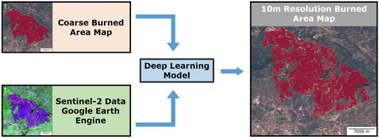
One important limitation of existing algorithms for mapping burned areas with medium to high resolution data is the computational cost and storage required. Even if deep learning techniques reduce the cost of processing the data, just the acquisition and pre-processing of data for an extended period and region can be very slow and challenging for regular desktop or laptop computers. To mitigate this problem, we propose a modular methodology for a faster monitoring of burned areas with 10m resolution. The method explores the storage and processing capacity of the Google Earth Engine (GEE, [23]) for data pre-processing and acquisition, and a deep learning model trained to map the burned areas using previously downloaded pre-fire and post-fire composites. The sequence of steps in our approach consists of: (1) using BA-Net model [13] to produce coarse burned areas maps using VIIRS 375 m bands; (2) splitting the detected burned areas into individual events; (3) downloading pre-fire and post-fire Sentinel-2 composites of red, near-infrared (NIR) and shortwave-infrared (SWIR) only for the regions enclosing the fires of interest, making use of the GEE functionalities to create the pre-fire and post-fire composites; (4) using a deep learning model optimized to generate 10 m burned areas using as inputs the Sentinel-2 data and the coarse burned area map derived from VIIRS.
The proposed approach can be used for a fast monitoring of wildfires as BA-Net model allows for daily updates and Sentinel-2 data are available every 5 days if there is no occlusion by clouds in the burned region. As we will show, the procedure can generate a 10 m resolution burned map for a 1500 hectares fire event in about 5 min overhead time (assuming the coarse mask for the event is already routinely generated and provided) on a regular personal computer, including the download time of the Sentinel-2 data required.
The main objectives of this work are three-fold: (1) To develop a fast and robust tool for quick post-fire assessment, as soon as clean data are available; (2) to allow for a more detailed analysis of historical fires, particularly those with intricate borders between burned and unburned pixels within large fires, and (3) to make the methodology available as a Python package ready to be used.
In line with the third goal of this work, the Python package and pretrained models necessary to apply our methodology are available at https://github.com/mnpinto/FireHR, accessed on 14 April 2021.
2. Data and Methods
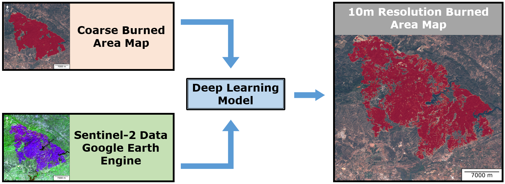
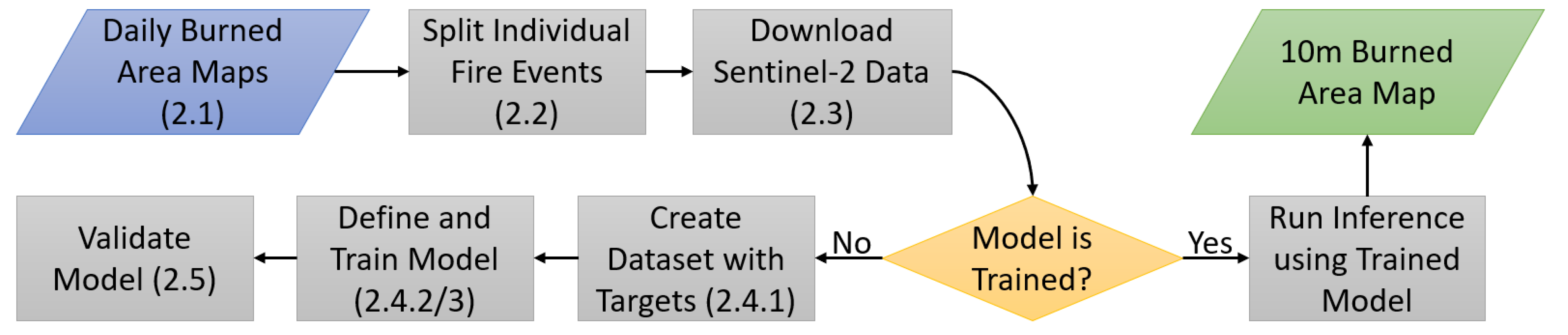
Our study focused on Mediterranean Europe and, since we were working with Sentinel-2A and Sentinel-2B satellites, we were restricted to data from the 2017 fire season onwards. However, in 2017 Portugal’s fire season accounts for a total burned area of about 500,000 hectares, representing more than 50% of the total burned area in the EU for that year [24,25]. Therefore, there was an unusually high amount of data for that year alone that could be used to train and evaluate our model for 10 m resolution burned areas as described in Section 2.4. The pipeline for the approach we propose is illustrated in Figure 1 and described in detail in Section 2.1, Section 2.2, Section 2.3, Section 2.4 and Section 2.5.
2.1. Daily Burned Areas Using BA-Net
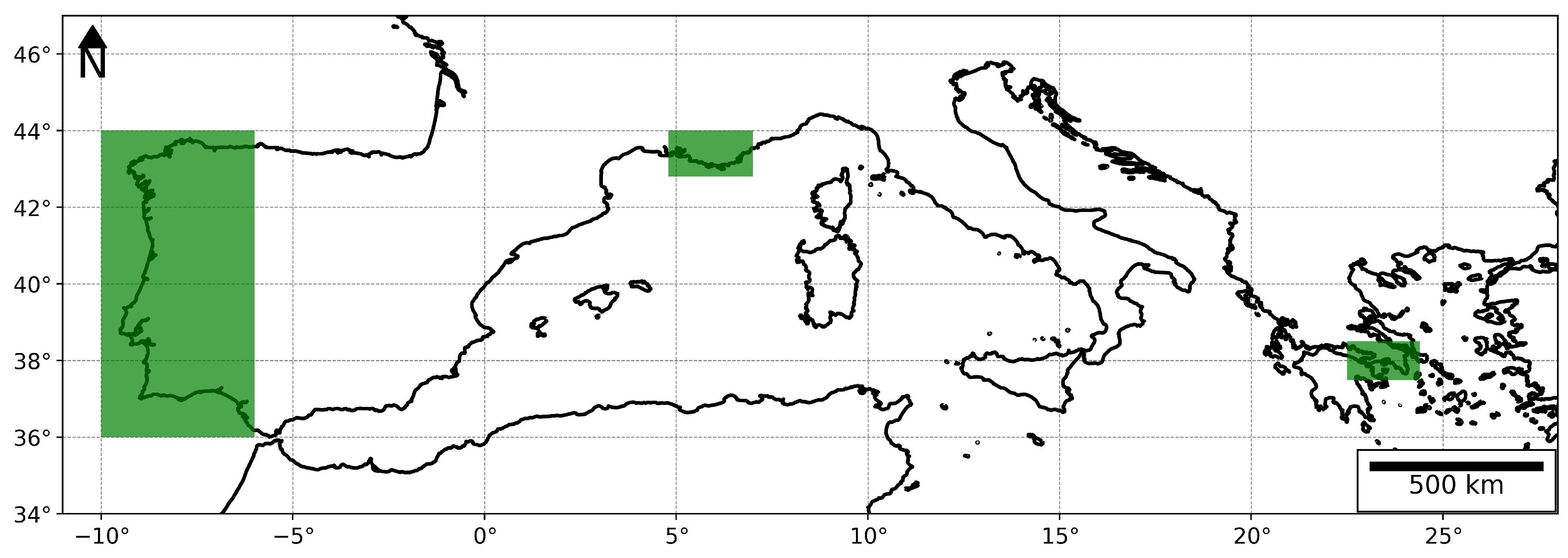
BA-Net [13] is a deep learning model trained to map and date burned areas using sequences of daily satellite images derived from VIIRS sensors. We used the BA-Net Python library version 0.6 (pypi.org/project/banet/0.6.0, accessed on 14 April 2021) to generate the burned area products with 0.001º resolution (about 100 m) for the time periods and regions described in Table 1 and delimited in Figure 2 by green rectangles.
2.2. Split Individual Fire Events
A common method to split individual fire events is flood fill [26,27,28] in which neighbouring burned pixels with identical or sequential date of burning are aggregated to identify the individual burned patches. This method is, however, computationally expensive, particularly for large regions with large fires, and even more if implemented in high-level programming languages (e.g., Python). In order to make the pipeline fast and efficient in Python, we developed the fire_split library (https://github.com/mnpinto/fire_split, accessed on 14 April 2021) that makes use of the very efficient ndimage.label function from SciPy library [29], that split non overlapping patches, enhanced with functionality to allow for a spatial buffer and temporal separation of the events.
The method consists of the following steps:
- 1.
- Create a buffer around the burned pixels using kernel convolution with kernel size pixels;
- 2.
- Use ndimage.label function to split the fires spatially without taking into account the temporal component;
- 3.
- Remove fire events smaller than 25 pixels;
- 4.
- For each retained event, look at the dates of burning and split the event every time the temporal distance is greater than 2 days;
- 5.
- For each newly separated event run ndimage.label to separate events that may have been previously connected by a third one;
- 6.
- Remove again fire events smaller than 25 pixels if any is present after the temporal split.
The value of pixels for the kernel size of the spatial buffer corresponds to a minimum separation distance of about 4 pixels at the 0.001 spatial resolution and was set to be close to, but higher than the original 375 m resolution of the VIIRS data. As for the temporal separation, the value of 2 days was set in order to have a good discrimination of the dense number of fires that occurred in western Iberia in 2017, but still giving enough margin to account for the uncertainty in the date of burning of BA-Net, which is smaller than 2 days for more than 90% of the pixels [13]. The minimum size selected of 25 pixels corresponds to about 25 hectares, a number that is close to about 2 pixels at the original 375 m resolution of the data. In the fire_split Python library all these parameters can be adjusted by the user.
2.3. Sentinel-2 Composites Using Google Earth Engine
Google Earth Engine (GEE) Python API can be used to select, pre-process and download data automatically using a Python script. In fact, in a recent work, Long et al. 2019 ([30]) proposed a global annual burned area mapping tool based on GEE and Landsat images. Our approach significantly differs, as we only use GEE as a pre-processing and data acquisition tool at single event level. In this regard, our method is designed as a tool either for quick post-fire assessment or for a detailed analysis of historical fires. The quick post-fire assessment can be performed as soon as clean Sentinel-2 data are available, i.e., less than 6-days if the following overpass finds clear sky conditions.
Our approach consists in downloading two composites of multispectral images for each event, one corresponding to dates before the fire, and the other immediately after the fire. These images include Sentinel-2 Level-1C (reference code on GEE: COPERNICUS/S2) bands Red (B4), NIR (B8) and SWIR2 (B12). In order to obtain images that are usually free of clouds we computed the median of all available images within the two months prior and after the fire. The Python code we provide has additional options for the pre-processing of the composites, namely, a maximum cloud coverage level can be set to filter cleaner images or the number of images (n) with the least cloud cover fraction could be selected, where n can be set by the user. This pre-processing process, regardless of the option used, is very fast since it was performed on GEE platform. We only download the two (pre-fire and post-fire) composited images for the region of each fire event of interest, as defined with the method described in Section 2.2. Furthermore, as there was a maximum total request size for each download request, we split each fire region into pixel titles that are downloaded individually and then stitched together into the full region image. For the near-real-time monitoring of the fires using our Python code, the post-fire time window can be shortened to select a single image that will be available in less than 6-days after the event, following the best revisit time using both Sentinel-2A and Sentinel-2B. In this case, if clouds and shadows or dense smoke plumes are present over the burned region, the results will be compromised. This is a limitation of any near-real-time application for burned areas.
We note that this approach can also be applied to Landsat data to study events prior to mid-2015 (the date Sentinel 2A became operational). We plan to add this functionality to the Python package in a future update.
2.4. Model and Training
To generate the 10 m burned area maps from Sentinel-2 data and the coarse mask derived from VIIRS data, we used a deep learning model that is defined and trained for such purpose. This sequence of processes (see Figure 1) is described in detail in Section 2.4.1, Section 2.4.2 and Section 2.4.3.
2.4.1. Create Dataset
To train the model we prepared a dataset consisting of events for western Iberia (see Table 1). For each event, the Sentinel-2 data was downloaded using the procedure described in Section 2.3. Since the model training requires batches of data with identically-sized images and the total size is limited by the 8 GB memory of the GPU used for training, large images were cropped into tiles, corresponding to regions of about km. Smaller-sized images were interpolated to fill-in the full tiles.
To train the model with supervision we also needed target data. To generate the targets, we used a semi-automatic approach making use of the pre-fire to post-fire differences of the Normalized Burned Ratio (NBR), a widely used metric to map burned area and estimate burn severity (e.g., [31,32,33]). The approach consisted in the following steps:
- 1.
- NBR was computed for each event using the expression NBR = (NIR − SWIR) / (NIR + SWIR);
- 2.
- The difference of prefire and postfire NBR (dNBR) was computed;
- 3.
- The median dNBR was then computed inside and outside the coarse burned mask, using the BA-Net product;
- 4.
- The dNBR threshold to define the burned region was defined for each event as the mean point between the two medians of step 3;
- 5.
- The resulting mask was cleaned using the method described in Section 2.2 with a spatial buffer of 10 pixels, a minimum pixel size of 100 and keeping only the burned regions representing at least 10% of the total burned area of each event. The choice of the buffer size, minimum pixel size and the 10% criteria was done by visual interpretation with the goal of removing any existing noise around the main burned patch;
- 6.
- Finally, each mask was evaluated visually, together with dNBR data, and events looking “unnatural” were discarded.
This procedure resulted in 3188 input/target pairs of data.
We note that the target masks do not need to be absolutely accurate since the deep learning models, like the one we used (described in the next section) are robust to some degree of random noise [34]. Indeed, during optimization, the model learned how to link the input data to the burned area maps consistently among the training samples, reflecting the spectral patterns associated with burned areas. We stress that users of our Python package do not need to repeat this process as the pre-trained models are provided together with the code.
2.4.2. Define Model
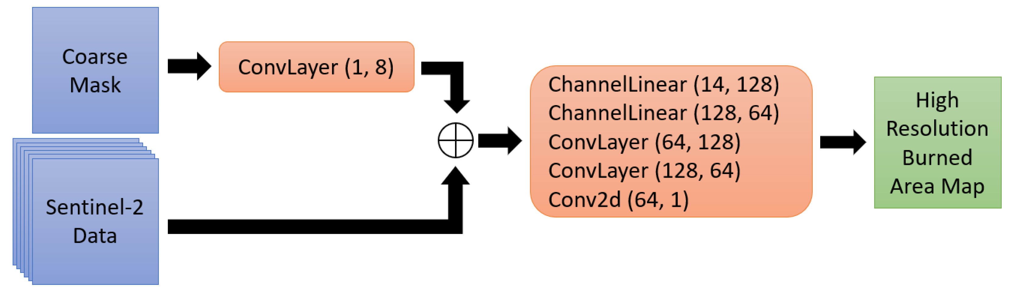
The deep learning model defined to tackle this problem is represented in Figure 3 where numbers in parenthesis indicate the number of input features (left) and the number of output features (right). The ConvLayer is a 2D convolution operation with kernel-size and no bias term, followed by a 2D batch normalization [35] and a Rectified Linear Unit (ReLU, [36]) activation. The rationale for the ConvLayer is that the convolution operation captures local contextual information of close neighbouring pixels, followed by a normalization step that ensures that the data distribution remains with an average close to zero and standard deviation close to one to stabilize the training process in multi-layer models, and finally the rectified linear unit is a commonly used activation function, consisting of setting all negative values to zero and in turn giving the model its non-linear characteristic. The ChannelLinear layer applies a 1D linear layer to the channel dimension (i.e., without awareness of the spatial relation of the pixels) followed by a 1D batch normalization and a ReLU activation. The rationale for the ChannelLinear layers is to combine the features at a pixel level, without any spatial awareness. This allows the model to learn non-linear combinations of the spectral features. For instance, the model could learn a spectral index with characteristics similar to the dNBR described in Section 2.4.1, but since the parameters are learned they result in an optimized index with a 64-dimensional representation, since the number of output features for the second ChannelLinear layer is 64.
The Coarse Mask in Figure 3 is the BA-Net [13] burned area map interpolated to the same projection and spatial resolution as the Sentinel-2 data and after applying a spatial moving average filter with kernel size of pixels (about km) to soften the edges of the coarse mask. The output of the ConvLayer (small orange box in Figure 3) is then concatenated with the 6 input channels of the high-resolution data, corresponding to the Red, NIR and SWIR before and after the fire. The resulting tensor has a size of [batch-size, 14, 512, 512], where the batch-size is constrained by the GPU memory as will be covered in the next subsection. The layers in the large orange block in Figure 3 are then applied sequentially resulting in the high resolution burned area as output, a tensor with size [batch-size, 1, 512, 512].
We also note that by allowing the model to learn an optimal combination of the input bands we can then gain some insight on which input feature has the most impact on the final result, as we will discuss in Section 3.
2.4.3. Train Model
The model was trained using a NVIDIA GTX 1080 GPU. For training, the data were randomly split into a train and validation set with 80/20 ratio, making sure the test events were not in the train set, in order to evaluate if the model was generalizing properly. The model was trained with mixed precision [37] using iterative upscaling starting with 20 epochs at image size and batch-size of 64, followed by 20 epochs at image size and batch-size of 16, and finally by 20 epochs at the original image size and batch-size of 8. Starting with a smaller image size and large batch-size allowed for better stability at the beginning of training, as Batch Normalization is known to be less stable for smaller batch-sizes [38]. For each scale level a one-cycle learning rate schedule [39] was used with a maximum learning rate of 0.01 for the first cycle at scale and dividing the maximum learning rate by the same factor as the batch-size was decreased for the two following cycles, at and scales respectively. The Adam optimizer [40] was used with a weight decay of 0.001. Image augmentations were used to increase the diversity of the dataset, as it is common practice in computer vision applications [41]. The augmentations used were the eight dihedral transformations, brightness, contrast, rotation and wrapping using the default parameters of fastai library [42]. For a general overview of practical deep learning techniques, we recommend fastai open online courses (https://www.fast.ai, accessed on 14 April 2021).
2.5. Validation of the Six Case Studies
For the validation of the six case studies, we used burned area maps produced by the Copernicus Emergency Management Service (CEMS). The CEMS provides on-demand detailed information for several types of emergency situations, including wildfires. The service was activated for all of the six case studies we selected and therefore detailed maps of the burned areas are available. Table 2 describes the details for each CEMS event. For most cases CEMS used SPOT-6-7 1.5 m resolution data. For the “Attica Greece 2” event, CEMS used the higher resolution (0.5 m) Pleiades-1A-1B data to produce the burned area maps. We note, however, that these maps were generated as a quick response to emergency activations and that their level of detail and accuracy may have varied significantly, being dependent on the quality of the source images and on the presence of clouds and/or smoke partially obstructing the view.
For a general overview of the comparison between the two products we also computed the Commission Error (CE), Omission Error (OE) and Dice coefficient, defined as
where TP, FP and FN correspond to the number of pixels for True Positives, False Positives and False Negatives, when considering the CEMS maps as the reference. These are common metrics used to evaluate burned area products (e.g., [15,43]). The rationale for these metrics is that CE (OE) represents the fraction of false positives (negatives) over all predicted (reference) positives and the Dice (also known as F1 score) corresponds to the harmonic mean of precision and recall.
3. Results
3.1. Computation Benchmark
In this section we will present the results and performance benchmarks for six case-studies that took place in the three Mediterranean boxes considered (see Figure 2 and Table 1). For all the computation benchmarks, an Intel i7-7700 CPU or a NVIDIA GTX 1080 GPU were used, running on a machine with 32 GB of RAM. After training the model with the procedure described in Section 2.4.3, the resulting Dice coefficient for the validation set was 0.97.
The first step in our pipeline, the production of the coarse masks using the BA-Net model, can take up to several hours, depending on the size of the region of study and also on the spatial resolution selected for the product. For the benchmark of the BA-Net model, we refer to Pinto et al. 2020 ([13]). Regarding the computational cost to split the fires, the process took about 1 second for French Riviera and Attica Greek regions, since the number of fires was very small. For the western Iberia region, it took about 7 min for 2017 and 2 min for 2018.
The performance benchmarks for the data acquisition and computation of the burned area maps for the six case studies is shown in Table 3. We did not include the time to produce the coarse masks in our performance benchmark, since we are only interested in evaluating the overhead time of generating the 10 m resolution maps. We assume that the coarse product is already routinely generated and provided. The most time-consuming step corresponds to the GEE download process. This step takes less than about 5 min for fires up to about 1500 ha size and, for larger fires, the time increases as expected, since the volume of data to download is significantly larger. Nevertheless, for the largest of the six case studies, a fire with 42,333 ha in central Portugal, the data were downloaded in less than an hour on average. Fires larger than 20,000 ha are rare in Mediterranean Europe and most often only occur in Portugal. The inference time to compute the high resolution burned area map is short, particularly if using a GPU (Table 3 sixth column) which even for the largest fire took less than a minute to compute. For fires under 1500 ha, this step takes 1–2 s on the GPU and about 3 to 6 times more in the CPU. For example, for the 1344 ha fire with ID “French Riviera 2” (Table 3 row 5), the inference time on CPU was 11 s.
3.2. Feature Importance
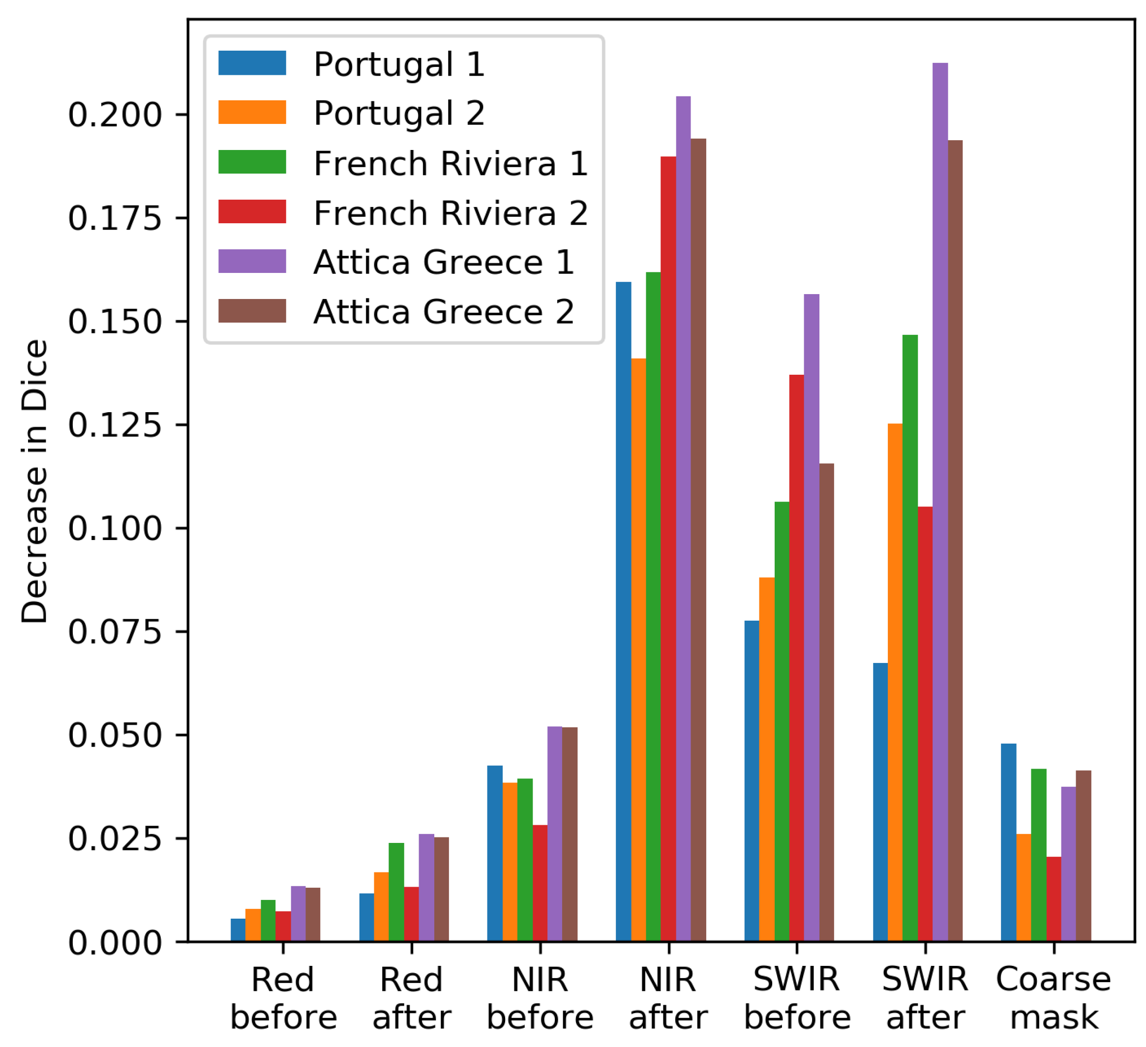
To better understand the results and the trained model we computed the relative importance of each input band to the final result (Figure 4). The relative importance was measured as the decrease in Dice score of the output when the input band in x-axis was randomly shuffled compared to the score when the unchanged input data were used. When shuffling the data, water pixels were masked out to avoid mixing land and water pixels. We can see that, in general, the NIR and SWIR were the most important features (Figure 4), particularly, the post-fire NIR and SWIR followed by the pre-fire SWIR. The pre-fire NIR and coarse mask followed with a small importance variation among the six case studies, and finally the least important feature was the red, particularly the pre-fire red. Looking in more detail at the three dominant features (post-fire SWIR and NIR and pre-fire SWIR), there were noticeable differences among the case studies. For example, while for the “Portugal 1” case the post-fire NIR was the most important feature, for the “Attica Greece 1” case, the post-fire SWIR and NIR showed the highest importance, followed by the pre-fire SWIR. There are several factors that could explain these differences. For example, a fire occurring earlier in a fire season, as is the case for “Portugal 1” event, is more likely to show a stronger drop in NIR as the vegetation is usually not as dry as later in the season. It is also worth noting that our feature importance reflects the spatial variability of the features. If the fire occurs in a perfectly uniform forest region, shuffling the pre-fire features have no impact on the result. In fact, we see that the pre-fire bands, particularly the SWIR were also important, meaning that the location of the burned shape could be to some extent identified before the fire, something that is expected especially for the fires in forest-urban interface regions where the forest-urban delimitation is usually clear in the pre-fire images.
3.3. Case Studies
In this section we look in detail to the six case studies, comparing our product with the CEMS maps to obtain further insight into the performance of our model. Table 4 summarizes the three metrics described in Section 2.5 for each case study. Overall, the agreement between the products is very good with a Dice coefficient greater than 0.92 for all but one event.
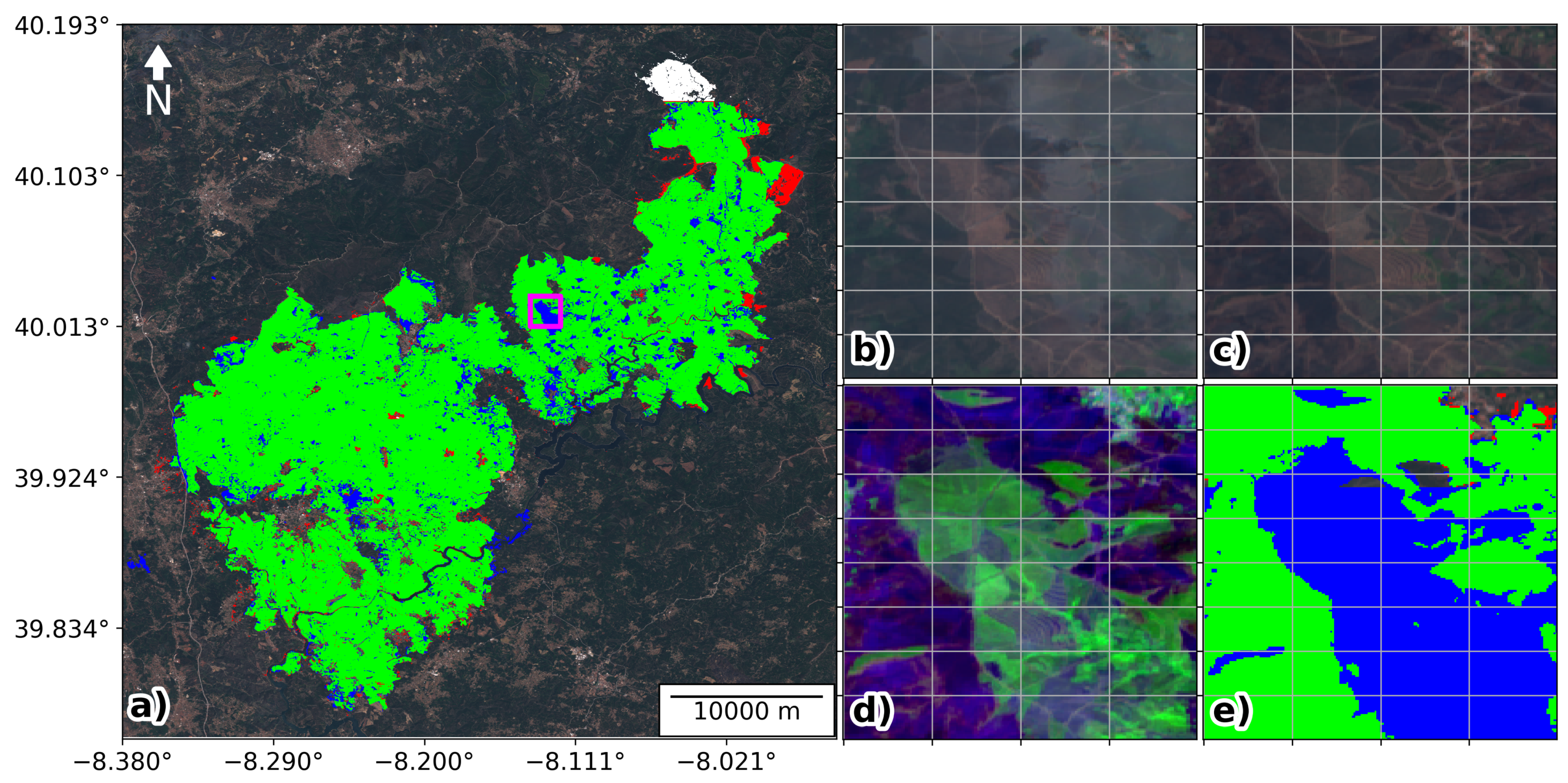
Figure 5 and Figure 6 show the two case studies for Portugal that took place in 2017 and 2018, respectively. The first fire event (Figure 5) occurred in June 2017 in central Portugal and led tragically to a death toll of 64 people [44] and a total burned area of 42,333 ha. The second event (Figure 6) occurred in August 2018 in southwest Portugal, with a total burned area of 23,868 ha and mobilizing up to about 1400 firefighters and 14 aircraft and leading to 41 people injured and millions of euros of economic losses [45].
Figure 5a suggests an overall good accuracy, which was confirmed by a Dice score of 0.933 (Table 4, first row). The white patch on the northeast part of the burned area corresponds to a region not mapped by the CEMS and therefore was not considered for the computation of the evaluation metrics. Regarding the large easternmost red patch, we visually confirmed, using the Sentinel-2 data, that it corresponds to a burned region, but it was one of the latest regions to burn, likely after the CEMS analysis data, thus explaining the difference. On the remaining of the burned region (Figure 5a) we see that most differences lay in small patches within the burned region, which CEMS map attributed to burned contrary to our classification. To get some insight, we looked in detail at one of these patches (identified by a magenta square in Figure 5a) in Figure 5 panels (a) to (e). Looking at panels (b) and (c), corresponding to true colour view median composites for the periods before and after the fire, respectively, we see, although not very clearly, that the green regions in panel (e) had a shift in colour from dark green to dark brown. The false colour composite in panel (d) makes it easier to appreciate this difference. Furthermore, we note that the southernmost section of this burned area was mapped with higher detail by CEMS and Figure 5a shows that the agreement between the two maps is stronger thereby suggesting that most of the differences are in part based on the detail of the analysis or the criteria for regions with a low burn severity as we will further discuss later.
Figure 6 shows once again a very good overall accuracy for the second case study, with a Dice coefficient of 0.928. After the green, the blue colour is the most common in Figure 6a, corresponding to regions where CEMS map assigns pixels as burned contrary to our product. The zoomed region in panels (b) to (e) shows an interesting detail with narrow burned patches captured by our product as well as by CEMS map. It is worth noting that some of the CEMS maps provide burn severity grading but since these varied among the cases, we opted to include all severity grades. As our product does not map different levels of burn severity it is expected that differences may be more frequent in low severity burn regions where the spectral difference in pre-fire to post-fire images was small, as is the case in the example presented in Figure 6.
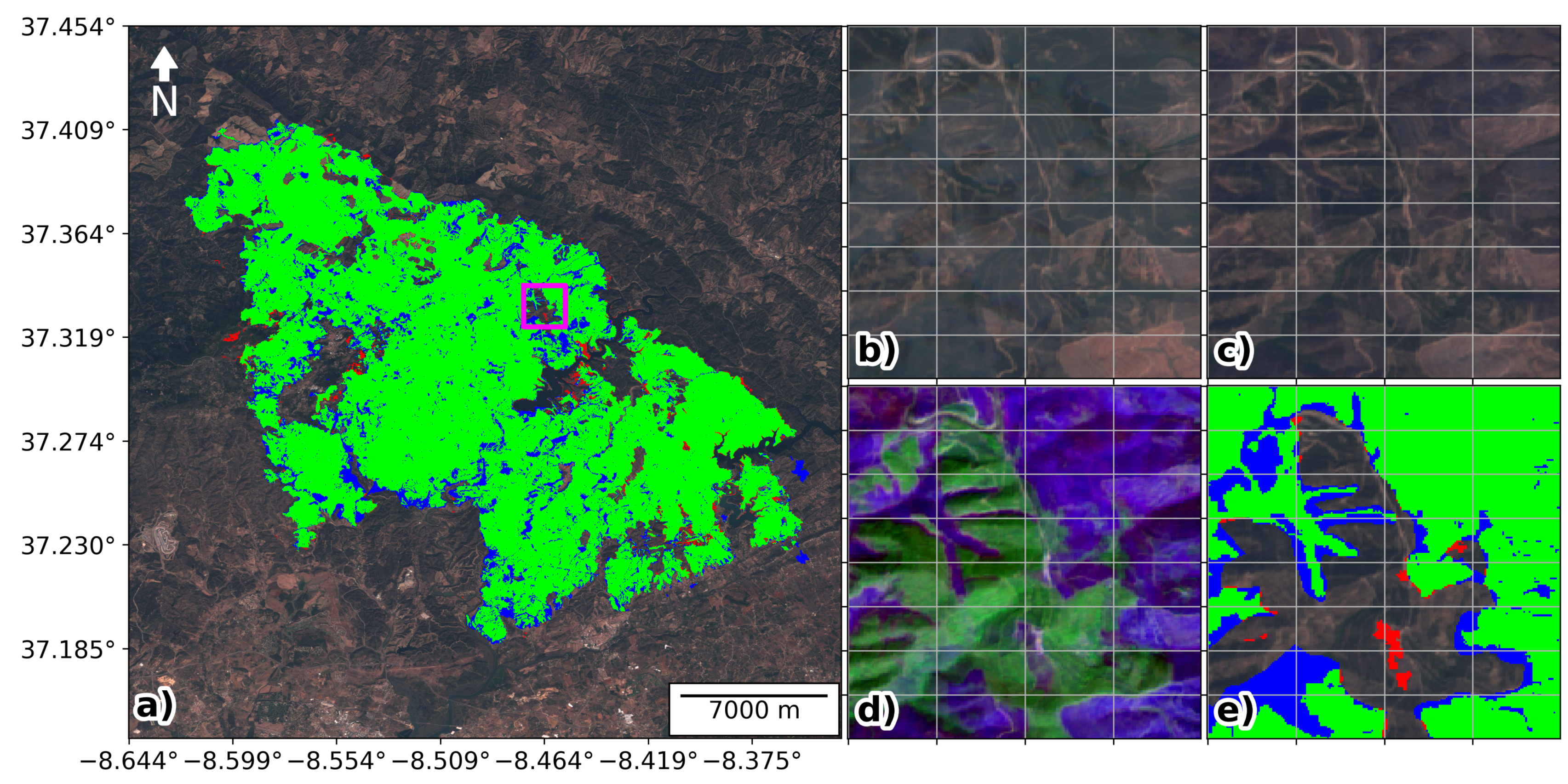
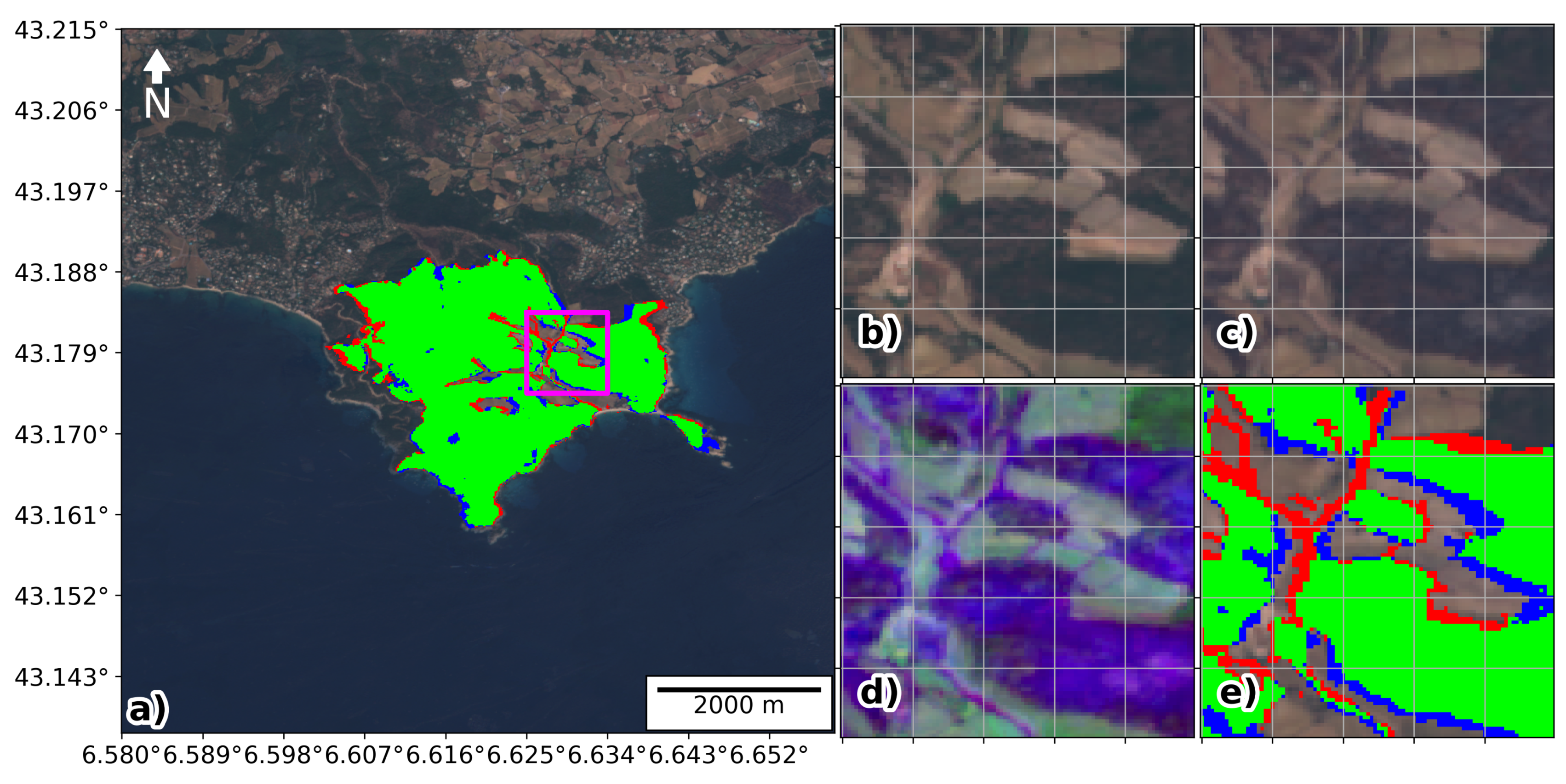
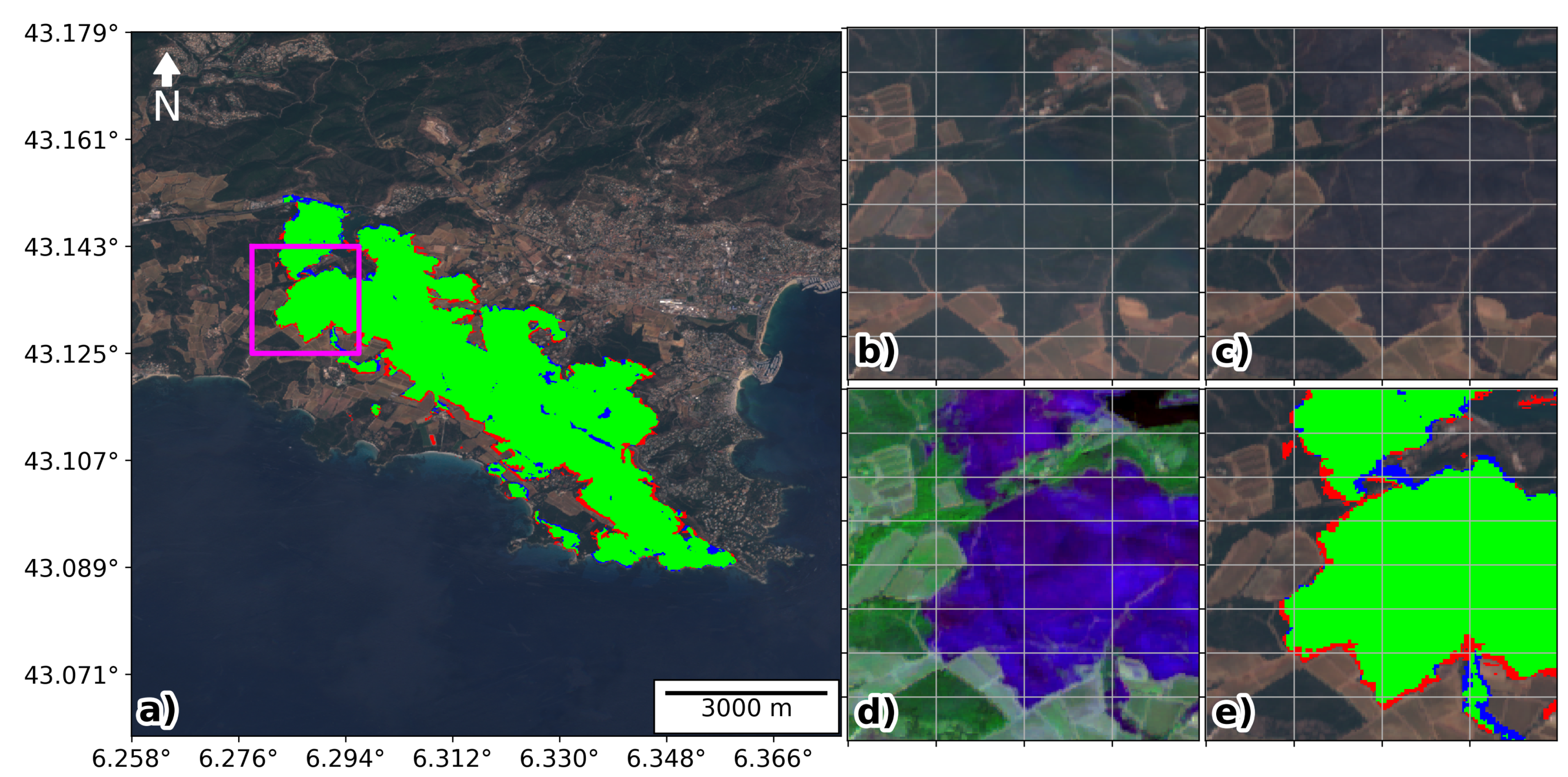
Figure 7 and Figure 8 show the two cases for the French Riviera in July 2017. These two fires represented a total of 489 and 1344 ha of burned area, respectively, and despite being much smaller in size compared to the examples of Portugal, they led to significant socio-economic impacts, forcing the evacuation of more than 10,000 people, according to the local press. The agreement between our product and the CEMS maps was again very good with a Dice coefficient of 0.931 and 0.941 for each case, respectively. The zoomed view in Figure 7 and Figure 8b–e panels shows that the discrepancies between the two maps are mostly in the margins between burned and unburned regions. These small differences are to be expected when comparing products obtained from different satellite sensors, particularly if the raw data have different spatial resolution or view angles.
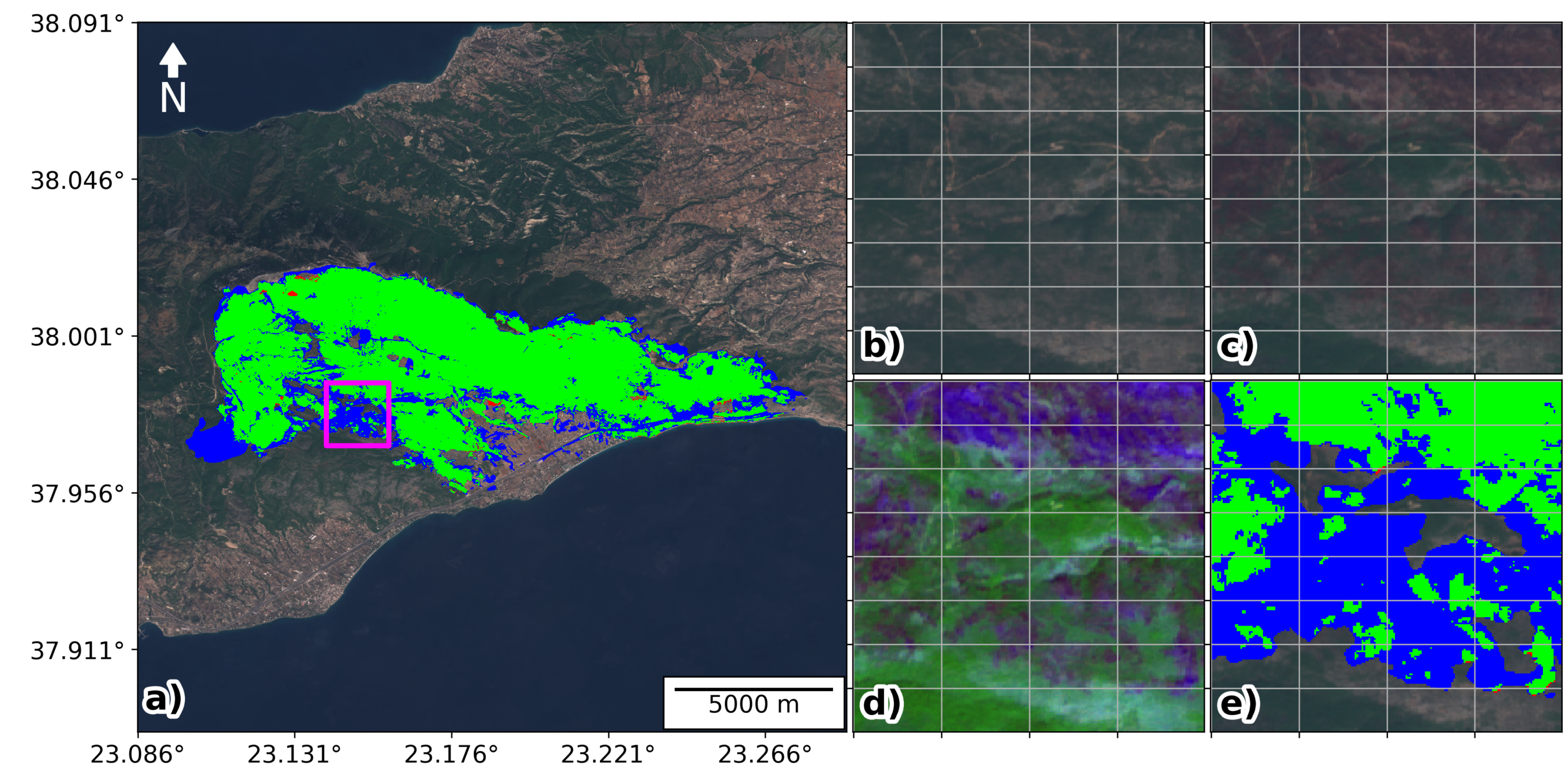
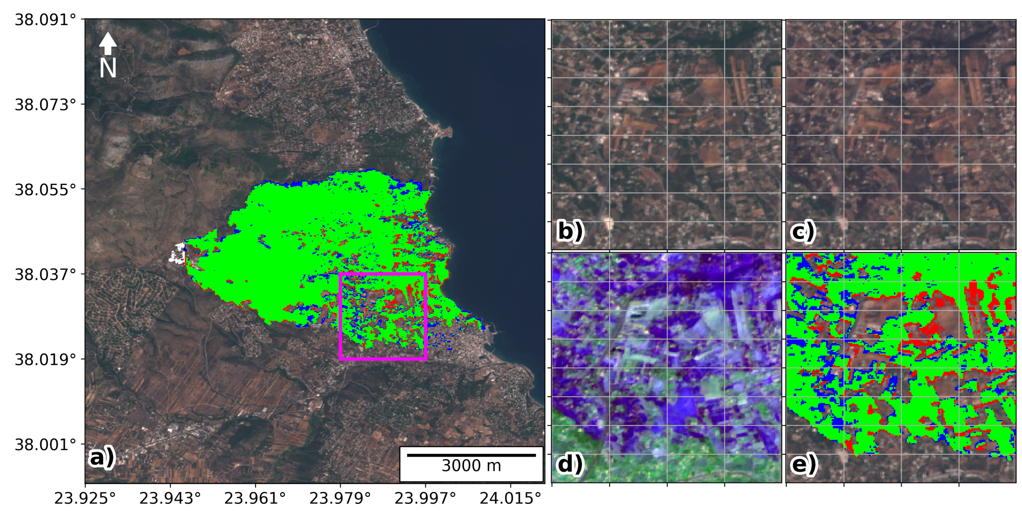
Figure 9 and Figure 10 show the two cases for Attica, Greece in July 2018. The total burned area for these events was 4363 and 1232 ha, respectively. The location of the fires in wildland-urban interfaces together with extreme weather conditions, led to the tragic outcome of 102 fatalities [46]. For these two cases we obtained a Dice coefficient of 0.870 and 0.924, respectively. Starting with the first case (Figure 9) where the discrepancy between our product and the CEMS maps was the largest of all other five case studies considered here, we first note that there is a large blue patch in the western side of the burned area, i.e., a burned scar identified by CEMS maps, contrary to our product. By visually inspecting post-fire Sentinel-2 images we found no evidence for that patch to be burned. It is most likely that this was mis-classified by CEMS due to the presence of clouds in the region as observed in the CEMS data for this case study (see Table 2). Looking now at the zoomed region on Figure 9 panels (b) to (e) we can see that scattered burned patches with sectors that may have burned with a low or negligible severity, since in several parts they still appear in dark green colour in the post-fire true colour composite (panel c). This example illustrates well what we already mentioned in the previous case studies. Looking now at Figure 10 we start by noting that the small white patch on the west side of the burned area is outside the region mapped by CEMS and was therefore not considered to compute the evaluation metrics (Table 4, last row). Focusing now on the zoomed region a high number of small gaps are clearly observed. These correspond to small clusters of houses in the path of the fire and it is therefore a challenging case to map the burned area. We note that for this case the CEMS used data from Pleiades-1A-1B that has a source resolution of 0.5 m. The good agreement between our product and the CEMS is an indication that our methodology can be applied not only for wildland regions but also to more challenging wildland-urban interfaces with as good accuracy, reflecting that the deep learning model described in Section 2.4.2 successfully learned the spectral patterns associated with the burned areas.
4. Discussion
The target data used to train the model are produced with a semi-automatic method and do not correspond to the ground truth, since such reference data do not exist. Often a higher resolution product is used as reference to evaluate the performance of burned area products [47], however, data with a resolution higher than 10 m are usually not available or difficult to obtain. Therefore, the validation is restricted to the six case-studies selected, for which the CEMS burned area maps are available (Table 2). Nevertheless, since the main goal of this work is to provide a fast and practical method (and yet accurate and robust) for a quick monitoring of the burned regions, the comparison with CEMS is very relevant.
Regarding the input data, the coarse mask used in our pipeline is not restricted to be produced by BA-Net model. For instance, it can be manually produced based on ground observations or based on other coarse burned area products. However, the BA-Net product provides daily updates and a state-of-the-art accuracy in the date of burning, making it, to the best of our knowledge, the most appropriate choice for near-real-time applications, when compared to other fully automated products, such as MCD64A1 Collection 6 burned area product ([12]) that can only be produced with at least one month delay. For the higher resolution data, the use of GEE to create the composites and download data at the event level is a major improvement in download time, storage, and processing requirements. This contrasts with the algorithm for near-real-time mapping of burned areas using Sentinel-2 proposed by Pulvirenti et al. 2020 ([48]) for Italy where data is processed at a country level.
Most existing methods for computation of high resolution burned areas are based on indices combining two or more spectral bands, usually Red, NIR and MIR or SWIR, as well as their pre-fire to post-fire difference (e.g., [32,49,50]). In our approach, we used a deep learning model that, instead, learns an optimal non-linear combination of pre-fire and post-fire Red, NIR and SWIR. Furthermore, the convolutional layers that follow allow the model to learn some spatial correlations between neighbouring pixels, instead of considering each pixel individually. This is an important component for burned area identification. Traditional algorithms to map burned areas often rely on a grid expansion method to account for the spatial factor (e.g., [17]). We also note that our deep learning model has about 160,000 parameters, a number that is relatively small for this type of model. This results in lower memory requirements and a faster computation. For instance, typical model architectures for image segmentation, like the U-Net architecture used by Knopp et al. 2020 ([22]), usually have at least millions to tens of millions of parameters. Our smaller model trades off with a lower field of vision (i.e., it can only take into account for close neighboring pixels in the convolutional layers) but we note that: (1) the coarse mask we use as input was generated with a larger model (BA-Net, [13]) and therefore the task of the model we defined for this work (Figure 3) has already a spatial guideline; (2) in the identification of burned areas, the pre-fire to post-fire changes in reflectance are the dominant signal and therefore a very large field of vision is unlikely to be necessary for most situations. This contrasts with other applications of computer vision, where large complex objects need to be identified.
The two main limitations of the methodology proposed are: (1) very small fires may not be captured by the coarse burned area product used as input; (2) for regions where cloud cover is very frequent it may take longer to have clear sky images and therefore the near-real-time mapping is compromised for these situations. These limitations can possibly be addressed in future works by combining multiple input sensors in a single model, in particular through the inclusion of Synthetic Aperture Radar data that is capable of penetrating clouds and smoke [21]. Finally, future research on high resolution burned areas would benefit from detailed ground or drone observations for calibration and validation of the models. This is particularly relevant to generate very high resolution burned severity maps where information at single tree scale may be relevant.
5. Conclusions
Forest fires have long been part of the Mediterranean landscape and will continue to be so in the future. Climate change only worsens this problem as the meteorological conditions for severe fires become more and more likely in a warming scenario [3,4]. In this context, having the tools for a timely high-resolution assessment of the burned areas is of paramount importance. Satellite data are now openly available allowing anyone to access high quality data. Powerful computational tools, such as the Google Earth Engine (GEE), make the visualization and processing of high volumes of data feasible. Our proposed method corresponds to a fast and yet reliable tool, suited for monitoring of burned areas with 10m resolution, leveraging the functionalities of GEE as a data acquisition and pre-processing tool to obtain input data to then feed to a deep learning model that outputs the burned area map. This methodology can generate a burned map for a 1500 ha fire in about 5 min, using about 25 MB of storage on disk and running inference on a computer with an 8-core processor and 8 GB of RAM. This is important for researchers, forest managers, or any entity interested in studying or evaluating the impacts of wildland fires. We showed in this work, six case studies as examples of application of the proposed methodology. A visual evaluation of the maps produced by our model and the validation using maps produced by the CEMS shows how our model successfully captures the fine details of the burned areas that cannot be observed in coarse resolution products. This is especially noticeable in fires occurring in wildland-urban interfaces where the fine spatial resolution is decisive to identify small clusters of houses. By using a deep learning model that maps the pre-fire and post-fire Red, NIR and SWIR bands, together with the coarse resolution mask, to the final 10 m resolution burned map, we can then study how each input band affects the result on the trained model. The results show that, as expected, the NIR and SWIR bands are the most important spatial features. On average post-fire NIR shows the highest importance, followed by post-fire SWIR, pre-fire SWIR and pre-fire NIR. There are however differences among the case studies that are likely due to the spatial and temporal context in which the fire occurred. Finally, this work is a step towards a fully automated procedure to produce high resolution burned areas in near-real-time over an extended region with a feasible computational cost. Once again, the code to our methodology is provided as a Python package, ready to apply to new cases, at https://github.com/mnpinto/FireHR, accessed on 14 April 2021.
Author Contributions
Conceptualization, M.M.P., R.M.T., I.F.T. and C.C.D.; data curation, M.M.P.; formal analysis, M.M.P.; funding acquisition, R.M.T., I.F.T. and C.C.D.; investigation, M.M.P.; methodology, M.M.P., R.M.T., I.F.T. and C.C.D.; project administration, R.M.T., I.F.T. and C.C.D.; resources, R.M.T., I.F.T. and C.C.D.; software, M.M.P.; supervision, R.M.T., I.F.T. and C.C.D.; validation, M.M.P.; visualization, M.M.P.; writing—original draft, M.M.P., R.M.T., I.F.T. and C.C.D.; writing—review and editing, M.M.P., R.M.T., I.F.T. and C.C.D. All authors have read and agreed to the final version of the manuscript and accept responsibility for its content.
Funding
This work was in part supported by Fundação para a Ciência e a Tecnologia, Portugal (FCT) under project FireCast (PCIF/GRF/0204/2017). Miguel M. Pinto was supported by FCT through the PhD grant PD/BD/142779/2018. Ricardo M. Trigo contribution was partially supported with funding from the European Union (EU) and in-kind funding from FCiências.ID/FCUL within the frame of the ERANET “European Research Area for Climate Services—ERA4CS” 2016 Call (INDECIS—ERA4CS—GA 690462).
Institutional Review Board Statement
Not applicable.
Informed Consent Statement
Not applicable.
Data Availability Statement
All data used for this research is publicly available. Sentinel-2 data was obtained from Google Earth Engine https://earthengine.google.com/, accessed on 14 April 2021. VIIRS data was obtained from Level-1 and Atmosphere Archive and Distribution System Distributed Active Archive Center https://ladsweb.modaps.eosdis.nasa.gov/, accessed on 14 April 2021. Validation data was obtained from Copernicus Emergency Management Service https://emergency.copernicus.eu, accessed on 14 April 2021. Trained model parameters and code are available at https://github.com/mnpinto/FireHR, accessed on 14 April 2021.
Conflicts of Interest
The authors declare no conflict of interest. The funders had no role in the design of the study; in the collection, analyses, or interpretation of data; in the writing of the manuscript, or in the decision to publish the results.
References
- Pausas, J.G.; Llovet, J.; Rodrigo, A.; Vallejo, R. Are wildfires a disaster in the Mediterranean basin?—A review. Int. J. Wildland Fire 2008, 17, 713. [Google Scholar] [CrossRef]
- Bowman, D.M.J.S.; Williamson, G.J.; Abatzoglou, J.T.; Kolden, C.A.; Cochrane, M.A.; Smith, A.M.S. Human exposure and sensitivity to globally extreme wildfire events. Nat. Ecol. Evol. 2017, 1. [Google Scholar] [CrossRef] [PubMed]
- Turco, M.; Rosa-Cánovas, J.J.; Bedia, J.; Jerez, S.; Montávez, J.P.; Llasat, M.C.; Provenzale, A. Exacerbated fires in Mediterranean Europe due to anthropogenic warming projected with non-stationary climate-fire models. Nat. Commun. 2018, 9. [Google Scholar] [CrossRef]
- Ruffault, J.; Curt, T.; Moron, V.; Trigo, R.M.; Mouillot, F.; Koutsias, N.; Pimont, F.; Martin-StPaul, N.; Barbero, R.; Dupuy, J.L.; et al. Increased likelihood of heat-induced large wildfires in the Mediterranean Basin. Sci. Rep. 2020, 10. [Google Scholar] [CrossRef] [PubMed]
- Fernandez-Manso, A.; Quintano, C.; Roberts, D.A. Burn severity influence on post-fire vegetation cover resilience from Landsat MESMA fraction images time series in Mediterranean forest ecosystems. Remote Sens. Environ. 2016, 184, 112–123. [Google Scholar] [CrossRef]
- Hislop, S.; Jones, S.; Soto-Berelov, M.; Skidmore, A.; Haywood, A.; Nguyen, T. Using Landsat Spectral Indices in Time-Series to Assess Wildfire Disturbance and Recovery. Remote Sens. 2018, 10, 460. [Google Scholar] [CrossRef] [Green Version]
- Freire, J.G.; DaCamara, C.C. Using cellular automata to simulate wildfire propagation and to assist in fire management. Nat. Hazards Earth Syst. Sci. 2019, 19, 169–179. [Google Scholar] [CrossRef] [Green Version]
- Loepfe, L.; Lloret, F.; Román-Cuesta, R.M. Comparison of burnt area estimates derived from satellite products and national statistics in Europe. Int. J. Remote Sens. 2011, 33, 3653–3671. [Google Scholar] [CrossRef]
- Mangeon, S.; Field, R.; Fromm, M.; McHugh, C.; Voulgarakis, A. Satellite versus ground-based estimates of burned area: A comparison between MODIS based burned area and fire agency reports over North America in 2007. Anthr. Rev. 2015, 3, 76–92. [Google Scholar] [CrossRef] [Green Version]
- Chuvieco, E.; Mouillot, F.; van der Werf, G.R.; Miguel, J.S.; Tanase, M.; Koutsias, N.; García, M.; Yebra, M.; Padilla, M.; Gitas, I.; et al. Historical background and current developments for mapping burned area from satellite Earth observation. Remote. Sens. Environ. 2019, 225, 45–64. [Google Scholar] [CrossRef]
- Chuvieco, E.; Lizundia-Loiola, J.; Pettinari, M.L.; Ramo, R.; Padilla, M.; Tansey, K.; Mouillot, F.; Laurent, P.; Storm, T.; Heil, A.; et al. Generation and analysis of a new global burned area product based on MODIS 250m reflectance bands and thermal anomalies. Earth Syst. Sci. Data 2018, 10, 2015–2031. [Google Scholar] [CrossRef] [Green Version]
- Giglio, L.; Boschetti, L.; Roy, D.P.; Humber, M.L.; Justice, C.O. The Collection 6 MODIS burned area mapping algorithm and product. Remote Sens. Environ. 2018, 217, 72–85. [Google Scholar] [CrossRef]
- Pinto, M.M.; Libonati, R.; Trigo, R.M.; Trigo, I.F.; DaCamara, C.C. A deep learning approach for mapping and dating burned areas using temporal sequences of satellite images. ISPRS J. Photogramm. Remote Sens. 2020, 160, 260–274. [Google Scholar] [CrossRef]
- Humber, M.L.; Boschetti, L.; Giglio, L.; Justice, C.O. Spatial and temporal intercomparison of four global burned area products. Int. J. Digit. Earth 2018, 12, 460–484. [Google Scholar] [CrossRef]
- Roteta, E.; Bastarrika, A.; Padilla, M.; Storm, T.; Chuvieco, E. Development of a Sentinel-2 burned area algorithm: Generation of a small fire database for sub-Saharan Africa. Remote Sens. Environ. 2019, 222, 1–17. [Google Scholar] [CrossRef]
- Bastarrika, A.; Chuvieco, E.; Martín, M.P. Mapping burned areas from Landsat TM/ETM + data with a two-phase algorithm: Balancing omission and commission errors. Remote Sens. Environ. 2011, 115, 1003–1012. [Google Scholar] [CrossRef]
- Stroppiana, D.; Bordogna, G.; Carrara, P.; Boschetti, M.; Boschetti, L.; Brivio, P. A method for extracting burned areas from Landsat TM/ETM+ images by soft aggregation of multiple Spectral Indices and a region growing algorithm. ISPRS J. Photogramm. Remote Sens. 2012, 69, 88–102. [Google Scholar] [CrossRef]
- Hawbaker, T.J.; Vanderhoof, M.K.; Beal, Y.J.; Takacs, J.D.; Schmidt, G.L.; Falgout, J.T.; Williams, B.; Fairaux, N.M.; Caldwell, M.K.; Picotte, J.J.; et al. Mapping burned areas using dense time-series of Landsat data. Remote Sens. Environ. 2017, 198, 504–522. [Google Scholar] [CrossRef]
- Drusch, M.; Del Bello, U.; Carlier, S.; Colin, O.; Fernandez, V.; Gascon, F.; Hoersch, B.; Isola, C.; Laberinti, P.; Martimort, P.; et al. Sentinel-2: ESA’s optical high-resolution mission for GMES operational services. Remote Sens. Environ. 2012, 120, 25–36. [Google Scholar] [CrossRef]
- Filipponi, F. Exploitation of Sentinel-2 Time Series to Map Burned Areas at the National Level: A Case Study on the 2017 Italy Wildfires. Remote Sens. 2019, 11, 622. [Google Scholar] [CrossRef] [Green Version]
- Ban, Y.; Zhang, P.; Nascetti, A.; Bevington, A.R.; Wulder, M.A. Near Real-Time Wildfire Progression Monitoring with Sentinel-1 SAR Time Series and Deep Learning. Sci. Rep. 2020, 10. [Google Scholar] [CrossRef] [PubMed] [Green Version]
- Knopp, L.; Wieland, M.; Rättich, M.; Martinis, S. A Deep Learning Approach for Burned Area Segmentation with Sentinel-2 Data. Remote Sens. 2020, 12, 2422. [Google Scholar] [CrossRef]
- Gorelick, N.; Hancher, M.; Dixon, M.; Ilyushchenko, S.; Thau, D.; Moore, R. Google Earth Engine: Planetary-scale geospatial analysis for everyone. Remote Sens. Environ. 2017, 202, 18–27. [Google Scholar] [CrossRef]
- San-Miguel-Ayanz, J.; Durrant, T.; Boca, R.; Libertà, G.; Branco, A.; de Rigo, D.; Ferrari, D.; Maianti, P.; Vivancos, T.A.; Costa, H.; et al. Forest fires in Europe. Middle East N. Afr. 2017, 2018. [Google Scholar] [CrossRef]
- Turco, M.; Jerez, S.; Augusto, S.; Tarín-Carrasco, P.; Ratola, N.; Jiménez-Guerrero, P.; Trigo, R.M. Climate drivers of the 2017 devastating fires in Portugal. Sci. Rep. 2019, 9. [Google Scholar] [CrossRef]
- Archibald, S.; Roy, D.P. Identifying individual fires from satellite-derived burned area data. In Proceedings of the 2009 IEEE International Geoscience and Remote Sensing Symposium, Cape Town, South Africa, 12–17 July 2009. [Google Scholar] [CrossRef]
- Nogueira, J.; Ruffault, J.; Chuvieco, E.; Mouillot, F. Can We Go Beyond Burned Area in the Assessment of Global Remote Sensing Products with Fire Patch Metrics? Remote Sens. 2016, 9, 7. [Google Scholar] [CrossRef] [Green Version]
- Laurent, P.; Mouillot, F.; Yue, C.; Ciais, P.; Moreno, M.V.; Nogueira, J.M.P. FRY, a global database of fire patch functional traits derived from space-borne burned area products. Sci. Data 2018, 5. [Google Scholar] [CrossRef] [Green Version]
- Virtanen, P.; Gommers, R.; Oliphant, T.E.; Haberland, M.; Reddy, T.; Cournapeau, D.; Burovski, E.; Peterson, P.; Weckesser, W.; Bright, J.; et al. SciPy 1.0: Fundamental algorithms for scientific computing in Python. Nat. Methods 2020, 17, 261–272. [Google Scholar] [CrossRef] [Green Version]
- Long, T.; Zhang, Z.; He, G.; Jiao, W.; Tang, C.; Wu, B.; Zhang, X.; Wang, G.; Yin, R. 30 m Resolution Global Annual Burned Area Mapping Based on Landsat Images and Google Earth Engine. Remote Sens. 2019, 11, 489. [Google Scholar] [CrossRef] [Green Version]
- Cocke, A.E.; Fulé, P.Z.; Crouse, J.E. Comparison of burn severity assessments using Differenced Normalized Burn Ratio and ground data. Int. J. Wildland Fire 2005, 14, 189. [Google Scholar] [CrossRef] [Green Version]
- Miller, J.D.; Thode, A.E. Quantifying burn severity in a heterogeneous landscape with a relative version of the delta Normalized Burn Ratio (dNBR). Remote Sens. Environ. 2007, 109, 66–80. [Google Scholar] [CrossRef]
- Quintano, C.; Fernández-Manso, A.; Fernández-Manso, O. Combination of Landsat and Sentinel-2 MSI data for initial assessing of burn severity. Int. J. Appl. Earth Obs. Geoinf. 2018, 64, 221–225. [Google Scholar] [CrossRef]
- Rolnick, D.; Veit, A.; Belongie, S.; Shavit, N. Deep learning is robust to massive label noise. arXiv 2017, arXiv:1705.10694. [Google Scholar]
- Ioffe, S.; Szegedy, C. Batch normalization: Accelerating deep network training by reducing internal covariate shift. In Proceedings of the International Conference on Machine Learning, PMLR, Lille, France, 7–9 July 2015; pp. 448–456. [Google Scholar]
- Nair, V.; Hinton, G.E. Rectified linear units improve restricted boltzmann machines. In Proceedings of the 27th International Conference on International Conference on Machine Learning, Haifa, Israel, 21–24 June 2010. [Google Scholar]
- Micikevicius, P.; Narang, S.; Alben, J.; Diamos, G.; Elsen, E.; Garcia, D.; Ginsburg, B.; Houston, M.; Kuchaiev, O.; Venkatesh, G.; et al. Mixed precision training. arXiv 2017, arXiv:1710.03740. [Google Scholar]
- Wu, Y.; He, K. Group Normalization. In Computer Vision—ECCV 2018; Springer: Munich, Germany, 2018; pp. 3–19. [Google Scholar] [CrossRef]
- Smith, L.N. A disciplined approach to neural network hyper-parameters: Part 1–learning rate, batch size, momentum, and weight decay. arXiv 2018, arXiv:1803.09820. [Google Scholar]
- Kingma, D.P.; Ba, J. Adam: A method for stochastic optimization. arXiv 2014, arXiv:1412.6980. [Google Scholar]
- Shorten, C.; Khoshgoftaar, T.M. A survey on Image Data Augmentation for Deep Learning. J. Big Data 2019, 6. [Google Scholar] [CrossRef]
- Howard, J.; Gugger, S. Fastai: A Layered API for Deep Learning. Information 2020, 11, 108. [Google Scholar] [CrossRef] [Green Version]
- Padilla, M.; Stehman, S.V.; Ramo, R.; Corti, D.; Hantson, S.; Oliva, P.; Alonso-Canas, I.; Bradley, A.V.; Tansey, K.; Mota, B.; et al. Comparing the accuracies of remote sensing global burned area products using stratified random sampling and estimation. Remote Sens. Environ. 2015, 160, 114–121. [Google Scholar] [CrossRef] [Green Version]
- Pinto, M.M.; DaCamara, C.C.; Trigo, I.F.; Trigo, R.M.; Turkman, K.F. Fire danger rating over Mediterranean Europe based on fire radiative power derived from Meteosat. Nat. Hazards Earth Syst. Sci. 2018, 18, 515–529. [Google Scholar] [CrossRef] [Green Version]
- DaCamara, C.C.; Libonati, R.; Pinto, M.M.; Hurduc, A. Near- and Middle-Infrared Monitoring of Burned Areas from Space. In Satellite Information Classification and Interpretation; IntechOpen: London, UK, 2019. [Google Scholar] [CrossRef] [Green Version]
- Lagouvardos, K.; Kotroni, V.; Giannaros, T.M.; Dafis, S. Meteorological Conditions Conducive to the Rapid Spread of the Deadly Wildfire in Eastern Attica, Greece. Bull. Am. Meteorol. Soc. 2019, 100, 2137–2145. [Google Scholar] [CrossRef]
- Boschetti, L.; Roy, D.; Justice, C. International Global Burned Area Satellite Product Validation Protocol Part I–Production and Standardization of Validation Reference Data; Committee on Earth Observation Satellites: Maryland, MD, USA, 2009; pp. 1–11. [Google Scholar]
- Pulvirenti, L.; Squicciarino, G.; Fiori, E.; Fiorucci, P.; Ferraris, L.; Negro, D.; Gollini, A.; Severino, M.; Puca, S. An Automatic Processing Chain for Near Real-Time Mapping of Burned Forest Areas Using Sentinel-2 Data. Remote Sens. 2020, 12, 674. [Google Scholar] [CrossRef] [Green Version]
- Escuin, S.; Navarro, R.; Fernández, P. Fire severity assessment by using NBR (Normalized Burn Ratio) and NDVI (Normalized Difference Vegetation Index) derived from LANDSAT TM/ETM images. Int. J. Remote Sens. 2007, 29, 1053–1073. [Google Scholar] [CrossRef]
- Libonati, R.; DaCamara, C.C.; Pereira, J.M.C.; Peres, L.F. On a new coordinate system for improved discrimination of vegetation and burned areas using MIR/NIR information. Remote Sens. Environ. 2011, 115, 1464–1477. [Google Scholar] [CrossRef]
Figure 1.
Pipeline to generate the 10 m resolution burned areas. Numbers in parenthesis indicate the paper’s subsection describing the process.
Figure 1.
Pipeline to generate the 10 m resolution burned areas. Numbers in parenthesis indicate the paper’s subsection describing the process.

Figure 2.
Green rectangles delimit the regions of study described in Table 1.
Figure 2.
Green rectangles delimit the regions of study described in Table 1.

Figure 3.
Diagram representing the model pipeline. Blue, orange, and green boxes represent inputs, neural network modules and outputs, respectively. The ⨁ symbol indicates that features are concatenated on the channel dimension. Numbers in parenthesis indicate the number of input (left) and output (right) features for the respective neural network layer.

Figure 4.
Feature importance for each input channel measured before and after the fire (x-axis) and per fire event (indicated by the top label).
Figure 4.
Feature importance for each input channel measured before and after the fire (x-axis) and per fire event (indicated by the top label).

Figure 5.
Visual analysis of “Portugal 1” fire. Panel (a) shows the true colour satellite view for the selected fire region together with the burned area maps derived in this study and by CEMS: green represents the pixels where both products agree; red represent burned pixels identified by this study and not by CEMS; blue corresponds to burned pixels identified by CEMS and not in this study; white pixels correspond to burned pixels outside the CEMS mapping window. Panels (b–e) correspond to the zoomed region indicated by the magenta square in panel (a); panels (b,c) represent the true colour view for the median composite before and after the fire, respectively; panels (d,e) show the false colour composite of pre/post-fire differences in red, NIR and SWIR and the zoomed view of panel (a) map, respectively.

Figure 6.
Visual analysis of “Portugal 2” fire. See Figure 5 for panel descriptions.
Figure 6.
Visual analysis of “Portugal 2” fire. See Figure 5 for panel descriptions.

Figure 7.
Visual analysis of “French Riviera 1” fire. See Figure 5 for panel descriptions.
Figure 7.
Visual analysis of “French Riviera 1” fire. See Figure 5 for panel descriptions.

Figure 8.
Visual analysis of “French Riviera 2” fire. See Figure 5 for panel descriptions.
Figure 8.
Visual analysis of “French Riviera 2” fire. See Figure 5 for panel descriptions.

Figure 9.
Visual analysis of “Attica Greece 1” fire. See Figure 5 for panel descriptions.
Figure 9.
Visual analysis of “Attica Greece 1” fire. See Figure 5 for panel descriptions.

Figure 10.
Visual analysis of “Attica Greece 2" fire. See Figure 5 for panel descriptions.
Figure 10.
Visual analysis of “Attica Greece 2" fire. See Figure 5 for panel descriptions.


Table 1.
Study regions details.
| Region Name | Bounding Box | Time | Use |
|---|---|---|---|
| Western Iberia | 36.0 to 44.0N 10.0 to 6.0W | June to October 2017 and August 2018 | Train/Test |
| French Riviera | 42.8 to 44.0N 4.8 to 7.0E | July 2017 | Test |
| Attica Greece | 37.5 to 38.5N 22.5 to 24.4E | July 2018 | Test |
Table 2.
Description of the CEMS validation data for the six test regions.
| FireID | CEMS ID | Source Name | Source Resolution | Published Time (UTC) |
|---|---|---|---|---|
| Portugal 1 | EMSR207 | SPOT-6-7/Other | 1.5 m/Other | 2017-06-22 19:56:12 |
| Portugal 2 | EMSR303 | SPOT-6-7 | 1.5 m | 2018-08-10 17:00:48 |
| French Riviera 1 | EMSR214 | SPOT-6 | 1.5 m | 2017-07-31 14:58:03 |
| French Riviera 2 | EMSR214 | SPOT-6 | 1.5 m | 2017-07-28 19:16:39 |
| Attica Greece 1 | EMSR300 | SPOT-6-7 | 1.5 m | 2018-07-30 17:28:17 |
| Attica Greece 2 | EMSR300 | Pleiades-1A-1B | 0.5 m | 2018-07-26 16:38:00 |
Table 3.
Benchmark results for the six test regions. Computation times are the average of seven runs for all cases but GEE Download Time that corresponds to the average of three runs in different days.
Table 3.
Benchmark results for the six test regions. Computation times are the average of seven runs for all cases but GEE Download Time that corresponds to the average of three runs in different days.
| FireID | Sentinel-2 mage Size | Sentinel-2 Data Size on Disk | GEE Download Time | Inference Time (CPU) | Inference Time (GPU) | Burned Area (ha) |
|---|---|---|---|---|---|---|
| Portugal 1 | 4733 × 4732 | 300 MB | 51 min | 152 s | 50 s | 42,333 |
| Portugal 2 | 3419 × 3418 | 161 MB | 25 min | 76 s | 21 s | 23,868 |
| French Riviera 1 | 870 × 881 | 9 MB | 3 min | 5 s | 1 s | 489 |
| French Riviera 2 | 1315 × 1327 | 19 MB | 4 min | 11 s | 2 s | 1344 |
| Attica Greece 1 | 2262 × 2260 | 62 MB | 13 min | 32 s | 7 s | 4363 |
| Attica Greece 2 | 1093 × 1081 | 16 MB | 4 min | 7 s | 1 s | 1232 |
Table 4.
Evaluation metrics for the six test regions considering the CEMS product as the reference.
| FireID | Commission Error | Omission Error | Dice |
|---|---|---|---|
| Portugal 1 | 0.034 | 0.097 | 0.933 |
| Portugal 2 | 0.016 | 0.122 | 0.928 |
| French Riviera 1 | 0.074 | 0.065 | 0.931 |
| French Riviera 2 | 0.072 | 0.047 | 0.941 |
| Attica Greece 1 | 0.007 | 0.225 | 0.870 |
| Attica Greece 2 | 0.059 | 0.093 | 0.924 |
Publisher’s Note: MDPI stays neutral with regard to jurisdictional claims in published maps and institutional affiliations. |
© 2021 by the authors. Licensee MDPI, Basel, Switzerland. This article is an open access article distributed under the terms and conditions of the Creative Commons Attribution (CC BY) license (https://creativecommons.org/licenses/by/4.0/).
Share and Cite
MDPI and ACS Style
Pinto, M.M.; Trigo, R.M.; Trigo, I.F.; DaCamara, C.C. A Practical Method for High-Resolution Burned Area Monitoring Using Sentinel-2 and VIIRS. Remote Sens. 2021, 13, 1608. https://0-doi-org.brum.beds.ac.uk/10.3390/rs13091608
AMA Style
Pinto MM, Trigo RM, Trigo IF, DaCamara CC. A Practical Method for High-Resolution Burned Area Monitoring Using Sentinel-2 and VIIRS. Remote Sensing. 2021; 13(9):1608. https://0-doi-org.brum.beds.ac.uk/10.3390/rs13091608
Chicago/Turabian StylePinto, Miguel M., Ricardo M. Trigo, Isabel F. Trigo, and Carlos C. DaCamara. 2021. "A Practical Method for High-Resolution Burned Area Monitoring Using Sentinel-2 and VIIRS" Remote Sensing 13, no. 9: 1608. https://0-doi-org.brum.beds.ac.uk/10.3390/rs13091608
Note that from the first issue of 2016, this journal uses article numbers instead of page numbers. See further details here.