Robust Controller for Pursuing Trajectory and Force Estimations of a Bilateral Tele-Operated Hydraulic Manipulator

Abstract

In hazardous/emergency situations, public safety is of the utmost concern. In areas where human access is not possible or is restricted due to hazardous situations, a system or robot that can be distantly controlled is mandatory. There are many applications in which force cannot be applied directly while using physical sensors. Therefore, in this research, a robust controller for pursuing trajectory and force estimations while deprived of any signals or sensors for bilateral tele-operation of a hydraulic manipulator is suggested to handle these hazardous, emergency circumstances. A terminal sliding control with a sliding perturbation observer (TSMCSPO) is considered as the robust controller for a coupled leader and hydraulic follower system. The ultimate use of this controller is as a sliding perturbation observer (SPO) that can estimate the reaction force without any physical force sensors. Robust and perfect position tracking is attained with terminal sliding mode control (TSMC) in addition to control of the hydraulic follower manipulator. The force estimation and pursuing trajectory for the leader–follower system is built upon a bilateral tele-operation control approach. The difference between the reaction forces (caused by the remote environment) and the operating forces (applied by the human operator) required the involvement of an impedance model. The impedance model is implemented in the leader manipulator to provide human operators with an actual sense of the reaction force while the manipulator connects with the remote environment. A camera is used to ensure the safety of the workplace through visual feedback. The experimental results showed that the controller was robust at pursuing trajectory and force estimations for the bilateral tele-operation control of a hydraulic manipulator.

1. Introduction

The modern world requires an uninterrupted source of electrical energy for sustainable development; for this, nuclear power plants (NPP) are a promising energy resource option. The operational lifespan of nuclear power plants is around 40–65 years [1]. Consequently, upon the completion of its life cycle, the nuclear power plant must be decommissioned properly. Decommissioning of a nuclear power plant mainly involves the clean-up of all the residual radioactive waste materials. This residual waste emits an energy known as radiation, which is proven to be extremely fatal for humans [2]. The concentrated amount of radioactive emission makes the dismantling process highly unsafe for a human workforce. Consequently, the involvement of a human workforce must be minimized for the sake of their health and safety. Robots can be considered as an alternative solution [2] to safely complete the clean-up jobs.

The dismantling process consists of several steps (i.e., transportation, storage of waste products, dismantling the structure, disposing of radioactive material, etc.). It is evident from the previous research works that countless robot-equipped decommissioning facilities are operating successfully [3]. An early use of robots was reported in 1979 at three miles’ island after an accidental meltdown of the nuclear reactor. Several tasks were performed remotely by what was at that time considered a novel vision system [4]. LaserSnake2 developed by OCRobotics is another robot that is being widely used as an assistive laser cutter in power plant dismantling operations [5]. However, nuclear dismantling sites often have constrained spaces and are highly polluted facilities. In such highly contaminated and constrained spaces, fully independent solutions may not be considered safe and cost-effective in the near future. A fully autonomous robot may turn out to actually increase the risk factors, rather than provide a helping hand.

Bilateral control with tele-operation systems creates a combination of human abilities with the benefits of accurate, repetitive, and cost-effective robotic manipulation. As a result, assistive tele-operation systems for dismantling and characterizing nuclear power plants could be viable solutions. Previously, several research works have suggested the usefulness of bilateral control systems in performing such activities. For example, the authors in [6,7,8] proposed bilateral tele-operation systems in different areas including environments simulated virtually, space exploration, and robotic assistance in (minimally) invasive surgery. Lovasz and co-workers [8] proposed the use of hepatic exoskeletons for tele-operations in outer space. Similarly, Ozaki et al. [9] proposed an algorithm based on a force sensor to sense the interaction forces (position and orientation of wrist) to increase the efficiency of human operations with a tele-operated system.

Several studies previously described that if the interaction force between the follower manipulator and its surrounding is controlled by a human operator, the overall efficiency and performance of the system may increase [9,10,11]. The authors of [12] proposed a bilateral control method with six degrees of freedom (DOF) for surgical applications. Mejía et al. [13] addressed the control issue of a leader–follower based tele-operation system by proposing a coupling matrix that converted the error dynamics into linear and nonlinear parts that satisfied the matching condition. Later, they used this representation to design discontinuous casual controllers to achieve bilateral coordination both in force and in time.

In the last few years, approaches that estimate interaction forces have been extensively used. Murakami and co-workers [14] proposed a torque sensor-free control for a manipulator with multi-DOF. In addition, the researchers developed a disturbance observer for estimating external reaction force with specified assumptions of gravity and friction efforts. In [15], the researchers considered an effectual disturbance observer by utilizing the feedback of a sensor-less observer, which could instantly estimate the reaction force, and a stable force control was realized. The use of a follower manipulator’s inverse dynamics to detect the contact forces in a tele-operated (minimally) invasive surgical system was also proposed [16]. In [17], researchers proposed a force/torque observer based on two different neural-networks. A promising accuracy of 98.3% was demonstrated for human hand-force and environment-contact estimation. To effectively detect the reaction forces in a bilateral tele-operation system, an observer based on a Kalman filter was proposed in [18]. In 2016, Aviles et al. [19] proposed a novel vision-based approach to detect the contacting forces in a surgery using an assistive robot. However, the applicability of the vision-based methods to detect the contacting forces is often restricted due to low precision and accuracy of the visual measurements.

Kallu et al. [20] measured the reaction force for a dual-armed robotic manipulator by virtue of model control with a sliding-perturbation-observer (SMCSPO). However, in their research, the authors did not used any force/torque sensors. The same SMCSPO method was used for the estimation of the reaction force of a hydraulic manipulator in [21]. SMCSPO has previously been proven as an effective and accurate control scheme to estimate perturbation in the control of a surgical robot and a hydraulic robot manipulator [21,22,23,24,25,26]. For example, in [27], the authors used the sliding mode while fabricating the regulator to compensate for the nonlinearities introduced in the actuators. Several recent studies have shown a considerable improvement for dealing with nonlinearities based on a similar approach [28,29,30]. The purpose of these estimations are to minimize the chattering from the output of system by exploiting perturbation compensation. Additionally, in [31], the authors used a sliding mode controller to calculate an approximation of the reaction force of a bilateral tele-operation system.

Similarly, Cao and co-workers [32] addressed the problem of tracking the position and estimating the state of a robotic manipulator with a hybrid approach. Two techniques, neural network and TSMC, were applied by the authors. Specifically, the neural network was used to estimate the system dynamics and TSMC was applied to estimate the position and the velocity of system. The methodology was validated using a simulation analysis. Likewise, another variant of TSMC was used for position tracking of a three-DOF hydraulic manipulator in [31]. Xuan et al. [33] also used a slightly modified version of TSMC for tracking the trajectory of a hydraulic manipulator with three DOF.

Based on the prior outcomes, we proposed a terminal sliding-mode control with a sliding perturbation observer (TSMCSPO) for pursuing trajectory and force estimations for the bilateral tele-operation of a hydraulic manipulator. The strategic structure competently follows the trajectory and the estimate of the reaction forces of the leader–follower robotic-arm in addition to bi-lateral tele-operation control of the leader/follower manipulator based on the hydraulic manipulator. In our work, by implementing the sliding perturbation observer (SPO), we estimated the reaction force of the hydraulic follower manipulator. A precise and effective tracking of the position and force was achieved via the bilateral tele-operation control system suggested in this study. While designing the bilateral tele-operation control system, the difference between the follower system’s reaction forces and the leader system’s applied forces was considered with the impedance model. Here, it should be noted that the reaction force is the actual effect of the hydraulic follower manipulator in remote environments. On the other hand, additionally, the applied force of the leader system is the force an operator generates. The results presented in this research effectively show the summary of trajectory tracking of both position and force with high accuracy.

The remainder of the manuscript is organized as follow: Section 2 defines the dynamics of the hydraulic manipulator. Section 3 deals with the TSMCSPO theory and the algorithm to estimate reaction force. Afterwards, Section 4 outlines the bilateral tele-operation control method. Section 5 and Section 6, respectively, summarize the experimental setup and the corresponding results. Finally, concluding observations about the research are presented in Section 7.

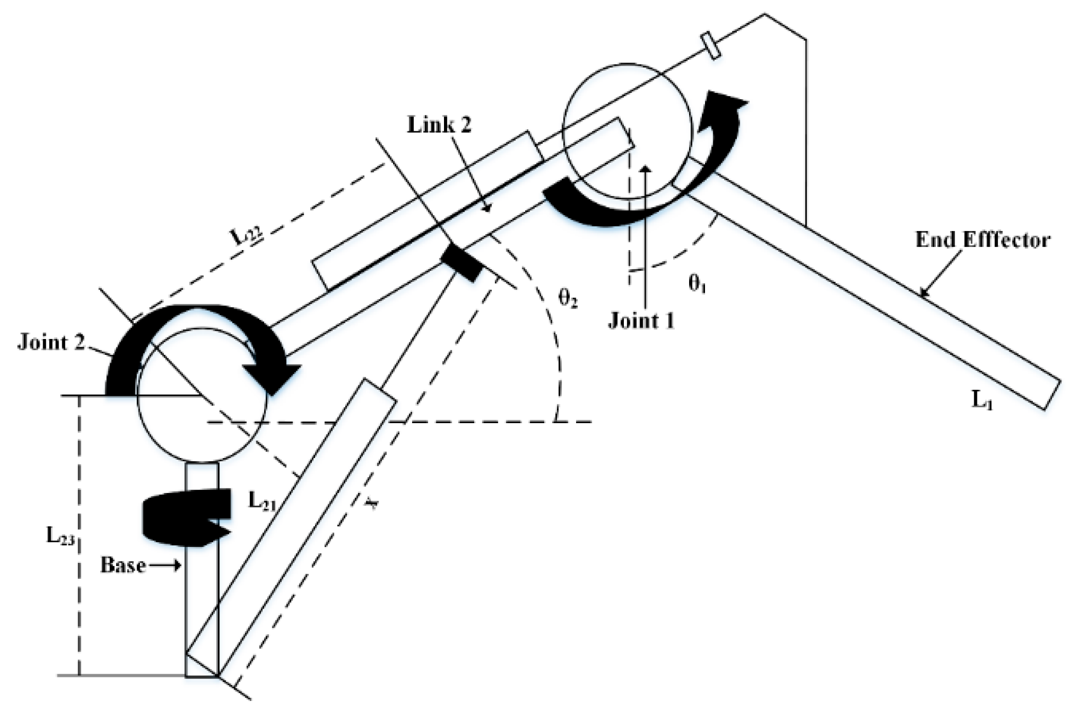
2. Dynamics of the Hydraulic Manipulator

Hydraulic manipulators have been commonly used for handling and as machine tools in various industries over the past few decades. A schematic diagram of a three-DOF articulated hydraulic manipulator developed to dismantle an NPP is shown in Figure 1.

The dynamics of the manipulator characterize the relationship between the applied forces, the resultant torques generated by the applied forces, and the final motion due to the torques. The basic equation demonstrating the robot dynamics in free space is given below

$$T=A\left(\theta \right)\ddot{\theta }+B\left(\theta ,\dot{\theta }\right)+g\left(\theta \right)$$

(1)

where $T$, $\theta$ and $A\left(\theta \right),B\left(\theta ,\dot{\theta }\right),g\left(\theta \right)$ are joint torques, joint angles, the inertia matrix, the centrifugal torque, and the joint space gravity task, respectively. Each link of the hydraulic-servo-system can be articulated mathematically [34].

$$\begin{array}{r}(J_{s1}+\Delta J_{s1})\cdot {\dot{\theta }}_1+(D_{s1}+\Delta D_{s1}+\beta )\cdot {\dot{\theta }}_1\\ +0.5\cdot M_{s1}\cdot g\cdot L_{s1}\cdot \sin {\theta }_1+{\tau }_{e1}=T_1\end{array}$$

(2)

$$\begin{array}{r}(J_{s2}+\Delta J_{s2})\cdot {\ddot{\theta }}_2+(D_{s2}+\Delta D_{s2})\cdot {\dot{\theta }}_2\\ +0.5M_{s2}\cdot g\cdot L_2\cdot \sin {\theta }_2+{\tau }_{e2}=T_2\end{array}$$

(3)

$$\begin{array}{r}(J_{s3}+\Delta J_{s3})\cdot {\ddot{\theta }}_3+(D_{s3}+\Delta D_{s3})\cdot {\dot{\theta }}_3\\ +0.5M_{s3}\cdot g\cdot L_3\cdot \sin {\theta }_3+{\tau }_{e3}=T_3\end{array}$$

(4)

In Equations (2)–(4), $J$ is the inertia and $D$ is the damping value. Specifically, $J_{s1}$, $J_{s2}$, $J_{s3}$, $D_{s1}$, $D_{s2}$, and $D_{s3}$, respectively, define the inertia and damping of the base, second link, and end effector. Additionally, ${\beta }_1$, ${\beta }_2$, represents the viscosity of each cylinder and $M_{s1}$, $M_{s2}$, and $M_{s3}$ represent masses of the base, second link, and end effector, respectively. The term Δ defines the uncertainty in these equations. The length of the base and end effector is expressed by $L_1$ and $L_3$, $L_2$ represents the length from the center-of-mass (COM) of the second link, ${\tau }_{e1}$, ${\tau }_{e2}$, and ${\tau }_{e3}$ represent the reaction torque generated by contact with the environment and joints 1, 2, and 3, respectively, $\lambda$ represents the dynamical effect of the base, ${\dot{\theta }}_1$ and $\dot{x}$ represent the viscosity friction of cylinder 1 and cylinder 2, respectively, and $T_1$, $T_2$, $T_3$ are joint torques of the base, second link, and end effector.

3. Terminal Sliding Mode Control with Sliding Perturbation Observer (TSMCSPO)

3.1. Terminal Sliding Mode Control (TSMC)

The terminal sliding mode control (TSMC) relates the terminal sliding surfaces in the reaching phase and the sliding phase for robotic manipulators with global finite-time stability [35]. To explain the robustness of these kinds of control algorithms, the Lyapunov stability theory is best suited and also provides extra features related to precision. The TSMC can be expressed as a nonlinear differential equation of the first order of the form:

$$s_j={\dot{e}}_j+{\beta }_j{\left|e_j\right|}^{r}sign\left(e_j\right)=0$$

(5)

In Equation (5), the $sign\left(e_j\right)$ is a sign function of $e_j$, ${\beta }_j>0$, $0<r<1$, and $e_j=x_{1j}-x_{1dj}$ is the actual position tracking error. An appropriate form that assures the presence of the TSMC can be expressed as:

$$\frac{1}{2}\frac{d}{dt}{s}^2\le -\eta \left|s\right|; \eta >0$$

(6)

which guarantee $\left|s\left(T_r\right)\right|-\left|s\left(0\right)\right|>-\eta T_r$. $T_r$ is the reaching time which fulfills $T_r=\left|s\left(0\right)\right|/\eta$. Sliding dynamics are defined as follows.

$${\dot{s}}_j=-{\eta }_{1j}sign(s_j)-{\eta }_{2j}{\left|s_j\right|}^{r}sign(s_j)$$

(7)

where ${\eta }_{1j}$, ${\eta }_{2j}$ are greater than zero and ${\eta }_{1j}>\left|{\psi }_j\right|$. The system control for maneuvering is described as

$$\begin{array}{r}{u}_j=B^{-1}Col({\ddot{x}}_{1dj}+f_j(\mathbf{x})+{\beta }_{j}r{\left|e_j\right|}^{r-1}{\dot{e}}_j\\ -{\eta }_{1j}sign(s_j)-{\eta }_{2j}{\left|s_j\right|}^{r}sign(s_j){)}_j\end{array}$$

(8)

Previously, Han et al. [36] explained that when the control approaches the sliding surface, $s_j=0$, the control input of Equation (8) will become non-singular. However, the singular function shall occur in the case of $s_j\ne 0$, with ${\dot{e}}_j\ne 0$ and $e=0$. To avoid the existence of the singular function, the below equation must be satisfied:

$${\left|\dot{e}\right|}^r=\{\begin{array}{cc}r{\left|\dot{e}\right|}^{r-1}\dot{e},\hfill & if \dot{e}\ne 0, e\ne 0\hfill \\ r{|\Delta |}^{r-1}\dot{e},\hfill & if \dot{e}\ne 0, e\ne 0\hfill \\ 0,\hfill & if \dot{e}\ne 0, e\ne 0\hfill \end{array}$$

(9)

The authors of [37] confirmed the asymptotic stability of TSMCSPO.

3.2. Sliding Perturbation Observer (SPO)

The authors of [38] specified a momentary outline of perturbation. Sliding perturbation observer (SPO) is a permutation of an SO (sliding observer) and a perturbation observer. The SO is an observer that can estimate the state of an uncertain non-linear system. The state-space of the jth link in a second-order system can be signified as:

$$\begin{array}{l}{\dot{x}}_{1j}=x_{2j}\\ {\dot{x}}_{2j}=f_j(\mathbf{x})+\underset{i=1}{\overset{n}{\Sigma }}{b}_{ji}\left(\widehat{\mathbf{x}}\right)u_i+{\psi }_j(\mathbf{x},t)\\ y_j=x_{1j}\end{array}$$

(10)

In Equation (10), ${\psi }_j(\mathbf{x},t)$ signifies perturbation. The estimate of state variables is arithmetically stated as,

$$\begin{array}{l}{\dot{\widehat{x}}}_{1j}={\widehat{x}}_{2j}\\ {\dot{\widehat{x}}}_{2j}=f_j(\widehat{\mathbf{x}})+\underset{i=1}{\overset{n}{\Sigma }}{b}_{ji}\left(\widehat{\mathbf{x}}\right)u_i+{\widehat{\psi }}_j(\mathbf{x},t)\end{array}$$

(11)

Likewise, ${\widehat{\psi }}_j(\mathbf{x},t)$ signifies estimation of perturbation. A new control variable is defined to de-couple the control input for the estimation of perturbation and is described as,

$$f_j\left(\widehat{\mathbf{x}}\right)+\underset{i=1}{\overset{n}{\Sigma }}{b}_{ji}\left(\widehat{\mathbf{x}}\right)u_i={\alpha }_{3j}{\overline{u}}_j$$

(12)

where ${\alpha }_3>0$, ${\overline{u}}_{}$ is new control variable. Hence, the control input might be arithmetically stated as,

$$\mathbf{u}=B^{-1}Col[{\alpha }_{3j}{\overline{u}}_j-f_j\left(\widehat{\mathbf{x}}\right)]$$

(13)

where $\mathbf{u}={\left[u_1\dots u_n\right]}^T$ and $B={\left[b_{ji}\left(\widehat{\mathbf{x}}\right)\right]}_{n\times n}$. The difference of $b_{ji}\left(\widehat{\mathbf{x}}\right)$ and $b_{ji}\left(\mathbf{x}\right)$ is actually part of $\Delta b_{ji}$. Lastly, the state dynamics corresponding to the transformation defined in Equation (14) are

$${\ddot{x}}_j={\alpha }_{3j}{\overline{u}}_j+{\psi }_j$$

(14)

Moura et al. [39] provided imitative SPO mathematical equations as,

$${\dot{\widehat{x}}}_{1j}={\widehat{x}}_{2j}-k_{1j}sat({\tilde{x}}_{1j})$$

(15)

$${\dot{\widehat{x}}}_{2j}={\alpha }_3{\overline{u}}_j-k_{2j}sat({\tilde{x}}_{1j})+{\widehat{\Psi }}_j$$

(16)

$${\dot{\widehat{x}}}_{3j}={\alpha }_{3j}^2\left({\overline{u}}_j+{\alpha }_{3j}{\widehat{x}}_{2j}-{\widehat{x}}_{3j}\right)$$

(17)

$${\widehat{\mathit{\psi }}}_j={\alpha }_{3j}({\alpha }_3{\widehat{x}}_{2j}-{\widehat{x}}_{3j})$$

(18)

$$sat({\tilde{x}}_{1j})=\{\begin{array}{c}{\tilde{x}}_{1j}/\left|{\tilde{x}}_{1j}\right|,if\left|{\tilde{x}}_{1j}\right|\ge {\epsilon }_{0j}\\ {{\tilde{x}}_{1j}/\epsilon }_{0j},if\left|{\tilde{x}}_{1j}\right|\le {\epsilon }_{0j}\end{array}$$

(19)

Slotine et al. [40] described the $sat({\tilde{x}}_{1j})$ as the structure for anti-chattering and the TSMC controller boundary layer was denoted by ${\epsilon }_{0j}$. The estimation error of the measurable state and positive numbers are $\tilde{x}=\widehat{x}-x$, $k_{1j}$, $k_{2j}$, respectively. Finally, the error-dynamics of the SPO are established as,

$${\dot{\tilde{x}}}_{1j}={\tilde{x}}_{2j}-k_{1j}sat({\tilde{x}}_{1j})$$

(20)

$${\dot{\tilde{x}}}_{2j}=-k_{2j}sat({\tilde{x}}_{1j})+{\tilde{\Psi }}_j$$

(21)

$${\dot{\tilde{x}}}_{3j}=-{\alpha }_{3j}^2\left({\alpha }_{3j}{\tilde{x}}_{2j}-{\tilde{x}}_{3j}\right)+\dot{\Psi }/{\alpha }_{3j}$$

(22)

The dynamics of ${\tilde{x}}_{2j}$, as an outcome of SPO shall establish

$${\dot{\tilde{x}}}_{2j}+\left(k_{2j}/k_{1j}\right){\tilde{x}}_{2j}={\tilde{\Psi }}_j$$

(23)

The interaction of the frequency-domain between (b/w) ${\tilde{\Psi }}_j$ and ${\Psi }_j$ is mathematically represented as follow

$${\tilde{\Psi }}_j\left(p\right)=\frac{p\left[p^2+\left(k_{1j}/{\epsilon }_{0j}\right)p+k_{2j}/{\epsilon }_{0j}\right]}{p^3+\left(k_{1j}/{\epsilon }_{0j}\right)p^2+\left(k_{1j}/{\epsilon }_{0j}\right)p+{\alpha }_{3j}^2\left(k_{2j}/{\epsilon }_{0j}\right)}\left(-{\Psi }_j\left(p\right)\right)$$

(24)

The above defined function in Equation (24) is nothing but a high-pass filter that represents the relation between actual and error perturbation. Equation (24) indicates that the estimated perturbation will be correct as the value of the perturbation is less than the range of low frequency.

3.3. Terminal Sliding Mode Control with Sliding Perturbation Observer (TSMCSPO)

By combining the controller (TSMC) and an observer (SPO), a new robust controller is formed, which is called the terminal sliding mode control with sliding perturbation observer (TSMCSPO) [37]. The error ${\widehat{e}}_j$ between the required (expected) trajectories with estimation values is reduced by using the controller (TSMC). The ${\widehat{s}}_j$ dynamics are described by

$${\widehat{s}}_j={\dot{\widehat{e}}}_j+{\beta }_{j1}{\left|{\widehat{e}}_j\right|}^{r}sign\left(\widehat{e}\right)$$

(25)

where ${\widehat{e}}_j={\widehat{x}}_{1j}-x_{1dj}$ is the estimated position tracking error. The suitable presence state of TSMCSPO can be insured by designing ${\dot{\widehat{s}}}_j$ as

$${\dot{\widehat{s}}}_j=-{\Gamma }_j{R}_{\max j}\left(k_{1j}/{\epsilon }_{0j}\right)sign({\widehat{s}}_j)-{\eta }_{3j}{\left|s_j\right|}^{r}sign({\widehat{s}}_j)$$

(26)

where ${\Gamma }_j$ is the perturbation of the anticipated boundary, ${\eta }_{3j}>0$, and $R_{\max j}$ is described as follows:

$$R_{\max j}=\frac{p\left[p+\left(k_{1j}/{\epsilon }_{0j}\right)\right]}{p^3+\left(k_{1j}/{\epsilon }_{0j}\right)p^2+\left(k_{2j}/{\epsilon }_{0j}\right)p+{\alpha }_{3j}^2\left(k_{2j}/{\epsilon }_{0j}\right)}$$

(27)

The control input ${\overline{u}}_j$ for the corresponding TSMCSPO is as follows:

If ${\widehat{x}}_{2j}-\left(k_{1j}/{\epsilon }_{0j}\right){\tilde{x}}_{1j}-{\dot{x}}_{1dj}\ne 0,\widehat{e}\ne 0$,

$${\overline{u}}_j=\frac{1}{{\alpha }_{3j}}\left\{\begin{array}{l}-{\Gamma }_j{R}_{\max j}\left(k_{1j}/{\epsilon }_{0j}\right)sign({\widehat{s}}_j)-{\eta }_{3j}{\left|s_j\right|}^{r}sign(\widehat{s})+\\ \left[k_{2j}/{\epsilon }_{0j}-{\left(k_{1j}/{\epsilon }_{0j}\right)}^2\right]{\tilde{x}}_{1j}+{\ddot{x}}_{1dj}-{\widehat{\Psi }}_j-\\ {\beta }_{j}r{\left|{\widehat{e}}_j\right|}^{r-1}\left({\widehat{x}}_{2j}-\left(k_{1j}/{\epsilon }_{0j}\right){\tilde{x}}_{1j}-{\dot{x}}_{1dj}\right)\end{array}\right\}$$

(28)

If ${\widehat{x}}_{2j}-\left(k_{1j}/{\epsilon }_{0j}\right){\tilde{x}}_{1j}-{\dot{x}}_{1dj}\ne 0,\widehat{e}=0$,

$${\overline{u}}_j=\frac{1}{{\alpha }_{3j}}\left\{\begin{array}{l}-{\Gamma }_j{R}_{\max j}\left(k_{1j}/{\epsilon }_{0j}\right)sign({\widehat{s}}_j)-{\eta }_{3j}{\left|s_j\right|}^{r}sign(\widehat{s})+\\ \left[k_{2j}/{\epsilon }_{0j}-{\left(k_{1j}/{\epsilon }_{0j}\right)}^2\right]{\tilde{x}}_{1j}+{\ddot{x}}_{1dj}-{\widehat{\Psi }}_j-\\ {\beta }_{j}r{|\Delta |}^{r-1}\left({\widehat{x}}_{2j}-\left(k_{1j}/{\epsilon }_{0j}\right){\tilde{x}}_{1j}-{\dot{x}}_{1dj}\right)\end{array}\right\}$$

(29)

If ${\widehat{x}}_{2j}-\left(k_{1j}/{\epsilon }_{0j}\right){\tilde{x}}_{1j}-{\dot{x}}_{1dj}=0$,

$${\overline{u}}_j=\frac{1}{{\alpha }_{3j}}\left\{\begin{array}{l}-{\Gamma }_j{R}_{\max j}\left(k_{1j}/{\epsilon }_{0j}\right)sign({\widehat{s}}_j)-{\eta }_{3j}{\left|s_j\right|}^{r}sign(\widehat{s})+\\ \left[k_{2j}/{\epsilon }_{0j}-{\left(k_{1j}/{\epsilon }_{0j}\right)}^2\right]{\tilde{x}}_{1j}+{\ddot{x}}_{1dj}-{\widehat{\Psi }}_j\end{array}\right\}$$

(30)

Thus, the $s_j$ dynamics encircled by boundary $\left|{\widehat{s}}_j\right|\le {\epsilon }_{0j}$ are

$$\begin{array}{l}{\dot{s}}_j+\left({\eta }_{1j}sign(s_j)+{\eta }_{2j}{\left|s_j\right|}^{r}sign(s_j)\right)s_j={\tilde{x}}_{1j}{k}_{2j}/{\epsilon }_{0j}+\\ \left(k_{1j}/{\epsilon }_{0j}-{\eta }_{1j}sign(s_j)-{\eta }_{2j}{\left|s_j\right|}^{r}sign(s_j)\right)\left({\beta }_{j1}r{\left|{\widehat{e}}_j\right|}^{r-1}{\dot{e}}_j-k_{1j}/{\epsilon }_{0j}\right){\tilde{x}}_{1j}\\ -\left({\eta }_{1j}sign(s_j)+{\eta }_{2j}{\left|s_j\right|}^{r}sign(s_j)+{\beta }_{j1}r{\left|{\widehat{e}}_j\right|}^{r-1}{\dot{e}}_j\right){\tilde{x}}_{2j}-{\tilde{\Psi }}_j\end{array}$$

(31)

It is worth noting that estimation errors in state and perturbation can cause changes in the driving terms of $s_j$ dynamics.

3.4. Design Procedure of TSMCSPO

The mathematical detail regarding the design is presented in this section. In the case where $\left|{\widehat{s}}_j\right|\le {\epsilon }_{0j}$, the dynamical representation shall become,

$$\left[\begin{array}{c}{\dot{\tilde{x}}}_{1j}\\ {\dot{\tilde{x}}}_{2j}\\ {\dot{\tilde{x}}}_{3j}\\ \end{array}\right]=\left[\begin{array}{cccc}-k_{1j}/{\epsilon }_{0j}& 1& 0& \\ -\raisebox{1ex}{$k_{2j}$}\!\left/ \!\raisebox{-1ex}{${\epsilon }_{0j}$}\right.& {\alpha }^2{}_{3j}& -{\alpha }_{3j}& \\ 0& {\alpha }^3{}_{3j}& -{\alpha }^2{}_{3j}& \\ & & {}_{}& \end{array}\right]X\left[\begin{array}{c}{\tilde{x}}_{1j}\\ {\tilde{x}}_{2j}\\ {\tilde{x}}_{3j}\\ \end{array}\right]+\left[\begin{array}{c}0\\ 0\\ 1\\ \end{array}\right]{\dot{\psi }}_j/{\alpha }_{3j}$$

(32)

The characteristic equation for the A matrix in Equation (32) is,

$$\left[{\lambda }^3+\left(k_{1j}/{\epsilon }_{0j}\right){\lambda }^2+\left(k_{2j}/{\epsilon }_{0j}\right)\lambda +{\alpha }^2{}_{3j}\left(k_{2j}/{\epsilon }_{0j}\right)\right]=0$$

(33)

Since A is a 3 × 3 matrix, let us suppose its characteristic equation is $p\left({\lambda }_d\right)={\left(\lambda +{\lambda }_d\right)}^4$; where ${\lambda }_d$ is a desired Eigen value. This polynomial results in the following solution set,

$$\begin{array}{l}{k}_{1j}/{\epsilon }_{0j}=3{\lambda }_d\\ k_{2j}/k_{1j}={\lambda }_d\\ {\alpha }_{3j}=\sqrt{{\lambda }_d/3}\end{array}$$

(34)

The corresponding transfer function could be represented as

$${\tilde{\Psi }}_j\left(p\right)=\frac{p\left[p^2+3{\lambda }_{d}p+3{\lambda }_d^2\right]}{{\left(p+{\lambda }_d\right)}^3}\left(-{\Psi }_j\left(p\right)\right)$$

(35)

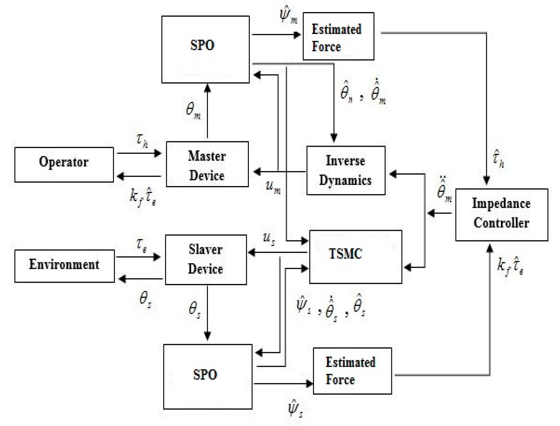
4. Bilateral Tele-Operation Control between Leader and Follower

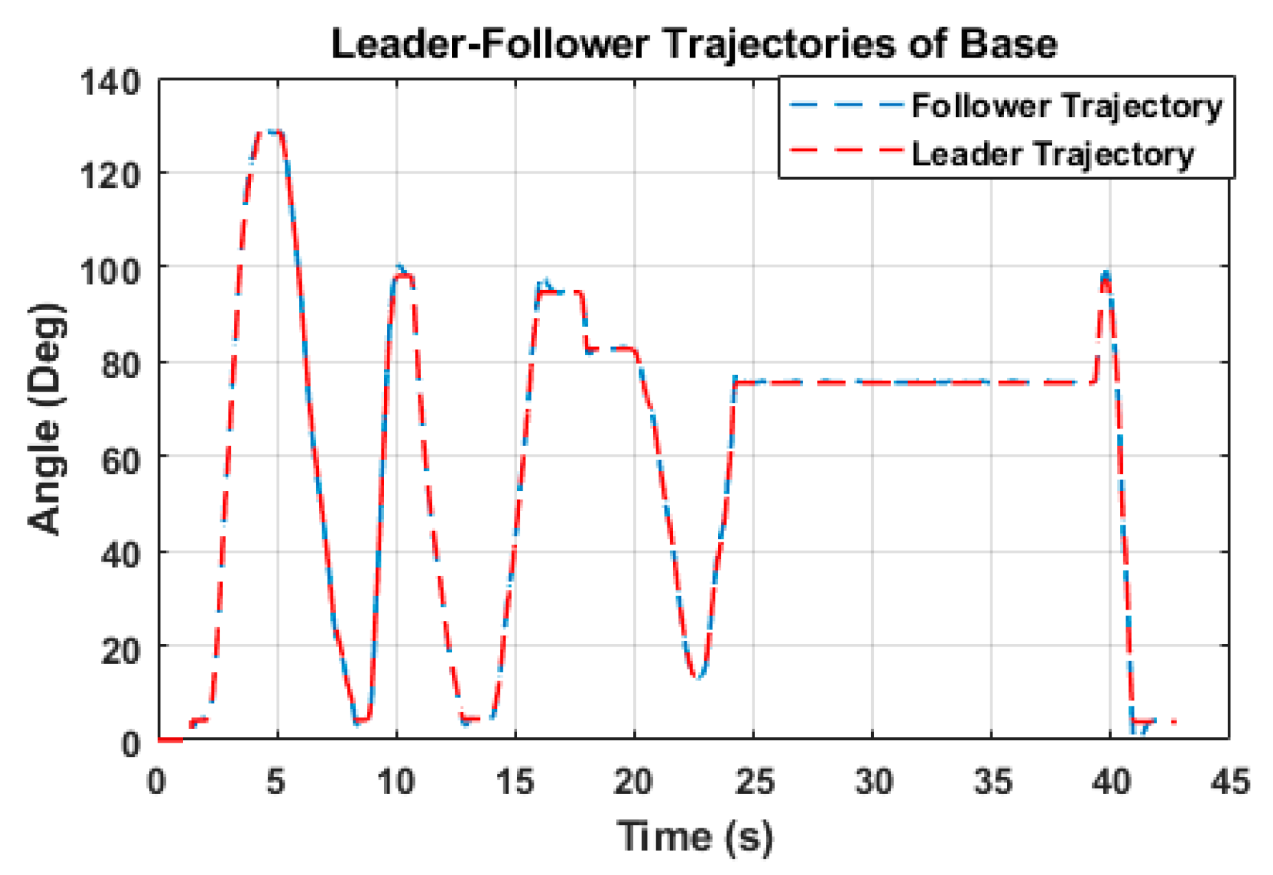
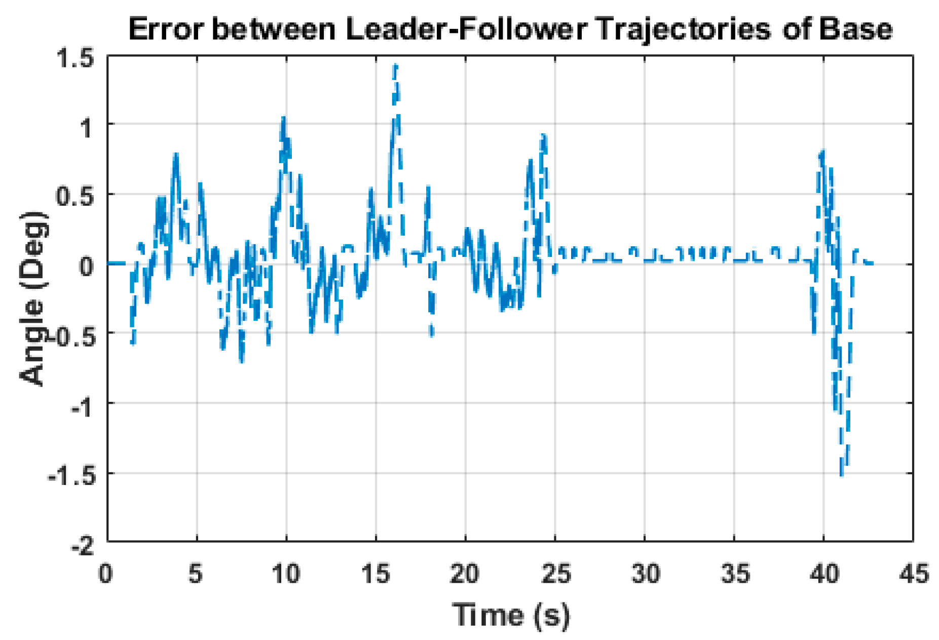
4.1. Bilateral Tele-Operation Control

First of all, the safety procedures were followed that ensured that the robotic actuators and end effectors did not pose a threat to the user or the surroundings. The system is a mixture of hydraulics and electronics, therefore, accidental spills of hydraulic fluids or electrocution due to electric wires were prevented. Consequently, the computers running client and server routines were powered-up. Here, in the context of the leader–follower configuration, the client refers to the follower while the server refers to leader. The client routine is executed after starting the server routine. The graphical user interface-based software was made using Microsoft Visual Studio in the Windows environment. The client robot attempts to connect with the server robot by utilizing the known parameters of IP address and port number. The server routine is waiting for approaching requests for establishing connection. Only after validating a connection request from the client robotic system does the server side authorize the connection. The leader robot requests the client identity, followed by sending a puzzle to the client. The client uses the established methodology of reversing the bits of the question and replies to the server in order to verify its identity. The status bar on the software turns green when the connection is successful, while it turns red if the connection failed. To ensure safety, the amplifiers are initially powered down (in case they were already powered up). After the successful link creation, the amplifiers are powered up again. This routine can be observed manually by using the “SWITCH ON” and “SWITCH OFF” buttons from the software. The operator presses the Read button on the leader computer followed by pressing the Read button on the follower computer. The leader software reads the data from encoders that provide the position information that is used to calculate the essential variables shown in the system equations. These variables are critical for tele-actuation and feedback. The validity of these variables is tested by making sure their values fall within the allowed range. Only the valid variable values are transferred to the follower computer. The orientation information of all axes is also sent to the follower using the TCP network socket. We used a TCP type network socket for reliable data transfer. Both of the leader and follower receive and transfer the data using their network sockets. The follower routine translates the variables into actuation commands according to the leader’s information. Upon the follower’s actuation, the software running on the follower computer reads the sensor value to compute the reaction force observed by the follower robot. This force calculation is performed by using a SMCSPO controller implemented in the software. Using the novel algorithm, the position and perturbation are projected and communicated to the leader computer using the already working network sockets. The communication can be continued flawlessly and without any delays for extended durations. The efficacy of the system was tested as the follower followed/tracked the leader positions. The block diagram for the complete system is shown in Figure 2. When a connection is broken due to any interruption at any side, the connection partner gets a notification for connection termination. This makes sure the amplifiers are powered down in case of any problems.

4.2. Bilateral Control

The bilateral control strategy is defined in such a way that the user (human operator) can give a trajectory to the leader and follower device can follow the trajectory of leader. The user can also feel the reaction force when the follower device interacts with the object. Leader and follower dynamics equation can be expressed as follow.

$$J_m{\ddot{\theta }}_m+B_m{\dot{\theta }}_m=u_m+{\tau }_h$$

(36)

$$J_s{\ddot{\theta }}_s+B_s{\dot{\theta }}_s=u_s-{\tau }_e$$

(37)

where $u$ describes the control input and $J$ signifies inertia. The structure of the bilateral control is demonstrated in Figure 3.

The leader device control input is described as follows:

$$u_m=(B_m-\frac{J_m}{J_d}{B}_d){\dot{\widehat{\theta }}}_m+(\frac{J_m}{J_d}-1){\widehat{\tau }}_h-\frac{J_m}{J_d}(k_f{\widehat{\tau }}_e+K{\widehat{\theta }}_m)$$

(38)

where $u_m$, ${\dot{\widehat{\theta }}}_m$, and ${\widehat{\theta }}_m$ are control input, estimated speed profile, and estimated position profile for the leader device, respectively, and ${\widehat{\tau }}_h$ is the estimated torque for the operator.

The user (human operator) gives instructions to the leader, and the follower manipulator follows those instructions. The controller for the follower device is considered through the TSMCSPO structure. The estimated sliding function is derived as,

$${\widehat{s}}_j={\dot{\widehat{e}}}_j+{\beta }_{j1}{\left|{\widehat{e}}_j\right|}^{r}sign\left(\widehat{e}\right)$$

(39)

where ${\widehat{e}}_j={\widehat{x}}_{1j}-x_{1dj}$ defines errors in tracking of the leader–follower device, ${\beta }_{j1}>0$ is constant. The new control for the follower device ${\overline{u}}_s$ is chosen such that it fulfills the criterion $\dot{\widehat{s}}\widehat{s}<0$. The dynamical equation for $\dot{\widehat{s}}$ is defined as,

$${\dot{\widehat{s}}}_j=-{\Gamma }_j{R}_{\max j}\left(k_{1j}/{\epsilon }_{0j}\right)sign({\widehat{s}}_j)-{\eta }_{3j}{\left|s_j\right|}^{r}sign({\widehat{s}}_j)$$

(40)

${\overline{u}}_s$ is chosen when ${\widehat{x}}_{2j}-\left(k_{1j}/{\epsilon }_{0j}\right){\tilde{x}}_{1j}-{\dot{x}}_{1dj}\ne 0,\widehat{e}\ne 0$

$${\overline{u}}_s=\frac{1}{{\alpha }_{3j}}\left\{\begin{array}{l}-{\Gamma }_j{R}_{\max j}\left(k_{1j}/{\epsilon }_{0j}\right)sign({\widehat{s}}_j)-{\eta }_{3j}{\left|s_j\right|}^{r}sign(\widehat{s})+\\ \left[k_{2j}/{\epsilon }_{0j}-{\left(k_{1j}/{\epsilon }_{0j}\right)}^2\right]{\tilde{x}}_{1j}-{\widehat{\Psi }}_j-\\ {\beta }_{j}r{\left|{\widehat{e}}_j\right|}^{r-1}\left({\dot{\widehat{x}}}_s-\left(k_{1j}/{\epsilon }_{0j}\right){\tilde{x}}_{1j}-{\dot{\widehat{x}}}_m\right)\\ +J_d^{-1}\left(B_d{\dot{\widehat{x}}}_m+K_d{\widehat{x}}_m-{\widehat{\tau }}_h+k_f{\widehat{\tau }}_e\right)\end{array}\right\}$$

(41)

If ${\widehat{x}}_{2j}-\left(k_{1j}/{\epsilon }_{0j}\right){\tilde{x}}_{1j}-{\dot{x}}_{1dj}\ne 0,\widehat{e}=0$

$${\overline{u}}_s=\frac{1}{{\alpha }_{3j}}\left\{\begin{array}{l}-{\Gamma }_j{R}_{\max j}\left(k_{1j}/{\epsilon }_{0j}\right)sign({\widehat{s}}_j)-{\eta }_{3j}{\left|s_j\right|}^{r}sign(\widehat{s})+\\ \left[k_{2j}/{\epsilon }_{0j}-{\left(k_{1j}/{\epsilon }_{0j}\right)}^2\right]{\tilde{x}}_{1j}+-{\widehat{\Psi }}_j-\\ {\beta }_{j}r{|\Delta |}^{r-1}\left({\dot{\widehat{x}}}_s-\left(k_{1j}/{\epsilon }_{0j}\right){\tilde{x}}_{1j}-{\dot{\widehat{x}}}_m\right)+\\ J_d^{-1}\left(B_d{\dot{\widehat{x}}}_m+K_d{\widehat{x}}_m-{\widehat{\tau }}_h+k_f{\widehat{\tau }}_e\right)\end{array}\right\}$$

(42)

If ${\widehat{x}}_{2j}-\left(k_{1j}/{\epsilon }_{0j}\right){\tilde{x}}_{1j}-{\dot{x}}_{1dj}=0$

$${\overline{u}}_s=\frac{1}{{\alpha }_{3j}}\left\{\begin{array}{l}-{\Gamma }_j{R}_{\max j}\left(k_{1j}/{\epsilon }_{0j}\right)sign({\widehat{s}}_j)-{\eta }_{3j}{\left|s_j\right|}^{r}sign(\widehat{s})+\\ \left[k_{2j}/{\epsilon }_{0j}-{\left(k_{1j}/{\epsilon }_{0j}\right)}^2\right]{\tilde{x}}_{1j}+\\ J_d^{-1}\left(B_d{\dot{\widehat{x}}}_m+K_d{\widehat{x}}_m-{\widehat{\tau }}_h+k_f{\widehat{\tau }}_e\right)-{\widehat{\Psi }}_j\end{array}\right\}$$

(43)

Thus, the follower manipulator control input can be determined through the expression,

$$u_s=J_s{\overline{u}}_s+B_s{\dot{\widehat{\theta }}}_s$$

(44)

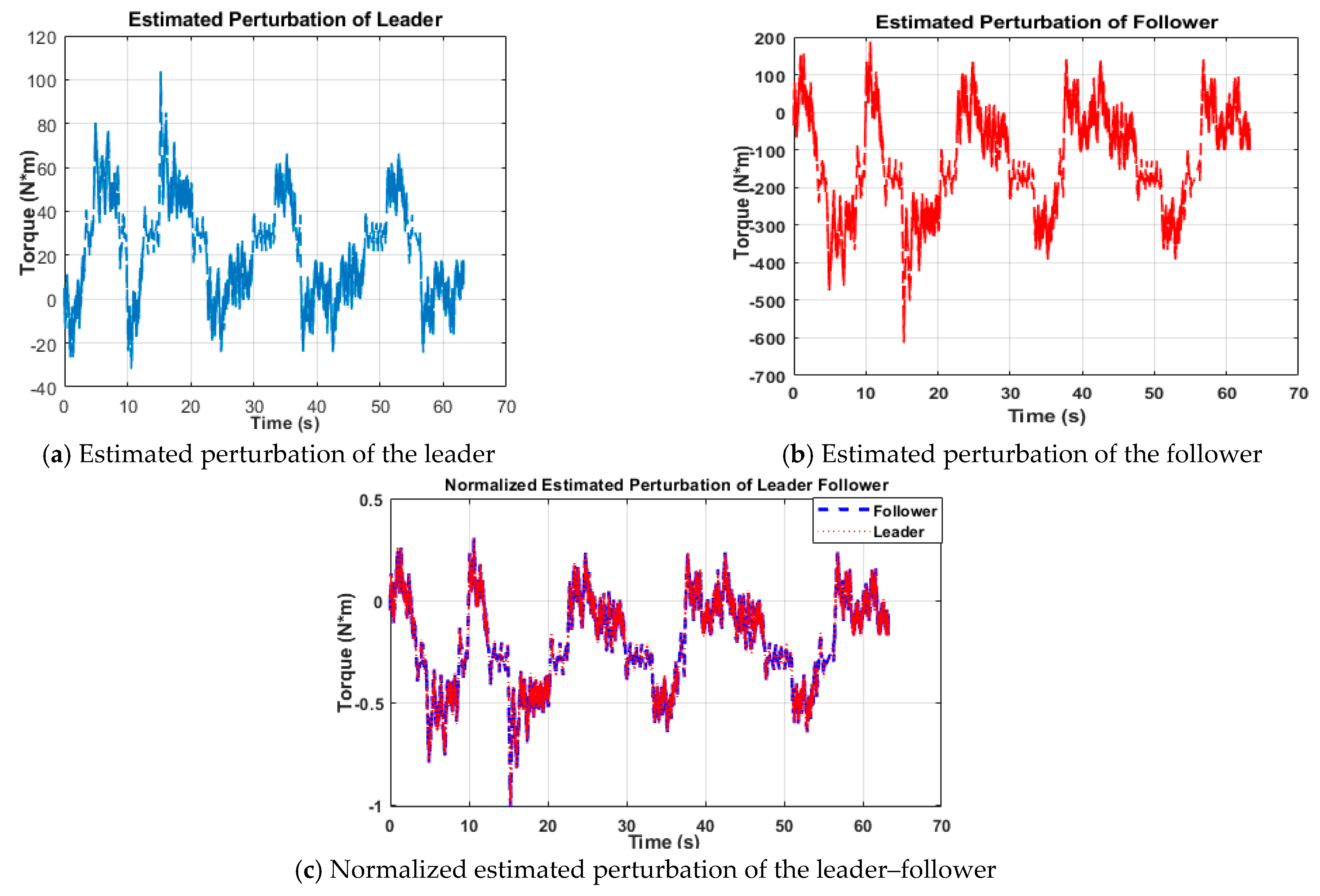
4.3. Estimation of Reaction Force Using a Sliding Perturbation Observer (SPO)

The perturbation can be estimated with the SPO and be based upon the purpose of the reaction-force. The estimation of perturbation is done through Equations (2) and (3) that define the dynamical representation of the three-DOF manipulator. This helps to calculate reaction force. Likewise, the estimation of the perturbation of 2nd link and end effector is,

$${\widehat{\psi }}_{s1}=-\frac{1}{J_{s1}}({\widehat{\tau }}_{e1})-\frac{1}{J_{s1}}(0.5M_{s1}{L}_{1}g\sin {\theta }_1)-(\frac{\Delta J_{s1}}{J_{s1}}){\ddot{\theta }}_1-\frac{1}{J_{s1}}(\Delta B_{s1}+{\beta }_1){\dot{\theta }}_1$$

(45)

$$\begin{array}{l}{\widehat{\psi }}_{s2}=-\frac{1}{J_{s2}}({\widehat{\tau }}_{e2})-\frac{1}{J_{s2}}(M_{s2}{L}_{2}g\cos {\theta }_2)-(\frac{\Delta J_{s2}}{J_{s2}}){\ddot{\theta }}_1\\ -\frac{1}{J_{s2}}(\Delta B_{s2}{\dot{\theta }}_2)-\frac{1}{J_{s2}}({\beta }_2\dot{x})-\frac{1}{J_{s2}}(\lambda )\end{array}$$

(46)

The calculation of reaction force by estimation of perturbation can be determined through Equations (46) and (47) as,

$${\widehat{\tau }}_{e1}=J_{s1}{\widehat{\psi }}_{s1}+0.5M_{s1}{L}_{1}g\sin {\theta }_1+\Delta J_{s1}{\ddot{\theta }}_1+(\Delta B_{s1}+{\beta }_1){\dot{\theta }}_1$$

(47)

$${\widehat{\tau }}_{e2}=J_{s2}{\widehat{\psi }}_{s2}+M_{s2}{L}_{2}g\cos {\theta }_2+\Delta J_{s2}{\ddot{\theta }}_1+\Delta B_{s2}{\dot{\theta }}_2+{\beta }_2\dot{x}+\lambda$$

(48)

where ${\widehat{\tau }}_{e1}$,${\widehat{\tau }}_{e2}$ are the estimated reaction-torques while connected to joint-1 or joint-2 and the environment, respectively, and $\Delta$ operator is the uncertainty parameter. The uncertainties could be considered as null if the values of the parameters are well estimated, i.e., fewer errors.

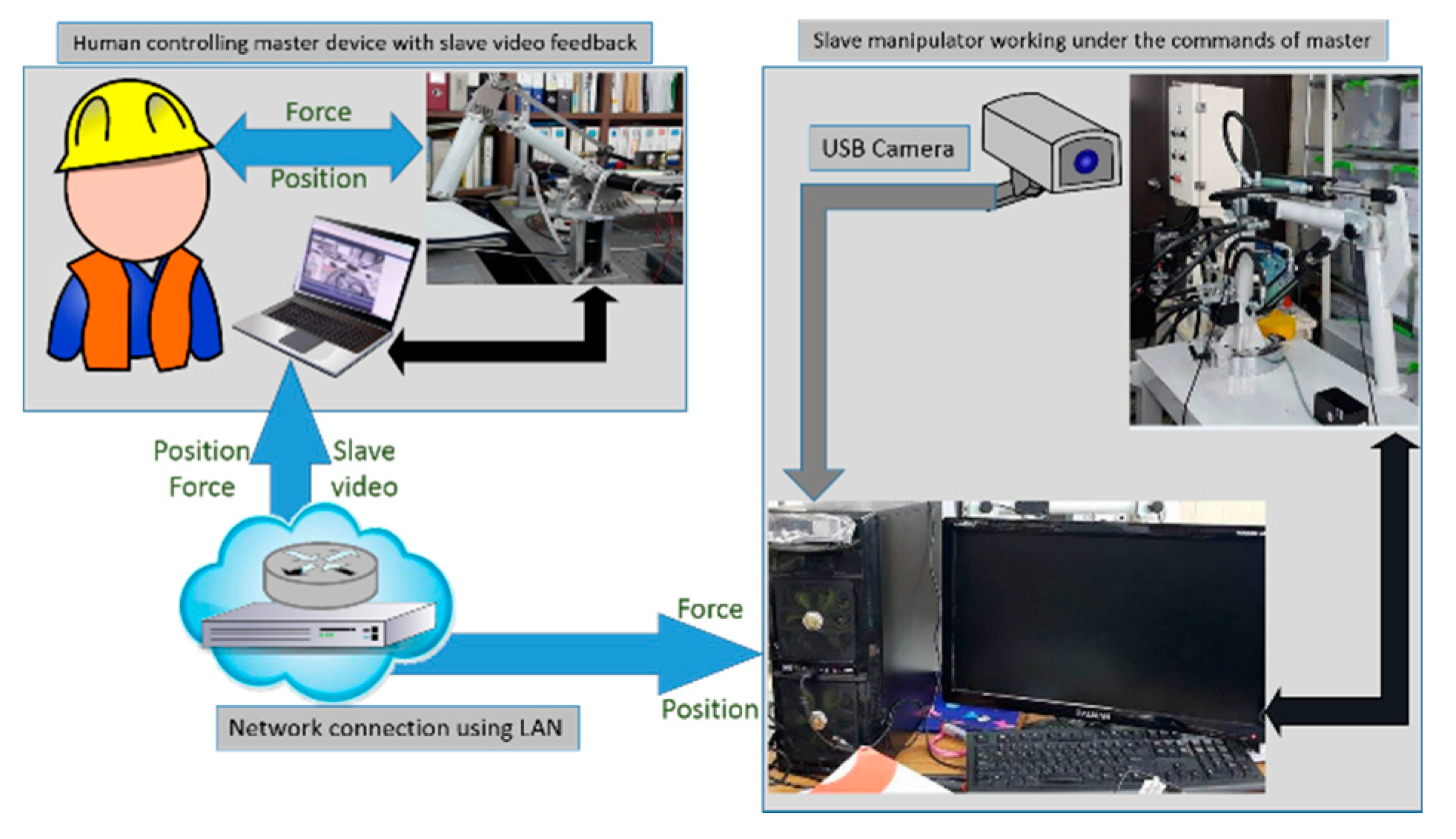
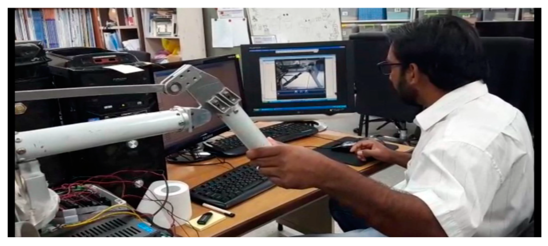
5. Internet-Based Experimental Setup

The leader device was placed on the 8th floor while the follower was place in the basement of the same building, and both the leader and follower manipulators had three links. Link-1 in both the leader and the follower manipulators connects to the base of the corresponding systems. The follower device in our system is a hydraulic manipulator that consists of a servo-motor and two cylinders. The follower device in our system is a hydraulic manipulator that comprises a servo motor and two cylinders. The purpose of the hydraulic cylinder is to actuate link number 2 and the end effector. Additionally, the servo motor is in place to control the base of our manipulator.

The control input of TSMCSPO can be calculated accordingly,

$$\overline{u}=\frac{1}{{\alpha }_{3j}}\left\{\begin{array}{l}-{\Gamma }_j{R}_{\max j}\left(k_{1j}/{\epsilon }_{0j}\right)sign({\widehat{s}}_j)-{\eta }_{3j}{\left|s_j\right|}^{r}sign(\widehat{s})+\\ \left[k_{2j}/{\epsilon }_{0j}-{\left(k_{1j}/{\epsilon }_{0j}\right)}^2\right]{\tilde{x}}_{1j}+{\ddot{x}}_{1dj}-{\widehat{\Psi }}_j-\\ {\beta }_{j}r{|\Delta |}^{r-1}\left({\widehat{x}}_{2j}-\left(k_{1j}/{\epsilon }_{0j}\right){\tilde{x}}_{1j}-{\dot{x}}_{1dj}\right)\end{array}\right\}$$

(49)

We used the three-DOF hydraulic manipulator to carry our extensive experimentation. The reaction forces were generated at the end effector and the second link. The reaction forces were estimated with the aforementioned TSMCSPO algorithm. The human operator present in the basement (leader) location produced the trajectory for leader manipulator, which was then tracked by the follower manipulator on the 8th floor of the building. A visual display on a personal computer was provided to the human operator at the leader device location. The schemes of the SMC controlled the trajectory of the follower manipulator as per leader manipulator command. Figure 4 represents the leader device and the GUI for visual feedback.

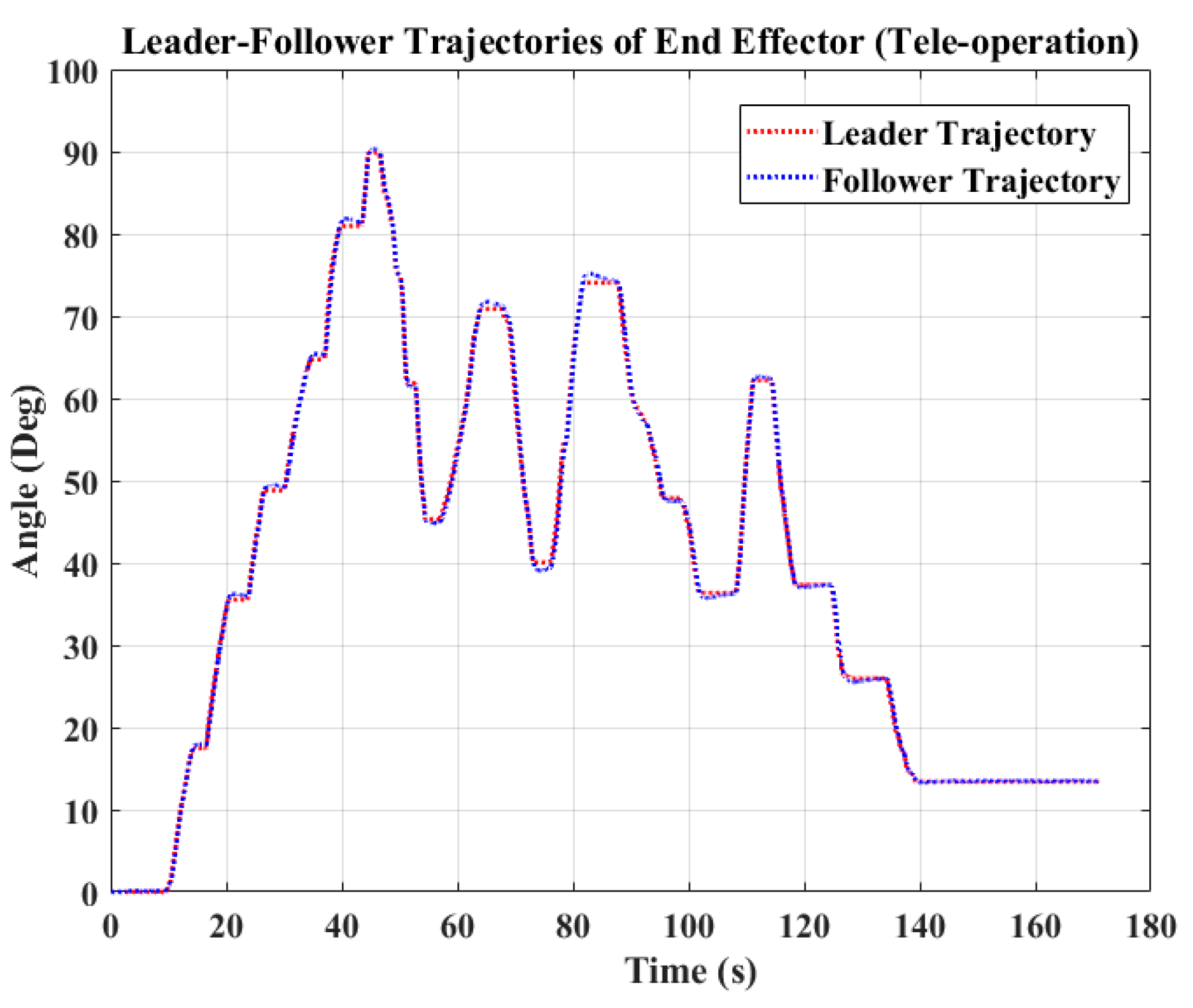
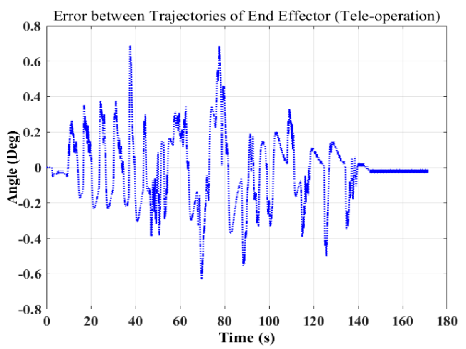
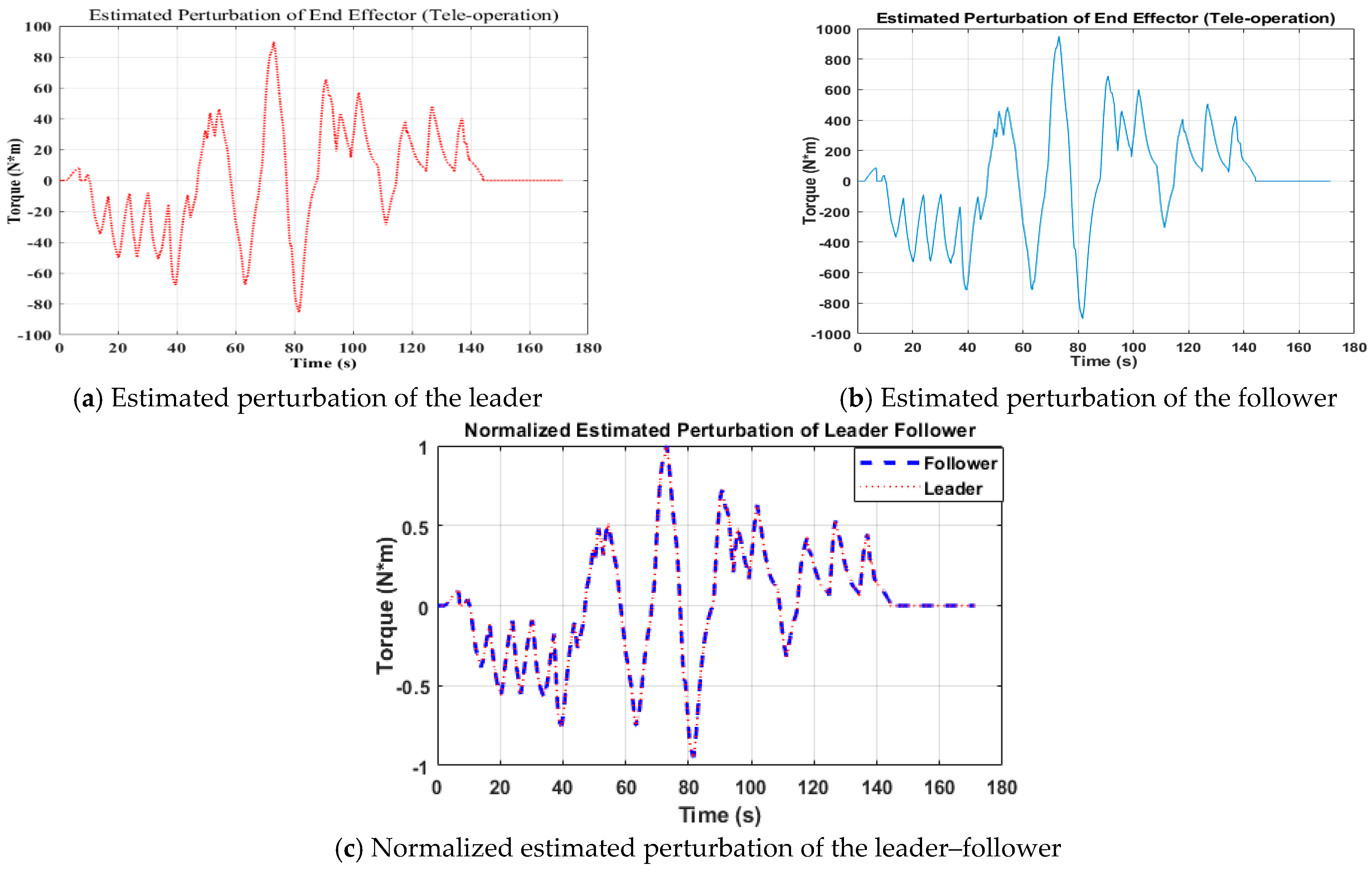
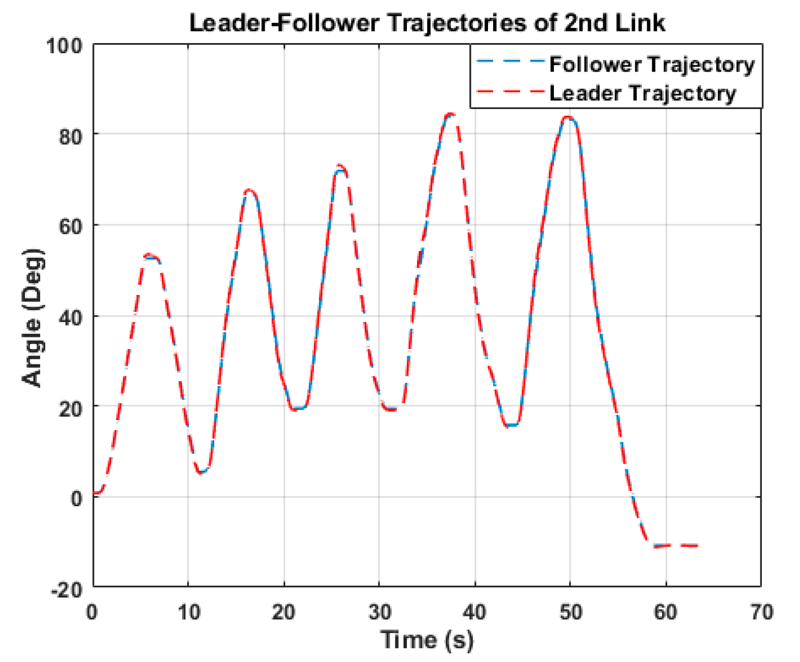
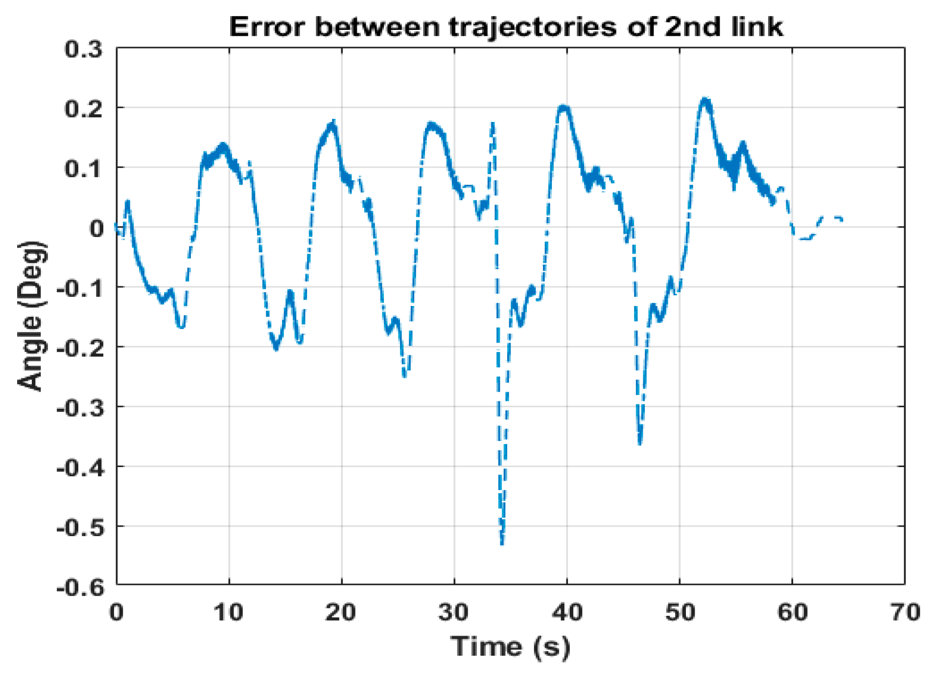
6. Experimental Results

Table 1. Design parameters.

Parameters	Values
$K_{}$ (End effector)	25
$K_{}$ (2nd Link)	250
$K_{}$ (Base)	8
$k_1$	39
$k_2$	507
${\epsilon }_0$	1
$c$	13
$e$	1
${\alpha }_3$ (End effector)	4.08
${\alpha }_3$ (2nd Link)	10
${\alpha }_3$ (Base)	2.58

showed the parameter values of the TSMCSPO that were used in the experimental work.

The tele-operated bilateral control strategy using the TSMCSPO was verified by performing many experiments under different circumstances. The scenarios of the experiment included the following: (1) Tele-operated bilateral control of the leader and follower position tracking of the end effector; (2) Leader–follower perturbation estimation of the end effector; (3) Tele-operated bilateral control of the leader and follower position tracking of the second link; (4) Leader–follower perturbation estimation of the second link; (5) Tele-operated bilateral control of the leader and follower position tracking of the base; (6) Follower perturbation estimation of the base; (7) Tele-operated bilateral control of the leader and follower position tracking of the end effector when in contact with the environment; and (8) Leader-follower perturbation estimation of end effector when in contact with the environment. These experimentations were accomplished in an actual system where a human operator gave trajectories to the leader and the follower device followed according to the command evaluated by the TSMCSPO. From the first experiment, the results of the tele-operated bilateral control for position tracking of end effector are shown in Figure 5. The position of the leader device is shown with the blue dotted line while the position of the follower device is shown with the red dotted line of the base, end effector, and second link. The results of Figure 5 show that the follower device tracked the commands of the human operator, which were given to the leader device, with little inconsistency. A flawless tracking of the follower shows the competence of the proposed structure (TSMCSPO). It is also perceived from the results the that maximum value of the trajectories of the leader–follower was attained at 90 degrees at 45.4 s of the end effector. The end effector can move between 0 and 90 degrees in space.

The inaccuracy between the leader–follower trajectories of the end effector are demonstrated in Figure 6. The extreme value of the error observed between the leader–follower trajectories was 0.6865 degrees at 77.57 s. It is also perceived from the results that 0.32 degrees is the average error between the leader–follower trajectories.

Figure 7a,b shows the results of the leader–follower estimated perturbation for the end effector separately. The uppermost values of the estimated perturbation are at 73.11 s for the leader and follower manipulators. The values of the leader and follower are 90.04 N∙m and 950.57 N∙m separately.

The result of the estimated perturbation for the follower device shows a higher value as compared to that of the leader device. The reason for the superiority of the follower manipulator is the hydraulic manipulator. The dynamical value of the follower is 303.26 which is higher that that of the leader device value, i.e., 1.35135. The estimated perturbations of the leader–follower profiles are the same but with opposite directions. Leader–follower normalized values of the estimated perturbation lie in the range of [−1,1]. The calculation of normalized values is completed as follows:

$$P_{norm}(Leader)=\frac{a_i-\min (a)}{\max (a)-\min (a)}, i=1,\dots ,N$$

(50)

$$P_{norm}(Follower)=\frac{a_i-\max (a)}{\max (a)-\min (a)}, i=1,\dots ,N$$

(51)

where $a_i$ is the ith perturbation value. The result of the normalized estimated perturbation of leader–follower manipulator for the end effector is represented in Figure 7c. The result of the normalized value for leader is shown with a red-dotted line, while the blue-dashed line represents the results of follower manipulator.

The results in Figure 8 show that the follower device of second link tracked the command of the human operator, which was given to the leader device with the least inconsistency. It is also perceived from the results that the maximum value of the trajectories of the leader–follower attained 84.4 degrees at 37.42 s of second link. The second link can move between 0 and 90 degrees in space.

The inaccuracy between the leader–follower trajectories of the second link are demonstrated in Figure 9. The extreme value of the error observed between the leader–follower trajectories was 0.5373 degrees at 34.25 s. It is also perceived from the results that 0.23 degrees was the average error between the leader–follower trajectories.

Figure 10a,b indicates the results of the leader–follower estimated perturbations for the end effector separately. The uppermost values of the estimated perturbation were at 15.26 s for the leader and follower manipulators. The values of the leader and follower are 103.3 N∙m and 613.1 N∙m, respectively. The results of the normalized estimated perturbation of the leader–follower manipulator for the end effector are represented in Figure 10c. The results of the normalized value for the leader is shown in a red-dotted line the while blue-dashed line represents the results of the follower manipulator.

Figure 11 show that the follower device of the base tracked the command of the human operator, which was given to the leader device with the least inconsistency. The second link can move from 0 to 360 degrees in space. It is also perceived from the results that the maximum value of the trajectories of the leader–follower attained 128.5 degrees at 4.51 s of the base.

An inconsistency in tracking of the base is presented in Figure 12. The extreme value of the error observed between the leader–follower trajectories was 1.528 degrees at 41.26 s. It is also perceived from the results that 0.09 degrees was the average error between the leader–follower trajectories. Figure 13 indicates the results of the follower’s estimated perturbation for the base. The uppermost value of the estimated perturbation was at 15.7 s for the follower manipulator. The value of the follower manipulator was 163.6 N∙m.

Figure 14 shows that the follower device of the end effector tracked the command of the human operator, which was given to the leader device when the follower manipulator was in contact with the environment. It is evident the follower’s end effector follows the leader’s trajectory, but when it was in contact with the environment there was a difference between both trajectories. It is also perceived from the results that the maximum value of the trajectories of the leader–follower attained 89.53 degrees at 134.6 s of the base.

Figure 15a,b indicates the results of the leader–follower estimated perturbations for the end effector separately. The uppermost values of the estimated perturbation were at 111.6 s for the leader and follower manipulators. The values of the leader and follower were 113.74 N∙m and 2012.3 N∙m, respectively. The results of the normalized estimated perturbation of leader–follower manipulator for the end effector is represented in Figure 15c. The result of normalized value for the leader is shown in a blue-dashed line while the red-dotted line represents the results of the follower manipulator.

As we can see from the figures, the estimated perturbation is increased when follower end effector touches the environment at 100 s and human operator can also feel the reaction force. After some time, the operator pulls back the end effector from contact with the environment. The estimated perturbation is increased to reach the maximum value and then there is drop in estimated perturbation when the operator stops pushing.

7. Conclusions

This study proposed a method that can calculate the reaction force from estimated perturbations by the SPO. Perturbation includes not only an external force but also elements that affect the reaction force estimation, such as model parameter errors of the mass and viscous friction, coulomb friction, interactive forces of manipulators, etc. Therefore, this new algorithm can reduce the uncertain effects in the estimated perturbation value and can calculate the pure reaction force. In addition, a tele-operated bilateral controller was designed based on the TSMCSPO for robust control of the follower. From the experimental results, it was confirmed that the proposed tele-operated bilateral controller has guaranteed good tracking performance of position and estimated reaction force in real time.

In this research, we have shown that the tele-operated bilateral control could be used in the dismantling of a nuclear power plant where human access is not possible. The results of this study can be applied in the dismantling of nuclear power plants, but they are not limited to that application as several other applications require leader–follower systems where human access is limited. These applications include those in hazardous areas with radiation from material with long half-lives, for example, uranium transportation in its active form, the disposal of explosive materials or handling of explosive/radioactive materials, and remote cutting in nuclear plant dismantling, etc. In our proposed scheme, we used a local area network that is also available in nuclear power plants. Therefore, we can avoid control performance degradation by utilizing a local area network. In the future, work will be done on a global network in which the time-delay will be a major issue. In GAN, the delay of latency almost remains constant throughout the communication, but the jitter’s delay varies over time. In the future, modern techniques will need to tackle the delay issues related to GAN.

References

1. Locatelli, G.; Mancini, M. A Framework for the Selection of the Right Nuclear Power Plant. Int. J. Prod. Res. 2011, 50, 4753–4766. [Google Scholar] [CrossRef]
2. Kamada, N.; Saito, O.; Endo, S.; Kimura, A.; Shizuma, K. Radiation doses among residents living 37 km northwest of the Fukushima Dai-ichi Nuclear Power Plant. J. Environ. Radioact. 2012, 110, 84–89. [Google Scholar] [CrossRef]
3. Khan, H.; Abbasi, S.J.; Kallu, K.D.; Lee, M.C. Robust control design of 6-DOF robot for nuclear power plant dismantling. In Proceedings of the 2019 International Conference on Robotics and Automation in Industry (ICRAI), Rawalpindi, Pakistan, 21–22 October 2019; pp. 1–7. [Google Scholar]
4. Tsitsimpelis, I.; Taylor, C.J.; Lennox, B.; Joyce, M.J. A review of ground-based robotic systems for the characterization of nuclear environments. Prog. Nucl. Energy 2019, 111, 109–124. [Google Scholar] [CrossRef]
5. Mallion, A.; Wilson, C.; Smith, R.; Ferguson, G.; Roberts, R.; Hilton, P. LaserSnake2: An Innovative Approach to Nuclear Decommissioning-17080; WM Symposia, Inc.: Tempe, AZ, USA, 2017. [Google Scholar]
6. Freschi, C.; Ferrari, V.; Melfi, F.; Ferrari, M.; Mosca, F.; Cuschieri, A. Technical review of the da Vinci surgical telemanipulator. Int. J. Med Robot. Comput. Assist. Surg. 2013, 9, 396–406. [Google Scholar] [CrossRef] [PubMed]
7. Baser, O.; Konukseven, E.I. Utilization of motor current based torque feedback to improve the transparency of haptic interfaces. Mech. Mach. Theory 2012, 52, 78–93. [Google Scholar] [CrossRef]
8. Lovasz, E.-C.; Mărgineanu, D.T.; Ciupe, V.; Maniu, I.; Gruescu, C.M.; Zăbavă, E.S.; Stan, S.D. Design and control solutions for haptic elbow exoskeleton module used in space telerobotics. Mech. Mach. Theory 2017, 107, 384–398. [Google Scholar] [CrossRef]
9. Ozaki, H.; Mohri, A.; Takata, M. On the force feedback control of a manipulator with a compliant wrist force sensor. Mech. Mach. Theory 1983, 18, 57–62. [Google Scholar] [CrossRef]
10. Yip, M.C.; Yuen, S.G.; Howe, R.D. A Robust Uniaxial Force Sensor for Minimally Invasive Surgery. IEEE Trans. Biomed. Eng. 2010, 57, 1008–1011. [Google Scholar] [CrossRef] [PubMed] [Green Version]
11. Puangmali, P.; Liu, H.; Seneviratne, L.D.; Dasgupta, P.; Althoefer, K. Miniature 3-axis distal force sensor for minimally invasive surgical palpation. IEEE ASME Trans. Mechatron. 2011, 17, 646–656. [Google Scholar] [CrossRef]
12. Kang, J.S.; Lee, M.C.; Yoon, S.M. Bilateral control based rupture protection method in surgical robot using improved leader device. Int. J. Control Autom. Syst. 2016, 14, 1073–1080. [Google Scholar] [CrossRef]
13. Peñaloza-Mejía, O.; Márquez-Martínez, L.A.; Alvarez-Gallegos, J.; Alvarez, J. Leader-follower teleoperation of underactuated mechanical systems with communication delays. Int. J. Control Autom. Syst. 2017, 15, 827–836. [Google Scholar] [CrossRef]
14. Murakami, T.; Yu, F.; Ohnishi, K. Torque sensorless control in multidegree-of-freedom manipulator. IEEE Trans. Ind. Electron. 1993, 40, 259–265. [Google Scholar] [CrossRef]
15. Katsura, S.; Matsumoto, Y.; Ohnishi, K. Modeling of force sensing and validation of disturbance observer for force control. IEEE Trans. Ind. Electron. 2004, 54, 530–538. [Google Scholar] [CrossRef]
16. Tadano, K.; Kawashima, K. Development of 4-DOFs forceps with force sensing using pneumatic servo system. In Proceedings of the 2006 IEEE International Conference on Robotics and Automation, ICRA 2006, Orlando, FL, USA, 15–19 May 2006; pp. 2250–2255. [Google Scholar]
17. Smith, A.C.; Mobasser, F.; Hashtrudi-Zaad, K. Neural-network-based contact force observers for haptic applications. IEEE Trans. Robot. 2006, 22, 1163–1175. [Google Scholar] [CrossRef]
18. Mitsantisuk, C.; Ohishi, K.; Katsura, S. Estimation of action/reaction forces for the bilateral control using Kalman filter. IEEE Trans. Ind. Electron. 2011, 59, 4383–4393. [Google Scholar] [CrossRef]
19. Aviles, A.I.; Alsaleh, S.M.; Hahn, J.K.; Casals, A. Towards Retrieving Force Feedback in Robotic-Assisted Surgery: A Supervised Neuro-Recurrent-Vision Approach. IEEE Trans. Haptics 2017, 10, 431–443. [Google Scholar] [CrossRef] [Green Version]
20. Kallu, K.D.; Jie, W.; Lee, M.C. Sensorless reaction force estimation of the end effector of a dual-arm robot manipulator using sliding mode control with a sliding perturbation observer. Int. J. Control Autom. Syst. 2018, 16, 1367–1378. [Google Scholar] [CrossRef]
21. Kallu, K.D.; Abbasi, S.J.; Lee, M.C. Estimation force of leader-follower for the end effector of hydraulic servo system using SMCSPO. In Proceedings of the 2017 17th International Conference on Control, Automation and Systems (ICCAS), Jeju, Korea, 18–21 October 2017; pp. 1665–1668. [Google Scholar]
22. Dad, K.; Jie, W.; Abbasi, S.J.; Lee, M.C. Reaction force estimation and bilateral control of leader follower manipulation using a robust controller. In Proceedings of the 2017 10th International Conference on Human System Interactions (HSI), Ulsan, Korea, 17–19 July 2017; pp. 178–181. [Google Scholar]
23. Kallu, K.D.; Abbasi, S.J.; Lee, M.C. Bilateral control of hydraulic servo system for end-effector of leader-follower manipulators. In Proceedings of the 2017 14th International Conference on Ubiquitous Robots and Ambient Intelligence (URAI), Miyazaki, Japan, 19–22 January 2017; pp. 284–287. [Google Scholar]
24. Jie, W.; Dad, K.; Lee, M.C. A reaction force estimation method of end effector of two-link manipulator using SMCSPO. In Proceedings of the 2016 13th International Conference on Ubiquitous Robots and Ambient Intelligence (URAI), Xi’an, China, 19–22 August 2016; pp. 869–872. [Google Scholar]
25. Jie, W.; Dad, K.; Lee, M.-C. SMCSPO based force estimation for a hydraulic cylinder. In Proceedings of the 2017 17th International Conference on Control, Automation and Systems (ICCAS), Jeju, Korea, 18–21 October 2017; pp. 1422–1425. [Google Scholar]
26. Kallu, K.D.; Abbasi, S.J.; Yaqub, M.A.; Lee, M.C. Tele-operated bilateral control of hydraulic servo system using estimated reaction force of end effector by SMCSPO. In Proceedings of the 2018 15th International Conference on Ubiquitous Robots (UR), Honolulu, HI, USA, 26–30 June 2018; pp. 57–62. [Google Scholar]
27. Martinez, D.I.; De Rubio, J.J.; Vargas, T.M.; Garcia, V.; Ochoa, G.; Balcazar, R.; Cruz, D.R.; Aguilar, A.; Novoa, J.F.; Aguilar-Ibanez, C. Stabilization of Robots With a Regulator Containing the Sigmoid Mapping. IEEE Access 2020, 8, 89479–89488. [Google Scholar] [CrossRef]
28. Escobedo-Alva, J.O.; Garcia-Estrada, E.C.; Paramo-Carranza, L.A.; Meda-Campana, J.A.; Tapia-Herrera, R. Theoretical application of a hybrid observer on altitude tracking of quadrotor losing GPS signal. IEEE Access 2018, 6, 76900–76908. [Google Scholar] [CrossRef]
29. Aguilar-Ibanez, C.; Suarez-Castanon, M.S. A Trajectory Planning Based Controller to Regulate an Uncertain 3D Overhead Crane System. Int. J. Appl. Math. Comput. Sci. 2019, 29, 693–702. [Google Scholar] [CrossRef] [Green Version]
30. García-Sánchez, J.R.; Tavera-Mosqueda, S.; Silva-Ortigoza, R.; Hernández-Guzmán, V.M.; Sandoval-Gutiérrez, J.; Marcelino-Aranda, M.; Taud, H.; Marciano-Melchor, M. Robust Switched Tracking Control for Wheeled Mobile Robots Considering the Actuators and Drivers. Sensors 2018, 18, 4316. [Google Scholar] [CrossRef] [Green Version]
31. Amini, H.; Dabbagh, V.; Rezaei, S.; Zareinejad, M.; Mardi, N.; Sarhan, A.A. Robust control-based linear bilateral teleoperation system without force sensor. J. Braz. Soc. Mech. Sci. Eng. 2015, 37, 579–587. [Google Scholar] [CrossRef]
32. Cao, C.; Wang, F.; Cao, Q.; Sun, H.; Xu, W.; Cui, M. Neural network–based terminal sliding mode applied to position/force adaptive control for constrained robotic manipulators. Adv. Mech. Eng. 2018, 10, 1687814018781288. [Google Scholar] [CrossRef] [Green Version]
33. Dinh, T.X.; Tran, T.; Anh, T.H.V.; Ahn, K.K. Disturbance Observer Based Finite Time Trajectory Tracking Control for a 3 DOF Hydraulic Manipulator Including Actuator Dynamics. IEEE Access 2018, 6, 36798–36809. [Google Scholar] [CrossRef]
34. Rahmani, M.; Rahman, M.H. Novel robust control of a 7-DOF exoskeleton robot. PLoS ONE 2018, 13, e0203440. [Google Scholar] [CrossRef] [PubMed]
35. Vo, A.T.; Kang, H.-J. An Adaptive Terminal Sliding Mode Control for Robot Manipulators with Non-Singular Terminal Sliding Surface Variables. IEEE Access 2019, 7, 8701–8712. [Google Scholar] [CrossRef]
36. Han, S.I.; Lee, J. Finite-time sliding surface constrained control for a robot manipulator with an unknown deadzone and disturbance. ISA Trans. 2016, 65, 307–318. [Google Scholar] [CrossRef]
37. Wang, J.; Lee, M.C.; Kallu, K.D.; Abbasi, S.J.; Ahn, S. Trajectory Tracking Control of a Hydraulic System Using TSMCSPO based on Sliding Perturbation Observer. Appl. Sci. 2019, 9, 1455. [Google Scholar] [CrossRef] [Green Version]
38. Elmali, H.; Olgac, N. Sliding mode control with perturbation estimation (SMCPE): A new approach. Int. J. Control 1992, 56, 923–941. [Google Scholar] [CrossRef]
39. Moura, J.T.; Elmali, H.; Olgac, N. Sliding Mode Control with Sliding Perturbation Observer. J. Dyn. Syst. Meas. Control. 1997, 119, 657–665. [Google Scholar] [CrossRef]
40. Slotine, J.-J.; Sastry, S.S. Tracking control of non-linear systems using sliding surfaces, with application to robot manipulators. Int. J. Control 1983, 38, 465–492. [Google Scholar] [CrossRef] [Green Version]
Figure 1. Schematic diagram of articulated hydraulic manipulator.
Remotesensing 13 01648 g001
Figure 2. Schematic diagram of tele-operation.
Remotesensing 13 01648 g002
Figure 3. Structure of the bilateral control.
Remotesensing 13 01648 g003
Figure 4. Video feedback.
Remotesensing 13 01648 g004
Figure 5. Position tracking of the leader–follower for the end effector using the TSMCSPO.
Remotesensing 13 01648 g005
Figure 6. Position tracking error of the end effector.
Remotesensing 13 01648 g006
Figure 7. Estimated perturbation of the leader–follower for the end effector.
Remotesensing 13 01648 g007
Figure 8. Position tracking of the leader–follower for the second link using the TSMCSPO.
Remotesensing 13 01648 g008
Figure 9. Position tracking error of the second link.
Remotesensing 13 01648 g009
Figure 10. Estimated perturbation of the leader–follower for the second link.
Remotesensing 13 01648 g010
Figure 11. Position tracking of the leader–follower for the base using the TSMCSPO.
Remotesensing 13 01648 g011
Figure 12. Position tracking error of base.
Remotesensing 13 01648 g012
Figure 13. Base estimated perturbation.
Remotesensing 13 01648 g013
Figure 14. Position tracking of the leader–follower for the end effector with the environment.
Remotesensing 13 01648 g014
Figure 15. Estimated perturbation of the leader–follower with the environment.
Remotesensing 13 01648 g015