Article

Monitoring of Urban Sprawl and Densification Processes in Western Germany in the Light of SDG Indicator 11.3.1 Based on an Automated Retrospective Classification Approach

1
Geomatics Group, Institute of Geography, Faculty of Geosciences, Ruhr-University Bochum, 44870 Bochum, Germany
2
Leibniz Centre for Agricultural Landscape Research (ZALF), 15374 Müncheberg, Germany
3
nextPlace, Detmold School of Architecture, Interior Design and Urban Planning, TH Ostwestfalen-Lippe, 32756 Detmold, Germany
4
Center for Remote Sensing of Land Surfaces (ZFL), University of Bonn, 53113 Bonn, Germany
5
German Remote Sensing Data Center (DFD), German Aerospace Center (DLR), Münchener Straße 20, 82234 Weßling, Germany
6
Department of Remote Sensing, University of Würzburg, Oswald-Külpe-Weg 86, 97074 Würzburg, Germany
*
Author to whom correspondence should be addressed.
Submission received: 1 March 2021 / Revised: 13 April 2021 / Accepted: 20 April 2021 / Published: 27 April 2021
(This article belongs to the Special Issue Understanding Urban Systems Using Remote Sensing)

Abstract

:
By 2050, two-third of the world’s population will live in cities. In this study, we develop a framework for analyzing urban growth-related imperviousness in North Rhine-Westphalia (NRW) from the 1980s to date using Landsat data. For the baseline 2017-time step, official geodata was extracted to generate labelled data for ten classes, including three classes representing low, middle, and high level of imperviousness. We used the output of the 2017 classification and information based on radiometric bi-temporal change detection for retrospective classification. Besides spectral bands, we calculated several indices and various temporal composites, which were used as an input for Random Forest classification. The results provide information on three imperviousness classes with accuracies exceeding 75%. According to our results, the imperviousness areas grew continuously from 1985 to 2017, with a high imperviousness area growth of more than 167,000 ha, comprising around 30% increase. The information on the expansion of urban areas was integrated with population dynamics data to estimate the progress towards SDG 11. With the intensity analysis and the integration of population data, the spatial heterogeneity of urban expansion and population growth was analysed, showing that the urban expansion rates considerably excelled population growth rates in some regions in NRW. The study highlights the applicability of earth observation data for accurately quantifying spatio-temporal urban dynamics for sustainable urbanization and targeted planning.

Graphical Abstract

1. Introduction

An urban sprawl that often results in the conversion of natural vegetation cover and the expansion of the spatial footprint of impervious surfaces is one of the most striking land-use changes. Urbanization, which is caused by economic development and continuous population growth, as well as changing lifestyles, and residential and retail uses within the urban fringes is one of the most important drivers of terrestrial change [1,2]. As the global trend of urbanization is expected to further increase the urban share of the world population from about 55 percent in 2018 to 68 percent by 2050 [3], understanding transformations of urban areas, and navigating those transformations towards more sustainable path-ways is of high societal relevance. Growing urbanization makes urban areas highly dynamic [4], thus, making the research on the detection of land-use patterns of great importance.
One of the critical components of rapid urbanization is the expansion of impervious surfaces. These areas, such as building rooftops, roads, parking areas, which comprise residential, industrial, or commercial land continuously take over large areas of natural and semi-natural land (e.g., grassland, forest and cropland area). The main part of urban areas, the area and dynamics of impervious surfaces can be used as an essential indicator for evaluating the degree of urban sprawl [2,5,6]. Therefore, the assessment of extent, spatial patterns, and dynamics of impervious surfaces [7] is crucial in further understanding the impacts on urban development, population distribution and density, social conditions, and fluctuating house prices.
Among the Sustainable Development Goals (SDGs) Goal 11 highlights the importance of “making cities inclusive, safe, resilient and sustainable.” The targets associated with this goal, namely target 11.3, focuses on the sustainable urbanization and improvement of opportunities for participatory, integrated and sustainable urban planning and management [8,9,10]. Specifically, the indicator SDG 11.3.1, defined as the ratio of the land consumption rate to the population growth rate, is used to describe the relationship between urban expansion and demographic change. A global study in 2011 shows that urban areas have grown more than three times as much as the urban population [11]; studies at national level showed a difference of three-to-five times [12]. Considering that the spatial and demographic changes in the urban areas are essential to understanding the progress towards sustainable growth, assessment of the linkages between urban expansion and demographic change can be beneficial for sustainable urbanization, as well as targeted planning, in order to effectively monitor land consumption growth [13].
In order to monitor progress towards SDG 11 and accompanying targets, such as SDG 11.3.1, there is a need for accurate and timely representation of different aspects of urban conditions, including land cover and land use (LC/LU) [14]. The assessment of urban change and expansion can deeply benefit from Earth Observation (EO). It is recognized as one of the main tools for urban monitoring as it provides continuous spatiotemporal data [15,16,17,18]. Based on Remote sensing (RS) images and derived metrics different methods for urban mapping have been developed [19,20], such as per-pixel sub-pixel (linear spectral unmixing) analysis, and data fusion with volunteered geographic information [18]. EO has the capacity to significantly supplement to demographic and other spatial data, at a large scale, at varying spatial resolution, and repeatedly over time [10,11], which can be used both in the SDG framework [6,12,13], and in general, for the development of urban development indicators [14,21]. These indicators often rely on medium or high-resolution satellite image-based classification using per-pixel, sub-pixel (based on vegetation-impervious surface-soil model), and object-based methods. Among these methods, sub-pixel information extraction, with different algorithms based on spectral mixture analysis, have been developed [5,6,22]. Nevertheless, these models tend to overestimate in regions with small impervious areas and underestimate in regions with large proportions, due to the similarity in spectral properties among vegetation, soil, and impervious surface materials [23].
Several methods have been described for satellite-based imperviousness change analysis, such as pre- and post-classification approaches. The multi-temporal stacked images are classified directly when using the pre-classification approach. Although it has been shown to be accurate for impervious surface mapping, it requires comprehensive reference data, including both land cover labels, and information on change type [2,24,25,26]. The post-classification analysis classifies each image individually, and information regarding the change is derived based on per-pixel comparison [27,28], nevertheless, the limited availability of multi-temporal retrospective reference data has been a challenge [29].
Several global products exist that map settlements, which were produced with the use of RS data, such as the Global Human Settlement Layer (GHSL) [30], the Global Urban Footprint (GUF) [31] and the World Settlement Footprint (WSF) [32]. These products have a high spatial resolution, abstract artificial land as built-up areas and urban footprints, and have global coverage. Furthermore, at a European level, Copernicus high-resolution layers provide several thematic layers, including the imperviousness level [33]. Although the data have high spatial resolution and relevant thematic context, it is only available for five-time steps (2006–2018), thus, limiting the analysis of densification processes to a smaller, recent time interval. Besides the limitation of different continental to global land cover products, with the limited coverage over time, available long-term products often lack thematic context and present data that support the analysis of single class (built-up areas/urban/settlement) changes [9]. Therefore, within-class densities and their dynamics are often not assessed.
Urbanization has been one of the most prominent change processes in Central Europe coupled with simultaneous sociodemographic changes [34,35]. Around 73% of the European population lives in cities, which is projected to reach 82% by 2050. The expansion of built-up areas was observed in most regions of Europe, even in areas where the population has declined [36]. In Germany, the land consumption and reallocation of natural and agricultural land to built-up and transportation-related areas exceeds 60 ha per day [24,37,38]. Although in recent years, artificial development in Germany has shown decrease, especially for diffuse residential sprawl, the area around industrial and commercial sites has increased significantly during 2006–2012, which was followed by decline in the period 2000–2006 [39]. Therefore, the need to monitor and accurately quantify these changes increases. In Germany, in general, but also in the German federal state of North Rhine-Westphalia (NRW), parallel development has been observed, with a distinct growth of settlements and transportation infrastructure. In the national sustainability strategy, presented in 2002, the 30-ha goal was introduced by the German government aimed at reducing Germany’s land consumption to a maximum of 30 ha per day until 2030 [4]. Although the daily land consumption has declined during the past years, it was still at 10 ha per day in NRW [40]. Furthermore there were changes applied to the cadastral data recording, which made the year-to-year comparison challenging. Alongside the introduction of ALKIS (Official Real Estate Cadaster Information System) as the official real estate cadaster information system, all German federal states have replaced their previous records. In NRW, the last cadastral authorities switched over in 2015. With the changes in some of the categories of cadastral system [41], the areas belonging to the category “urban” have not changed much in terms of quantity, but a lot in terms of location.
Based on this, the objectives of this study are; first, to implement an automated retrospective classification approach for observing land use and imperviousness dynamics during the last 30 years; second, to analyze the spatial trends of urban sprawl in NRW, and; third to assess the intensity of densification and population dynamics to support the monitoring of SDG indicator 11.3.1.

2. Study Area and Data

2.1. Study Area

The study area covers the German federal state of North-Rhine Westphalia (NRW) (Figure 1). It is the most densely populated state in Germany, counting 526 persons per km2 [42]. NRW has 396 municipalities, including 22 independent cities. Different LC/LU characterizes this area. Around half of the state area is covered by seminatural arable lands, and forests cover 20%. Built-up areas comprise around 20% of the area. The area includes the Rhine-Ruhr Metropolitan Area (RRMA) (Figure 1), which is the largest metropolitan region in Germany with over 10 million inhabitants [42], and which has the largest area of continuously high urban sprawl [36]. Although the population has decreased during the last decade in NRW, the population has grown from 1985 to 2017 by more than 7% [42]. Unlike the trends within the RRMA mentioned above, some areas, such as Cologne and Düsseldorf, which are the largest cities in NRW, had a continuous population increase. During the same period, the land area within NRW dedicated to settlement and transportation infrastructure increased [40]. Accordingly, the study area is heterogeneous and challenging when it comes to monitoring urban change dynamics, along with the highly urbanized areas, it comprises rather rural areas that are currently experiencing high urbanization rates.

2.2. Data

Due to the study’s long time-span, Landsat surface reflectance Level-2 data (https://espa.cr.usgs.gov/, last accessed on 24 April 2021) were selected as the primary source of data. We targeted at 5-year steps from 1985 and downloaded data for 1985, 1990, 1995, 2000, 2005, 2010, 2015, and 2017. Landsat sensors (TM, ETM+, OLI) provide advantages for urban growth monitoring and change detection, in terms of spatial resolution (30 m × 30 m), spectral characteristics (visible, near infrared, shortwave infrared, thermal infrared), and temporal coverage.
As the primary source of reference information, official geodata from the German Authoritative Topographic-Cartographic Information System (ATKIS) was extracted, in order to generate labeled data for 10 classes. For the classes water, coniferous, mixed, and deciduous forests, arable land, grassland, and open-pit mine samples were extracted from the Digital-base Landscape Model (BASIS-DLM) for 2017. In ATKIS DLM, the topographic features of the landscape are described by point, line, and shape in vector format with information describing residential area, traffic, vegetation, water, administrative area, and relief forms, with each category containing additional levels (e.g., different types of roads) [16]. ATKIS data are available since 1990, and the data are continuously updated. Unfortunately, it is not possible to reconstruct past time steps from the official release. Therefore, reference data exists only for 2017 in this study. In order to further interpret the change patterns in the study area, population data for administrative regions in NRW were extracted and analyzed [42].

3. Methods

The proposed method can be summarized in three major steps (Figure 2). The first step is data preparation and pre-processing of Landsat images. The second step is the baseline classification, implemented for the year 2017, which included the generation of labeled data for three imperviousness classes as well as the classification with a land-use map as an output. In the third step, we perform a per-pixel change detection analysis to detect pixels that are stable between two-time steps, and thus, can be used as an input for classification. This procedure was iterated for the years that preceded 2015, resulting in five change detection analysis. Detailed procedures of the approach are described below.

3.1. Data Processing

To overcome the impact of cloud and cloud shadow, we used the FMASK algorithm for Landsat cloud masking [43]. Images with more than 80% clouds were excluded from further analyses. Following the cloud mask, we calculated spectral indices, namely the Normalized Difference Vegetation Index (NDVI) [44,45] and the Normalized Difference Water Index (NDWI) [46], as well as Tasseled cap wetness, greenness and brightness (Table 1) [47]. We implemented a pixel-based compositing approach before the classification procedure and calculated temporal metrics [48,49,50,51] (e.g., 10th, 25th, 50th, 75th, 80th and 90th percentiles of annual time series, as well as a minima and maxima for both annual and growing season time series), which resulted in composites for each target year. We extracted eleven types of image features from each compositing result, including six surface reflectance (green, blue, red, NIR, SWIR1 and SWIR2) bands and the spectral indices (NDVI, NDWI, TC greenness, wetness, brightness). As there were differences in the coverage of cloud free pixels during different years, the imagery was reduced to the growing season (e.g., 1985, 2010). Therefore, the total number of input features that was used in a single year classification was 99. Since it was not possible to generate a gapless dataset for 1985 the imagery from 1986 was used as well. Due to the low quality of the composite in 1995, this timestep was excluded from further analysis.

3.2. Land Cover and Land Use Classification

To create the land-use maps for seven timesteps, the Random Forest (RF) [52] classifier was selected, as it is known to be robust for large-area land cover classification [53,54,55], and specifically useful with a large number of features [2]. For all classifications, the RF classifier was implemented with 500 trees and the square root of the total number of input variables as the number of variables to split at each node. The analysis was mainly carried out with R statistical software (randomForest package [56]) [57].
As one of the aims of the study was to estimate the changes with the differentiation of several imperviousness classes, an additional step was carried out for the generation of samples for the baseline year. First, regression was run based on ATKIS data. The data in ATKIS DLM, which represents residential areas, as well as roads were used. On a generated 30 m grid, the percentage of the cover of each grid cell with different built-up surfaces was estimated. Then RF regression was used to create a continuous layer at 30 m resolution showing the degree of imperviousness. Based on this layer, three classes of high, middle and low imperviousness samples were separated based on the percentage of the impervious area, corresponding to higher than 80%, 40–80% and less than 40% impervious surfaces per pixel. [22,58,59]. Similar classification schemes can be observed in other products, such as Corine Land cover, where continuous urban fabric class corresponds to areas with more than 80% imperviousness [60]. This approach has been shown to be suitable for deriving consistent classification results in urban areas with the required high precision. Furthermore, it identifies which regions experience scattered, diffusive, and dispersed urban growth. Combined with the thematic information, representing the other classes, RF classifier was run for 2017 with the use of 20,000 samples. The classes represent both environmentally and socio-economically important classes that can also capture the changes during the time span of the study. These classes include vegetated areas, such as forests, croplands and grasslands, as well as impervious areas. We separated water class to capture water bodies in the study area. As NRW includes highly industrial areas with formerly intensive coal mining, we included a separate class for open pit mine, in order to reduce the misclassification of these areas with urban classes.
Following the generation of accurate output for the baseline year, the Iteratively Reweighted Multivariate Alteration Detection (IR-MAD) was used [61,62], in order to derive the areas with no change, which are the basis for the extraction of reference samples for the classification of the preceding timestep. The IR-MAD transformation identifies suitable invariant pixels for radiometric normalization with a multivariate change detection algorithm [41] that iteratively increases the weight of non-change observations, and thereby, enhances the discrimination of substantial spectral changes between images from different time periods [63,64]. For our analysis, only the median composites of spectral bands and indices (in total 11 bands) were used in the change detection procedure, and a threshold of 0.25 was chosen for the chi-square image based on the IR-MAD algorithm to extract the unchanged area.
Finally, based on baseline classification and change detection, we applied a stepwise classification framework to former years by selecting new training samples using spectral information from unchanged pixels. Due to the changes between the timesteps and the subsequent decrease of the number of unchanged pixels, the number of samples decreased with each timestep. We assessed the accuracy of the final maps based on confusion matrices [65]. For the classification reference, we split the data randomly proportionally for training and validation. From these, we derived overall accuracy (OA), as well as producer’s (PA) and user’s (UA) accuracy.
The baseline map of 2017 was compared to the two available products at national level [66,67].

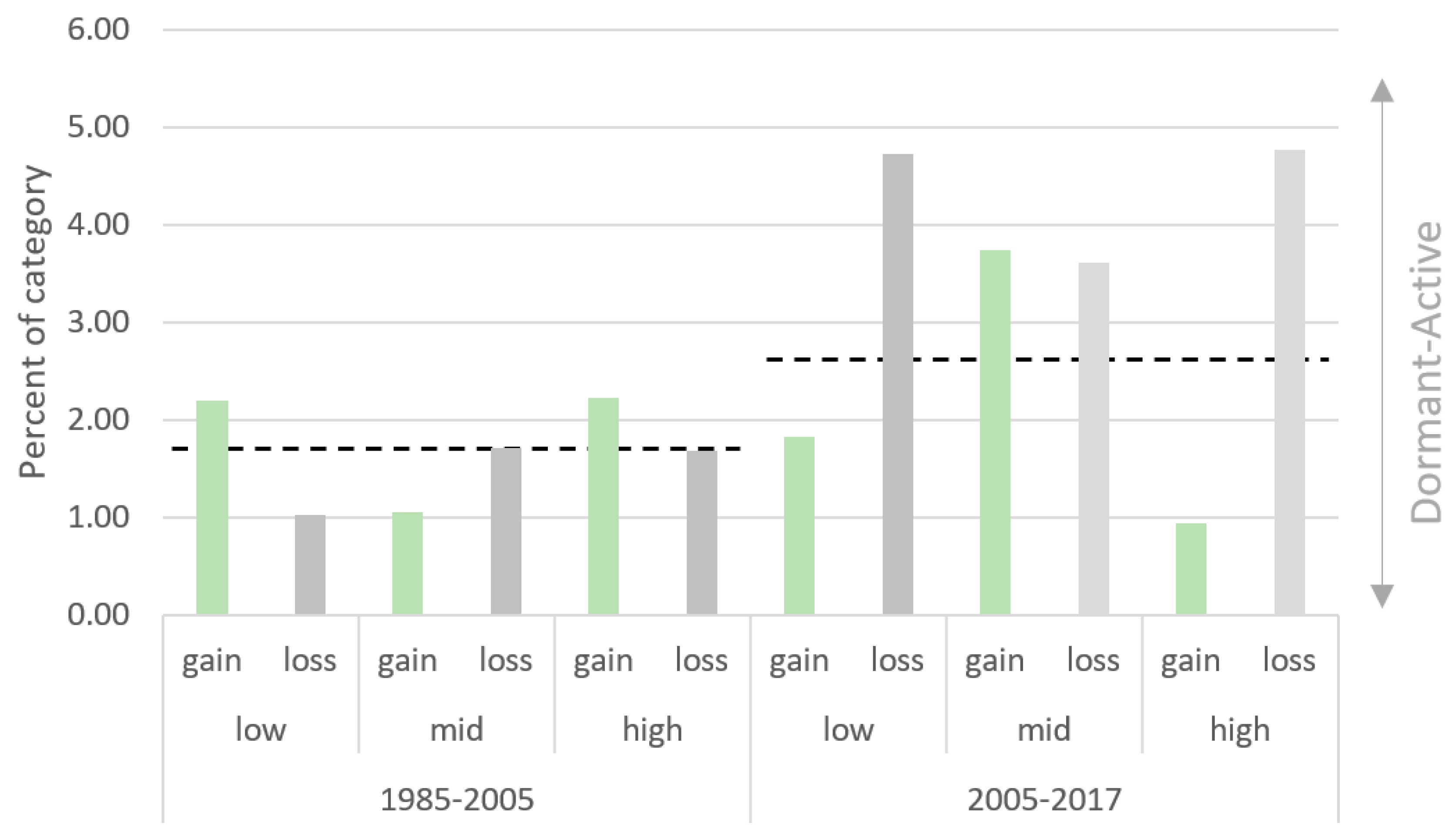
3.3. Intensity Analysis and Comparison with Population Data

To further understand the underlying processes of land-use change and urban growth and to evaluate whether the growth was sustainable, intensity analysis was applied. In general, the intensity analysis evaluates the predicted uniform rate of change compared to the observed rate of change among categories [68,69], characterizing the process of land use change. It also evaluates the land use change by setting the stability. Although the stable land use conversion may not always result in sustainable development, it can still be an indicator and basis for it [70].
Furthermore, the population data at a district level were used to compare the rates of urban growth and population change and calculate the ratio of land consumption rate (LCR) to population growth rate (PGR). It is based on the ratio of Land Consumption Rate and Population Growth Rate (LCRPGR) (Equations (1)–(3)) [8,51,71],
LCRPGR = LCR / PGR
LCR = LN ( Urb ( t + N ) / Urb t ) y
PGR = LN ( Pop ( t + N ) / Pop t ) y
where Urbt and Urb(t+N) is the areal extent of the land consumed at the initial reference year t and at the final year t + N; Popt and Pop(t+N) input the total population of the spatial unit at the initial reference year and at the final reference year, y is the number of years between t and t + N.

4. Results and Discussion

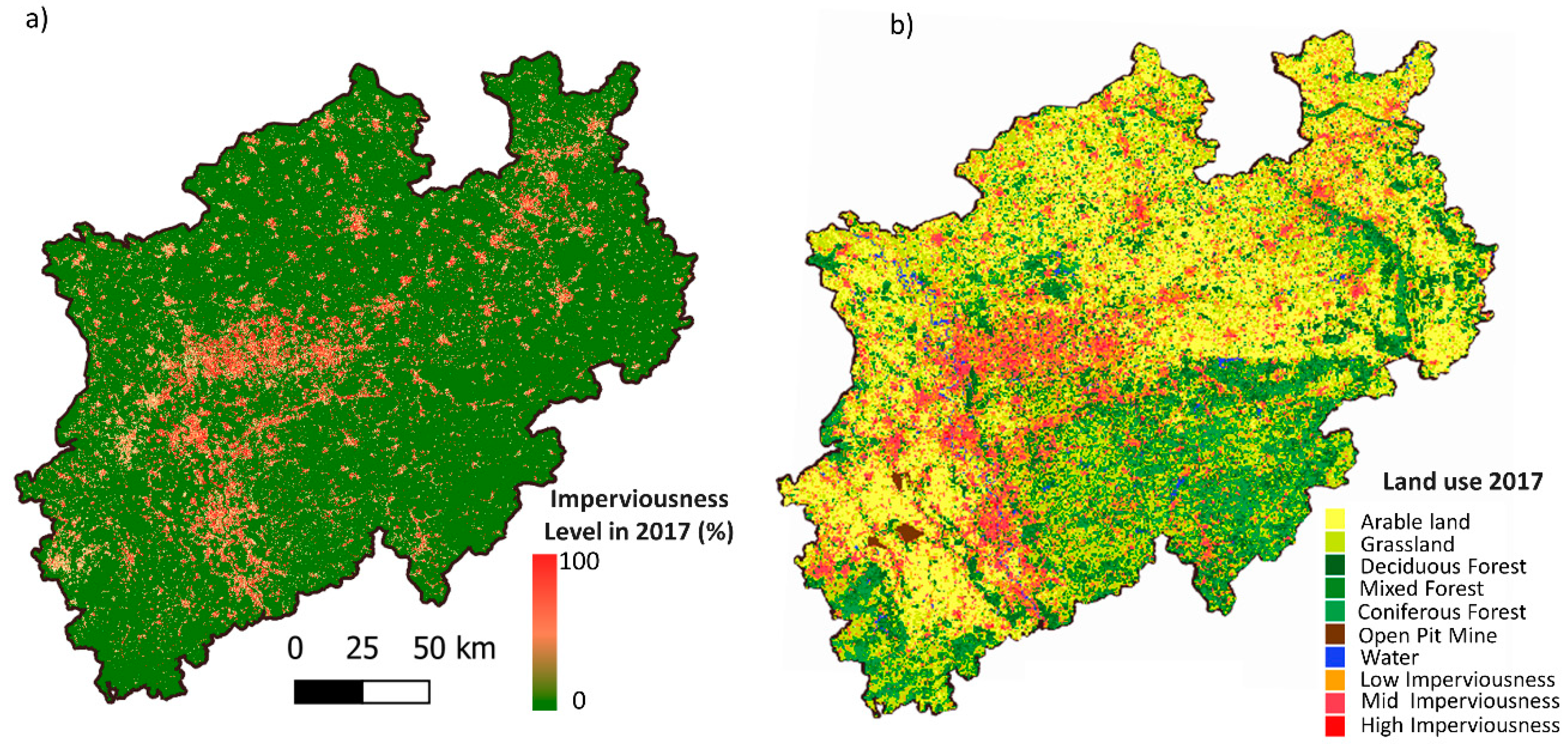
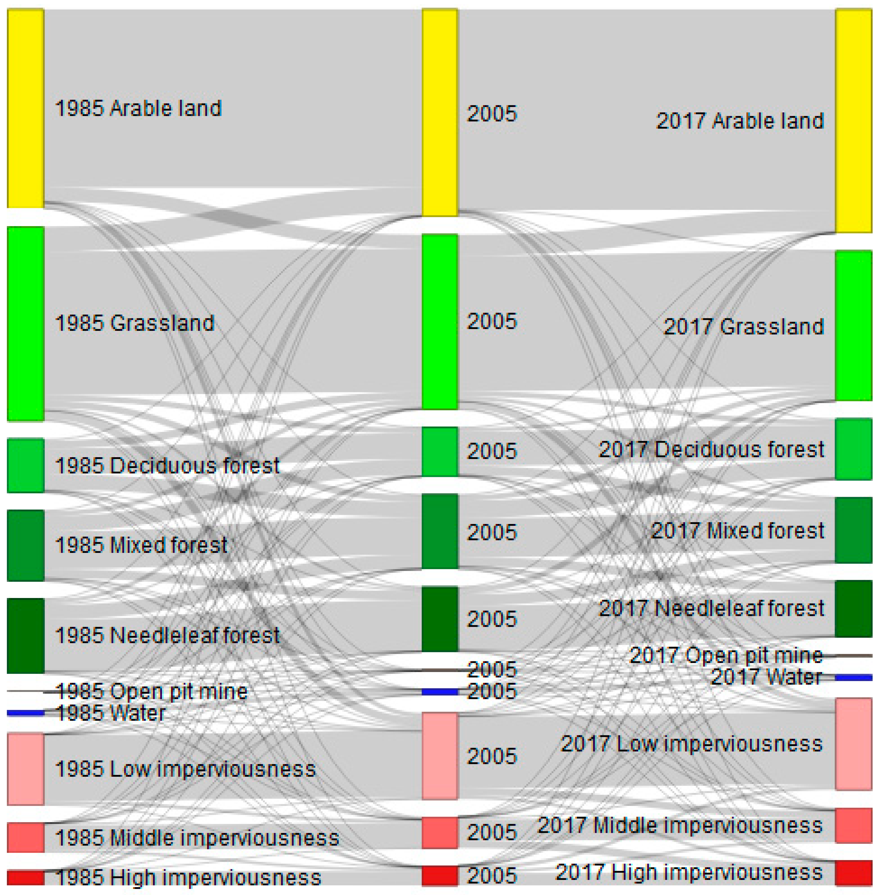
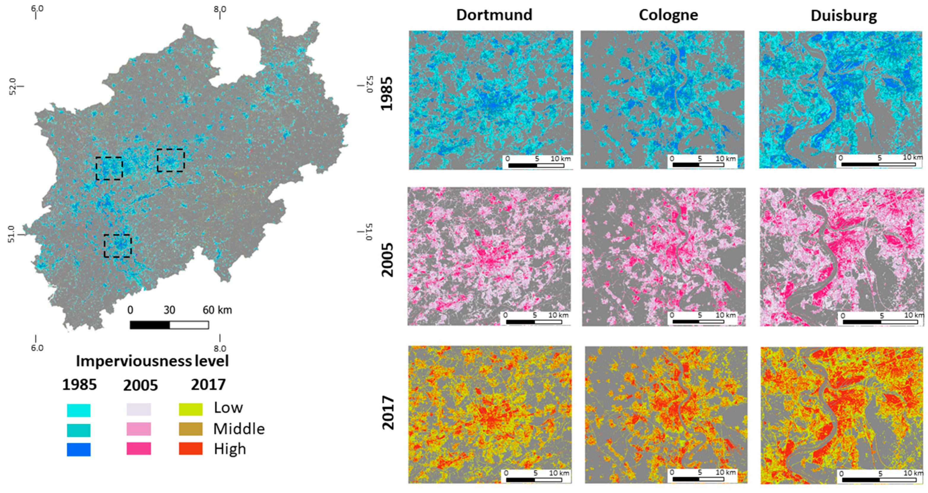
4.1. Land-Use Classification and Changes between 1985–2017

The classified maps differentiated between ten classes: Arable land, grassland, deciduous forest, coniferous forest, mixed forest, water, open-pit mines as well as low, medium, and high levels of imperviousness. The baseline classification of 2017 as well as the levels of imperviousness based on RF regression are shown in Figure 3. The resulting maps had acceptable quality, exceeding 75% of overall accuracy. Table 2 presents the OA, UA and PA for all time steps and UA and PA for the three impervious classes as the main target of the study in particular. The baseline map of 2017 was compared to the two available products at national level [66,67]. The maps had high agreement, especially for the classes of high- and mid-levels of imperviousness with the interim land cover product for class build up [66]. Whereas, all imperviousness classes had high agreement with class artificial land in the case of a second product [67].
We observed an accuracy decrease for the retrospective classification. Several factors can cause this accuracy decrease. First, due to the change detection, the number of unchanged pixels that can be used for training and validation decreases over the years. In the case of our study the total number of reference data decreased by 50% from 2017 to 1985. At the same time, we observe a large drop in accuracies for the time step of 1990, which has the biggest interval for change detection. Furthermore, the resolution of Landsat (30 m), which is higher than the size of many urban objects, can be the cause of mixed pixels and result in misclassifications [15]. We observed this issue, especially for low imperviousness levels, which exhibited lower PA and UA.
In contrast, the high impervious class was the most accurately classified class, with accuracies exceeding 80%. Another reason for the drop in accuracy can be the reduced data availability before the launch of Landsat-7 in 1999. Among the input variables, NDVI and NDWI, TC brightness minima and maxima, as well as green, red, NIR, and SWIR median and 90th percentile were among the essential input bands for classification. The combination of these metrics provided information on three imperviousness classes, helping to minimize misclassifications by minimizing seasonal effects and changes.
For 32 years, urban expansion resulted in large-scale increases in other land-use types transforming into a different level of imperviousness. The transitions of land-use are shown in Figure 4. The year 2005 was selected as a middle timestep, as it followed the implementation of the national sustainability strategy in 2002. It can be seen that arable land, forests, and grassland are the primary land resources for urban expansion. Transitions cause the increase in the low imperviousness class from arable land, grassland, and small changes in the forest classes. Simultaneously, a high level of dynamics can be observed between the three imperviousness classes, indicating a transition from low to middle and high level of imperviousness. The analysis of the maps shows that impervious surfaces comprised about 552,464 ha in 1985. Three decades later, impervious surfaces increased by more than 167,000 ha in 2017. The multiyear classification can contribute to quantification of the changes in areas where time series of reference data is not available. Specifically, according to the study of the Federal Institute for Research on Building, Urban Affairs and Spatial Development concluded that an accurate monitoring of land consumption during the conversion period from ALK/ALB to ALKIS, i.e., before and after 2016, is not less than difficult [72]. Three alternative databases were compared but none of them fulfilled the criteria of a possible replacement. ATKIS and LBM-DE (Digital land cover model for Germany) data are often outdated. Accordingly, the suggested approach provides insights on land consumption in NRW with a high resolution and temporal consistence. This makes the data of high value for researchers and the official statistical offices.
Because the degree and dynamics of imperviousness can be used as critical indicators for assessing the sustainability of land-use changes, we analyzed the intensity level of the changes (Table 3). The interval level of intensity shows the size and speed of change across different time intervals. The category level of the intensity analysis gives information about which land use category is relatively dormant or active during a particular time interval. During our study period, the 2005–2017 interval was fast compared to uniform growth, while the earlier 1985–2005 interval was slower than uniform growth.
At the category change intensity of grassland, water, forests, as well as low and high imperviousness exhibited greater than the average intensity during 1985–2005, indicating active change. The changing intensity of arable land was less than the average intensity, indicating rather dormant change. Between 2005 and 2017, open-pit mine and the middle imperviousness class exhibited greater than average change intensity. The rate at which other land use categories are converted to imperviousness is higher than the transition rate of imperviousness classes to other land use categories.
Based on the results of our intensity analysis, between 1985 and 2005 the high and middle imperviousness classes were targeted from the low imperviousness class. In the case of 2005–2017, transitions from low to high impervious level were largely avoided.
The gain intensity of impervious areas (Figure 5) in the first interval was higher than the annual uniform intensity of 1.71 for the low and the high imperviousness classes, thus making them an active land use category. During this period, other classes, such as arable land or open-pit mine were dormant, with gain intensity lower than uniform. For the second interval, compared to the uniform change rate of 2.72, the middle imperviousness level was an active class. Coupled with the analysis at a community level (Figure 6), these metrics can reveal the patterns of urban change. When considering the net urban growth, the more rural eastern region in NRW had the highest relative gains during the last 30 years (Figure 6).

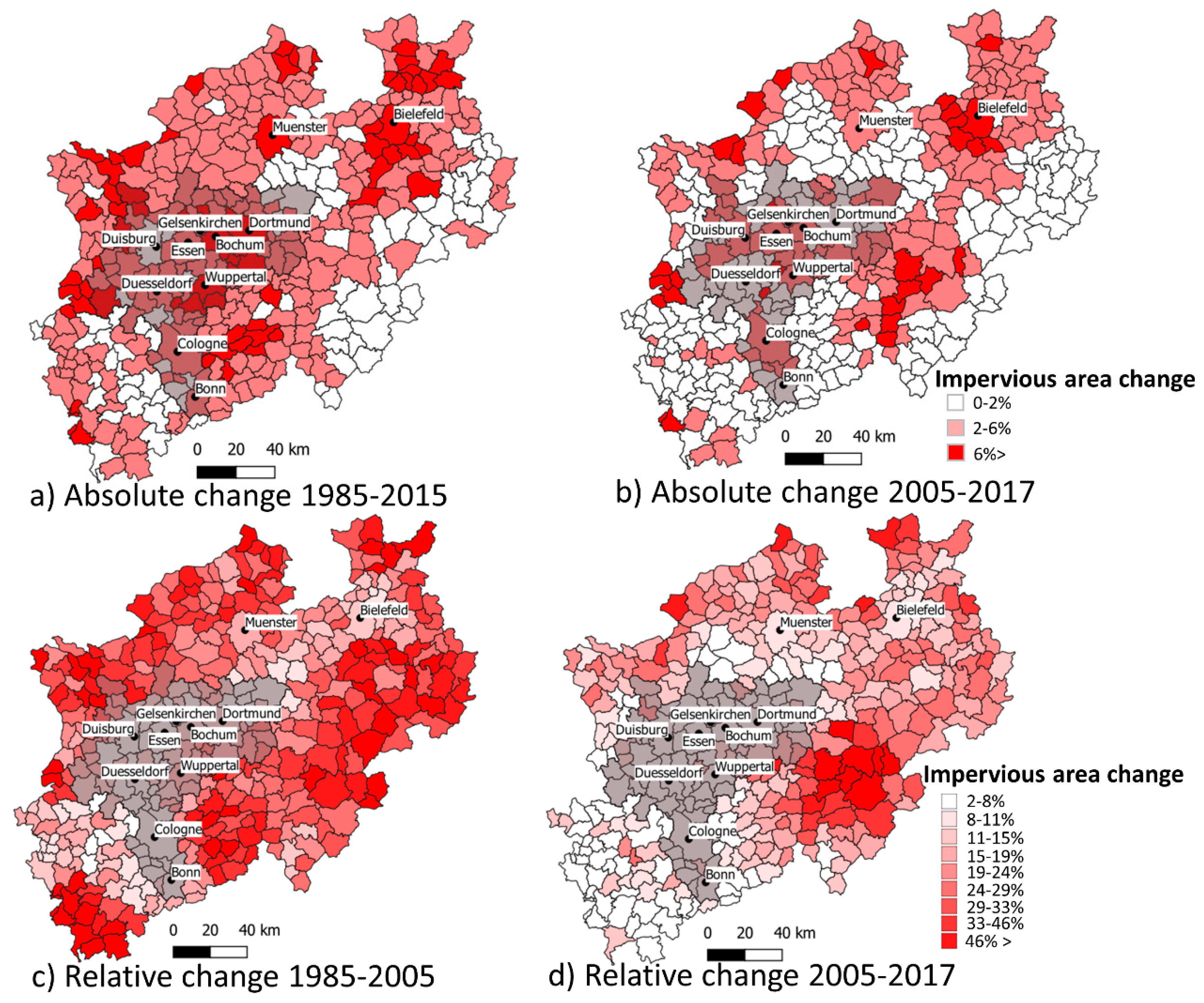
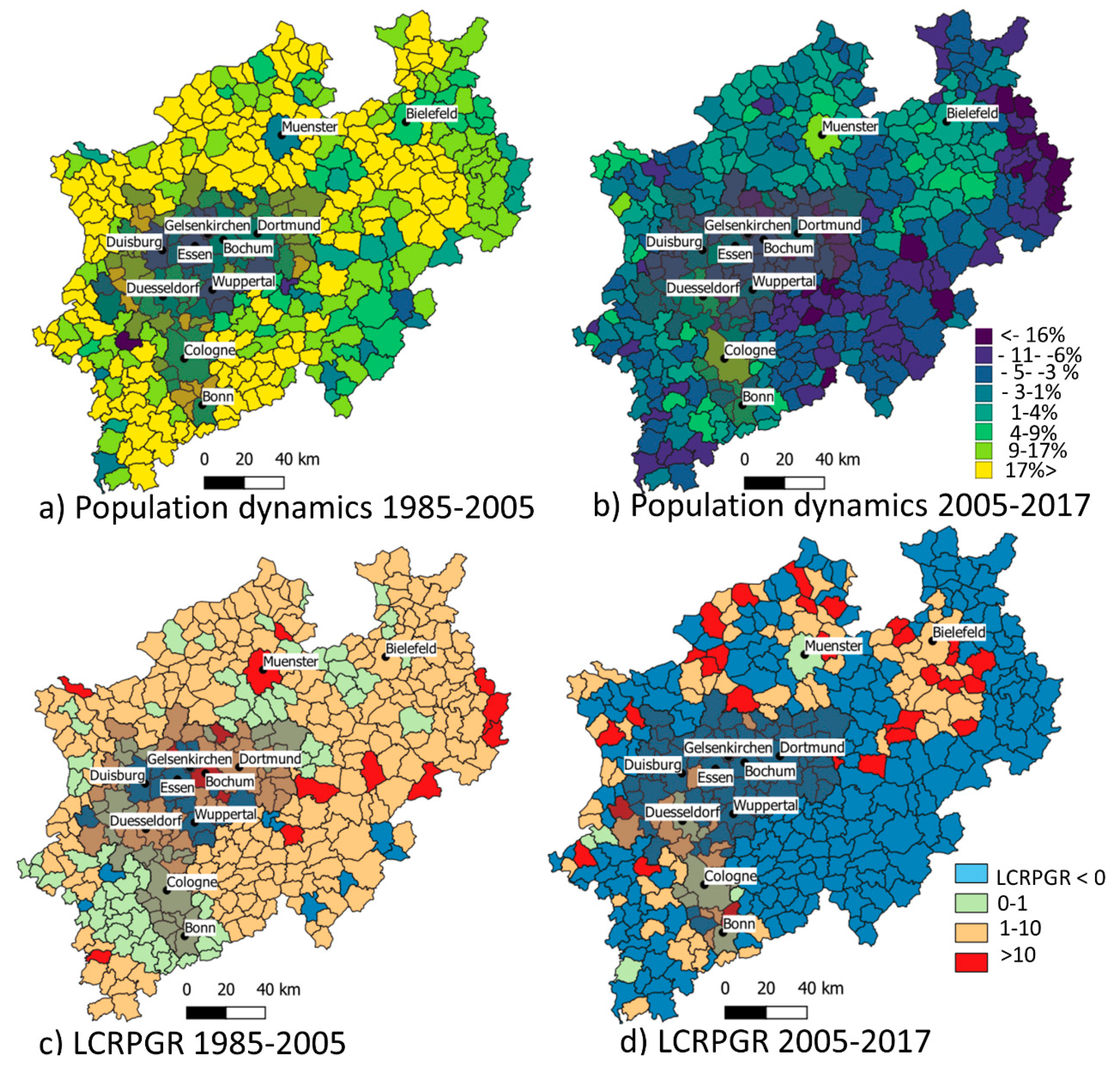
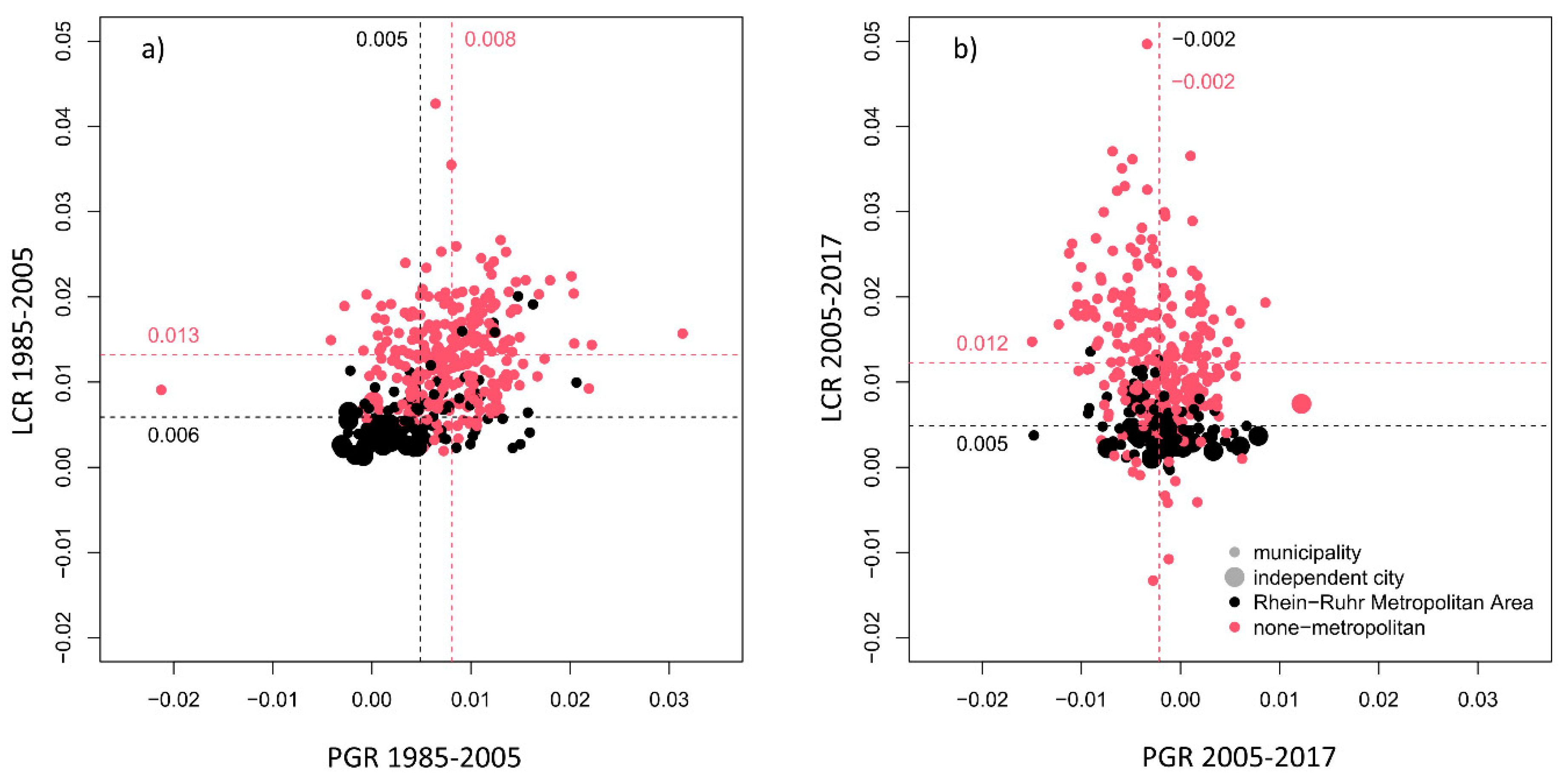
4.2. Land Consumption and Population Dynamics

Figure 7 shows the relationship between the LCR and PGR trends presented in the LCRPGR. LCRPGR estimates for the period 1985–2005 are positive in most municipalities. This shows parallel increase of both population growth and soil consumption rate. In various areas, the ratio varies between zero and one. In these municipalities, a simultaneous increase in the population growth rate can be observed. In the period 2005–2017, the proportion of municipalities that presented a negative estimate of LCRPGR was higher, showing the soil consumption increase combined with urban population reduction. This indicates that land use changes and population growth are not always in parallel, underlining the detachment of population growth as the main underlying cause of urban growth. Municipalities with high LCRPGR can be found in the peri-urban surroundings of the Rhine-Ruhr metropolitan region and in the rural areas in the Northern part. As a result, 1985–2005 was a period of rural growth (according to the population pattern in Figure 7a), while 2005–2017 was a period of urbanization (i.e., growth of urban population, rural exodus, Figure 7b).
Figure 8 shows LCR and PGR, extracted for municipalities, RRMA, independent cities and non-metropolitan regions. Land consumption mainly occurs in non-independent cities, i.e., rural areas, and has accelerated in some rural municipalities. Population growth was slower in RRMA than the rest in 1985–2005 but is equal in 2005–2019. However, PGR has generally decreased. The average land consumption has lowered slightly for both RRMA and other municipalities.
Using three imperviousness classes, distinct patterns have shown the densification processes and conversions from low and middle levels to high imperviousness from 1985 to 2017 (Figure 9). This is an advantage compared to one single urban class in the classification (Figure 6), which can omit patterns of the densification processes that can act as important indicators of sustainable growth. In general, densification is preferred over expansion and the development of new building areas since forests and agricultural areas can be preserved. Nevertheless, continuous increases in densification hold challenges, such as in logistics and urban climate [40]. This is the type of urban growth, which is the hardest to monitor with binary classification. The observation of the class low imperviousness and the transformation of that class to higher imperviousness levels provide the chance to observe densification of metropolitan regions, but also observe modification of land use for further ecosystem-oriented analyses. One of the main limitation of the study is the inaccuracies for the low imperviousness class, but they are still acceptable, considering the heterogeneity of the class and the spatial resolution of the dataset used. Nevertheless, our study allows land consumption information to be updated at a spatial scale adequate for land use planning at an administrative level. As opposed to existing datasets, our results reveal spatial patterns of densification and intensification within urban agglomerations. The approach considered the specific German situation, where the often conflicting interests in land use planning lead to small-scale changes and distinct patterns of densification in urban centers, and extensive land use conversion in the urban fringe. These processes are neither adequately addressed in existing global products nor in other approaches of urban change monitoring. As opposed to most published papers that often focus on urban areas with high growth rates, our study covers a heterogeneous region with predominantly small-scale urbanization, resulting in densification rather than more areal growth. We provide a methodology that allows us to detect and quantify these specific changes, which can have fundamental implications for socio-economic processes. As a result, the applied methodology contributes to urban mapping by offering a reliable way to account for changes with limited data and further extends the approach for SDG indicator estimation.
Although the applied approach showed potential for urban growth analyses, further investigations can be improved by integrating other datasets, such as night time lights. The addition of SAR data from TanDEM-X and Sentinel-1 can further delineate the urban structures and accurately reveal densification processes [73]. This study focused on the classification of imagery at a regional scale. In future studies, Landsat data can be complemented with Sentinel-2 and applied at a larger scale to derive LU/LC information at both high spatial and thematic resolution. Future research should focus on method transferability on multiple levels. The approach can be implemented and applied over the larger scale with the availability of the change detection algorithm on Google Earth Engine [74] and available Landsat time series.

5. Conclusions

This study presents an approach for automated retrospective LU/LC classification with the use of the spectral information of unchanged pixels. The method’s performance indicates that it is a promising approach for quantifying the changes in land use, including the derivation of several levels of impervious surfaces, with the use of reference data only for the baseline timestep. The analysis indicates a continuously growing imperviousness area during 1985–2017 in our study area. Further analysis of intensity showed the importance of identifying three imperviousness levels, which can better describe the densification processes of the urban areas in the study site. Using the approach, land consumption information was updated at a spatial scale, adequate for land use planning at an administrative level. By conducting an intensity analysis and the integration of population data, the spatial heterogeneity of urban expansion and population growth was assessed. We observed that the urban expansion rates considerably increased population growth rates in some of the regions in NRW, indicating more expansive urban growth patterns. Land consumption has accelerated in at least some of the rural municipalities. Furthermore, it is much lower in the RRMA as compared to the remaining municipalities. The analysis of LCRPGR showed that, especially for 2005–2017, land use change and population growth were not simultaneous. The former relationship of population growth and urban growth can be dismissed for the study area in Western Germany. This is an important finding as it proves that when it comes to SDG 11.3.1 urban, as well as rural areas are not maintaining an efficient land use policy, so that a sustainable settlement development until 2030 is hard to be seen in the Federal State of North Rhine-Westphalia. Especially the periurban regions are experiencing an inefficient settlement growth. The study highlights the applicability of earth observation data for accurately quantifying urban change for further sustainable targeted planning practices.

Author Contributions

Conceptualization, A.R., G.G. and F.T.; funding acquisition and supervision A.R. and C.J.; formal analysis, G.G., F.T., C.O. and A.R.; data curation, C.O., S.S. and B.T. All authors have read and agreed to the published version of the manuscript.

Funding

The project “Town and Country in the Flow—Network for the Creation of a sustainable Climate Landscape” (KlimNet) was funded with means of the Federal Ministry for the Environment, Nature Conservation and Nuclear Safety following a decision of the German Bundestag (funding code 67DAS098 ABC) within the German Strategy for Adaptation to Climate Change (Deutsche Anpassungsstrategie an den Klimawandel, DAS).

Data Availability Statement

The raw data used for this study (Landsat surface reflectance) can be acquired via USGS (https://earthexplorer.usgs.gov/ (accessed on 1 March 2021)). The reference data are subject to permission of third party (German Authoritative Topographic-Cartographic Information System). Additional demographic data were accessed from State Office Information and Technology North Rhine-Westphalia https://www.it.nrw/ (accessed on 1 March 2021).

Conflicts of Interest

The authors declare no conflict of interest.

References

  1. Song, X.-P.; Sexton, J.O.; Huang, C.; Channan, S.; Townshend, J.R. Characterizing the Magnitude, Timing and Duration of Urban Growth from Time Series of Landsat-Based Estimates of Impervious Cover. Remote Sens. Environ. 2016, 175, 1–13. [Google Scholar] [CrossRef]
  2. Liu, C.; Zhang, Q.; Luo, H.; Qi, S.; Tao, S.; Xu, H.; Yao, Y. An Efficient Approach to Capture Continuous Impervious Surface Dynamics Using Spatial-Temporal Rules and Dense Landsat Time Series Stacks. Remote Sens. Environ. 2019, 229, 114–132. [Google Scholar] [CrossRef]
  3. DESA UN World Urbanization Prospects: The 2018 Revision, Key Facts. New York, NY, USA. Available online: https://population.un.org/wup/Publications/ (accessed on 20 December 2018).
  4. El Mendili, L.; Puissant, A.; Chougrad, M.; Sebari, I. Towards a Multi-Temporal Deep Learning Approach for Mapping Urban Fabric Using Sentinel 2 Images. Remote Sens. 2020, 12, 423. [Google Scholar] [CrossRef] [Green Version]
  5. Li, W. Mapping Urban Impervious Surfaces by Using Spectral Mixture Analysis and Spectral Indices. Remote Sens. 2020, 12, 94. [Google Scholar] [CrossRef] [Green Version]
  6. Deng, C.; Zhu, Z. Continuous Subpixel Monitoring of Urban Impervious Surface Using Landsat Time Series. Remote Sens. Environ. 2020, 238, 110929. [Google Scholar] [CrossRef]
  7. Weng, Q. Remote Sensing of Impervious Surfaces in the Urban Areas: Requirements, Methods, and Trends. Remote Sens. Environ. 2012, 117, 34–49. [Google Scholar] [CrossRef]
  8. Li, W.; El-Askary, H.; Lakshmi, V.; Piechota, T.; Struppa, D. Earth Observation and Cloud Computing in Support of Two Sustainable Development Goals for the River Nile Watershed Countries. Remote Sens. 2020, 12, 1391. [Google Scholar] [CrossRef]
  9. Schiavina, M.; Melchiorri, M.; Corbane, C.; Florczyk, A.J.; Freire, S.; Pesaresi, M.; Kemper, T. Multi-Scale Estimation of Land Use Efficiency (SDG 11.3.1) across 25 Years Using Global Open and Free Data. Sustainability 2019, 11, 5674. [Google Scholar] [CrossRef] [Green Version]
  10. Wang, Y.; Huang, C.; Feng, Y.; Zhao, M.; Gu, J. Using Earth Observation for Monitoring SDG 11.3.1-Ratio of Land Consumption Rate to Population Growth Rate in Mainland China. Remote Sens. 2020, 12, 357. [Google Scholar] [CrossRef] [Green Version]
  11. Angel, S.; Parent, J.; Civco, D.L.; Blei, A.M. Making Room for a Planet of Cities; Lincoln Institute of Land Policy: Cambridge, MA, USA, 2011; Available online: http://www.lincolninst.edu/pubs/1880_Making-Room-for-a-Planet-of-Cities-urban-expansion (accessed on 24 April 2021).
  12. UNSTATS. Indicator 11.3.1. Available online: Https://Unstats.Un.Org/Sdgs/Metadata/Files/Metadata-08-05-01.Pdf (accessed on 10 April 2021).
  13. Mudau, N.; Mwaniki, D.; Tsoeleng, L.; Mashalane, M.; Beguy, D.; Ndugwa, R. Assessment of SDG Indicator 11.3.1 and Urban Growth Trends of Major and Small Cities in South Africa. Sustainability 2020, 12, 7063. [Google Scholar] [CrossRef]
  14. Ravanelli, R.; Nascetti, A.; Cirigliano, R.V.; Di Rico, C.; Leuzzi, G.; Monti, P.; Crespi, M. Monitoring the Impact of Land Cover Change on Surface Urban Heat Island through Google Earth Engine: Proposal of a Global Methodology, First Applications and Problems. Remote Sens. 2018, 10, 1488. [Google Scholar] [CrossRef] [Green Version]
  15. van der Linden, S.; Okujeni, A.; Canters, F.; Degerickx, J.; Heiden, U.; Hostert, P.; Priem, F.; Somers, B.; Thiel, F. Imaging Spectroscopy of Urban Environments. Surv. Geophys. 2019, 40, 471–488. [Google Scholar] [CrossRef] [Green Version]
  16. Henits, L.; Jürgens, C.; Mucsi, L. Seasonal Multitemporal Land-Cover Classification and Change Detection Analysis of Bochum, Germany, Using Multitemporal Landsat TM Data. Int. J. Remote Sens. 2016, 37, 3439–3454. [Google Scholar] [CrossRef]
  17. Liu, X.; Huang, Y.; Xu, X.; Li, X.; Li, X.; Ciais, P.; Lin, P.; Gong, K.; Ziegler, A.D.; Chen, A. High-Spatiotemporal-Resolution Mapping of Global Urban Change from 1985 to 2015. Nat. Sustain. 2020, 3, 564–570. [Google Scholar] [CrossRef]
  18. Weigand, M.; Staab, J.; Wurm, M.; Taubenböck, H. Spatial and Semantic Effects of LUCAS Samples on Fully Automated Land Use/Land Cover Classification in High-Resolution Sentinel-2 Data. Int. J. Appl. Earth Obs. Geoinf. 2020, 88, 102065. [Google Scholar] [CrossRef]
  19. Fan, W.; Wu, C.; Wang, J. Improving Impervious Surface Estimation by Using Remote Sensed Imagery Combined With Open Street Map Points-of-Interest (POI) Data. IEEE J. Sel. Top. Appl. Earth Obs. Remote Sens. 2019, 12, 4265–4274. [Google Scholar] [CrossRef]
  20. Kaspersen, P.S.; Fensholt, R.; Drews, M. Using Landsat Vegetation Indices to Estimate Impervious Surface Fractions for European Cities. Remote Sens. 2015, 7, 8224–8249. [Google Scholar] [CrossRef] [Green Version]
  21. O’Connor, B.; Moul, K.; Pollini, B.; de Lamo, X.; Simonson, W. Compendium of Earth Observation Contributions to the SDG Targets and Indicators 2020. 2020. Available online: https://eo4society.esa.int/wp-content/uploads/2021/01/EO_Compendium-for-SDGs.pdf (accessed on 20 April 2021).
  22. Deng, Y.; Fan, F.; Chen, R. Extraction and Analysis of Impervious Surfaces Based on a Spectral Un-Mixing Method Using Pearl River Delta of China Landsat TM/ETM+ Imagery from 1998 to 2008. Sensors 2012, 12, 1846–1862. [Google Scholar] [CrossRef] [Green Version]
  23. Deliry, S.I.; Avdan, Z.Y.; Avdan, U. Extracting Urban Impervious Surfaces from Sentinel-2 and Landsat-8 Satellite Data for Urban Planning and Environmental Management. Environ. Sci. Pollut. Res. 2021, 28, 6572–6586. [Google Scholar] [CrossRef]
  24. Esch, T.; Himmler, V.; Schorcht, G.; Thiel, M.; Wehrmann, T.; Bachofer, F.; Conrad, C.; Schmidt, M.; Dech, S. Large-Area Assessment of Impervious Surface Based on Integrated Analysis of Single-Date Landsat-7 Images and Geospatial Vector Data. Remote Sens. Environ. 2009, 113, 1678–1690. [Google Scholar] [CrossRef]
  25. Wu, C.; Du, B.; Cui, X.; Zhang, L. A Post-Classification Change Detection Method Based on Iterative Slow Feature Analysis and Bayesian Soft Fusion. Remote Sens. Environ. 2017, 199, 241–255. [Google Scholar] [CrossRef]
  26. Hecheltjen, A.; Thonfeld, F.; Menz, G. Recent Advances in Remote Sensing Change Detection—A Review. Land Use Land Cover Mapp. Eur. 2014, 145–178. [Google Scholar] [CrossRef]
  27. Hassan, M.M. Monitoring Land Use/Land Cover Change, Urban Growth Dynamics and Landscape Pattern Analysis in Five Fastest Urbanized Cities in Bangladesh. Remote Sens. Appl. Soc. Environ. 2017, 7, 69–83. [Google Scholar] [CrossRef]
  28. Yang, A.; Sun, G. Landsat-Based Land Cover Change in the Beijing-Tianjin-Tangshan Urban Agglomeration in 1990, 2000 and 2010. Isprs Int. J. Geo-Inf. 2017, 6, 59. [Google Scholar] [CrossRef] [Green Version]
  29. Schug, F.; Okujeni, A.; Hauer, J.; Hostert, P.; Nielsen, J.Ø.; van der Linden, S. Mapping Patterns of Urban Development in Ouagadougou, Burkina Faso, Using Machine Learning Regression Modeling with Bi-Seasonal Landsat Time Series. Remote Sens. Environ. 2018, 210, 217–228. [Google Scholar] [CrossRef]
  30. Pesaresi, M.; Huadong, G.; Blaes, X.; Ehrlich, D.; Ferri, S.; Gueguen, L.; Halkia, M.; Kauffmann, M.; Kemper, T.; Lu, L.; et al. A Global Human Settlement Layer From Optical HR/VHR RS Data: Concept and First Results. IEEE J. Sel. Top. Appl. Earth Obs. Remote Sens. 2013, 6, 2102–2131. [Google Scholar] [CrossRef]
  31. Esch, T.; Heldens, W.; Hirner, A.; Keil, M.; Marconcini, M.; Roth, A.; Zeidler, J.; Dech, S.; Strano, E. Breaking New Ground in Mapping Human Settlements from Space—The Global Urban Footprint. ISPRS J. Photogramm. Remote Sens. 2017, 134, 30–42. [Google Scholar] [CrossRef] [Green Version]
  32. Marconcini, M.; Metz-Marconcini, A.; Üreyen, S.; Palacios-Lopez, D.; Hanke, W.; Bachofer, F.; Zeidler, J.; Esch, T.; Gorelick, N.; Kakarla, A.; et al. Outlining Where Humans Live, the World Settlement Footprint 2015. Sci. Data 2020, 7, 242. [Google Scholar] [CrossRef] [PubMed]
  33. Lefebvre, A.; Sannier, C.; Corpetti, T. Monitoring Urban Areas with Sentinel-2A Data: Application to the Update of the Copernicus High Resolution Layer Imperviousness Degree. Remote Sens. 2016, 8, 606. [Google Scholar] [CrossRef] [Green Version]
  34. Melchiorri, M.; Florczyk, A.J.; Freire, S.; Schiavina, M.; Pesaresi, M.; Kemper, T. Unveiling 25 Years of Planetary Urbanization with Remote Sensing: Perspectives from the Global Human Settlement Layer. Remote Sens. 2018, 10, 768. [Google Scholar] [CrossRef] [Green Version]
  35. Siedentop, S.; Fina, S. Monitoring Urban Sprawl in Germany: Towards a GIS-Based Measurement and Assessment Approach. J. Land Use Sci. 2010, 5, 73–104. [Google Scholar] [CrossRef]
  36. European Environmental Agency (EEA) Urban Sprawl in Europe Joint EEA-FOEN Repor 2016; European Environmental Agency—Swiss Federal office for the Environment: Luxembourg, 2016; ISBN 978-92-9213-738-0.
  37. Hoymann, J.; Goetzke, R. Simulation and Evaluation of Urban Growth for Germany Including Climate Change Mitigation and Adaptation Measures. ISPRS Int. J. Geo-Inf. 2016, 5, 101. [Google Scholar] [CrossRef] [Green Version]
  38. Arsanjani, J.J.; See, L.; Tayyebi, A. Assessing the Suitability of GlobeLand30 for Mapping Land Cover in Germany. Int. J. Digit. Earth 2016, 9, 873–891. [Google Scholar] [CrossRef] [Green Version]
  39. European Environmental Agency (EEA) Country Fact Sheet: Land Cover 2012. 2012. Available online: https://www.eea.europa.eu/themes/landuse/land-cover-country-fact-sheets/land-cover-country-fact-sheets-2012/de-germany-landcover-2012.pdf/view (accessed on 20 April 2021).
  40. Rienow, A.; Schneevoigt, N.J.; Thonfeld, F. Quantification and Prediction of Land Consumption and Its Climate Effects in the Rhineland Metropolitan Area Based on Multispectral Satellite Data and Land-Use Modelling 1975–2030. Spat. Anal. Model. Plan. 2018. [Google Scholar] [CrossRef] [Green Version]
  41. Bezirksregierung Köln Erläuterung Zu Abweichungen in Der Flächenerhebung Nach Art Der Tatsächlichen Nutzung Nach Dem Umstieg von ALK/ALB Nach ALKIS in NRW; Bezirksregierung Köln: Cologne, Germany, 2020.
  42. IT. NRW Data Licence Germany—Attribution—Version 2.0. 2020. Available online: https://www.it.nrw/ (accessed on 1 March 2021).
  43. Zhu, Z.; Wang, S.; Woodcock, C.E. Improvement and Expansion of the Fmask Algorithm: Cloud, Cloud Shadow, and Snow Detection for Landsats 4–7, 8, and Sentinel 2 Images. Remote Sens. Environ. 2015, 159, 269–277. [Google Scholar] [CrossRef]
  44. Tucker, C.J. Red and Photographic Infrared Linear Combinations for Monitoring Vegetation. Remote Sens. Environ. 1979, 8, 127–150. [Google Scholar] [CrossRef] [Green Version]
  45. Juergens, C.; Meyer-Heß, M.F. Application of NDVI in Environmental Justice, Health and Inequality Studies—Potential and Limitations in Urban Environments. Preprints 2020, 2020080499. [Google Scholar] [CrossRef]
  46. Mcfeeters, S.K. The Use of the Normalized Difference Water Index (NDWI) in the Delineation of Open Water Features. Int. J. Remote Sens. 1996, 17, 1425–1432. [Google Scholar] [CrossRef]
  47. Crist, E.P.; Cicone, R.C. A Physically-Based Transformation of Thematic Mapper Data—The TM Tasseled Cap. IEEE Trans. Geosci. Remote Sens. 1984, GE-22, 256–263. [Google Scholar] [CrossRef]
  48. Azzari, G.; Lobell, D.B. Landsat-Based Classification in the Cloud: An Opportunity for a Paradigm Shift in Land Cover Monitoring. Remote Sens. Environ. 2017, 202, 64–74. [Google Scholar] [CrossRef]
  49. Esch, T.; Metz, A.; Marconcini, M.; Keil, M. Combined Use of Multi-Seasonal High and Medium Resolution Satellite Imagery for Parcel-Related Mapping of Cropland and Grassland. Int. J. Appl. Earth Obs. Geoinf. 2014, 28, 230–237. [Google Scholar] [CrossRef]
  50. Hansen, M.C.; Egorov, A.; Potapov, P.V.; Stehman, S.V.; Tyukavina, A.; Turubanova, S.A.; Roy, D.P.; Goetz, S.J.; Loveland, T.R.; Ju, J. Monitoring Conterminous United States (CONUS) Land Cover Change with Web-Enabled Landsat Data (WELD). Remote Sens. Environ. 2014, 140, 466–484. [Google Scholar] [CrossRef] [Green Version]
  51. Thonfeld, F.; Steinbach, S.; Muro, J.; Kirimi, F. Long-Term Land Use/Land Cover Change Assessment of the Kilombero Catchment in Tanzania Using Random Forest Classification and Robust Change Vector Analysis. Remote Sens. 2020, 12, 1057. [Google Scholar] [CrossRef] [Green Version]
  52. Breiman, L. Random Forests. Mach. Learn. 2001, 45, 5–32. [Google Scholar] [CrossRef] [Green Version]
  53. Huang, H.; Chen, Y.; Clinton, N.; Wang, J.; Wang, X.; Liu, C.; Gong, P.; Yang, J.; Bai, Y.; Zheng, Y.; et al. Mapping Major Land Cover Dynamics in Beijing Using All Landsat Images in Google Earth Engine. Remote Sens. Environ. 2017, 202, 166–176. [Google Scholar] [CrossRef]
  54. Li, M.; Zang, S.; Zhang, B.; Li, S.; Wu, C. A Review of Remote Sensing Image Classification Techniques: The Role of Spatio-Contextual Information. Eur. J. Remote Sens. 2014, 47, 389–411. [Google Scholar] [CrossRef]
  55. Pal, M. Random Forest Classifier for Remote Sensing Classification. Int. J. Remote Sens. 2005, 26, 217–222. [Google Scholar] [CrossRef]
  56. Liaw, A.; Wiener, M. Classification and Regression by RandomForest. R. News 2002, 2, 18–22. [Google Scholar]
  57. R Core Team. R: A Language and Environment for Statistical Computing; R Foundation for Statistical Computing; R Core Team: Vienna, Austria, 2020. [Google Scholar]
  58. Goetzke, R.; Judex, M.; Braun, M.; Menz, G. Evaluation of Driving Forces of Land-Use Change and Urban Growth in North Rhine-Westphalia (Germany). In Proceedings of the 2007 IEEE International Geoscience and Remote Sensing Symposium, Barcelona, Spain, 23–28 July 2007; pp. 3425–3428. [Google Scholar]
  59. Qin, Y.; Xiao, X.; Dong, J.; Chen, B.; Liu, F.; Zhang, G.; Zhang, Y.; Wang, J.; Wu, X. Quantifying Annual Changes in Built-up Area in Complex Urban-Rural Landscapes from Analyses of PALSAR and Landsat Images. ISPRS J. Photogramm. Remote Sens. 2017, 124, 89–105. [Google Scholar] [CrossRef] [Green Version]
  60. Büttner, G. CORINE Land Cover and Land Cover Change Products. In Land Use and Land Cover Mapping in Europe: Practices & Trends; Manakos, I., Braun, M., Eds.; Remote Sensing and Digital Image Processing; Springer: Dordrecht, The Netherlands, 2014; pp. 55–74. ISBN 978-94-007-7969-3. [Google Scholar]
  61. Nielsen, A.A. The Regularized Iteratively Reweighted MAD Method for Change Detection in Multi-and Hyperspectral Data. IEEE Trans. Image Process. 2007, 16, 463–478. [Google Scholar] [CrossRef] [Green Version]
  62. Canty, M.J.; Nielsen, A.A. Automatic Radiometric Normalization of Multitemporal Satellite Imagery with the Iteratively Re-Weighted MAD Transformation. Remote Sens. Environ. 2008, 112, 1025–1036. [Google Scholar] [CrossRef] [Green Version]
  63. Marpu, P.R.; Gamba, P.; Canty, M.J. Improving Change Detection Results of IR-MAD by Eliminating Strong Changes. IEEE Geosci. Remote Sens. Lett. 2011, 8, 799–803. [Google Scholar] [CrossRef]
  64. Canty, M.J.; Nielsen, A.A. Linear and Kernel Methods for Multivariate Change Detection. Comput. Geosci. 2012, 38, 107–114. [Google Scholar] [CrossRef]
  65. Congalton, R.G. A Review of Assessing the Accuracy of Classifications of Remotely Sensed Data. Remote Sens. Environ. 1991, 37, 35–46. [Google Scholar] [CrossRef]
  66. Incora (Inwertsetzung von Copernicus-Daten für die Raumbeobachtung Germany 2019—Land Cover Based on Sentinel-2 Data—Mundialis. 2020. Available online: https://www.mundialis.de/de/deutschland-2019-landbedeckung-auf-basis-von-sentinel-2-daten (accessed on 1 March 2021).
  67. Weigand, M.; Wurm, M. Land Cover DE—Sentinel-2—Germany, 2015. 2020. Available online: https://geoservice.dlr.de/data-assets/1ccmlap3mn39.htm (accessed on 10 April 2021).
  68. Badmos, O.S.; Rienow, A.; Callo-Concha, D.; Greve, K.; Jürgens, C. Urban Development in West Africa—Monitoring and Intensity Analysis of Slum Growth in Lagos: Linking Pattern and Process. Remote Sens. 2018, 10, 1044. [Google Scholar] [CrossRef] [Green Version]
  69. Aldwaik, S.Z.; Pontius, R.G. Intensity Analysis to Unify Measurements of Size and Stationarity of Land Changes by Interval, Category, and Transition. Landsc. Urban Plan. 2012, 106, 103–114. [Google Scholar] [CrossRef]
  70. Sang, X.; Guo, Q.; Wu, X.; Fu, Y.; Xie, T.; He, C.; Zang, J. Intensity and Stationarity Analysis of Land Use Change Based on CART Algorithm. Sci. Rep. 2019, 9, 12279. [Google Scholar] [CrossRef] [PubMed] [Green Version]
  71. Nicolau, R.; David, J.; Caetano, M.; Pereira, J.M.C. Ratio of Land Consumption Rate to Population Growth Rate—Analysis of Different Formulations Applied to Mainland Portugal. ISPRS Int. J. Geo-Inf. 2019, 8, 10. [Google Scholar] [CrossRef] [Green Version]
  72. BBSR (Bundesinstitut für Bau-, Stadt- und Raumforschung) Studie Zum Monitoring Der Flächeninanspruchnahme—Evaluation Der Einschlägigen Datenbasis. 2020. Available online: https://www.bbsr.bund.de/BBSR/DE/forschung/programme/refo/raumordnung/2013/MonitoringFlaecheninanspruchnahme_Evaluation/01_Start.html (accessed on 20 April 2021).
  73. Zhou, T.; Li, Z.; Pan, J. Multi-Feature Classification of Multi-Sensor Satellite Imagery Based on Dual-Polarimetric Sentinel-1A, Landsat-8 OLI, and Hyperion Images for Urban Land-Cover Classification. Sensors 2018, 18, 373. [Google Scholar] [CrossRef] [PubMed] [Green Version]
  74. Canty, D.M. Mortcanty/Earthengine. 2021. Available online: https://github.com/mortcanty/earthengine (accessed on 20 April 2021).
Figure 1. North Rhine-Westphalia (NRW), western Germany with the highlighted Rhine-Ruhr Metropolitan Area (RRMA) and cities with big population.
Remotesensing 13 01694 g001
Figure 2. Workflow for land use classification presented for baseline year and 2015. For the preceding timesteps, the changes are calculated with the last image as the reference, and the ATKIS data are limited to the unchanged areas between two consecutive time steps.
Remotesensing 13 01694 g002
Figure 3. (a) The level of imperviousness for 2017 based on ATKIS data and RF regression, and (b) resulted land use map for 2017 baseline time step.
Remotesensing 13 01694 g003
Figure 4. Sankey plot for land-use changes observed in NRW from 1985 to 2017.
Remotesensing 13 01694 g004
Figure 5. Category level gains and losses for three imperviousness classes (dashed lines represent the threshold of uniform intensity across the spatial extent for each time interval).
Remotesensing 13 01694 g005
Figure 6. Changes in urbanization in NRW: Absolute change in between 1985–2005 (a) and 2005–2017 (b) and relative change between 1985–2005 (c) and 2005–2017 (d).
Remotesensing 13 01694 g006
Figure 7. Changes in population in NRW between 1985–2005 (a) and between 2005–2017 (b) and LCRPGR for the period 1985–2005 (c) and 2005–2017 (d).
Remotesensing 13 01694 g007
Figure 8. The scatter plots of LCR and PGR in (a) 1985–2005 and (b) 2005–2017.
Remotesensing 13 01694 g008
Figure 9. Changes in imperviousness level during the 32 years in NRW and for three selected cities, namely Dortmund, Cologne, and Duisburg.
Remotesensing 13 01694 g009
Table 1. Input variables used in LU/LC classification.
InputDescriptionCompositing
NDVINormalized difference vegetation index
NDWINormalized difference water index
TCCTasseled Cap Components (greenness, wetness, and brightness)Minimum, maximum, 10th, 25th, 50th, 75th, 80th and 90th percentile, mean over growing season (April-September) and year
Landsat TM, ETM+ and OLI bands Green, Blue, Red, NIR, SWIR1, SWIR2
Table 2. Accuracies of obtained maps.
YearOAPA for Low, Middle, and High Imperviousness ClassUA for Low, Middle, and High Imperviousness ClassAccuracies for Aggregated Urban AreaAccuracies for Aggregated Non-Urban Areas
PAUAPAUA
201789.0%89.3 90.5 94.489.4 90.5 94.496.393.0492.796.2
201587.0%77.9 93.9 90.181.5 90.7 90.194.691.390.994.7
201080.0%62.9 77.9 90.569.3 83.2 87.593.190.791.292.3
200579.1%82.9 76.2 89.978.2 92.4 82.694.892.194.696.7
200080.2%63.1 78.1 90.269.1 83.5 87.893.19696.293.3
199075.3%54.9 67.6 90.165.1 79.7 80.891.395.895.891.4
198577.3%61.1 69.8 87.474.5 75.7 82.987.795.996.188.3
Table 3. Intensity of change.
Intensity Change Category Time IntervalAnnual Intensity of Change (%)
Interval level1985–20051.71
2005–20172.72
Transition level1985–2005From Low to middle 0.49
From low to high 0.32
From middle to high 1.16
2005–2017From low to middle 1.38
From low to high 0.24
From middle high 0.62
Publisher’s Note: MDPI stays neutral with regard to jurisdictional claims in published maps and institutional affiliations.

