A Scalable Machine Learning Pipeline for Paddy Rice Classification Using Multi-Temporal Sentinel Data

 , , ,
, , ,  and
and
Abstract
:
1. Introduction
2. Materials
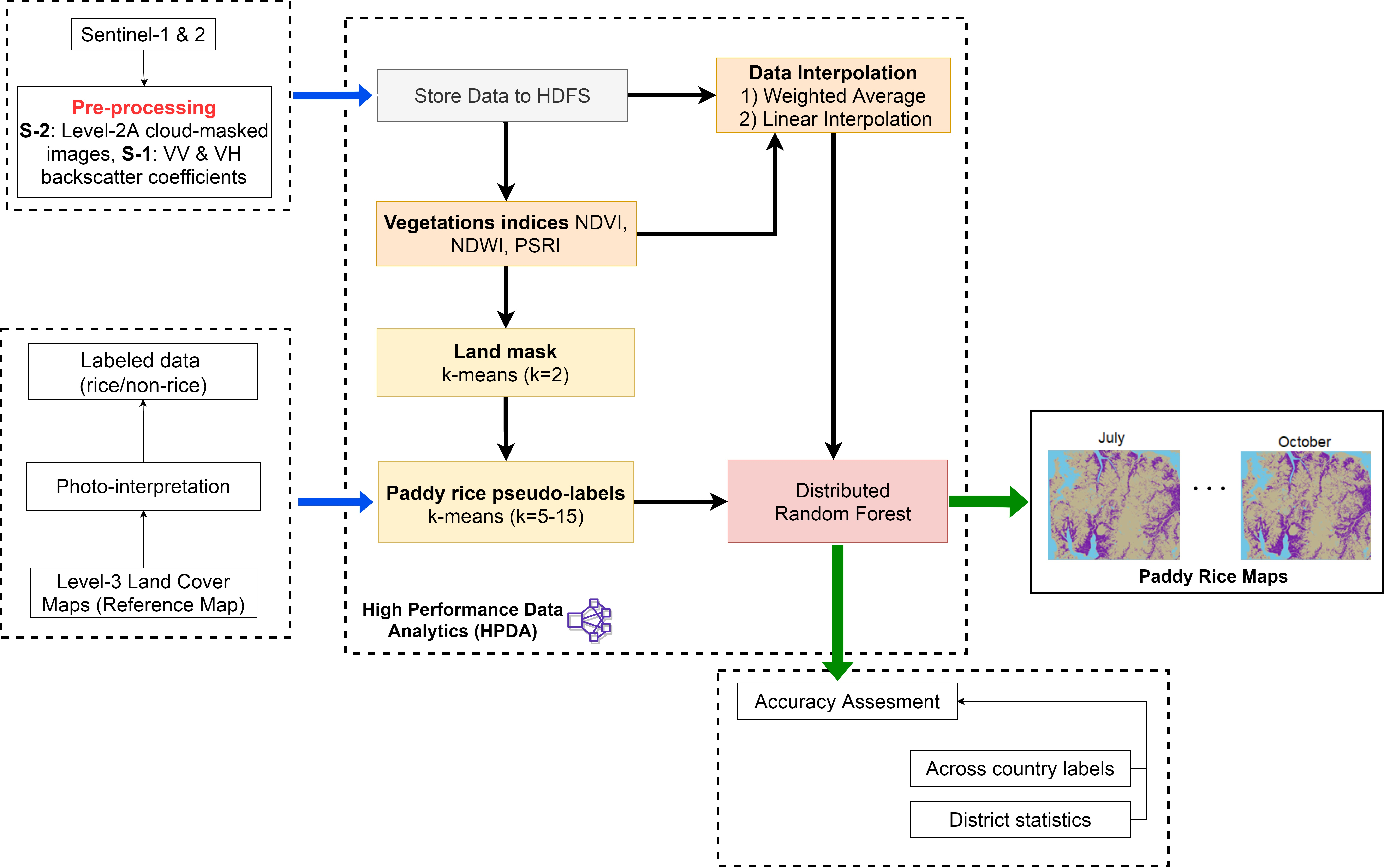
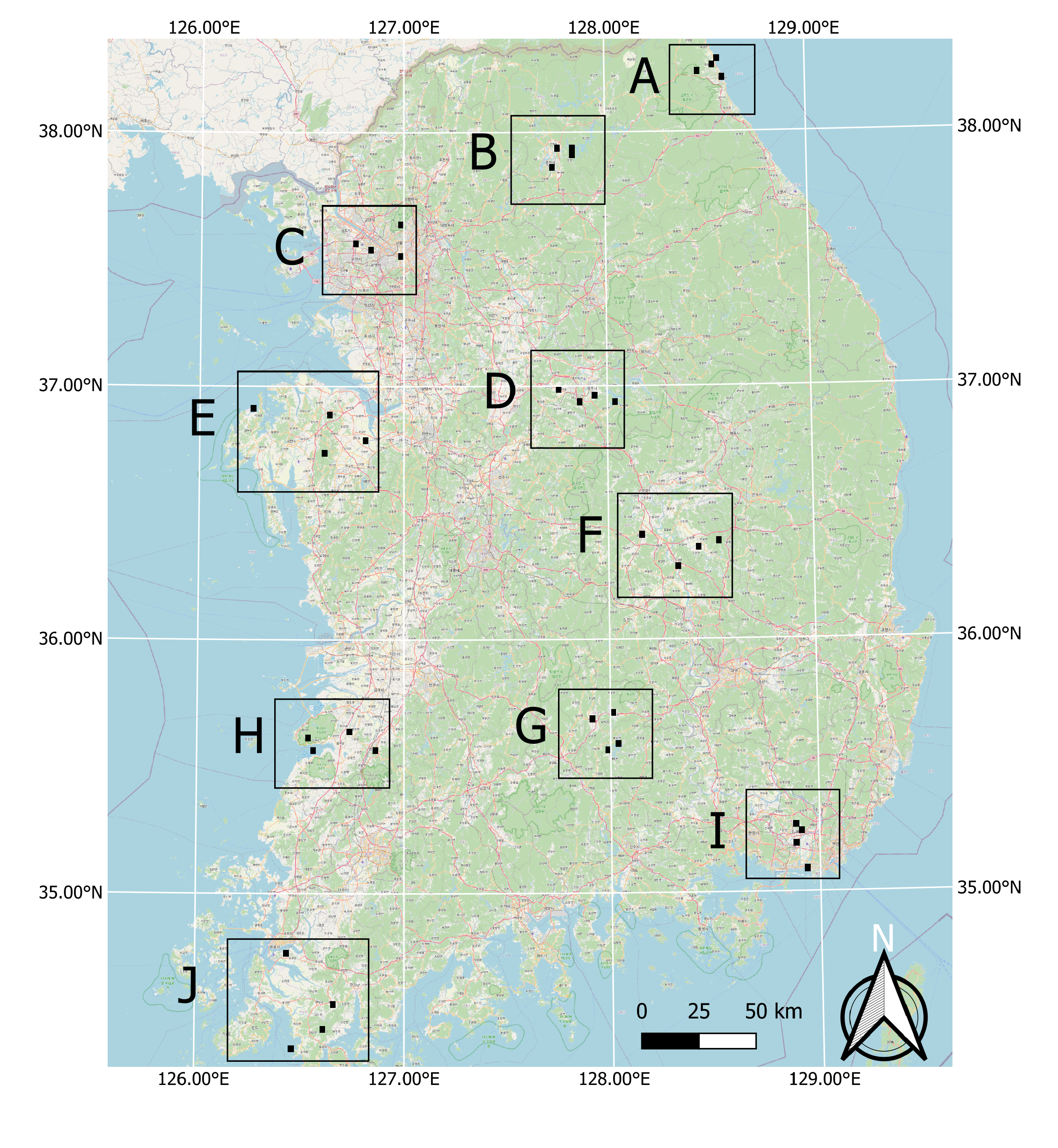
2.1. Study Area
2.2. Satellite Data
2.2.1. Sentinel-1 Data
2.2.2. Sentinel-2 Data
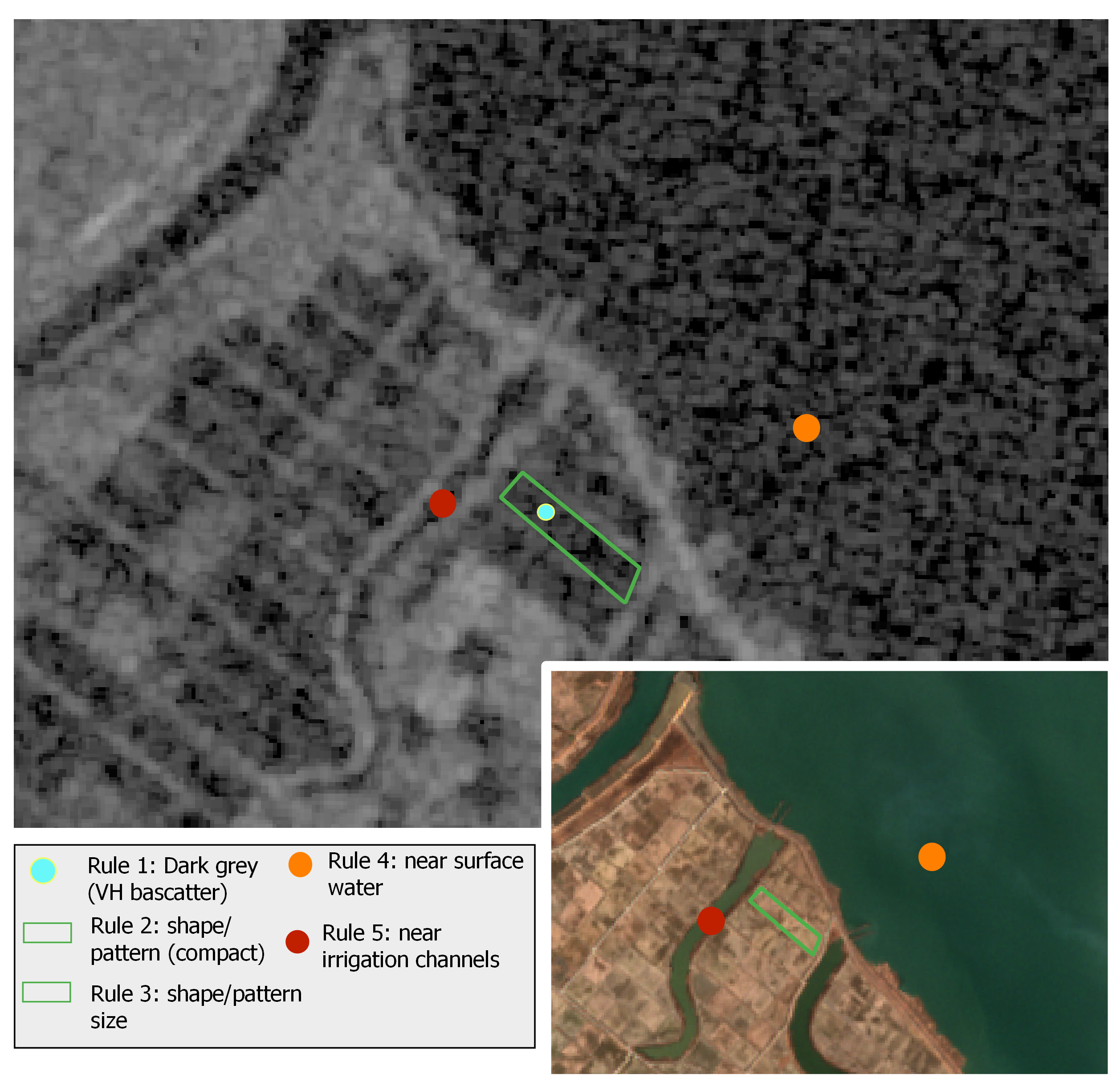
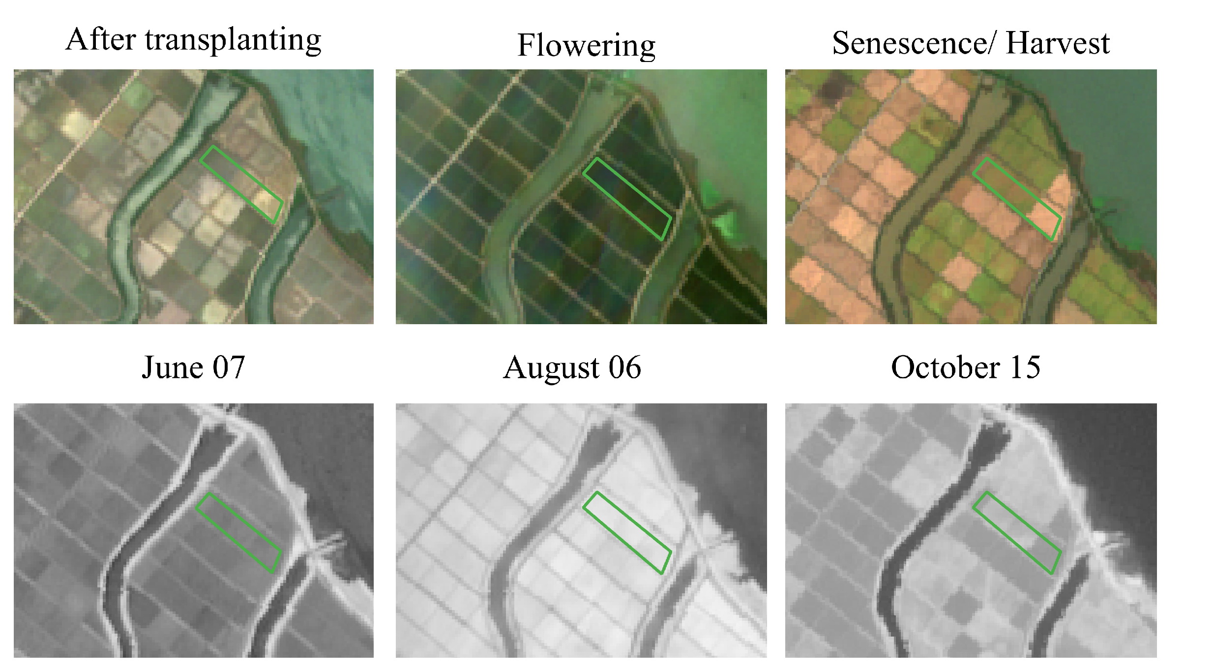
2.3. Labeled Data
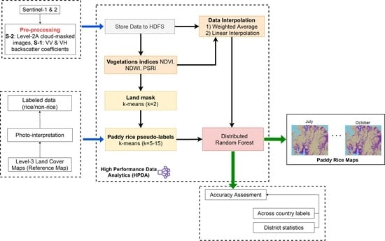
3. Methods
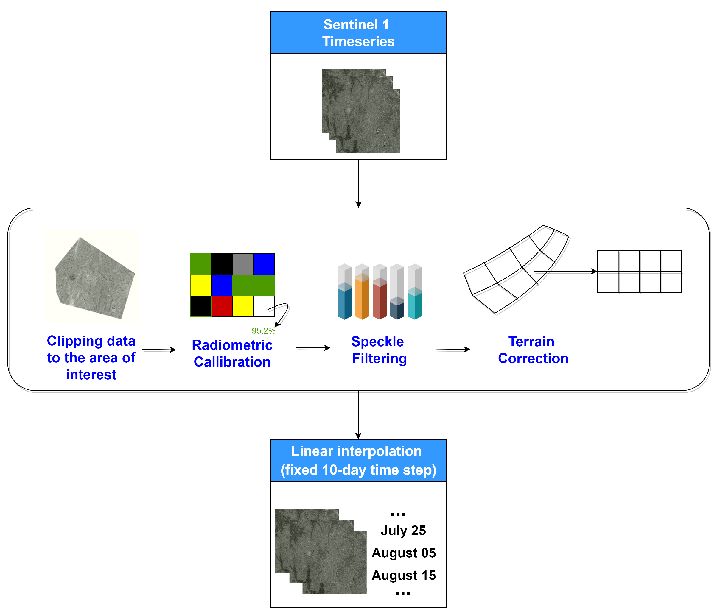
3.1. Sentinel-2 Time-Series Interpolation
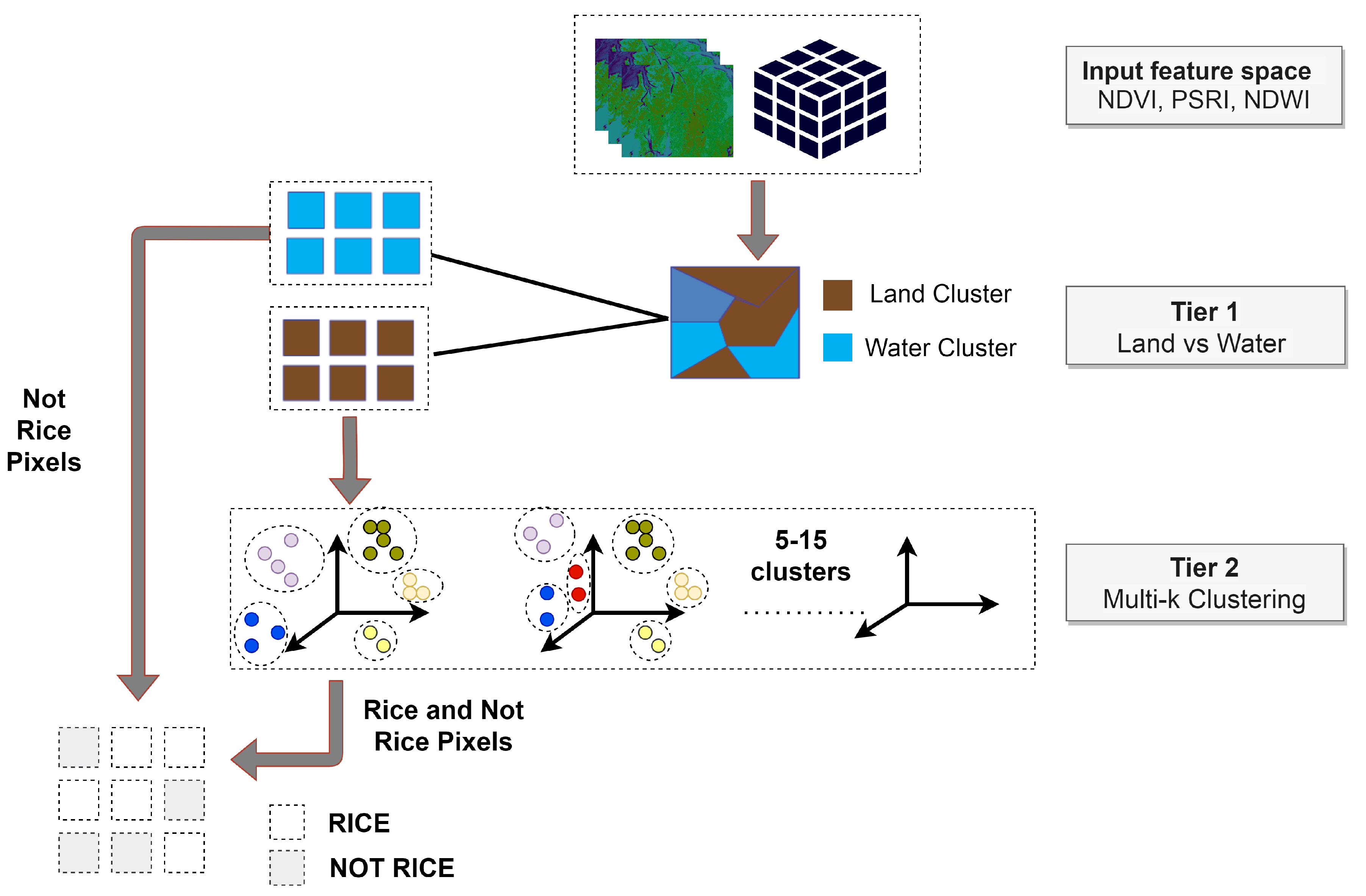
3.2. Pseudo-Labeling
3.3. Model Performance Evaluation
3.4. Supervised Classification Using Pseudo-Labels
4. Results
4.1. K-Means Clustering
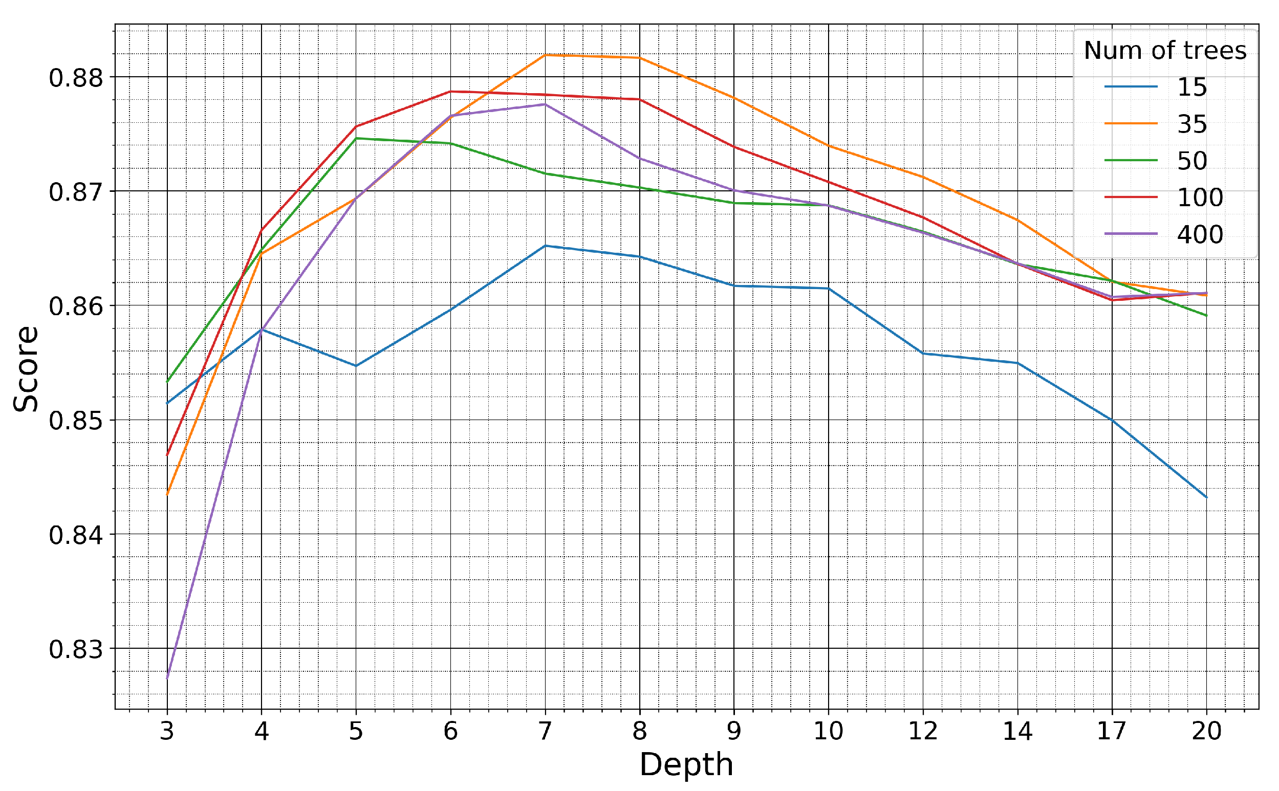
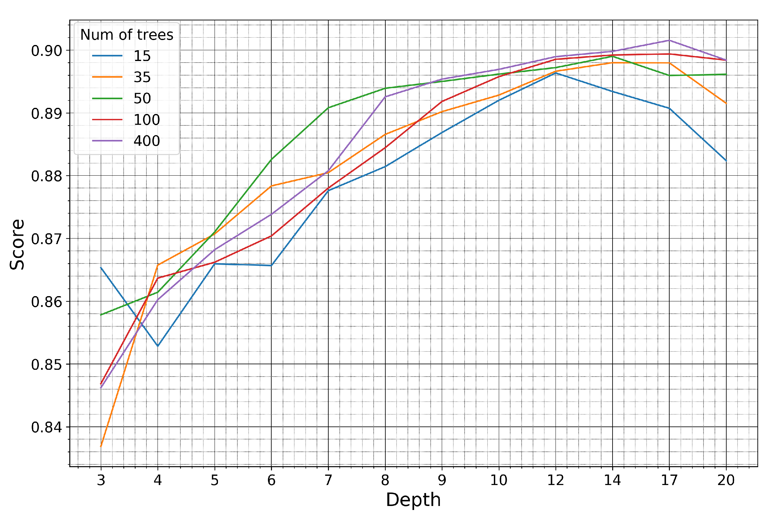
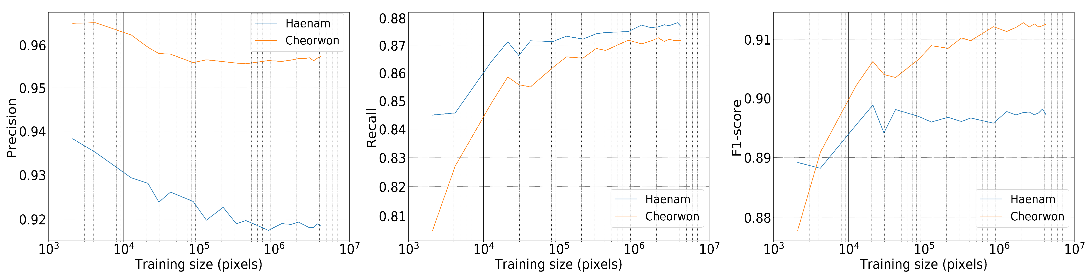
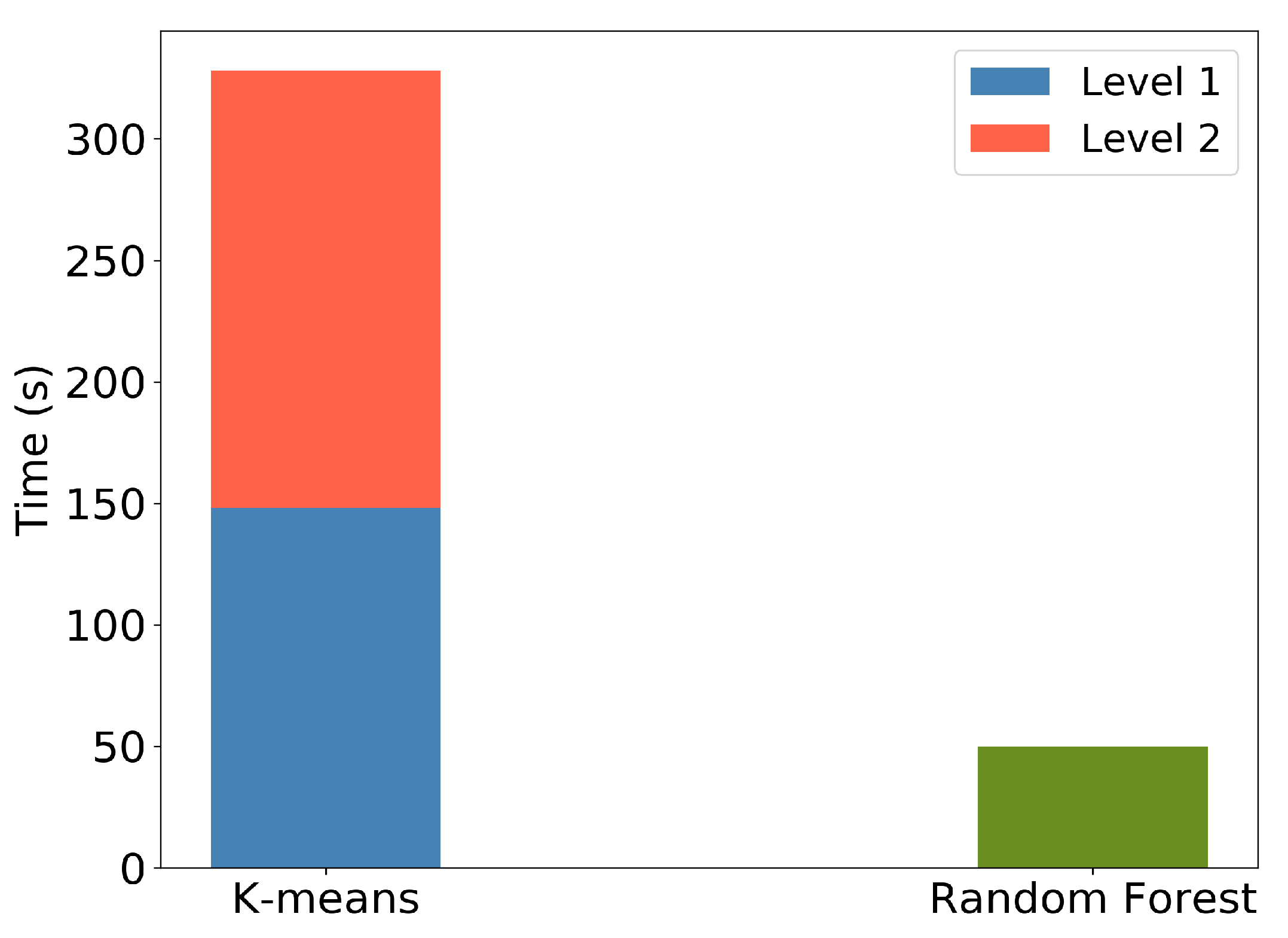
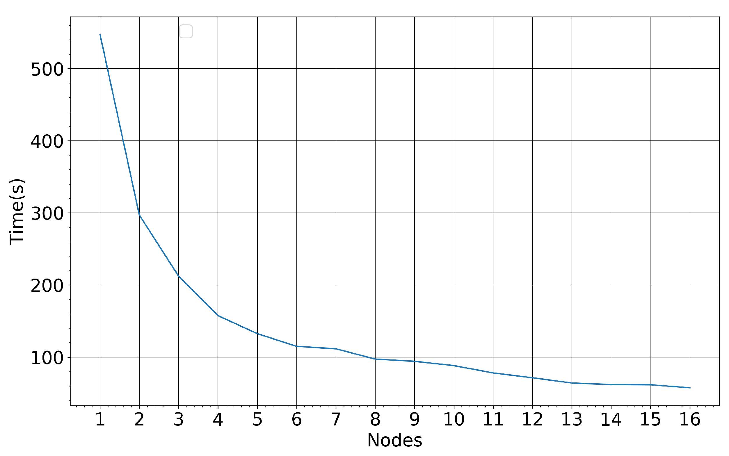
4.2. Model Performance for Varying Training Set Size
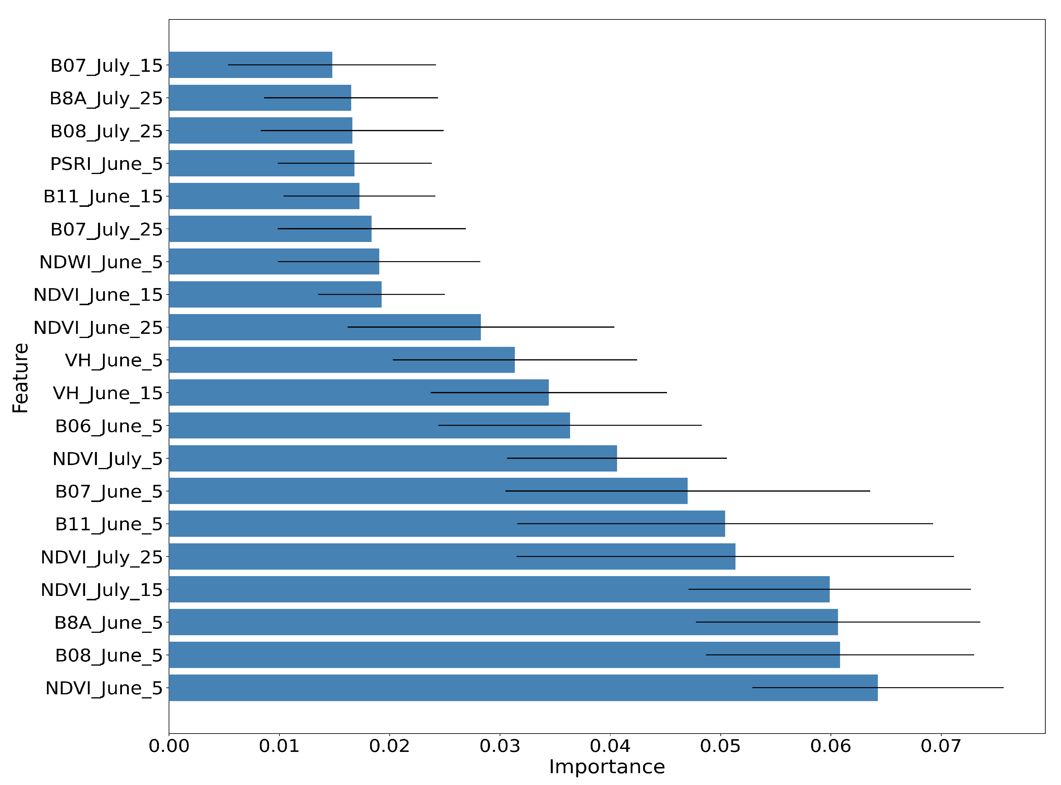
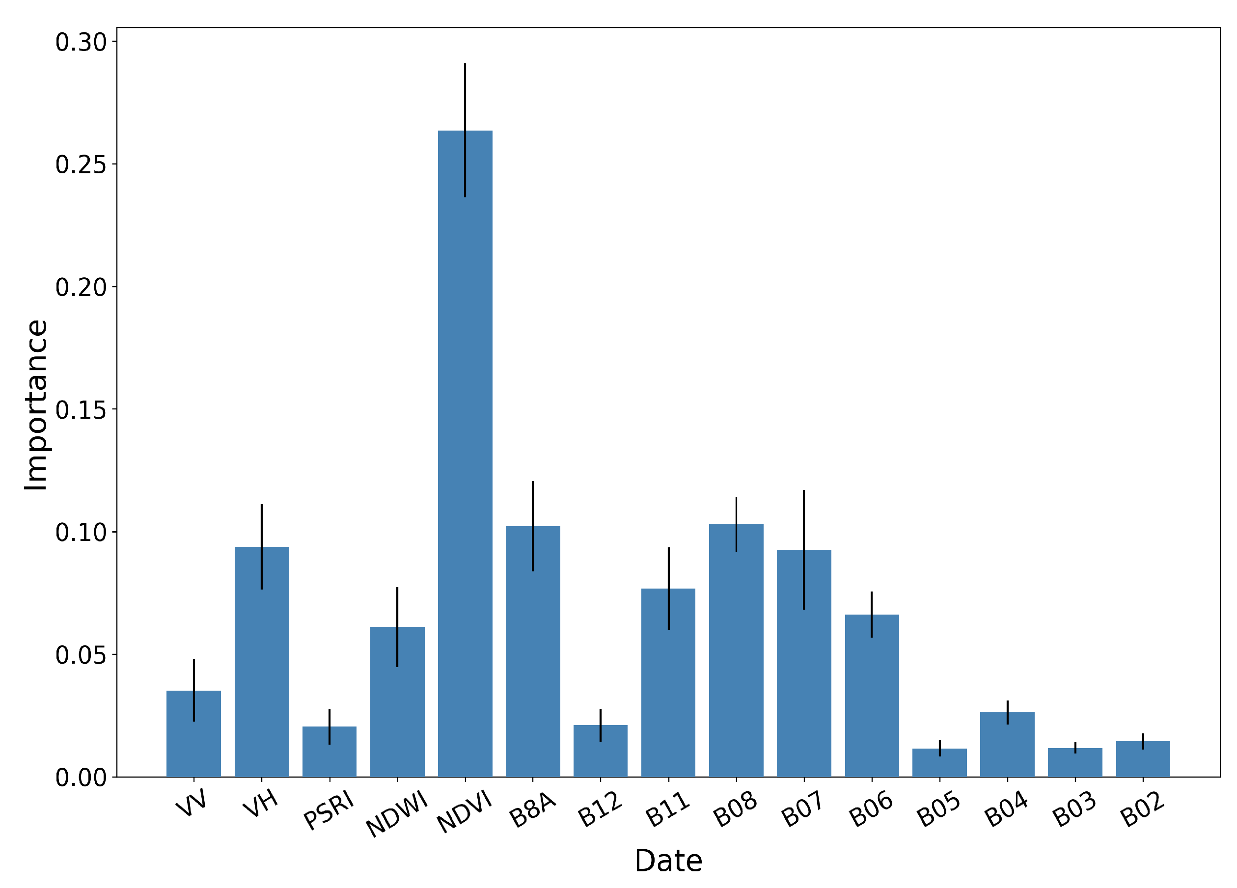
4.3. Feature Importance
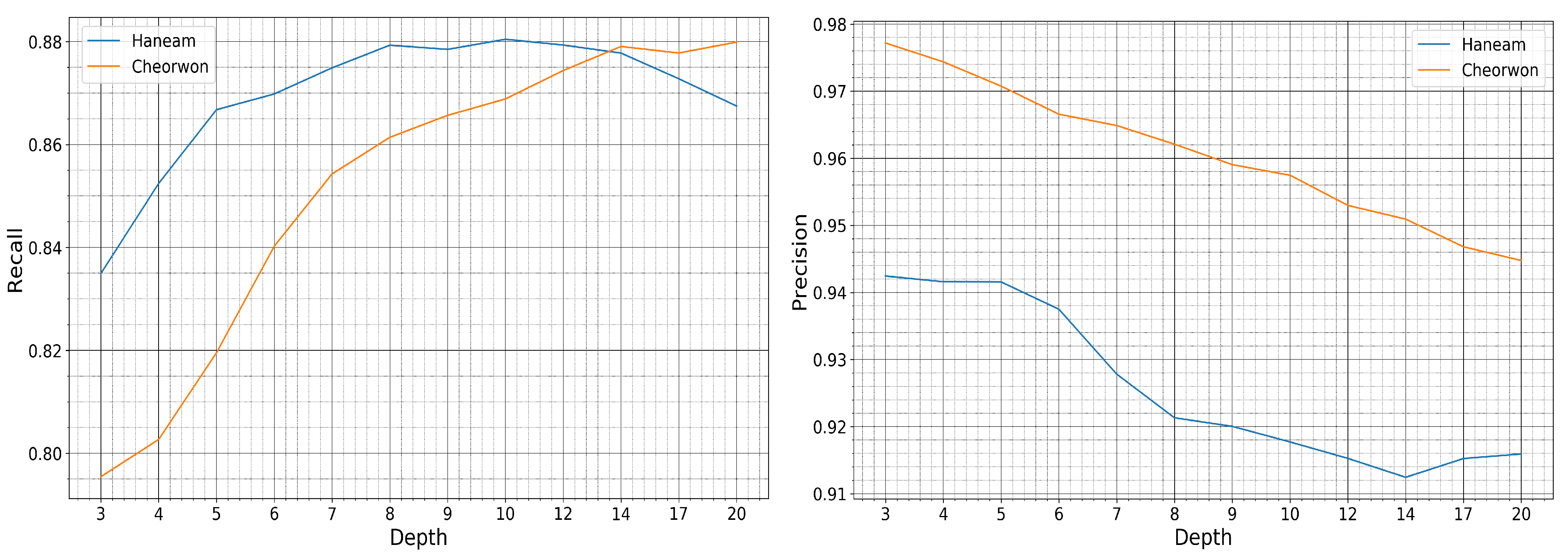
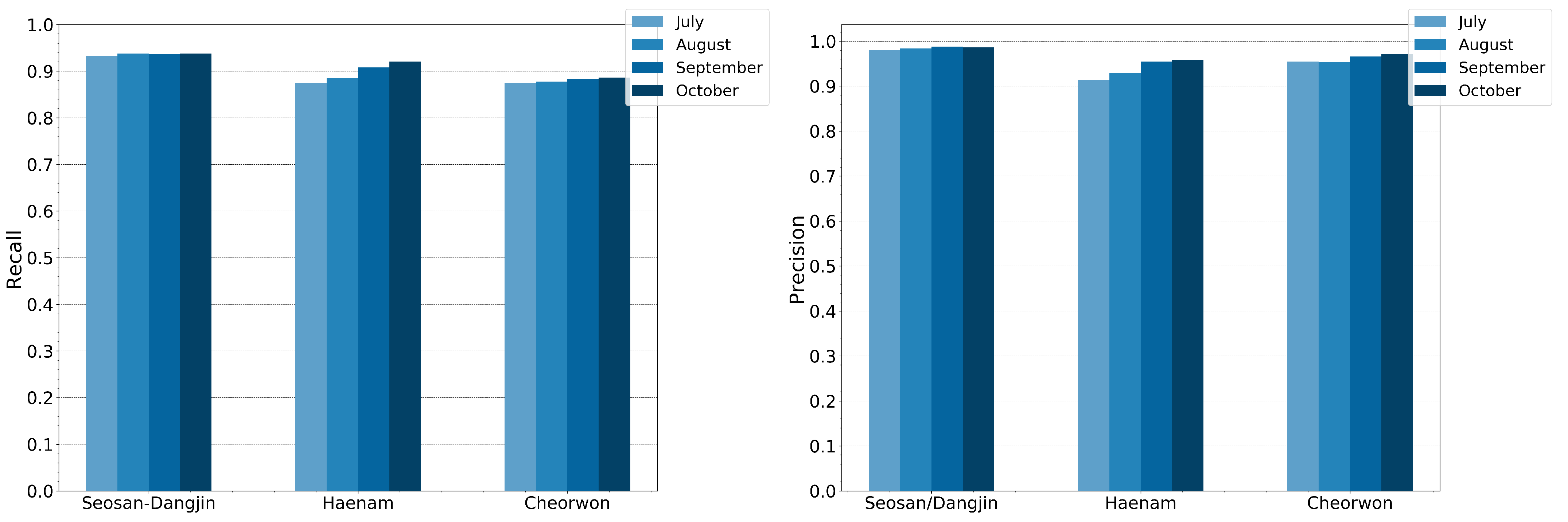
4.4. Accuracy Evolution
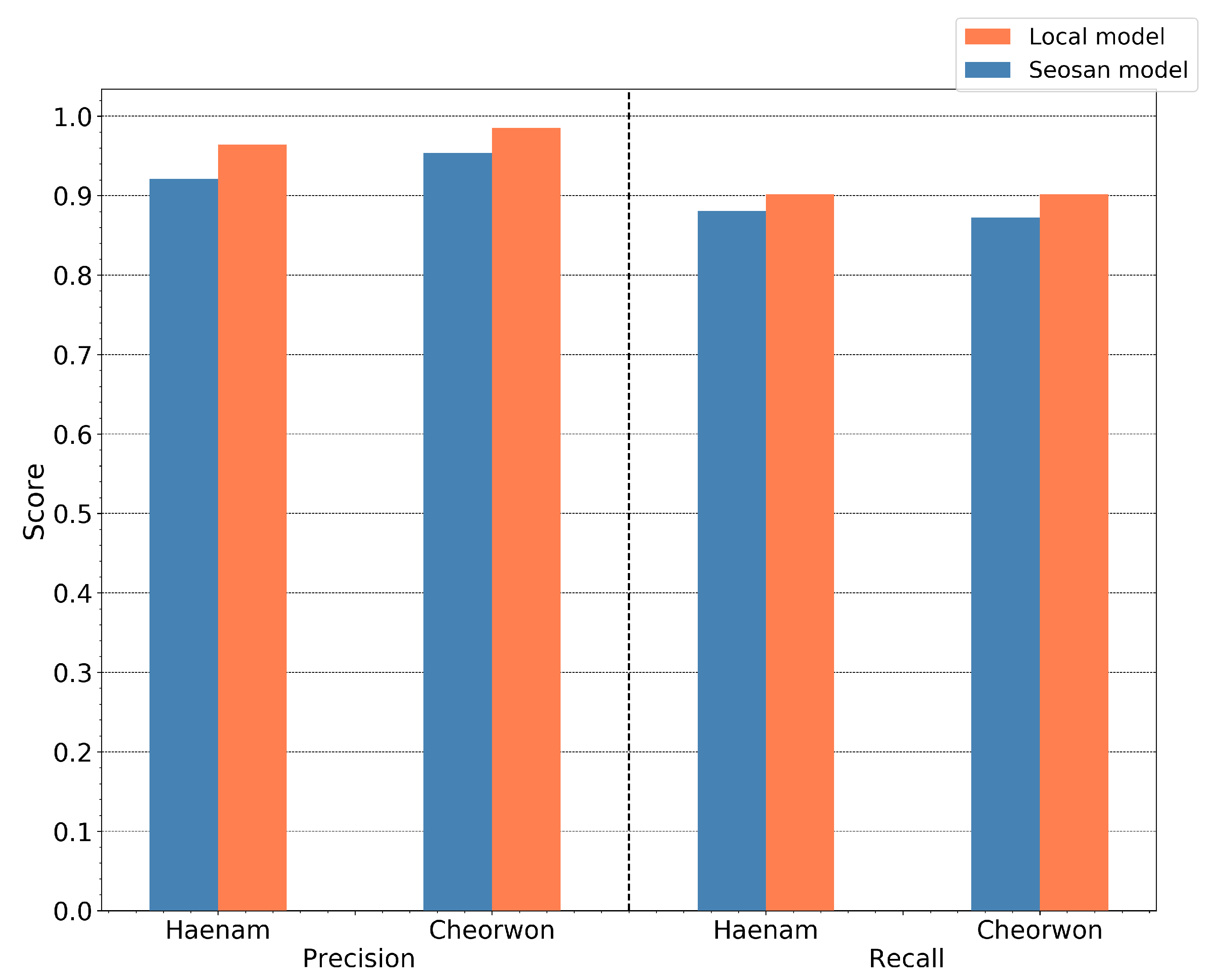
4.5. Model Generalization
5. Discussion
6. Conclusions
Supplementary Materials
Author Contributions
Funding
Data Availability Statement
Acknowledgments
Conflicts of Interest
References
- Fritz, S.; See, L.; You, L.; Justice, C.; Becker-Reshef, I.; Bydekerke, L.; Cumani, R.; Defourny, P.; Erb, K.H.; Foley, J.; et al. The Need for Improved Maps of Global Cropland. Eos Trans. Am. Geophys. Union 2013, 94, 31–32. [Google Scholar] [CrossRef]
- Ban, Y.; Gong, P.; Chandra, G. Global land cover mapping using Earth observation satellite data: Recent progresses and challenges. ISPRS J. Photogramm. Remote Sens. 2015, 1–6. [Google Scholar] [CrossRef] [Green Version]
- Muthayya, S.; Sugimoto, J.D.; Montgomery, S.; Maberly, G.F. An overview of global rice production, supply, trade, and consumption. Ann. N. Y. Acad. Sci. 2014, 1324, 7–14. [Google Scholar] [CrossRef] [PubMed]
- Wang, M.; Wang, J.; Chen, L. Mapping Paddy Rice Using Weakly Supervised Long Short-Term Memory Network with Time Series Sentinel Optical and SAR Images. Agriculture 2020, 10, 483. [Google Scholar] [CrossRef]
- Lee, H.; Bogner, C.; Lee, S.; Koellner, T. Crop selection under price and yield fluctuation: Analysis of agro-economic time series from South Korea. Agric. Syst. 2016, 148, 1–11. [Google Scholar] [CrossRef]
- Rashid, A. Global Information and Early Warning System on Food and Agriculture (GIEWS). Encyclopedia of Life Support Systems (EOLSS). Switzerland. 2009. Available online: https://www.eolss.net/Sample-Chapters/C15/E1-47-14.pdf (accessed on 30 April 2021).
- Becker-Reshef, I.; Justice, C.; Sullivan, M.; Vermote, E.; Tucker, C.; Anyamba, A.; Small, J.; Pak, E.; Masuoka, E.; Schmaltz, J.; et al. Monitoring global croplands with coarse resolution earth observations: The Global Agriculture Monitoring (GLAM) project. Remote Sens. 2010, 2, 1589–1609. [Google Scholar] [CrossRef] [Green Version]
- Rembold, F.; Meroni, M.; Urbano, F.; Csak, G.; Kerdiles, H.; Perez-Hoyos, A.; Lemoine, G.; Leo, O.; Negre, T. ASAP: A new global early warning system to detect anomaly hot spots of agricultural production for food security analysis. Agric. Syst. 2019, 168, 247–257. [Google Scholar] [CrossRef]
- Whitcraft, A.K.; Becker-Reshef, I.; Justice, C.O. A framework for defining spatially explicit earth observation requirements for a global agricultural monitoring initiative (GEOGLAM). Remote Sens. 2015, 7, 1461–1481. [Google Scholar] [CrossRef] [Green Version]
- Xiao, X.; Boles, S.; Frolking, S.; Li, C.; Babu, J.Y.; Salas, W.; Moore, B., III. Mapping paddy rice agriculture in South and Southeast Asia using multi-temporal MODIS images. Remote Sens. Environ. 2006, 100, 95–113. [Google Scholar] [CrossRef]
- Gumma, M.K.; Nelson, A.; Thenkabail, P.S.; Singh, A.N. Mapping rice areas of South Asia using MODIS multitemporal data. J. Appl. Remote Sens. 2011, 5, 053547. [Google Scholar] [CrossRef] [Green Version]
- Pittman, K.; Hansen, M.C.; Becker-Reshef, I.; Potapov, P.V.; Justice, C.O. Estimating Global Cropland Extent with Multi-year MODIS Data. Remote Sens. 2010, 2, 1844–1863. [Google Scholar] [CrossRef] [Green Version]
- Zhang, G.; Xiao, X.; Dong, J.; Kou, W.; Jin, C.; Qin, Y.; Zhou, Y.; Wang, J.; Menarguez, M.A.; Biradar, C. Mapping paddy rice planting areas through time series analysis of MODIS land surface temperature and vegetation index data. ISPRS J. Photogramm. Remote Sens. 2015, 106, 157–171. [Google Scholar] [CrossRef] [Green Version]
- Peng, D.; Huete, A.R.; Huang, J.; Wang, F.; Sun, H. Detection and estimation of mixed paddy rice cropping patterns with MODIS data. Int. J. Appl. Earth Obs. Geoinf. 2011, 13, 13–23. [Google Scholar] [CrossRef]
- Xiao, X.; Boles, S.; Liu, J.; Zhuang, D.; Frolking, S.; Li, C.; Salas, W.; Moore, B., III. Mapping paddy rice agriculture in southern China using multi-temporal MODIS images. Remote Sens. Environ. 2005, 95, 480–492. [Google Scholar] [CrossRef]
- Dong, J.; Xiao, X.; Menarguez, M.A.; Zhang, G.; Qin, Y.; Thau, D.; Biradar, C.; Moore, B., III. Mapping paddy rice planting area in northeastern Asia with Landsat 8 images, phenology-based algorithm and Google Earth Engine. Remote Sens. Environ. 2016, 185, 142–154. [Google Scholar] [CrossRef] [PubMed] [Green Version]
- Kontgis, C.; Schneider, A.; Ozdogan, M. Mapping rice paddy extent and intensification in the Vietnamese Mekong River Delta with dense time stacks of Landsat data. Remote Sens. Environ. 2015, 169, 255–269. [Google Scholar] [CrossRef]
- Qin, Y.; Xiao, X.; Dong, J.; Zhou, Y.; Zhu, Z.; Zhang, G.; Du, G.; Jin, C.; Kou, W.; Wang, J.; et al. Mapping paddy rice planting area in cold temperate climate region through analysis of time series Landsat 8 (OLI), Landsat 7 (ETM+) and MODIS imagery. ISPRS J. Photogramm. Remote Sens. 2015, 105, 220–233. [Google Scholar] [CrossRef] [Green Version]
- Nelson, A.; Setiyono, T.; Rala, A.B.; Quicho, E.D.; Raviz, J.V.; Abonete, P.J.; Maunahan, A.A.; Garcia, C.A.; Bhatti, H.Z.M.; Villano, L.S.; et al. Towards an operational SAR-based rice monitoring system in Asia: Examples from 13 demonstration sites across Asia in the RIICE project. Remote Sens. 2014, 6, 10773–10812. [Google Scholar] [CrossRef] [Green Version]
- Shao, Y.; Fan, X.; Liu, H.; Xiao, J.; Ross, S.; Brisco, B.; Brown, R.; Staples, G. Rice monitoring and production estimation using multitemporal RADARSAT. Remote Sens. Environ. 2001, 76, 310–325. [Google Scholar] [CrossRef]
- Jo, H.W.; Lee, S.; Park, E.; Lim, C.H.; Song, C.; Lee, H.; Ko, Y.; Cha, S.; Yoon, H.; Lee, W.K. Deep Learning Applications on Multitemporal SAR (Sentinel-1) Image Classification Using Confined Labeled Data: The Case of Detecting Rice Paddy in South Korea. IEEE Trans. Geosci. Remote. Sens. 2020, 58, 7589–7601. [Google Scholar] [CrossRef]
- Chebbi, I.; Boulila, W.; Farah, I.R. Big data: Concepts, challenges and applications. In Computational Collective Intelligence; Springer: Berlin/Heidelberg, Germany, 2015; pp. 638–647. [Google Scholar]
- Inglada, J.; Vincent, A.; Arias, M.; Sicre, C. Improved Early Crop Type Identification By Joint Use of High Temporal Resolution SAR And Optical Image Time Series. Remote Sens. 2016, 8, 362. [Google Scholar] [CrossRef] [Green Version]
- Immitzer, M.; Vuolo, F.; Atzberger, C. First Experience with Sentinel-2 Data for Crop and Tree Species Classifications in Central Europe. Remote Sens. 2016, 8, 166. [Google Scholar] [CrossRef]
- Sitokonstantinou, V.; Papoutsis, I.; Kontoes, C.; Arnal, A.; Andrés, A.P.; Zurbano, J.A. Scalable Parcel-Based Crop Identification Scheme Using Sentinel-2 Data Time-Series for the Monitoring of the Common Agricultural Policy. Remote Sens. 2018, 10, 911. [Google Scholar] [CrossRef] [Green Version]
- Rousi, M.; Sitokonstantinou, V.; Meditskos, G.; Papoutsis, I.; Gialampoukidis, I.; Koukos, A.; Karathanassi, V.; Drivas, T.; Vrochidis, S.; Kontoes, C.; et al. Semantically enriched crop type classification and Linked Earth Observation Data to support the Common Agricultural Policy monitoring. IEEE J. Sel. Top. Appl. Earth Obs. Remote. Sens. 2020. [Google Scholar] [CrossRef]
- Tian, H.; Wu, M.; Wang, L.; Niu, Z. Mapping early, middle and late rice extent using sentinel-1A and Landsat-8 data in the poyang lake plain, China. Sensors 2018, 18, 185. [Google Scholar] [CrossRef] [Green Version]
- Torbick, N.; Chowdhury, D.; Salas, W.; Qi, J. Monitoring rice agriculture across myanmar using time series Sentinel–1 assisted by Landsat–8 and PALSAR–2. Remote Sens. 2017, 9, 119. [Google Scholar] [CrossRef] [Green Version]
- Nguyen, D.B.; Gruber, A.; Wagner, W. Mapping rice extent and cropping scheme in the Mekong Delta using Sentinel-1A data. Remote Sens. Lett. 2016, 7, 1209–1218. [Google Scholar] [CrossRef]
- Lee, C.G.; Kim, J.; Shon, J.; Yang, W.H.; Yoon, Y.H.; Choi, K.J.; Kim, K.S. Impacts of Climate Change on Rice Production and Adaptation Method in Korea as Evaluated by Simulation Study. J. Korean Soc. Agric. For. Meteorol. 2012, 14, 207–221. [Google Scholar] [CrossRef]
- Kim, Y.; Shim, K.; Jung, M.; Choi, I.; Kang, K. Classification of agroclimatic zones considering the topography characteristics in South Korea. J. Clim. Chang. Res. 2016, 7, 507–512. [Google Scholar] [CrossRef]
- Chung, J.; Lee, Y.; Jang, W.; Lee, S.; Kim, S. Correlation Analysis between Air Temperature and MODIS Land Surface Temperature and Prediction of Air Temperature Using TensorFlow Long Short-Term Memory for the Period of Occurrence of Cold and Heat Waves. Remote Sens. 2020, 12, 3231. [Google Scholar] [CrossRef]
- Jeong, S.; Ko, J.; Yeom, J. Nationwide Projection of Rice Yield Using a Crop Model Integrated with Geostationary Satellite Imagery: A Case Study in South Korea. Remote Sens. 2018, 10, 1665. [Google Scholar] [CrossRef] [Green Version]
- Park, S.; Im, J.; Park, S.; Yoo, C.; Han, H.; Rhee, J. Classification and Mapping of Paddy Rice by Combining Landsat and SAR Time Series Data. Remote Sens. 2018, 10, 447. [Google Scholar] [CrossRef] [Green Version]
- Xin, F.; Xiao, X.; Zhao, B.; Miyata, A.; Baldocchi, D.; Knox, S.; Kang, M.; Shim, K.; Min, S.; Chen, B.; et al. Modeling gross primary production of paddy rice cropland through analyses of data from CO2 eddy flux tower sites and MODIS images. Remote Sens. Environ. 2017, 190, 42–55. [Google Scholar] [CrossRef] [Green Version]
- Ryu, Y.; Kang, S.; Moon, S.; Kim, J. Evaluation of land surface radiation balance derived from moderate resolution imaging spectroradiometer (MODIS) over complex terrain and heterogeneous landscape on clear sky days. Agric. For. Meteorol. 2008, 148, 1538–1552. [Google Scholar] [CrossRef]
- Yeom, J.; Jeong, S.; Jeong, G.; Ng, C.; Deo, R.; Ko, J. Monitoring paddy productivity in North Korea employing geostationary satellite images integrated with GRAMI–rice model. Sci. Rep. 2018, 8, 1–15. [Google Scholar] [CrossRef] [PubMed] [Green Version]
- Amarsaikhan, D.; Saandar, M.; Ganzorig, M.; Blotevogel, H.; Egshiglen, E.; Gantuyal, R.; Nergui, B.; Enkhjargal, D. Comparison of multisource image fusion methods and land cover classification. Int. J. Remote Sens. 2012, 33, 2532–2550. [Google Scholar] [CrossRef]
- Niu, X.; Ban, Y. Multi-temporal RADARSAT-2 polarimetric SAR data for urban land-cover classification using an object-based support vector machine and a rule-based approach. Int. J. Remote Sens. 2013, 34, 1–26. [Google Scholar] [CrossRef]
- Sheoran, A.; Haack, B. Classification of California agriculture using quad polarization radar data and Landsat Thematic Mapper data. GIScience Remote Sens. 2013, 50, 50–63. [Google Scholar] [CrossRef]
- Xie, L.; Zhang, H.; Wu, F.; Wang, C.; Zhang, B. Capability of Rice Mapping Using Hybrid Polarimetric SAR Data. IEEE J. Sel. Top. Appl. Earth Obs. Remote Sens. 2015, 8, 3812–3822. [Google Scholar] [CrossRef]
- Louis, J.; Debaecker, V.; Pflug, B.; Main-Knorn, M.; Bieniarz, J.; Mueller-Wilm, U.; Cadau, E.; Gascon, F. Sentinel-2 Sen2Cor: L2A processor for users. In Proceedings Living Planet Symposium 2016; Spacebooks Online; Spacebooks Online: Oberpfaffenhofen, Germany, 2016; pp. 1–8. [Google Scholar]
- Muller-Wilm, U.; Louis, J.; Richter, R.; Gascon, F.; Niezette, M. Sentinel-2 level 2A prototype processor: Architecture, algorithms and first results. In Proceedings of the ESA Living Planet Symposium, Edinburgh, UK, 9–13 September 2013; pp. 9–13. [Google Scholar]
- Tucker, C.J. Red and photographic infrared linear combinations for monitoring vegetation. Remote Sens. Environ. 1979, 8, 127–150. [Google Scholar] [CrossRef] [Green Version]
- Gao, B. NDWI—A normalized difference water index for remote sensing of vegetation liquid water from space. Remote Sens. Environ. 1996, 58, 257–266. [Google Scholar] [CrossRef]
- Merzlyak, M.N.; Gitelson, A.A.; Chivkunova, O.B.; Rakitin, V.Y. Non-destructive optical detection of pigment changes during leaf senescence and fruit ripening. Physiol. Plant. 1999, 106, 135–141. [Google Scholar] [CrossRef] [Green Version]
- Sun, R.; Chen, S.; Su, H.; Mi, C.; Jin, N. The Effect of NDVI Time Series Density Derived from Spatiotemporal Fusion of Multisource Remote Sensing Data on Crop Classification Accuracy. ISPRS Int. J. Geo-Inf. 2019, 8, 502. [Google Scholar] [CrossRef] [Green Version]
- Lebourgeois, V.; Dupuy, S.; Vintrou, E.; Ameline, M.; Butler, S.; Bégué, A. A Combined Random Forest and OBIA Classification Scheme for Mapping Smallholder Agriculture at Different Nomenclature Levels Using Multisource Data (Simulated Sentinel-2 Time Series, VHRS and DEM). Remote Sens. 2017, 9, 259. [Google Scholar] [CrossRef] [Green Version]
- Huang, J.; Wang, H.; Dai, Q.; Han, D. Analysis of NDVI Data for Crop Identification and Yield Estimation. IEEE J. Sel. Top. Appl. Earth Obs. Remote Sens. 2014, 7, 4374–4384. [Google Scholar] [CrossRef]
- Inglada, J.; Arias, M.; Tardy, B.; Hagolle, O.; Valero, S.; Morin, D.; Dedieu, G.; Sepulcre, G.; Bontemps, S.; Defourny, P.; et al. Assessment of an Operational System for Crop Type Map Production Using High Temporal and Spatial Resolution Satellite Optical Imagery. Remote Sens. 2015, 7, 12356–12379. [Google Scholar] [CrossRef] [Green Version]
- Hatfield, J.L.; Prueger, J.H. Value of Using Different Vegetative Indices to Quantify Agricultural Crop Characteristics at Different Growth Stages under Varying Management Practices. Remote Sens. 2010, 2, 562–578. [Google Scholar] [CrossRef] [Green Version]
- Sitokonstantinou, V.; Drivas, T.; Koukos, A.; Papoutsis, I.; Kontoes, C. Scalable distributed random forest classification for paddy rice mapping. In Proceedings of the ACRS Conference, Daejeon, Korea, 14–18 October 2019. [Google Scholar]
- Lloyd, S. Least squares quantization in PCM. IEEE Trans. Inf. Theory 1982, 28, 129–137. [Google Scholar] [CrossRef]
- Steinhaus, H. Sur la division des corp materiels en parties. Bull. Acad. Polon. Sci 1956, 1, 801. [Google Scholar]
- Ball, G.; Hall, D. ISODATA, a Novel Method of Data Analysis and Pattern Classification; Technical Report; Stanford Research Inst Menlo Park CA: Menlo Park, CA, USA, 1965. [Google Scholar]
- MacQueen, J. Some methods for classification and analysis of multivariate observations. In Proceedings of the Fifth Berkeley Symposium on Mathematical Statistics and Probability, Oakland, CA, USA, 21 June–18 July 1967; Volume 1, pp. 281–297. [Google Scholar]
- Powers, D. Evaluation: From Precision, Recall and F–Measure to ROC, Informedness, Markedness and Correlation. J. Mach. Learn. Technol. 2011, 2, 37–63. [Google Scholar]
- Lillesand, T.; Kiefer, R.; Chipman, J. Remote Sensing and Image Interpretation; Wiley: New York, NY, USA, 1960; pp. 37–46. [Google Scholar]
- Cohen, J. A Coefficient of Agreement for Nominal Scales. Educ. Psychol. Meas. 1960, 20, 37–46. [Google Scholar] [CrossRef]
- Van Rijsbergen, C. Information Retrieval; Butterworth-Heinemann: London, UK, 1979; p. 208. [Google Scholar]
- Breiman, L. Random forests. Mach. Learn. 2001, 45, 5–32. [Google Scholar] [CrossRef] [Green Version]
- Panda, B.; Herbach, J.S.; Basu, S.; Bayardo, R.J. PLANET: Massively Parallel Learning of Tree Ensembles with MapReduce. In Proceedings of the 35th International Conference on Very Large Data Bases (VLDB-2009), Lyon, France, 24–28 August 2009. [Google Scholar]
- Databricks. Random Forests and Boosting in MLlib. Available online: https://databricks.com/ (accessed on 5 May 2019).


| Seosan/Dangjin | Haenam | Cheorwon | |
|---|---|---|---|
| Mean Elevation (m) | 37 | 45 | 215 |
| Annual Mean Temperature (C) | 11.911.4 | 13.4 | 10.2 |
| Annual Mean Precipitation (mm) | 1285.7/1158.7 | 1325.4 | 1391.2 |
| Annual Mean Humidity (%) | 74.1 | 73.4 | 70.4 |
| Climate zone | Central | Southern | Northern |
| Agro-climatic zone | Western central plain [30]/Zone 2 [31] | South western coastal [30]/Zone 1 [31] | Northern central inland [30]/Zone 4, 5 [31] |
| Rice area 2018 (ha) | 37,728 (sum) | 18,484 | 9429 |
| Rice yield 2018 (tons) | 206,475 (sum) | 89,106 | 52,653 |
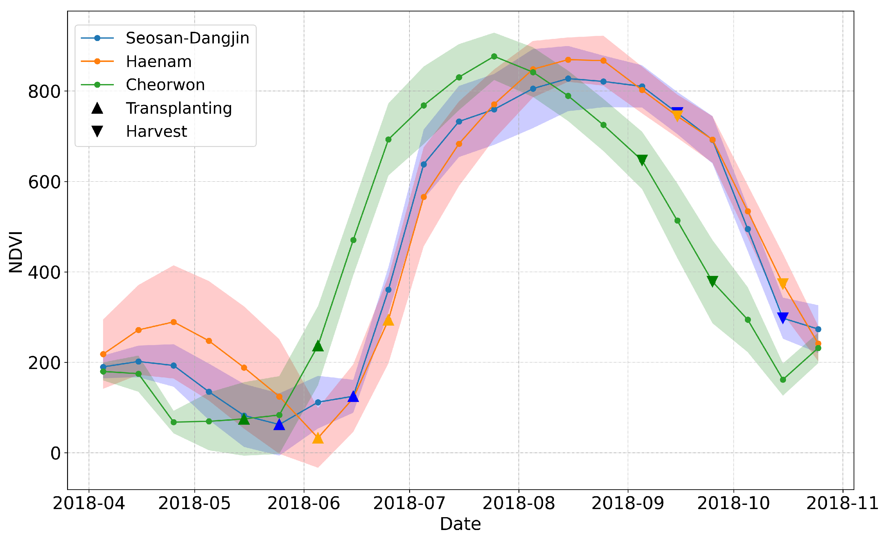
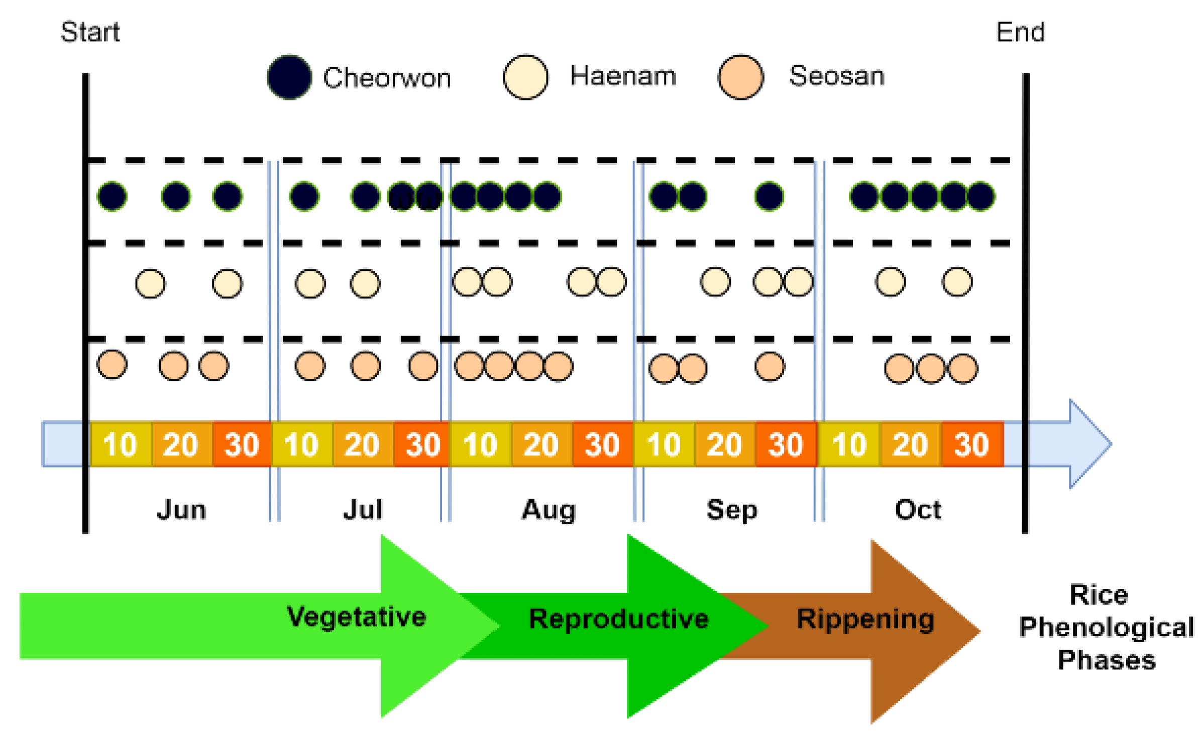
| Rice transplanting | late May—mid June | early—mid June | mid—late May |
| Rice harvesting | early September to mid October | late September to early October | early to mid September |
| Class | Site | Precision | Recall | F1-Score | Clusters |
|---|---|---|---|---|---|
| Rice | Seosan/Dangjin | 97.01% | 91.82% | 94.35% | 7 |
| Haenam | 94.16% | 88.09% | 91.03% | 8 | |
| Cheorwon | 97.63% | 88.59% | 92.89% | 7 | |
| Non Rice | Seosan/Dangjin | 93.91% | 97.81% | 95.82% | 7 |
| Haenam | 96.45% | 98.34% | 97.93% | 8 | |
| Cheorwon | 98.02% | 99.62% | 98.81% | 7 |
| Site | KOSIS Area (ha) | Predicted Area (ha) | Deviation |
|---|---|---|---|
| Seosan & Dangjin | 37,728 | 37,033 | –1.84% |
| Haenam | 18,484 | 17,969 | –2.78% |
| Cheorwon | 9429 | 9854 | +4.50% |
| Model | Type | A | B | C | D | E | F | G | H | I | J | Total |
|---|---|---|---|---|---|---|---|---|---|---|---|---|
| July | Agriculture | 87.47 | 93.16 | 93.04 | 90.67 | 89.14 | 90.10 | 84.56 | 91.71 | 83.33 | 88.10 | 89.13 |
| Urban | 99.60 | 99.97 | 99.99 | 99.66 | 98.43 | 95.80 | 94.03 | 99.65 | 100.00 | 99.84 | 98.70 | |
| Forestry | 100.00 | 100.00 | 100.00 | 99.66 | 99.95 | 99.65 | 99.53 | 99.90 | 100.00 | 100.00 | 99.87 | |
| Water | 100.00 | 100.00 | 99.99 | 99.91 | 100.00 | 90.67 | 100.00 | 100.00 | 100.00 | 100.00 | 99.05 | |
| Sites Acc. | 96.77 | 98.28 | 98.26 | 97.48 | 96.88 | 94.05 | 94.53 | 97.81 | 95.83 | 96.99 | 96.69 | |
| Cohen’s Kappa | 0.80 | 0.80 | 0.86 | 0.86 | 0.91 | 0.84 | 0.78 | 0.93 | 0.84 | 0.89 | 0.87 | |
| October | Agriculture | 87.77 | 93.37 | 93.19 | 90.41 | 89.37 | 90.33 | 84.39 | 91.84 | 82.79 | 89.64 | 89.21 |
| Urban | 99.69 | 99.96 | 100.00 | 99.67 | 98.40 | 95.89 | 94.20 | 99.60 | 100.00 | 99.83 | 98.72 | |
| Forestry | 100.00 | 100.00 | 100.00 | 99.65 | 99.94 | 99.66 | 99.51 | 99.91 | 100.00 | 100.00 | 99.87 | |
| Water | 100.00 | 100.00 | 100.00 | 100.00 | 100.00 | 90.77 | 100.00 | 100.00 | 99.99 | 100.00 | 99.05 | |
| Sites Acc. | 96.87 | 98.33 | 98.30 | 97.43 | 96.92 | 94.16 | 94.53 | 97.15 | 96.12 | 97.37 | 96.65 | |
| Cohen’s Kappa | 0.80 | 0.80 | 0.87 | 0.86 | 0.91 | 0.84 | 0.78 | 0.93 | 0.84 | 0.91 | 0.87 |
| k—Clusters | |||||||||
|---|---|---|---|---|---|---|---|---|---|
| Site Id | Labeled Set Size (Pixels) | 5 | 6 | 7 | 8 | 9 | 10 | 11 | 12 |
| 1 | 8 K | 57.56 | 88.23 | 89.93 | 87.62 | 88.11 | 61.99 | 60.97 | 63.34 |
| 2 | 17 K | 66.01 | 96.15 | 96.86 | 95.59 | 96.2 | 80.14 | 79.69 | 80.85 |
| 3 | 39 K | 95.60 | 96.98 | 96.98 | 96.79 | 96.7 | 87.65 | 87.21 | 87.99 |
| 4 | 51 K | 88.96 | 93.71 | 93.85 | 93.00 | 93.07 | 85.40 | 85.21 | 85.59 |
| 5 | 60 K | 97.94 | 99.62 | 99.56 | 99.55 | 99.56 | 96.57 | 96.5 | 96.67 |
| 6 | 85 K | 93.10 | 95.47 | 95.92 | 94.78 | 95.2 | 84.74 | 84.48 | 85.01 |
| 7 | 260 K | 96.46 | 96.57 | 96.68 | 95.98 | 96.13 | 90.26 | 90.12 | 90.55 |
| 8 | 2.5 M | 90.12 | 95.03 | 95.29 | 94.59 | 94.74 | 87.88 | 87.71 | 88.15 |
Publisher’s Note: MDPI stays neutral with regard to jurisdictional claims in published maps and institutional affiliations. |
© 2021 by the authors. Licensee MDPI, Basel, Switzerland. This article is an open access article distributed under the terms and conditions of the Creative Commons Attribution (CC BY) license (https://creativecommons.org/licenses/by/4.0/).
Share and Cite
Sitokonstantinou, V.; Koukos, A.; Drivas, T.; Kontoes, C.; Papoutsis, I.; Karathanassi, V. A Scalable Machine Learning Pipeline for Paddy Rice Classification Using Multi-Temporal Sentinel Data. Remote Sens. 2021, 13, 1769. https://0-doi-org.brum.beds.ac.uk/10.3390/rs13091769
Sitokonstantinou V, Koukos A, Drivas T, Kontoes C, Papoutsis I, Karathanassi V. A Scalable Machine Learning Pipeline for Paddy Rice Classification Using Multi-Temporal Sentinel Data. Remote Sensing. 2021; 13(9):1769. https://0-doi-org.brum.beds.ac.uk/10.3390/rs13091769
Chicago/Turabian StyleSitokonstantinou, Vasileios, Alkiviadis Koukos, Thanassis Drivas, Charalampos Kontoes, Ioannis Papoutsis, and Vassilia Karathanassi. 2021. "A Scalable Machine Learning Pipeline for Paddy Rice Classification Using Multi-Temporal Sentinel Data" Remote Sensing 13, no. 9: 1769. https://0-doi-org.brum.beds.ac.uk/10.3390/rs13091769